low-cost imu implementation via sensor fusion algorithms

Low-Cost IMU Implementation via Sensor Fusion Algorithms in the

Arduino Environment

A Senior Project

Presented to

the Faculty of the Aerospace Engineering Department

California Polytechnic State University, San Luis Obispo

In Partial Fulfillment

Of the Requirements for the Degree

Aerospace Engineering; Bachelor of Science

By

Brandon McCarron

June 2013

© Brandon McCarron

Low-Cost IMU Implementation via Sensor Fusion

Algorithms in the Arduino Environment

Brandon McCarron1

California Polytechnic State University, San Luis Obispo, California, 93407

A multi-phase experiment was conducted at Cal Poly in San Luis Obispo, CA, to design a

low-cost inertial measurement unit composed of a 3-axis accelerometer and 3-axis gyroscope.

Utilizing the growing microprocessor software environment, a 3-axis accelerometer and 3-

axis gyroscope simulated 6 degrees of freedom orientation sensing through sensor fusion. By

analyzing a simple complimentary filter and a more complex Kalman filter, the outputs of

each sensor were combined and took advantage of the benefits of both sensors to improved

results. Gyroscopic drift was removed in the pitch and roll axes using the Kalman filter for

both static and dynamic scenarios. The addition of computationally lean onboard sensor

fusion algorithms in microcontroller software like the Arduino allows for low-cost hardware

implementations of multiple sensors for use in aerospace applications.

I. Introduction

READING and utilizing sensor data to optimize a control system simultaneously reduces system complexity and

cost of potentially expensive all-in-one solutions. Taking advantage of a sensors benefits and mitigating its

disadvantages involves knowledge of control system operation and the applications purpose. In aerospace

applications, accelerometers and gyroscopes are often coupled into an Inertial Measurement Unit (IMU), which

measures orientation based on a number of sensor inputs, known as Degrees of Freedom (DOF). Inertial Navigation

Systems (INS) for spacecraft and aircraft can cost thousands of dollars due to strict accuracy and drift tolerances as

well as high reliability. With the rising interest in hobbyists and flight enthusiasts, low-cost IMUs have made

significant improvements in accuracy to the point where sensor fusion and filters create a viably stable orientation

sensor. Errors due to gyroscopic drift can be on the order of degs/s for low-cost units and accelerometer jitter can

cause systems instability. However, these errors can be mitigated through sensor fusion, introducing more types of

sensors and using them to correct error from one input to another to reduce propagation error. This experiment

discusses the relationship between an accelerometer and gyroscope to illuminate the significance and effectiveness

of sensor fusion and filtering in practice. A laboratory experiment is proven to be affordable for students and faculty

by using a low-cost Micro-Electro-Mechanical Systems (MEMS) accelerometer and gyroscope with an open-source

single-board Arduino microcontroller. By investigating the capabilities of these devices in conjunction with control

filtering and sensor fusion, a 6 DOF IMU on the Arduino Uno provides considerable orientation accuracy on a

budget and has many educational benefits available as well as future application potential for students and faculty.

II. Background

Combining sensors to improve accuracy and sensor output is a common practice in the aerospace industry.

Accelerometers and gyroscopes are used in INS systems as a baseline to discern orientation with respect to a given

body frame of reference. Gyroscopes sense orientation through angular velocity changes and therefore find

orientation, but they have a tendency to drift over time because they only sense changes and have no fixed frame of

reference. The addition of an accelerometers data allows the bias in a gyroscope to be minimized and better

estimated to reduce propagating error and improve orientation readings. Accelerometers sense changes in direction

with respect to gravity which can orient a gyroscope to a more exact angular displacement. However,

accelerometers are more accurate in static calculations, when the system is closer to its fixed reference point

whereas gyroscopes are better at detecting orientation when the system is already in motion. Accelerometers tend to

1 Undergraduate Student, Aerospace Engineering Department

distort accelerations due to external forces as gravitational forces in motion; which accumulates as noise in the

system and erroneous spikes in resulting outputs. While accelerometers sensors react quickly, accumulated error in

accelerometer jitter and noise are not reliable for INS systems alone. With the addition of the long-term accuracy of

a gyroscope combined with the short-term accuracy of the accelerometer, these sensors can be combined to obtain

more accurate orientation readings by utilizing the benefits of each sensor. A few methods to apply sensor fusion

are available to varying degrees of complexity. A complimentary filter is a simple way to combine sensors, as it is a

linear function of a high pass gyroscope filter and low pass accelerometer filter.1 Noisy accelerometer data with

high frequencies are therefore filtered out in the short-term and smoothed out by smoother gyroscope reading.

While the complimentary filter is computationally simple, it has a tendency to lag behind more involved techniques,

such as the Kalman filter. While there are many variations to the Kalman filter that are more complex and not

typically covered in undergraduate study, a one-dimensional version can be implemented to the IMU to validate the

estimate of the complimentary filter.2 The Kalman filter takes a measured value and finds the future estimate by

varying an averaging factor to optimize converging on the actual signal. The averaging factor is weighed by a

measure of the predicted uncertainty, sometimes called the covariance, to pick a value somewhere between the

predicted and measured value. The recursive functionality of the Kalman filter makes it a very popular sensor

fusion algorithm as it does not take a lot of processing power for a better behaving system.

III. Apparatus and Procedure

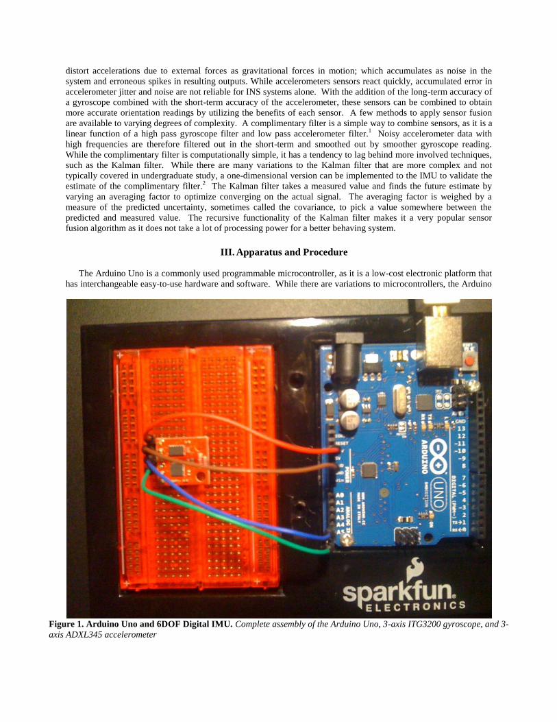
The Arduino Uno is a commonly used programmable microcontroller, as it is a low-cost electronic platform that

has interchangeable easy-to-use hardware and software. While there are variations to microcontrollers, the Arduino

Figure 1. Arduino Uno and 6DOF Digital IMU. Complete assembly of the Arduino Uno, 3-axis ITG3200 gyroscope, and 3-

axis ADXL345 accelerometer

Uno has the necessary Analog In and 3.3V power receptacle for operating the 6 DOF IMU without adding circuitry

or additional hardware. The Arduino Uno, shown in Fig. 1, was attached to the 6 DOF Digital IMU breakout board

by Sparkfun Electronics, shown on the left above the breadboard, which contains a 3-axis accelerometer, ADXL345,

and 3-axis gyroscope, ITG3200. The hardware was connected via A to B USB cabling to a computer containing

Arduino 1.0.5 software for uploading data. Data was processed in the Arduino on-board system and output through

serial connection for analysis and results. Refer to Appendix A for a cost breakdown and purchased parts lists.

The breakout accelerometer and gyroscope

chip are connected to the breadboard by soldering

four break away headers to the appropriate pin

locations. The pins are connected to the 3.3V,

GRND, A4, and A5 on the Arduino. A4 and A5

are designated SDA (data) and SCL (clock) serial

bus interfacings that communicate data between

the two pieces of hardware. As illustrated in

Fig. 2 on the right, cabling from the Arduino to

the IMU is established with male to male jumper

wires attached to the breadboard, which are then

in series with the soldered IMU header pins for

better connectivity.

The Arduino Uno has a 5V power option;

however, that is higher than the allowable range

of the IMU and should not be confused for the

3.3V input as that would likely corrupt collected

data.

IV. Analysis

In order to analyze data provided by the ADXL345 accelerometer and the ITG3200 gyroscope, the raw data

needed to be converted into angular units intelligible for orientation. After reading through the IMU specification

documents for the ADXL345 accelerometer and ITG3200 gyroscope, the below procedure was followed to obtain

pitch and roll orientation information for a complimentary filter and Kalman filter to compare mathematical

complexity to orientation accuracy. This was accomplished in a few steps: reading the IMU ADC with Arduino’s

Wire library, the backbone protocol for the microcontroller, calibrating the sensors data to account for static errors,

and utilizing the accelerometers sense of gravity and rate changes within the gyroscope to find the Euler angles of

the system.

On initialization, samples were taken as an offset criterion for each sensor while the system was

motionless and level to account for static error most likely due to temperature sensitivity, misalignment, or other

unknowns. Solving for the accelerometer output accounting for bias,

(1)

Where is the acceleration, is the offset calibration found on initialization, and is the sensitivity of the

sensor found in the specification sheet for the ADXL345.3 For this model the sensitivity is 256 LSB/g, meaning the

smallest change the sensor can increment positive or negative. Now in output units of -1g to 1g, linear relationships

were found for the x and y axes, or roll φ and pitch θ axes, in order to convert units of g into angular components.

(2)

(3)

Data for the gyroscope was found similarly, except the output for the gyroscope is in LSB per deg/s, a function of

angular velocity with a sensitivity factor of 14.375.4

(4)

3.3V

GND

A4

A5

Figure 2. 6DOF Digital IMU output configuration. Arrows

correspond to the Arduino Uno pin definitions, color-coded

lines match assembly figure.

(5)

Where is the roll rate and is the pitch rate of the gyroscope, is the time step (sampling rate). A

complimentary fusion of sensor data was executed with the following equation for roll, pitch, and yaw:

(6)

Where is the desired angle, is the gyroscope angular velocity output and is related to the time constant,

and the sample rate of the processing code, shown below as:

(7)

The time constant was determined by looking at the cut-off frequency of the gyroscope and accelerometer to define

the boundary in which one sensor “takes over” control of the output the most. Since the gyroscope has a tendency to

drift at a rate of 0.1˚ from inspection, the time constant was set to 0.5 seconds to make sure the system responds

before drift accumulates too much. The time step is the inverse of the sampling frequency, which can be found by

adding a timer in the control loop to see how long calculations take. The larger is, the more the IMU relies on the

gyroscope to estimate the output signal.

Comparatively, the Kalman filter is a much more involved and complex process. As shown in Fig. 3,

there are two main operations between the time and space domain to predict and measure signals.5

Courtesy of "An Introduction to the Kalman filter," the above diagram is a simplified version of the complex filter.

I will not go into detail of each of the units and components yet, as they are well described in the document

reference.6 However, I will simplify and describe the analysis for purposes of this paper. In order to accomplish

sensor fusion, some assumptions were made to simplify the above equations as tabulated in Table 1.

Figure 3. Complete picture of Kalman filter. Diagram displaying the principle action of predicting and correcting

using a Kalman filter.

The error covariance for predicting estimates (from Fig. 3 above in the “Time Update (2)” section) is shown to

be:

(8)

The superscript denotes a prior estimate value, subscript represents time and represents the prior time

value, is the prediction uncertainty, and A is the represents the state space of the model. The state space matrix A

represents for both accelerometer and gyroscope from Eqn. 8, and can be expanded to:

(9)

, represent error covariance, or predicted uncertainty for the accelerometer and gyro and are

initially assumed non-zero constants as it only effects the short-term predictions of the filter, not the long-term

effects.8 is the time step, and Q is the process noise parameter assumed non-zero. Each constant was assumed

initially to be 0.1 arbitrarily in part because I am still learning my way around Kalman filters but also to prove the

prediction process is very smooth even with these initial conditions. Simplification from Fig. 3 and Table 1 give the

following formulas in order from left to right, with some terms in variables specific to this project for clarity:

(10)

Where is the calibration used to offset the static bias prior to sensor fusion. Computational space is precious

for microcontrollers, so Eq. 9 was reduced to an algebraic format:

(11)

The magical Kalman gain, , or the adjusting weight that leads to the estimation of the sensor signals ranging

between the current state and predicted state of the output, is:

(12)

The updated angular estimate at time k for gain is then,

(13)

Finally, updating the error covariance prediction equates to:

Table 1. Defined assumptions for Kalman filtering.

Symbol Definition Value Assumption

Control Input 0 State of system does not change between steps

H Relates current state to measurement 1 Measurement state is equivalent current state

Q Process noise covariance 0.1 Constant chosen to tune filter as in ref. doc.7

R Measurement Noise 5 Driven by accelerometer raw output jitter

(14)

Eqns. 10-14 summarize the step for iterating the Kalman filter through time and space states. It is also important

to note the other three error covariances are similarly defined like Eqn. 12,13, and 14 are the example.

V. Results and Discussion

Prior to calibration, the IMU was recorded to see the effect of drift when the body was not rotated. As Fig. 4

illustrates, gyroscopic drift (at a rate of about .1˚/s) accumulates around each axis of rotation. The gyroscope has no

fixed frame of reference, leaving it to accumulate small errors; whereas the accelerometer remains statically

bounded near zero since the sensor has not viewed changes in the gravitational force applied on it. When the

Kalman filter and Complimentary filter are independently applied to the sensor outputs to create a single output, it is

evident that the two filters are comparable but have a few distinct qualities.

The IMU was also rotated about the pitching y-axis to illustrate the difference between a dynamic accelerometer

and gyroscope before filters are applied. Fig. 5 clearly captures the accelerometer jitter and gyroscopes smooth

trend. The accelerometer approaches the actual angle much quicker than the gyroscope, but without a true measure

of the angle imparted on the IMU, this experiment can only compare and assess by pro and con evaluation of each

gradient.

Also shown in Fig. 5, after gyroscopic drift was allowed to accumulate within the IMU in a stationary position

on a flat surface, a roughly 90˚ rotation was applied about the y-axis. The complimentary filter clearly stays

attached to the gyroscope, indicating the cut-off frequency for this filter should be adjusted (the 100 Hz internal cut-

Figure 4. Static gyroscopic drift. Accumulating error in rotation rate readings within the gyroscope result in

propagating errors if left uncorrected by the accelerometer.

off high pass filter on the gyroscope is not editing out unwanted noise) in order to give more confidence to the

accelerometer. Future experiments should look into phase diagrams to determine the optimal α to tune the cut-off

frequency and reduce system lag when using a Complimentary filter.

Conversely, the Kalman filter does not drift with the gyroscope and follows a smooth trajectory through the

accelerometer noise and returns to zero without any apparent lag behind the accelerometer.

Figure 5. Accumulated drift on complimentary filter requires tuning. The Complimentary high pass filter’s time

constant was set too low and consequently the Complimentary filter did not fringe the accelerometer curve.

After tuning the Complimentary filter’s time constant to a lower value closer to the sample rate, Fig. 6 illustrates a

better curve fit to the accelerometers output angle.

Figure 6. Tuned Complimentary filter. Experimenting trial and error to better compare the Complimentary filter to

the Kalman filter.

Fig. 7 shows how the Filters respond to additional noise due to shaking in the yaw and roll axes during ascent and

descent about the pitch axis. Both filters behave similarly and drive a similar output.

Figure 7. Horizontal shaking of IMU during pitch maneuver. Filter testing for additional error in shaking motion.

Furthermore, Fig. 8 monitors the output of the IMU pitching during very high frequency. Despite vibrations

propagating error in the accelerometer short-term output, both filters compensate remarkably well.

The simplicity of the complimentary filter, a single line of algebra in code, is computationally advantageous for

very lean process environments; however for most microprocessors out to date, the addition of a bit more upfront

legwork to establish a functional Kalman filter has a few more advantages. The complex functions serve to remove

part of the tuning process in place of constants or known qualities about the desired control system. Also, the

absence of drift accumulating in the pitch and roll axes creates a more hands free environment that is applicable to

balancing ground vehicles and helicopters.

VI. Conclusion

The purpose of this experiment was to gain insight into the functionality and purpose of accelerometers,

gyroscopes, and their combination. While many commercial units of IMU’s exist, buying low-cost components and

implementing software is a viable option to not only save money on hardware, but to learn about how systems work

together. With the advancements in microprocessor technology, like the Arduino Uno, computational complexity is

deliverable and consequently gives students or enthusiasts the ability to learn-by-doing getting familiar with both

hardware and software. Future experiments may add additional sensors, such as a 3-axis magnetometer for 9 DOF

to eliminate drift, or create a self-stabilizing camera or robot by implementing a control loop of actuators. Balancing

robots, helicopters, or adding a GPS sensor for an INS system can all be accomplished affordably with the

experience and education of techniques like sensor fusion from a Kalman filter.

Figure 8. Vibration tests noise response on IMU output during pitch maneuver. Vibration filters testing for

additional error in dynamic motion.

VII. References 1URL: http://web.mit.edu/scolton/www/filter.pdf [cited 23 March 2013]

2,5,6,7 Bishop, Gary, "An Introduction to the Kalman filter", University of North Carolina at Chapel Hill

Department of Computer Science, 2001

3URL: https://www.sparkfun.com/datasheets/Sensors/Accelerometer/ADXL345.pdf [cited 04 April 2013]

4URL: https://www.sparkfun.com/datasheets/Sensors/Gyro/PS-ITG-3200-00-01.4.pdf [cited 04 April 2013]

8Madgwick, Sebastian O.H., “An efficient orientation filter for inertial and inertial/magnetic sensor arrays,”

University of Bristol, UK. 2010

Appendices

Appendix A: Cost Breakdown

Appendix B: Arduino Code

#include <Wire.h>

int Gyro_output[3], Accel_output[3];

float dt = 0.02;

float Gyro_cal_x, Gyro_cal_y, Gyro_cal_z, Accel_cal_x, Accel_cal_y, Accel_cal_z;

float Gyro_pitch = 0; //Initialize value

float Accel_pitch = 0; //Initial Estimate

float Predicted_pitch = 0; //Initial Estimate

float Gyro_roll = 0; //Initialize value

float Accel_roll = 0; //Initialize value

float Predicted_roll = 0; //Output of Kalman filter

float Q = 0.1; // Prediction Estimate Initial Guess

float R = 5; // Prediction Estimate Initial Guess

float P00 = 0.1; // Prediction Estimate Initial Guess



float Kk0, Kk1;

float Comp_pitch;

float Comp_roll;

unsigned long timer;

unsigned long time;

void writeTo(byte device, byte toAddress, byte val) {

Wire.beginTransmission(device);

Wire.write(toAddress);

Wire.write(val);

Wire.endTransmission();

}

// Adapted from Arduino.cc/forums for reading in sensor data

void readFrom(byte device, byte fromAddress, int num, byte result[]) {

Wire.beginTransmission(device);

Wire.write(fromAddress);

Wire.endTransmission();

Wire.requestFrom((int)device, num);

int i = 0;

while(Wire.available()) {

result[i] = Wire.read();

i++;

}

}

void getGyroscopeReadings(int Gyro_output[]) {

byte buffer[6];

readFrom(0x68,0x1D,6,buffer);

Gyro_output[0] = (((int)buffer[0]) << 8 ) | buffer[1];



}

void getAccelerometerReadings(int Accel_output[]) {

byte buffer[6];

readFrom(0x53,0x32,6,buffer);

Accel_output[0] = (((int)buffer[1]) << 8 ) | buffer[0];



}

void setup() {

int Gyro_cal_x_sample = 0;

int Gyro_cal_y_sample = 0;

int Gyro_cal_z_sample = 0;

int Accel_cal_x_sample = 0;

int Accel_cal_y_sample = 0;

int Accel_cal_z_sample = 0;

int i;

delay(5);

Wire.begin();

Serial.begin(115200); // Registers set

writeTo(0x53,0x31,0x09); //Set accelerometer to 11bit, +/-4g

writeTo(0x53,0x2D,0x08); //Set accelerometer to measure mode

writeTo(0x68,0x16,0x1A); //Set gyro +/-2000deg/sec and 100Hz Low Pass Filter

writeTo(0x68,0x15,0x09); //Set gyro 100Hz sample rate

Serial.print("time\tGyro_pitch\tAccel_pitch\tComp_pitch\tPredicted_pitch\tGyro_roll\tAccel_roll\tComp_roll\tPre

dicted_roll\ty\tp\tr\n");

delay(100);

for (i = 0; i < 100; i += 1) {

getGyroscopeReadings(Gyro_output);

getAccelerometerReadings(Accel_output);

Gyro_cal_x_sample += Gyro_output[0];

Gyro_cal_y_sample += Gyro_output[1];

Gyro_cal_z_sample += Gyro_output[2];

Accel_cal_x_sample += Accel_output[0];

Accel_cal_y_sample += Accel_output[1];

Accel_cal_z_sample += Accel_output[2];

delay(50);

}

Gyro_cal_x = Gyro_cal_x_sample / 100;

Gyro_cal_y = Gyro_cal_y_sample / 100;

Gyro_cal_z = Gyro_cal_z_sample / 100;

Accel_cal_x = Accel_cal_x_sample / 100;

Accel_cal_y = Accel_cal_y_sample / 100;

Accel_cal_z = (Accel_cal_z_sample / 100) - 256; // Raw Accel output in z-direction is in 256 LSB/g due to gravity

and must be off-set by approximately 256

}

void loop() {

timer = millis();

getGyroscopeReadings(Gyro_output);

getAccelerometerReadings(Accel_output);

Accel_pitch = atan2((Accel_output[1] - Accel_cal_y) / 256, (Accel_output[2] - Accel_cal_z) / 256) * 180 / PI;

Gyro_pitch = Gyro_pitch + ((Gyro_output[0] - Gyro_cal_x) / 14.375) * dt;

//if(Gyro_pitch<180) Gyro_pitch+=360; // Keep within range of 0-180 deg to match Accelerometer output

//if(Gyro_pitch>=180) Gyro_pitch-=360;

Comp_pitch = Gyro_pitch;

Predicted_pitch = Predicted_pitch + ((Gyro_output[0] - Gyro_cal_x) / 14.375) * dt; // Time Update step 1

Accel_roll = atan2((Accel_output[0] - Accel_cal_x) / 256, (Accel_output[2] - Accel_cal_z) / 256) * 180 / PI;

Gyro_roll = Gyro_roll - ((Gyro_output[1] - Gyro_cal_y) / 14.375) * dt;

//if(Gyro_roll<180) Gyro_roll+=360; // Keep within range of 0-180 deg

//if(Gyro_roll>=180) Gyro_roll-=360;

Comp_roll = Gyro_roll;

Predicted_roll = Predicted_roll - ((Gyro_output[1] - Gyro_cal_y) / 14.375) * dt; // Time Update step 1

P00 += dt * (2 * P01 + dt * P11); // Projected error covariance terms from derivation result: Time Update step 2

P01 += dt * P11; // Projected error covariance terms from derivation result: Time Update step 2

P00 += dt * Q; // Projected error covariance terms from derivation result: Time Update step 2

P11 += dt * Q; // Projected error covariance terms from derivation result: Time Update step 2

Kk0 = P00 / (P00 + R); // Measurement Update step 1

Kk1 = P01 / (P01 + R); // Measurement Update step 1

Predicted_pitch += (Accel_pitch - Predicted_pitch) * Kk0; // Measurement Update step 2

Predicted_roll += (Accel_roll - Predicted_roll) * Kk0; // Measurement Update step 2

P00 *= (1 - Kk0); // Measurement Update step 3

P01 *= (1 - Kk1); // Measurement Update step 3

P11 -= Kk1 * P01; // Measurement Update step 3

float alpha = 0.98;

Comp_pitch = alpha*(Comp_pitch+Comp_pitch*dt) + (1.0 - alpha)*Accel_pitch; // Complimentary filter

Comp_roll = alpha*(Comp_roll+Comp_roll*dt) + (1.0 - alpha)*Accel_roll; // Complimentary filter

float angle_z = Gyro_output[2];

time=millis();

Serial.print(time);

Serial.print("\t");

Serial.print(Gyro_pitch);

Serial.print("\t");

Serial.print(Accel_pitch);

Serial.print("\t");

Serial.print(Comp_pitch);

Serial.print("\t");

Serial.print(Predicted_pitch);

Serial.print("\t");

Serial.print(Gyro_roll);

Serial.print("\t");

Serial.print(Accel_roll);

Serial.print("\t");

Serial.print(Comp_roll);

Serial.print("\t");

Serial.print(Predicted_roll);

Serial.print("\n");

timer = millis() - timer;

timer = (dt * 1000) - timer;

delay(timer);

}

low-cost imu implementation via sensor fusion algorithms

Documents