UAV manuscript No.(will be inserted by the editor)

Fusion of IMU and Vision for Absolute Scale Estimationin Monocular SLAM

Gabriel Nutzi · Stephan Weiss

Davide Scaramuzza and Roland Siegwart

Received: date / Accepted: date

Abstract The fusion of inertial and visual data is widely used to improve an object’s

pose estimation. However, this type of fusion is rarely used to estimate further un-

knowns in the visual framework. In this paper we present and compare two different

approaches to estimate the unknown scale parameter in a monocular SLAM frame-

work. Directly linked to the scale is the estimation of the object’s absolute velocity

and position in 3D. The first approach is a spline fitting task adapted from Jung and

Taylor and the second is an extended Kalman filter. Both methods have been simu-

lated offline on arbitrary camera paths to analyze their behavior and the quality of the

resulting scale estimation. We then embedded an online multi rate extended Kalman

filter in the Parallel Tracking and Mapping (PTAM) algorithm of Klein and Murray

together with an inertial sensor. In this inertial / monocular SLAM framework, we

show a real time, robust and fast converging scale estimation. Our approach does not

depend on known patterns in the vision part nor a complex temporal synchronization

between the visual and inertial sensor.

The research leading to these results has received funding from the European Community’sSeventh Framework Programme (FP7/2007-2013) under grant agreement n. 231855 (sFly).Gabriel Nutzi is currently a Master student at the ETH Zurich. Stephan Weiss is currentlyPhD student at the ETH Zurich. Davide Scaramuzza is currently senior researcher and teamleader at the ETH Zurich. Roland Siegwart is full professor at the ETH Zurich and head ofthe Autonomous Systems Lab.

G. Nutzi · S. Weiss · D. Scaramuzza · R. SiegwartETH Autonomous Systems Laboratory, 8092, Zurich, Switzerland, www.asl.ethz.chE-mail: nuetzi@student.ethz.ch, stephan.weiss@mavt.ethz.ch, davide.scaramuzza@ieee.org,rsiegwart@ethz.ch

2

1 Introduction

Online pose estimation with sensors on board is important for autonomous robots. We

use an Inertial Measurement Unit (IMU), which is able to measure the 3D acceleration

and rotation of a moving object and a fisheye camera. With each sensor it is possible

to obtain the actual position of the moving vehicle. An integration of the acceleration

measurements over time from the IMU yields a position in meters whereas an applied

SLAM (Simultaneous Localization and Mapping) algorithm on the vision data provides

a position with unknown scale factor λ. By using two cameras, which is not the case

in this study, the scale problem would be solved. However, for example due to weight

restrictions, often only one single camera can be applied. The estimate of the scale

factor is essential to fuse the measurements of both camera and IMU. This fusion leads

to a drift free estimation of the vehicles absolute position and velocity. Both are crucial

parameters for efficient control.

We present two different methods for the scale estimation. The first is an online

spline fitting approach adapted from Jung and Taylor. [1]. The second is a multi rate

Extended Kalman Filter (EKF).

The essence of this study, besides the scale estimation, was also to have a completely

different approach at hand, the spline fitting, which we then can compare to the so

often used EKF. Both approaches have been simulated in Matlab and compared to each

other. The EKF has then been implemented online, because of its better performance.

For the implementation, we modified the source code in the PTAM algorithm of Klein

and Murray [2]. and included some additional parallel tasks which allowed us to filter

both data with a relatively high sample rate. The novelty in this paper is the possibility

to estimate the absolute scale in real time only with the help of a single camera and

a 3D accelerometer. This simple, yet effective method is applicable (on board) on any

vehicle featuring these two devices. Yielding also the absolute position and velocity of

the vehicle the proposed algorithm is directly applicable for control.

This paper is organized as follows: In Section II we discuss the related work. Section

III gives an overview of hardware and inputs used for the algorithms. In section IV

and V the two approaches are outlined and the results are provided for each of them.

They are then discussed in the last section.

2 Related Work

Fusion of vision and IMU data can be classified into Correction, Colligation and Fu-

sion. Whereas the first uses information from one sensor to correct or verify another,

the second category merges different parts of the sensors. For example, Nygards [3]

integrated visual information with GPS to correct the inertial system. Labarosse [4]

suggested using inertial data to verify the results from visual estimation. Zuffery &

Floreano [5] developed a flying robot equipped only with a low resolution visual sen-

sor and a MEMS rate gyro. They introduced gyro data into the absolute optical flow

calculations of two cameras.

EKFs are widely used on the third category. In this paper we focus on the scale

problem which arises due to the combination of monocular vision and inertial data.

Unfortunately, most studies do not consider the scale ambiguity. For example Huster

[6] implemented an EKF to estimate a relative position of an autonomous underwater

vehicle, but the scale has not been included in the state vector. Arnesto et al. [7] fused

3

orientation and position both from camera and inertial sensors in a multi rate EKF for

a 6D tracking task. Stereo vision is used to solve the scale ambiguity directly. Stereo

vision was further used in [7,8,9,10]. Like in [9], huge dimensional states render real

time implementations difficult. Stratmann and Solda [11] used a KF to fuse gyro data

with optical flow calculations. Because no translation was recovered, no scale factor

had to be estimated. Also the authors of [12] and [13] only included orientation. In

[14] they used a single camera to track lane boundaries on a street for autonomous

driving. The authors did not provide information about the scale.Also in Eino et al.

[15], where inertial data from an IMU is fused with the velocity estimation from a vision

algorithm, no details about the scale problem are reported. Ribo et al. [16] proposed

an EKF to fuse vision and inertial data to estimate the 6DoF attitude. There and in

[17,10,18,19] the authors use a priori knowledge to overcome the scale problem. Aid of

an unscented Kalman filter, Kelly estimated the 6 degrees of freedom (DoF) between

a camera and an IMU on a rigid body [20]. In his most recent work he did not use a

known target but uses SLAM and estimates thus also the absolute scale in the offline

estimation as the algorithm is too slow for real time implementation. In this study

we present an online multi rate EKF which provides an accurate estimate of the scale

factor λ in a converging time as fast as 15 seconds. The filter can be implemented

online on any vehicle featuring a camera and a 3D accelerometer. The novelty of our

proposed method does not lie in the sensor fusion as such, but more on its real-time

implementation with the focus to apply it on an embedded platform, thanks to small

matrices in the multi rate EKF. Our approach does neither rely on a complex temporal

calibration of the sensors.

3 Setup & Inputs

For the vision input we used a USB uEye UI-122xLE camera from IDS with a fish-eye

lens. The camera has a resolution of 752 × 480 and a frame rate up to 87 fps. It’s high

dynamic range and global shutter minimized motion blur.

For the inertial inputs, we used the solid state vertical gyro VG400CC-200 from

Crossbow with up to 75Hz, which includes a tri-axial accelerometer and a tri-axial

gyroscope. It has an input range of ± 10 g with a resolution < 1.25 mg. Internally, a

Kalman filter is run which already corrects for the bias and misalignment. The IMU

output is the rotation yaw, pitch and roll and the 3D acceleration ax, ay, az in its

coordinate system C.

The uEye camera was mounted underneath the Crossbow IMU which is shown in

Fig. 1(a). The calibration to obtain the rotation matrix Rca was calculated with the

InerVis IMU CAM calibration toolbox in Matlab [21], see Fig. 1(b). The subscript

’ca’ denotes the rotation from the acceleration frame ’a’ to the camera frame ’c’. In

Fig. 1(b), there are 3 relevant reference frames, W, the fixed world frame, the camera

reference frame C and the IMU frame A which are mounted together.

4

(a) (b)

Fig. 1 a) The Camera/IMU setup. b) Schematics of the reference frames. The subscripts’wc’ denote the rotation from the camera frame C to the world frame W and vice versa. Theacceleration a is measured in the IMU frame and is then resolved in the world frame wherewe subtract the gravitiy vector g.

4 Spline Fitting

4.1 Overview

Jung and Taylor considered the problem of estimating the trajectory of a moving cam-

era by combining the measurements obtained from an IMU with the results obtained

from a structure from motion (SFM) algorithm. They proposed an offline spline fitting

method, where they fit a second order spline into a set of several keyframes obtained

by the SFM algorithm with monocular vision. We used this approach because of the

good results reported by the authors. We modified this spline fitting so that we can

implement it for an online scale estimation. Fig. 2 shows this concept. The black line

belongs to the ground truth path of the Camera/IMU. The blue points are the camera

poses obtained from the visual SLAM algorithm. We assumed noise with a standard

deviation of σv varying from 0.01m/λ to 0.05m/λ, which is close to reality for the

chosen SLAM algorithm. For this visualisation we assume a scale factor λ = 1. We

divide our time line into sections with a fixed duration of Ts = 0.5 to 1.5 seconds.

For each section, three to five second order splines are fitted (green dashed line). The

red curve shows the integrated IMU over the time Ts which is flawed by its drift. The

spline fitting is done continuously when a new section is finished. This introduced time

delay of 0.5 to 1.5 seconds. Note that this can be critical if used in control, albeit the

scale is not prone to sudden changes. By introducing a weighting into the least square

optimization, it is possible to rely more on the acceleration measurements when the

quality of the vision tracking deteriorates as shown in Fig. 2 ’bad tracking’. For each

section we estimate one scale factor λn, which is then averaged over time.

For the simulation in Matlab on arbitrary camera paths, we simplified the following

aspects compared to the original version from Jung and Taylor:

– We assumed that the acceleration of the CAM/IMU is already given in the world

frame. Therefore the subtraction of the gravitation vector g is not necessary.

– The keyframe position are now soft constraints, meaning that a least square is done

between the acceleration measurements and the keyframe points. This differs from

Jung and Taylor, where the keyframes are hard constraints for the fitted spline

curve. This allows more noise and even short periods of wrong tracking in the

visual part.

5

Fig. 2 Concept for the online spline fitting, only x(t) is visualized. In each section Ts we fit 3 -5 second order splines (green dashed line) into the blue points, which are the position withoutscale from the SLAM algorithm. The red line shows the position obtained from integration ofthe acceleration data over time. Each section has its own scale λ.

4.2 Least Square Optimisation

We obtain the following equations for the least square in one section Ts:

The second order spline yields,

min3 to 5X

i=1

˛

˛

˛

˛

˛

˛

˛

˛

˛

˛

˛

˛

0

@

axi + bx

i τj + cxi τ2

j − λxj

ayi + by

i τj + cyi τ2

j − λyj

azi + bz

i τj + czi τ2

j − λzj

1

A

˛

˛

˛

˛

˛

˛

˛

˛

˛

˛

˛

˛

2

(1)

Where [ai, bi, ci] for each direction [x, y, z] and λ are the unknown parameters. The

subscript ’i’ denotes the spline number running from 3 up to 5. τj = (tj − iTs)/Ts and

[xj , yj , zj ] are the positions from the SLAM algorithm spaced over one section (blue

points in Fig. 2).

The continuity constraints at the boundaries of the splines in each section are,

0

@

axi+1

ayi+1

azi+1

1

A =

0

@

axi + bx

i + cxi

ayi + by

i + cyi

azi + bz

i + czi

1

A (2)

0

@

bxi+1

byi+1

bzi+1

1

A =

0

@

bxi + 2cx

i

byi + 2cy

i

bzi + 2cz

i

1

A (3)

The acceleration from spline yields:

aw =

0

@

x

y

z

1

A =2

T 2s

0

@

cxi

cyi

czi

1

A (4)

min

mX

k=1

∥aw(tk) − aw(tk)∥2 (5)

Where the subscript ’w’ denotes the acceleration resolved in the world frame W and

a are the noisy acceleration measurements from the IMU.

6

With equation 1 and 5 we can form a least square problem in the form Az = b

with constraints Cz = 0 from 2,3. The analytical solution to this problem can be found

with Lagrange multipliers. We solved this in Matlab with the function linsq, which

provides linear constraints in a least square problem.

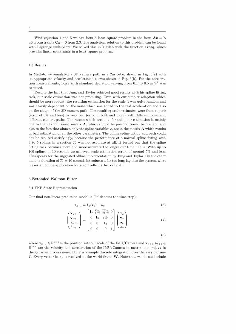
4.3 Results

In Matlab, we simulated a 3D camera path in a 2m cube, shown in Fig. 3(a) with

its appropriate velocity and acceleration curves shown in Fig. 3(b). For the accelera-

tion measurements, noise with standard deviation varying from 0.1 to 0.5 m/s2 was

assumed.

Despite the fact that Jung and Taylor achieved good results with his spline fitting

task, our scale estimation was not promising. Even with our simpler adaption which

should be more robust, the resulting estimation for the scale λ was quite random and

was heavily dependent on the noise which was added to the real acceleration and also

on the shape of the 3D camera path. The resulting scale estimates were from superb

(error of 5% and less) to very bad (error of 50% and more) with different noise and

different camera paths. The reason which accounts for this poor estimation is mainly

due to the ill conditioned matrix A, which should be preconditioned beforehand and

also to the fact that almost only the spline variables ci are in the matrix A which results

in bad estimation of all the other parameters. The online spline fitting approach could

not be realized satisfyingly, because the performance of a normal spline fitting with

3 to 5 splines in a section Ts was not accurate at all. It turned out that the spline

fitting task becomes more and more accurate the longer our time line is. With up to

100 splines in 10 seconds we achieved scale estimation errors of around 5% and less.

This speaks for the suggested offline implementation by Jung and Taylor. On the other

hand, a duration of Ts = 10 seconds introduces a far too long lag into the system, what

makes an online application for a controller rather critical.

5 Extended Kalman Filter

5.1 EKF State Representation

Our final non-linear prediction model is (’k’ denotes the time step),

zk+1 = fk(zk) + νk (6)

0

B

B

@

xk+1

vk+1

ak+1

λk+1

1

C

C

A

=

2

6

6

6

6

4

I3TλI3

T2

2λI3 0

0 I3 T I3 0

0 0 I3 0

0 0 0 1

3

7

7

7

7

5

0

B

B

@

xk

vk

ak

λk

1

C

C

A

(7)

(8)

where xk+1 ∈ R3×1 is the position without scale of the IMU/Camera and vk+1,ak+1 ∈R3×1 are the velocity and acceleration of the IMU/Camera in metric unit [m]. νk is

the gaussian process noise. Eq. 7 is a simple discrete integration over the varying time

T . Every vector in zk is resolved in the world frame W. Note that we do not include

7

−1

0

1

2

3

0

0.5

1

1.5

20

0.2

0.4

0.6

0.8

1

1.2

1.4

[m][m]

[m]

(a)

5 10 15 20 25 30 35 40 45 50t [s]

ax(t)ay(t)az(t)

5 10 15 20 25 30 35 40 45 50t [s]

vx(t)vy(t)vz(t)

5 10 15 20 25 30 35 40 45 50t [s]

ax(t)+ NOISEay(t)+NOISEaz(t)+NOISE

(b)

Fig. 3 Simulated path in its spacial and temporal representation: a) The simulated 3D camerapath in Matlab. b) The simulated velocity, acceleration and the acceleration with added noisefrom the 3D spline in Matlab.

8

the orientation information in the model nor use it as a measurement in order to keep

the algorithm simple and fast. On each acceleration measurement we do the conversion

from the inertial to the world frame by using a zero order hold (ZOH) of the unfiltered

attitude measurement returned by the visual SLAM framework. As we work in a middle

size environment with enough loops we assume negligible drift in the SLAM map and

assume thus highly accurate attitude estimation from the visual SLAM framework.

The model in its linearised form yields,

Fk =

2

6

6

6

6

4

I3TλI3

T2

2λI3 − T

λ2 I3 − T2

2λ2 I3

0 I3 T I3 0

0 0 I3 0

0 0 0 1

3

7

7

7

7

5

(9)

To implement the fusion we consider the measurements in different observation

vectors. For a multirate filter, as it is in our case, the literature suggests two solutions.

One would be using a (higher order) hold to synchronize the different measurements.

Another is to weight the uncertainty of the measurement according to its temporal

occurrence. We used the simplification in [12]. We claim no certainty at all if no mea-

surement is available (i.e. the measurement noise variance is infinite). Thus the update

equations simplify to equations (12)-(14) if vision data arrive or to (15)-(17) if IMU

data arrive. A more complex weighting function (i.e. exponential decay in time) could

also be applied, however, at the cost of speed.

The measurement updates for the vision and the IMU yields (’V’ and ’I’ denotes

Vision and IMU)

yV,k = HV,kzk =ˆ

I3 03 03 0˜

zk (10)

yI,k = HI,kzk =ˆ

03 03 I3 0˜

zk (11)

The innovation for the vision part is,

KV,k = P−k H⊤

V,k(HV,kP−k H⊤

V,k + RV )−1 (12)

zk = zk + KV,k(xSLAM − HV,kzk) (13)

Pk = (I − KV,kHV,k)P−k (14)

The innovation for the IMU part is,

KI,k = P−k H⊤

I,k(HI,kP−k H⊤

I,k + RI)−1 (15)

zk = zk + KI,k(aIMU − HI,kzk) (16)

Pk = (I − KI,kHI,k)P−k (17)

The two matrices RI ,RV are the noise covariance matrices for the vision and IMU

measurement inputs xSLAM ,aIMU which are resolved in the world frame W. The

vector xSLAM is the position without scale obtained from the vision algorithm (SLAM).

The IMU measurement aIMU needs special attention, because significant errors arise

in the conversion from the raw IMU output. According to Fig. 1(b), the acceleration

in the world frame is given by,

wa =RwcRca(aa − b) − wg (18)

9

where aa is the acceleration output from the Crossbow IMU in its coordinate frame A.

b is the static offset of the IMU. The rotation matrix Rwc is provided by the SLAM

algorithm. This rotation is much more accurate than the rotation solely from the IMU

which is integrated over time and suffers from drift. The accuracy of Rwc depends

on the initialization of the map by the SLAM algorithm. With good initialization the

error of the angles are around ±1-2A◦. This error is due to the fact that we did not

adapt the camera model in the SLAM algorithm of Klein and Murray, which is still

perspective and not for fisheye lenses. Another issue which causes significant errors

in the acceleration measurement ca is the fact that our accelerations induced by the

camera motion are small compared to the gravitational field. The subtraction of the

gravitation vector wg then introduces a dynamical bias in ca when the camera rotation

is inaccurate.

5.2 Results with Simulated and Real Data

We have simulated the proposed Kalman filter offline with our 3D path generator (see

spline fitting) and also on real measurement sets. For each measurement set we recorded

the two measurement inputs for the Kalman filter, the vision non-scaled position from

Klein and Murray’s SLAM algorithm and the acceleration from the Crossbow IMU.

For the measurement sets and for the path generator we used the Kalman filter in eq. 7

but with three different setups. The first is the same as in eq. 7. In the second we only

use the Z-axis, meaning that the new state yields [xz,vz,az, λ] and in the third we

use only the X and Y-axis. Fig. 5 shows the scale estimation λ(t) for the simulated 3D

path on the left and for the measurement set on the right. Always the same path and

measurement set was used. To make the measurements of the simulated 3D path close

to the real data, we chose the same standard deviations for the acceleration noise of the

simulated data as measured on the real data (σSLAM = 0.01 (with a λ = 1 → 0.01 m),

σIMU = 0.2 m/s2) The initial velocity and acceleration for the state vector were set to

zero. The initial scale λ was set to the worst case, where the initial value would have an

error of 50 %, which does not normally happen. A simple integration over time of the

acceleration gives an initial guess for the scale with an error in a range of 5-20 %. After

25 seconds we also lower the variance of λ in the state space noise covariance matrix

Q. This produces less overshoot and faster convergence. The two different correction

updates, eq. 15,12 are performed as soon as the measurements arrive. The distribution

over time looks as shown in Fig. 4. Before the correction we do a prediction either with

Ti or Tv in the matrix Fk.

Fig. 4 Distribution of the measurements over time, (I: IMU measurement arrived, V: visionmeasurement arrived).

10

The simulation on the 3D path produced very nice results in any setup which is not

surprising because we simulated the acceleration from the spline ideally and already

resolved in the world frame, so eq. 18 was not needed. This is also the reason why the

plots a,c do not differ from each other very much. The contrary shows the simulation

on the real data. The fewer directions (X,Y,Z) are included in the Kalman filter, the

more accurate the estimate becomes. The reason for this is mainly due to the influence

of the measurement inputs on λ. Because we have significant errors which arise due to

the conversion in eq. 18, the acceleration in the world frame has a dynamic bias which

is difficult to estimate. These wrong measurements influence λ (Kalman gain K) and

make the scale estimation very sensitive, which can be seen in Fig. 5 (b). Therefore, a

one-axis-only estimate gives the best result. In our case, the Z-estimate proved to be

much better than the X and Y, because in our Cam/IMU movements, the subtraction

of the gravity vector gives the smallest errors on the Z acceleration.

Simulation → Reality

0 10 20 30 40 50 60 700

0.2

0.4

0.6

0.8

1

1.2

1.4

Sca

le: λ

t [s]

(a) X,Y,Z estimate with the 3D path

0 10 20 30 40 50 60 700

0.2

0.4

0.6

0.8

1

1.2

1.4

Sca

le: λ

t [s]

(b) X,Y,Z estimate with real data

0 10 20 30 40 50 60 700

0.2

0.4

0.6

0.8

1

1.2

1.4

Sca

le: λ

t [s]

(c) Z estimate with the 3D path

0 10 20 30 40 50 60 700

0.2

0.4

0.6

0.8

1

1.2

1.4

Sca

le: λ

t [s]

(d) Z estimate with real data

Fig. 5 On the left: Offline simulation of the Kalman filter with the simulated 3D path. Onthe right: Offline Simulation of the Kalman filter with real data. The green line shows thetime when the Q Matrix is changed. The scale is fixed to λ = 1 for the 3D path and anexactly measured λ = 1.07 for the real data. The fewer directions (X,Y,Z) are included in theKalman filter, the more accurate the estimate becomes. The reason for this is mainly due tothe influence of the measurement inputs on λ. The Z-estimate proved to be much better thanthe X and Y, because in our Cam/IMU movements, the subtraction of the gravity vector givesthe smallest errors on the Z acceleration.

11

5.3 Online Implementation Results

For an online implementation, we embedded only the third setup into the code of Klein

and Murray [22]. The code is written in C++ and uses the computer vision library

libcvd and the numeric library TooN. The work flow of our implementation is shown in

Fig. 6. The original code consists of 2 threads, the Tracker and the MapMaker. The core

thread, the Tracker, is responsible for the tracking of the incoming video frames and

provides a translation twc and a rotation matrix Rwc of the camera. The MapMaker is

responsible for the storage of the keyframes and executes the bundle adjustment over

the whole map. The MapMaker also pokes the recovery algorithm when the Tracker

gets lost.

We added the IMU thread and the Kalman thread. The IMU thread provides the

acceleration measurements from the Crossbow IMU. The Kalman thread starts with

the initial position from the SLAM algorithm and with velocity and acceleration set

to zero. The value for the initial λ is calculated by integration of the acceleration over

1 second beforehand.

We also introduced time-varying values into the covariance matrix Q, which allows

a certain control of the sensitivity of the Kalman filter. Additionally, we suspend the

Kalman filter thread when the Tracker is lost. After the map has been recovered we

continue the Kalman filter, but with newly acquired values for the state space. The

velocity is set to zero, because we do not have an accurate velocity measurement at

hand. The error covariance matrix P is not reset.

Fig. 6 Work flow of the online implementation. The original SLAM algorithm consists of theTracking and the MapMaker thread (blue). We added two more threads (yellow) for the scaleestimation. The IMU thread which provides the IMU acceleration data and the Kalman filterthread itself which estimates the scale factor λ.

6 Conclusion and Future Work

This paper describes two different approaches to estimate the absolute scale factor of

a monocular SLAM framework. We analyzed and compared a modfied spline fitting

method by Jung and Taylor to the EKF. We revealed the limitations of the spline

method with respect to an online implementation. We implemented then a multi rate

EKF running in real time with over 60Hz. The filter produced good and accurate

results within a very fast converging time of down to 15 seconds. Our approach is kept

simple yet effective in order to be applied on any vehicle featuring a camera and a 3D

accelerometer. We are not dependent on any known pattern in the visual framework,

12

nor on a complex temporal calibration of camera and IMU. Using the estimated scale

factor the vehicle can be controlled on its absolute position and velocity.

References

1. S.-H. Jung and C. Taylor, “Camera trajectory estimation using inertial sensor measure-ments and structure from motion results,” in Proceedings of the IEEE Computer SocietyConference on Computer Vision and Pattern Recognition, vol. 2, 2001, pp. II–732–II–737.

2. G. Klein and D. Murray, “Parallel tracking and mapping for small AR workspaces,” inProc. Sixth IEEE and ACM International Symposium on Mixed and Augmented Reality(ISMAR’07), Nara, Japan, November 2007.

3. M. U. Jonas Nygards, Per Skoglar, “Navigation aided image processing in uav surveillance:Preliminary results and design of an airborne experimental system,” Journal of RoboticSystems, vol. 21, no. 2, pp. 63–72, 2004.

4. F. Labrosse, “The visual compass: Performance and limitations of an appearance-basedmethod,” Journal of Field Robotics, vol. 23, no. 10, pp. 913–941, 2006.

5. J.-C. Zufferey and D. Floreano, “Fly-inspired visual steering of an ultralight indoor air-craft,” Robotics, IEEE Transactions on, vol. 22, no. 1, pp. 137–146, Feb. 2006.

6. A. Huster, E. Frew, and S. Rock, “Relative position estimation for auvs by fusing bearingand inertial rate sensor measurements,” Oceans ’02 MTS/IEEE, vol. 3, pp. 1863–1870vol.3, Oct. 2002.

7. L. Armesto, S. Chroust, M. Vincze, and J. Tornero, “Multi-rate fusion with vision andinertial sensors,” Robotics and Automation, 2004. Proceedings. ICRA ’04. 2004 IEEEInternational Conference on, vol. 1, pp. 193–199 Vol.1, April-1 May 2004.

8. S.-B. Kim, S.-Y. Lee, J.-H. Choi, K.-H. Choi, and B.-T. Jang, “A bimodal approach forgps and imu integration for land vehicle applications,” Vehicular Technology Conference,2003. VTC 2003-Fall. 2003 IEEE 58th, vol. 4, pp. 2750–2753 Vol.4, Oct. 2003.

9. S. G. Chroust and M. Vincze, “Fusion of vision and inertial data for motion and structureestimation,” J. Robot. Syst., vol. 21, no. 2, pp. 73–83, 2004.

10. D. Helmick, Y. Cheng, D. Clouse, L. Matthies, and S. Roumeliotis, “Path following usingvisual odometry for a mars rover in high-slip environments,” Aerospace Conference, 2004.Proceedings. 2004 IEEE, vol. 2, pp. 772–789 Vol.2, March 2004.

11. I. Stratmann and E. Solda, “Omnidirectional vision and inertial clues for robot naviga-tion,” Journal of Robotic Systems, vol. 21, no. 1, pp. 33–39, 2004.

12. S. Niwa, T. Masuda, and Y. Sezaki, “Kalman filter with time-variable gain for a multisensorfusion system,” Multisensor Fusion and Integration for Intelligent Systems, 1999. MFI’99. Proceedings. 1999 IEEE/SICE/RSJ International Conference on, pp. 56–61, 1999.

13. J. Waldmann, “Line-of-sight rate estimation and linearizing control of an imaging seeker ina tactical missile guided by proportional navigation,” Control Systems Technology, IEEETransactions on, vol. 10, no. 4, pp. 556–567, Jul 2002.

14. G. J., H. B., E. S., and K. L., “Lane following combining vision and dgps,” Image andVision Computing, vol. 18, pp. 425–433(9), 2000.

15. J. Eino, M. Araki, J. Takiguchi, and T. Hashizume, “Development of a forward-hemispherical vision sensor for acquisition of a panoramic integration map,” Robotics andBiomimetics, 2004. ROBIO 2004. IEEE International Conference on, pp. 76–81, Aug.2004.

16. M. Ribo, M. Brandner, and A. Pinz, “A flexible software architecture for hybrid tracking,”J. Robot. Syst., vol. 21, no. 2, pp. 53–62, 2004.

17. Z. M. A. W. D., A. Y., F. E., and M. J., “A 6 d.o.f. opto-inertial tracker for virtual realityexperiments in microgravity,” Acta Astronautica, vol. 49, pp. 451–462, August 2001.

18. D. Helmick, S. Roumeliotis, M. McHenry, and L. Matthies, “Multi-sensor, high speed au-tonomous stair climbing,” Intelligent Robots and System, 2002. IEEE/RSJ InternationalConference on, vol. 1, pp. 733–742 vol.1, 2002.

19. C. R. Robert, L. M. H., and T. C. J., “3d environment capture from monocular video andinertial data,” Proceedings of SPIE, The International Society for Optical Engineering,2006.

20. J. Kelly and G. S. Sukhatme, “Fast relative pose calibration for visual and inertial sensors,”July 2008.

21. I. I. C. C. T. http://www2.deec.uc.pt/∼jlobo/InerVis WebIndex.22. G. Klein, “Source code of PTAM (Parallel Tracking and Mapping),

http://www.robots.ox.ac.uk/∼gk/PTAM/.”