Low Complexity Signal DetectionSecond Semester ReportSpring Semester 2008

ByDerek Bonner

Richard HansenZaki Safar

ECE 402Department of Computer and Electrical Engineering

Colorado State UniversityFort Collins, Colorado 80523

ii

Abstract

In the growing world of communications, where speed and is the key, and more and more users need to share the limited bandwidth, a faster signal detection method is needed. Since channel bandwidth is limited and not infinite, especially in wireless communications, and everyday there are more devices and users competing for the already precious commodity, the bandwidth must be shared. Current communication systems use a process called CDMA (Code Division Multi Access) to “share” a single carrier frequency. While this conserves bandwidth, it brings into question the idea of determining which user sends what signal. There are many methods of detecting these signals, but as there are more and more users on the channel, and people want faster speeds, the detection methods become very complex and require lots of computing power to keep up with the demand.

What the Low Complexity Signal Detection project entails is studying the current suboptimal detectors and the “optimal detector” and its performance under different SNR’s (Signal to Noise Ratios) and different numbers of users. The study began by evaluating the communications system and determining an appropriate model for the system, then studying a simple detector under the single user case to see the effects of the SNR on the system. We then extended the study to include multiple users and different detection methods.

Our team of students has looked at a communications system, successfully modeled all the components of the system. From our findings here we have shown how noise can affect a single user in the system and what a SNR is and how it relates to our system. Finally we have shown this far, how three different detectors work, compared their SNR vs. probability of error, and shown, through runtimes, which detector is the most complicated. From our findings, it can be seen the most complex and the highest performing detector, the “optimal detector”, is the Maximum Likelihood detector.

While this ML detector (Maximum Likelihood detector) has the best performance under any SNR, it is also the most complex. While the current CDMA networks out there use this detector or one based off of it, a less complex detector is needed to make signal detection less complex, faster, and cheaper. For this reason, the team has evaluated two different methods of creating a detector that is less complex than the optimal detector, but performs better than the suboptimal detectors. These methods at the end of this paper.

i

Table of Contents

Title

Abstract i

Table of Contents ii

List of Figures iii

I. Introduction 1

II. Summary of Previous Work 3

III. Detector Analysis 5

A. Matched Filter Detector 10

B. Decorrelation Detector 11

C. Maximum Likelihood Detector 12

D. Q Function 14

IV. Complexity vs. Performance 17

A. Decision Feedback Detector 19

B. Suboptimal Maximum Likelihood Detector 21

V. Future Work 24

VI. Conclusions 26

References 28

Appendix A – Abbreviations A-1

Appendix B – Budget B-1

Acknowledgements I

ii

List of Figures

Figure 1 - Point to Point Communications System block diagram 5

Figure 2 - System Receiver 7

Figure 3 - Matched Filter detector plot of SNR vs. Probability of Error 11

Figure 4 - Decorrelation detector plot of SNR vs. Probability of Error 12

Figure 5 - Maximum Likelihood Detector plot of SNR vs. Probability of Error 14

Figure 6 - Comparison of Calculated and Simulated Responses 15

Figure 7 - Comparison of Decorrelation and Matched Filter runtimes 18

Figure 8 - Maximum Likelihood runtimes 19

Figure 9 - Decision Feedback Detector and User Reordering 21

iii

Chapter I: Introduction

In an age of high speed wireless communications with the amount of usable

bandwidth shrinking everyday and more and more users needing to use the same

bandwidth a need for new types of signal detection in these domains is in desperate need.

The aim of our senior design project is to examine this field by conducting research into

digital communication systems; specifically oriented toward 3G CDMA cellular

networks.

Our research will start with the examination of basic concepts and techniques of

modeling a communication system. In this model we will define what constitutes a basic

point-to-point system, defining all the individual components, including noise and signal

attenuation due to the channel gain, their properties, and functions. Once the

fundamentals of the point-to-point communications system have been laid out it will then

be possible to start explaining how simple data is affected by this system in an ideal

model. From there it will be necessary to examine the first major topic, signal to noise

ratios within digital communication systems.

Along with signal to noise ratios, error probability is the second most important

criterion that will be investigated in every step of our project. We will evaluate the

probability of error of a signal using standard probability techniques. We will then

simulate a simple detection algorithm to show the error curves with respect to the SNR.

With both error probability and signal to noise ratios we will evaluate the performance of

the detection systems that we derive.

In chapter 3 we move from a simple detector in the single user domain to more

complex multiuser systems. As with the single user case, we will examine more theory in

the multi user domain before continuing on to three new models of detectors. These

1

detectors will be subject to performance analysis with differing conditions, namely user

amounts and signature length.

Once the performance of the different detectors has been determined using the

methods stated above, we will evaluate their complexity. While the best method for

determining the complexity of a detector would be to calculate the number of flop counts

a single simulation take to make a decision, the most current versions of MatLab, the

software package we used to simulate the detection algorithms, do not keep track of the

number of flop counts the processor uses to make a computation. Older versions had this

ability but MatLab has been optimized to minimize the number of floating point

operations a processor uses. For this reason, the software engineers decided not to include

it in recent editions of the utility. Our team did not have access to past versions of

MatLab and were unable to use this feature to calculate the number of flop operations, so

we used a more crude and detailed method for determining the complexity. We used the

tic/toc command built into MatLab. Instead of reporting the number of floating point

operations, we are reporting the runtimes for a given algorithm to make a specified

number of decisions. Using this we can model, to a certain degree how complex a

detection algorithm is.

The last investigation our team will undertake is the possibility of determining a

detection algorithm that is more simple than the Maximum Likelihood detector, yet more

reliable in making a correct decisions at lower SNR’s than the Decorrelation detector. We

will discuss the two methods we looked into to accomplish these goals and look into the

performance of the “new” detectors after applying the new algorithms.

At last in chapter 5 we will explore the future of this project and our teams

recommendations for its completion. We will briefly summarize the ultimate goals of the

Low Complexity Signal Detection project and what has been accomplished over the year.

2

Chapter II: Summary of Previous Work

Since this is the first year that this project has been running we have decided to

give a background on our advisor, Dr. J. Rockey Luo, and his research. This will give

some insight onto Dr. Luo’s methodology for direction of our research. We will also give

a detailed background into Code-Division Multiple Access (CDMA) Communications

and their importance to this project.

Dr. Luo received his B.S. and M.S. in Electrical Engineering from Fudan

University in Shanghai Peoples Republic of China. His thesis for his B.S. degree was in

Chaotic Communication. For His M.S. degree Dr. Luo conducted studies on ICA, PICA,

and their applications. In 2002 Dr. Luo received his PhD from the University of

Connecticut in Electrical and Computer Engineering. His PhD thesis was for Improved

Multiuser Detection in Code-Division Multiple Access Communications.1

CDMA is an access principle that employs spread spectrum theory and a special

coded scheme. Spread spectrum is when energy is generated in a specific bandwidth and

then while in the frequency domain it is spread. This leads to signals with a wider overall

bandwidth.

The special coding scheme involves each transmitter in the communication

channel receiving a code that identifies their signal or user. This will be seen later in our

research as a signature matrix. There are two other principles that are useful

comparisons. In the time division multiple access (TDMA) scheme, access is divided

into time segments where each users is given an allotted time to access the channel. Users

are required to not use the channel during other users allotted access intervals. Each user

signal is transmitted right after the previous signal allowing multiple transmissions to use

only part of the bandwidth that they share. This requires less power control than CDMA

3

1 J. Rockey Luo, “Biography”. http://www.engr.colostate.edu/~rockey/ 10 Dec 2007

but has a much higher need for synchronization between users, since a slight overlap in

transmissions results in significant interference between users. Also more advanced

equalization is required when higher bit rates are used.

A third access scheme is frequency-division multiple access (FDMA). In FDMA

each signal or user is allotted a certain frequency bandwidth and all signals are

transmitted at the same time but at different frequencies. This can be seen with radio

transmissions. All users are assigned a carrier frequency and can transmit on that

frequency plus some extra bandwidth to carry their data signal. With FDMA there is an

acceptable amount of interference that exists from adjacent signals in the allotted

frequency.

CDMA can be implemented as both a synchronous or asynchronous system. In a

synchronous system the code that identifies the signal or user is ideally orthogonal to

each other. This means that taking the dot product of the identifying code will yield a

zero result. This will be addressed in detail our research in chapter three. Asynchronous

systems address the problem that signals or users are not always coordinated. To work

with this pseudo random codes are generated for each signal or user. We will not cover

asynchronous CDMA in our research as our goal is to focus on simplifying CDMA

detection schemes used for 3G cellular networks which are generally synchronized

systems.

4

Chapter III: Detector Analysis

The first detector we will analyze is the matched filter detector in the single user

domain. Before that there are some basic concepts and theories that need to be presented.

This will cover the model for a point-to-point communication system, the proof of the

square root transmit power, signal to nose ratio (SNR), and error detection minimization.

The basic idea of a communication channel can be represented by the block

diagram below.

Figure 1

A signal is made up of a message and it goes through a transmitter that will

amplify it with some value of gain and then use a quantity of power to transmit the signal

into the channel. Inside the channel there is noise that is introduced into the signal. Since

we are considering CDMA technology and communication methods it may be more

simple for the user to think of the channel as the air through which the signal is

5

transmitted, but in reality communications signals are sent over a variety of different

mediums including wires and fiber optics.

The model that we use for a point-to-point communication system is

(1)

Where is the symbol or bit received, h is the channel gain; w is the square-root of the

transmit power, is the transmitted symbol; is the additive

Gaussian noise with zero mean and variance . represents the variables

introduced before being sent into the channel with being the noised added into the

channel.

We were asked to show why is the square root of the transmit power. The

power spectral density can be describe by how the power of a signal is distributed. In

this case we are looking at a discrete message in a signal. This allows us to take the

instantaneous power of that signal where

(2)

Where is the output power of the transmitter expressed in Watts, is the amplitude of

the signal expressed in Volts, and is the resistance of the components used in the

transmission of the signal expressed in Ohms. We are examining an ideal case so we

treat the resistance of the system negligibly and set equal to one Ohm. We then solve

for the voltage algebraically and see that the amplitude of our signal can be represented

as

(3)

6

thus verifying our proof of the square root transmit power.

The next important basic concept is that of SNR. The power of the noise can be

calculated in the same manner as the power of the signal. Therefore the signal to noise

ratio can be expressed as

(4)

Where |hw|2 is the power of the signal and σ2 is the power contained in the noise. Being

able to calculate the signal to noise ratio will allow us to have a quantitative value to

measure the performance of a detector.

For error detection we need to compare the bit received, , where is the

decision of the detector based on the received signal, that has gone through the channel

with the additive noise and attenuation to that of the true value of the bit, .

Figure 2

If a detection error will be counted. Taking the sum of all errors and dividing by

the total number of bits will yield the probability of detection error for the detector

being examined.

In part two of our research we moved from the single user case to the multiuser

domain to start to cover CDMA systems. We will first introduce how direct sequence

spread spectrum communications changed our previous model for a communications

system in the single user case then expand it. The transmitted symbol remains the same

7

as but now instead of simply transmitting the symbol, it is now spread over a

signature sequence with a length that is represented by , where . is then

defined as the signature sequence for the user and is known to both the transmitter and

receiver. The model for the channel now becomes with as a column vector. With

the matrix multiplication now involved due to the signature sequence the Gaussian noise

which previously now must become a column vector as well. will represent the

Gaussian noise vector where , , with being the identity matrix.

This turns our module of the single user with spread spectrum to be

(5)

For the receiver to determine the value of the output it must take the transpose of

the signature sequence and multiply it by the received sequence. This operation will

yield the source symbol. The derivation of this can be seen in equation (6).

(6)

The SNR is also affected by the signature sequence in both the input and the

output leading to

(7)

Using spread spectrum, adding a signature sequence increases the SRN while using the

same transmit power per bit.

Now that we have illustrated how adding a signature sequence changes our

single user model we will expand this to a multiuser model. Instead of having a single

user we will allow K users in the system. Each user will have their own source symbol

8

represented in a column vector , where is the source symbol of user

k. The probability of being a +1 or -1 will be equal. Another user’s symbol will be

independent from any other user. Instead of a column vector for an individual user we

will create a signature matrix S that contains all of the signatures for K users. The size

of the matrix will be . The channel gain and transmit power will also need to be

adjusted to accommodate the multiuser system. H and W will be the channel gain and

transmit power matrices respectively. Both are diagonal matrices

, (8)

For simplicity sake in our calculations we will say that H*W will equal I, the

identity matrix. With all the changes to account for a multiuser system the equation for

the output symbol is

(9)

and the received symbol is

(10)

Note that a new variable R, is introduced in this equation. R is the correlation

matrix where . In an ideal case we want complete orthogonality within the

signature matrix so that we will have a synchronous system. Finally the SNR of the

multiuser system will reduce to

9

(11)

Since H*W is now assumed to be I the magnitude of any element becomes 1. Now that

we have described the changes that arise when we add multiple users we will talk about

the three detectors we investigated, namely the Matched Filter, Decorrelation, and

Maximum Likelihood (ML) detectors.

Matched Filter Detector The matched filter detector has the same model that was used in part one. The

guessed symbol can be described by the equation

(12)

This detector was easily implemented in MATLAB by using the following code to

compare the true symbol compared to the received symbol that went through the channel.

for j = 1:k

if x(j, 1) ~= xhat(j, 1) test = test + 1;

end end

The loop above will take each element of the column vectors and compare them.

If at any time the two symbols do not match a counter is incremented. The error count is

incremented by the following code

if test ~= 0

NumErr = NumErr + 1; end

10

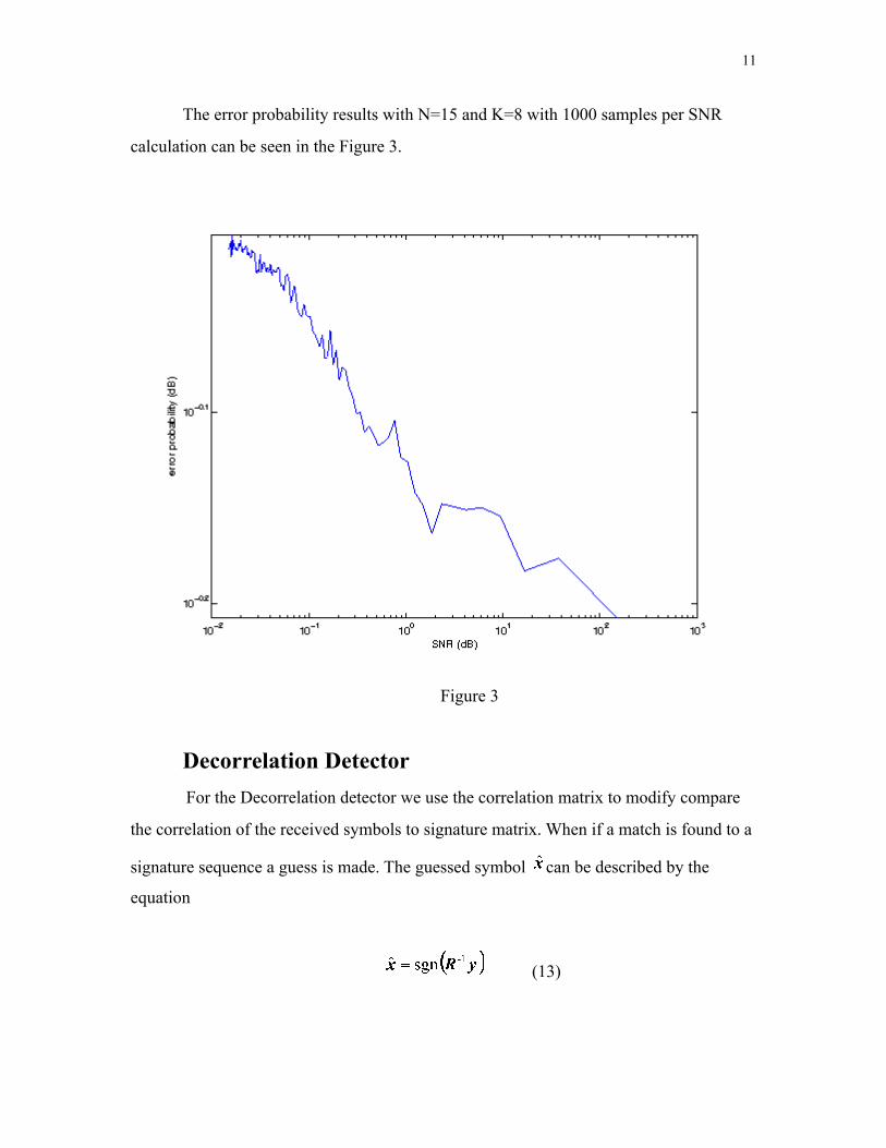
The error probability results with N=15 and K=8 with 1000 samples per SNR

calculation can be seen in the Figure 3.

Figure 3

Decorrelation Detector For the Decorrelation detector we use the correlation matrix to modify compare

the correlation of the received symbols to signature matrix. When if a match is found to a

signature sequence a guess is made. The guessed symbol can be described by the

equation

(13)

11

The detector used the same code as above for determining if the received symbols

matched the true symbol. The SNR calculations for the plots are the same as well. The

error probability results with N=15 and K=8 with 1000 samples per SNR calculation can

be seen in the plot below

Figure 4

Maximum Likelihood Detector The final detector we examined was the ML detector. This detector was different

than the other two as it was much more complex and computation intensive. The guessed

symbol can be described by the equation

(14)

12

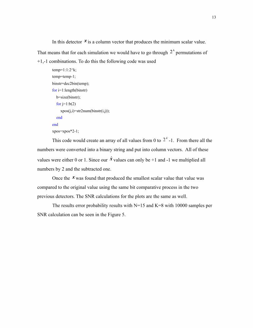
In this detector is a column vector that produces the minimum scalar value.

That means that for each simulation we would have to go through permutations of

+1,-1 combinations. To do this the following code was used

temp=1:1:2^k;temp=temp-1;

binstr=dec2bin(temp);for i=1:length(binstr)

b=size(binstr); for j=1:b(2)

xpos(j,i)=str2num(binstr(i,j)); end

endxpos=xpos*2-1;

This code would create an array of all values from 0 to -1. From there all the

numbers were converted into a binary string and put into column vectors. All of these

values were either 0 or 1. Since our values can only be +1 and -1 we multiplied all

numbers by 2 and the subtracted one.

Once the was found that produced the smallest scalar value that value was

compared to the original value using the same bit comparative process in the two

previous detectors. The SNR calculations for the plots are the same as well.

The results error probability results with N=15 and K=8 with 10000 samples per

SNR calculation can be seen in the Figure 5.

13

Figure 5

The criterion for a positive result is that when the SNR approaches dB the

error probability will be less than dB. By examining the plots of the three detectors

we can see that the ML detector is the only one that comes close to fulfilling this

requirement thus performing the best.

Q FunctionAnother method for predicting the performance of a detector under a specific

signal to noise ratio is to use the Q function. This method uses the fact that we are

considering the noise of our system to be white gaussian noise. Using the definition of a

gaussian distribution, we determine the Q function to be defined by the equation

14

(15)

This mathmatical model shows the idealistic performance of a detection algorithm.

MatLab does not have a Q function command but can approximate the math using the erf

function. For the Multiuser case of the Matched Filter we can show the Q function to be

(16)

The Q function for the other detectors is developed in the same way, using the definition

of the SNR and gaussian distribution. A plot of the simulated performance and the

calculated performance is shown below.

Figure 6

We now have all the tools required to make some very good observations about

the performance of the three detection methods. We can see that the Maximum

Likelihood detector is the “optimal detector” since it has the best response curve. It has

15

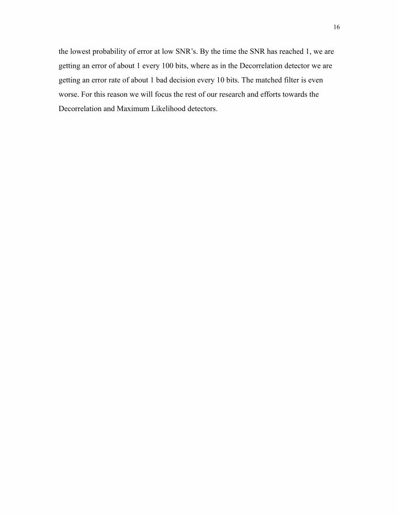
the lowest probability of error at low SNR’s. By the time the SNR has reached 1, we are

getting an error of about 1 every 100 bits, where as in the Decorrelation detector we are

getting an error rate of about 1 bad decision every 10 bits. The matched filter is even

worse. For this reason we will focus the rest of our research and efforts towards the

Decorrelation and Maximum Likelihood detectors.

16

Chapter IV: Complexity vs. Performance

When we talk about the complexity of a detection algorithm, we are talking about

the computational power involved in making a decision about the input and spitting out a

guess on what the transmitted bit was. For the Matched Filter detector, the decision is

made based on the sign o the received signal, therefor the math involved in making the

decision is quite simple. Since the detector is so computationally easy but poor quality,

we will not look into trying to make this detection method better and accept the algorithm

for what it is. Instead we will now investigate the complexity of the Decorrelation and

Maximum Likelihood detectors.

Older versions of MatLab contained the ability to keep track of the number of

floating point operations in a given function. But since the introduction of the LAPACK,

which replaced LINPACK in MatLab, the flops counter command has become obsolete.

Being able to count the number of flops in a program is the best way to determine the

“idealized” runtime and therefor, the complexity of the detection algorithm. But, since the

only tool in MatLab to count the number of floating point operations has been removed,

our team calculated the actual run time of the detection algorithms. This gives rise to

several problems. First, our functions may not be perfectly idealized in the way they are

written and could contain more calculations than are required to properly execute the

detection algorithm. The second problem comes from the fact that some MatLab

functions have odd runtime quirks in them. An example of this is the differences between

the exp() and sqrt() functions. The sqrt() function has 8 flops per calculation, where the

exp() function has 5 times that but has a significantly lower runtime.

For these reasons our method of calculating the runtime of the detetion algorithms

is not the most accurate method for determining their complexity but since the addition of

17

the LAPACK to the MatLab library, the calculation is close enough that we can show the

general trends in their performance and complexity. From the two figures below we see

that the runtimes and the trends in complexity of the Matched Filter and Decorrelation

detector are very similar but the runtime of the later is slightly higher. This means that the

Matched filter detector is a poor detector given that its performance is extremely poor

compared to the Decorrelation detector while it is not much less complex. The Maximum

Likelihood detector on the other hand has a complexity that is much more complex than

the others. For this reason reducing the number of flop counts for this detection algorithm

is the best way to achieve a better detector with less complexity.

Figure 7

18

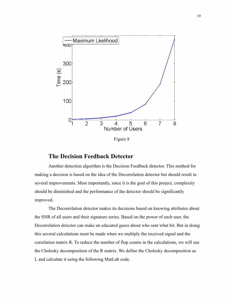
Figure 8

The Decision Feedback DetectorAnother detection algorithm is the Decision Feedback detector. This method for

making a decision is based on the idea of the Decorrelation detector but should result in

several improvements. Most importantly, since it is the goal of this project, complexity

should be diminished and the performance of the detector should be significantly

improved.

The Decorrelation detector makes its decisions based on knowing attributes about

the SNR of all users and their signature series. Based on the power of each user, the

Decorrelation detector can make an educated guess about who sent what bit. But in doing

this several calculations must be made when we multiply the received signal and the

correlation matrix R. To reduce the number of flop counts in the calculations, we will use

the Cholesky decomposition of the R matrix. We define the Cholesky decomposition as

L and calculate it using the following MatLab code.

19

L = (chol(R))';

MatLabs chol() function actually returns the U matrix which is the transpose of the

Cholesky L matrix. So we just transpose the matrix to receive the L Cholesky

Decomposition.

Any square matrix can be written as a lower triangular matrix and its transpose.

This means that the Cholesky decomposition contains enough information about the

power of each user to make the same decision as the Decorrelation detector with less

computations. The difference is we can now make one more adjustment that will improve

the performance of the Decision Feedback detector.

User reordering is important in this detection method. Since one user has a better

signal than another, its signal has the biggest influence in the interference scheme. For

that reason, the user with the highest signal power is the easiest to make a decision about.

To use this phenomenon we implemented an algorithm that determines the user with the

highest power at the receiver and makes a decision on them first, then subtracts their

influence from the received signal. Then we make a decision on the user with the second

highest power and so on and so forth until all users bits have been calculated.

Since we can determine the Cholesky decomposition and new user ordering off

line we can say that the Decision Feedback detector should use slightly less

computational power than the Decorrelation detector and improve the probability of error

curve as well. In our implementation of the program we see that complexity is slightly

higher but this could be for several of the reasons stated earlier about the inefficiencies of

the MatLab programming language. We are unable to control the multiplication of the

upper triangle of the Cholesky decomp matrix which is all zeros so it has no influence, so

this adds floating point operations that do not need to be calculated. We do see an

improvement in performance of the detector, though it is very slight.

20

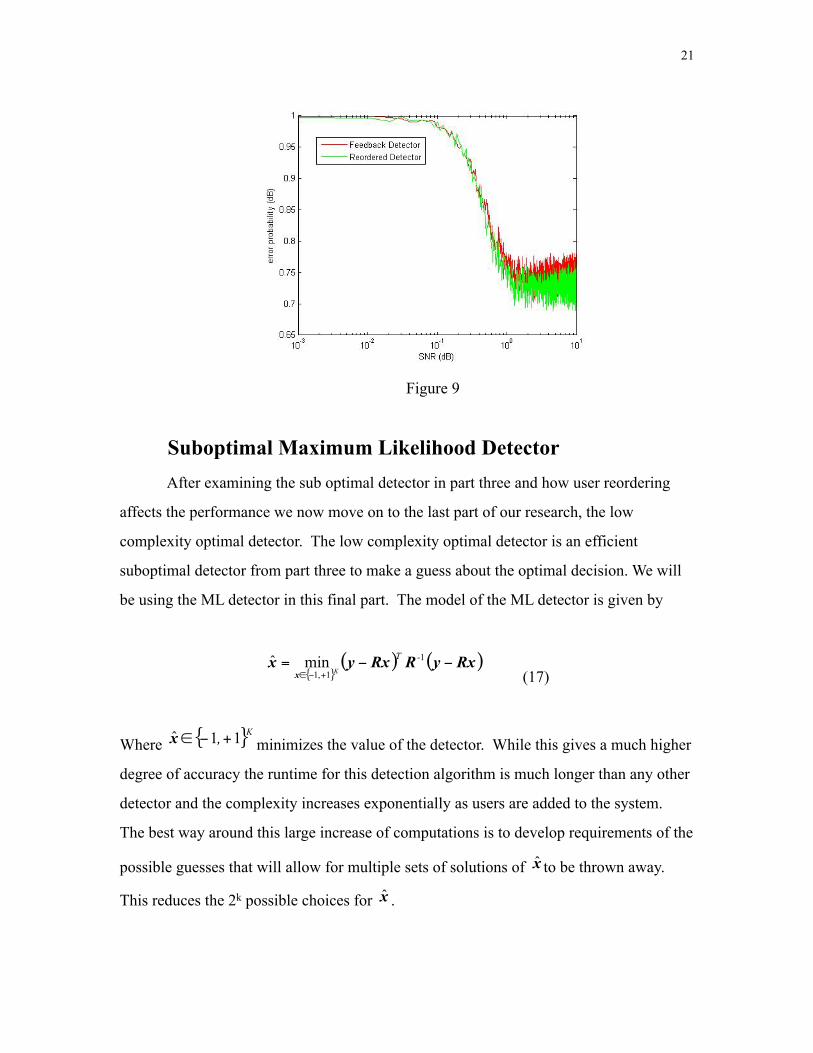
Figure 9

Suboptimal Maximum Likelihood Detector After examining the sub optimal detector in part three and how user reordering

affects the performance we now move on to the last part of our research, the low

complexity optimal detector. The low complexity optimal detector is an efficient

suboptimal detector from part three to make a guess about the optimal decision. We will

be using the ML detector in this final part. The model of the ML detector is given by

(17)

Where minimizes the value of the detector. While this gives a much higher

degree of accuracy the runtime for this detection algorithm is much longer than any other

detector and the complexity increases exponentially as users are added to the system.

The best way around this large increase of computations is to develop requirements of the

possible guesses that will allow for multiple sets of solutions of to be thrown away.

This reduces the 2k possible choices for .

21

These requirements can be found by developing upper and lower bounds on

possible values. With these bounds in place the decision vector can then be narrowed

down before making guesses. These bounds can be found through the use of Cholesky

decomposition. With the reduction of computations that comes from using the lower

triangular matrix we can find the relation between and . From part three with any

given matrix the matrix can be found as

(18)

Where chol() is the Cholsky decomposition function within MATLAB. Now that we

have our relation we can then substitute into our detector. This results is

(19)

And with the matrix identity that we then see that the detector can be

modeled as

(20)

With this simplification we can then derive that if we only know part of our decision

vector , we can then see that our minimum value will be represented by .

Knowing that will minimize our output we can see that .

Now that we know the bounds of what optimal detection are we can start to

design our low complexity optimal detector algorithm. Taking our decision vector and

partitioning it so that

22

(20)

Once the decision vector is portioned we will examine what happens if we only knew .

If contains many errors then will be true and will not lead

to optimal detection since,

(21)

Now that we know cannot be a part of our decision we will then be able to reduce the

possible guesses for detection.

For example, if we have K=10 users then the total possible combinations of

decisions is 1024. If were to represent the first 3 users and we determined that did

satisfy our bounds, then the total number of decisions would be then reduced to 128, a

significant improvement.

23

Chapter V: Future Work

While our team began by striving to understand the 3G cellular networks CDMA

detection methods, it was not our final goal. It was only the first step on the road to

determining a low complexity detection method. Our final goal was to make some

acceptable tradeoffs and modify the Maximum Likelihood detector to hopefully derive an

algorithm for CDMA signal detection that has a relatively low complexity but allows the

probability of a detection error to become slightly worse.

In route to this final deliverable, our team first has a few other tasks that we wish

to accomplish. After studying the Matched Filter detector, which is by far the most simple

yet worst performing detector, and the Decorrelation detector, the middle of the road

detector, we wished to evaluate ways of making these more efficient. Also, our team

examined one last detection scheme called the Decision Feedback detector. Which is

based on the Decorrelation detector and makes its decisions with a little knowledge about

the power and channel gain of each user. We then compared the many different detection

methods, evaluated what makes each detector simple, yet reliable, and apply the

knowledge to discover what might simplify the optimal detector with out to badly

sacrificing output integrity.

After all the research was done, we looked at the ML detector and decided that the

high complexity comes from the number of different evaluations that it has to make.

Based on the number of users, there is a large field of choices that minimizes the error.

For this reason, we decided to find an algorithm that reduced the number of outcomes the

detection algorithm had to choose from. By doing this the detector uses less floating point

operations and is less complex. The problem is that it is not making the guess based on all

the bits in the received signal and therefor sacrifices some of its performance. But based

24

on the needs of the the company running the algorithm, they can choose how much

resolution they need for proper detection. If the users need higher performance on the

detector they can change the number of bits in the list to make the detector have a higher

resolution at the price of slowing the computations down.

Since the demand for an update to the 3G system is required, many companies are

looking for that 4G telecommunications system. Since CDMA is on the way out, this

project maybe dated. Or it may not. If this project has produced a favorable result,

CDMA may still be used for several more years, saving users and companies from having

to abandon their current telecommunication systems.

We, as a team, feel that our projected has been completed to the fullest extent. We

see no need to continue this endeavor further in the upcoming academic year. We have

fully examined all aspects of the CDMA realm and have successfully examined the

complexity and performance of current detection methods. We were able to also examine

ways obtain a detection algorithm that has an acceptable performance while decreasing

the complexity of the detector. From our view all goals of the project have been met.

25

Chapter VI: Conclusions

In the CDMA world there is a growing need for faster, less complex, signal

detection algorithms. In the growing world of wireless telecommunications, bandwidth is

fast becoming a scarce commodity. With millions of users listening to the radio, watching

satellite television, accessing the internet through wireless gateways, and making wireless

phone calls on their cell phones, not to mention the many ways of wireless ad-hoc data

exchange between handheld devices, the air ways are quickly becoming a crowded place

for a communications signal. According to the Cellular Telecommunications & Internet

Association more than 25 million people became cell phone users in 2005, bringing the

total to 207.9 million wireless phone users in the United States alone.2 With outdated

technology such as FDMA, which radio communications use, the available bandwidth

has become extremely limited.

With the development of the CDMA access scheme users are able to more

efficiently share bandwidth but at a price. Detection of a single user in any scheme is

relatively simple, but when you have multiple users sending information at the same

frequency, separation of data becomes complex. In fact, to reliably determine a single

users signal out of many becomes a very in depth process. For the more simple detection

schemes discussed in chapter 3, detection is simpler, but does not necessarily meet the

user’s demand of high quality output. Especially at lower SNR’s where the probability of

detection error is greater than the more complex optimal detector. With the growing

enigma of more and more users, detection becomes more and more complex requiring

faster, higher power, more expensive computing machines.

26

2 Annual Report and Analysis of Competitive Market Conditions With Respect to Commercial Mobile Services retrieved 10 Dec 2007.

The average consumer demands higher speeds at twice the quality for half the

price. When this becomes a customer’s specification for a product, the complexity of the

system sky rockets. To combat the complexity issue some compromises need to be made.

In the course of the project so far, our team has discovered that when more users occupy

the bandwidth, complexity rises. When we want a lower probability of error at a given

SNR, complexity rises. With the before mentioned problem of more users occupying the

same bandwidth, we have noticed some tradeoffs must be made.

At a minimum our project, has evaluated the need for a less complex CDMA

signal detection scheme. By evaluating telecommunication system needs and user

demands, we have explored different techniques to make some acceptable tradeoffs and

develop a low complexity signal detection algorithm which does not completely sacrifice

its performance.

27

References

1. J. Rockey Luo, “Biography”. http://www.engr.colostate.edu/~rockey/ 10 Dec 2007

2. S. Verdu, Multiuser Detection. New York: Cambridge University Press, 1998.

3. P. Peebles, Probability, Random Variables. New York: Irwin/McGraw-Hill, 2001.

4. S. Haykin and M. Moher, Introduction to Analog & Digital Communications. USA: John Wiley & Sons, 2007.

5. Annual Report and Analysis of Competitive Market Conditions With Respect to Commercial Mobile Services, WT Docket No. 05-71, FCC 05-173, released Sept. 30, 2005

28

Appendix A - Abbreviations

x - Defined as the user’s transmitted bit in the single user case

x - Is a column vector where xk is the kth user’s transmitted bit

- Defined as the output of the detector in the single user case (the detectors “guess”)

- Is the output of the detector in the multi user case (a column vector of the detectors “guesses” where k is the detectors guess of the kth user’s transmitted bit)

w - Defined as the power of the users transmission in the single user case

W - Is a k x k diagonal matrix where wk is the kth user’s transmission power for the multi user case

h - Defined as the channel gain for the user in the single user case

H - Is a k x k diagonal matrix where hk is the kth user’s channel gain for the multi user case

n - Defined as the Gaussian noise distribution in the channel for the user in single user case

σ - Defined as the variance of the noise

v - Is a Gaussian noise column vector N bits long

s - Is a column vector signature sequence of the user in the single user case

S - Is an N x k matrix where the columns are the corresponding user’s signature series for the multi user case

R - Is an N x N matrix defined by R = ST*S for the multi user case (for best case R = N*I when the user’s signature sequences are orthogonal to each other)

A-1

y - Defined as the signal at the receiver (channel output) for the single user case

z - Is a column vector or matrix, for the single user and multi user cases respectively, of signals received at the channel output

y - Is the matched filter output the receiver computes to determine the transmitted signal of the users where yk is the kth users transmitted signal

I - Defined as the Identity Matrix

k - Defined as the number of users in the channel

N - Defined as the signature series length

ML - Stands for Maximum Likelihood (also referred to as the optimal detector)

SNR - Stands for Signal to Noise Ratio

3G - Stands for 3rd Generation (usually refers to third generation cellular networks which work on the current CDMA detection algorithms)

L - Cholesky Decomposition of R

y - L-T*y is just a notional simplification

ζ - Is an auxiliary vector

zk - Another axiliary vector associated with each k

A-2

Appendix B - Budget

The Low Complexity Signal Detection design project is rather straight forward. Our projects goal is primarily research and simulation based; our team has not made much spending this year. Our project is significantly research and simulation into current signal detection techniques and simulate their performance using MatLab, which is graciously provided by Colorado State University. Our only expenses this year were for the E-Days presentation. We used many print credits through the University and needed to purchase more. Also, we had to purchase presentation materials required for the competition. Our project accrued very slight expenses that totaled a meek $20.

B-1

Acknowledgements

We would like to acknowledge Dr. J. Rockey Luo, our advisor. His help and advice is what got us this far. Dr. Luo has been there when we have had questions and is always willing to take time out of his day to explain the minute details of the project and our assignments. Thank you, Rockey we appreciate you sharing you wisdom with us.

I