loudspeaker equalisation to compensate for low …€¦ · school of physics msc in acoustics and...
TRANSCRIPT

University of Edinburgh
College of Science and Engineering
School of Physics
MSc in Acoustics and Music Technology
Final Research Project: Dissertation
Loudspeaker Equalisation to Compensate for Low Frequency
Room Acoustics
Simon Hendry
s0569270
Abstract
This project looks at the theory of low-frequency room acoustics and methods of compensating for the effects of room modes and speaker placement in the small studio. The generation and a comparison between the sine sweep and maximum length sequence for use as a test signal is discussed with the exponential sine sweep emerging as a more effective test signal for quiet room scenarios. An intelligent filter is designed to flatten the frequency response of a room modeled on recordings taken in specific listening places within that room. A program was written to apply this filter to a sweep along with the chance to change variables controlling various techniques to improve both the quality and accuracy of the results. This filter can then be exported as a .WAV file containing an impulse response to be used in conjunction with a convolution reverb plug-in. This program was then tested in a range of environments with varying degrees of success.

2
DECLARATION
I, Simon Hendry, confirm that this dissertation and the work presented in it are my
own achievement.
1. Where I have consulted the published work of others this is always clearly
attributed.
2. Where I have quoted from the work of others the source is always given. With the
exception of such quotations this dissertation is entirely my own work.
3. I have acknowledged all main sources of help.
4. If my research follows on from previous work or is part of a larger collaborative
research project I have made clear exactly what I have contributed myself.
5. I have read and understand the penalties associated with plagiarism.
Signed:
Matriculation Number: s0569270
Date:

3
Table of Contents
1. Introduction ............................................................................................................................ 5
2. Room Acoustics ..................................................................................................................... 5
2.1 Reflection and Diffraction ............................................................................................... 6
2.2 Normal Modes ................................................................................................................. 7
3. The Experiment .................................................................................................................... 11
3.1 Generating Test Tones ................................................................................................... 11
3.1.1 Sine Sweep Generation ........................................................................................... 12
3.1.2 Maximum Length Sequence Generation ................................................................ 14
3.2 Comparison Between Sweep and MLS Measurements. ................................................ 16
3.3 Frequency Correction..................................................................................................... 18
3.4 Real-time ........................................................................................................................ 18
4. Experimental Procedure ....................................................................................................... 21
5. Results .................................................................................................................................. 23
5.1 Anechoic Chamber......................................................................................................... 23
5.2 Studio 2 .......................................................................................................................... 25
5.3 Improvements to the Model ........................................................................................... 31
6. Testing Further Environments ............................................................................................. 35
6.1 Graphic EQ .................................................................................................................... 36
6.2 Alison House Postgraduate Sound Lab.......................................................................... 37
6.3 Alison House Studio 4 ................................................................................................... 38
6.4 Alison House Russolo Room ......................................................................................... 39
7. Discussion, Improvements, and Other Methods .................................................................. 41
7.1 Floating-point accuracy ................................................................................................. 43

4
7.2 Amplitude Modulation ................................................................................................... 44
8. Smoothing Mini-investigation ............................................................................................. 51
9. Conclusion ........................................................................................................................... 54
10. Bibliography ...................................................................................................................... 55
11. Appendix ............................................................................................................................ 56
11.1 ECS Matlab Code ........................................................................................................ 56
11.2 Amplitude Envelope Correction Code ......................................................................... 61
11.3 MLS Generation Code ................................................................................................. 64

5
1. Introduction
Every leading loudspeaker manufacturer likes to boast that their speakers have a ‘flat’
frequency response. Essentially, this means that the speaker outputs all frequencies with
equal power. In reality, this is extremely improbable due to the mechanical design of the
speaker and the nature of the crossover if the speaker possesses more then one driver; so
companies specify that their speakers are, for example, flat from 20 to 22000 Hz ±3 dB. This
means that the power of each frequency outputted stays within a 3 dB band around the ideal 0
dB line between 20 Hz at the low end and 22 kHz in the high treble.
So why do we spend so much effort and money on creating a ‘flat’ speaker? For an audio
engineer, it is essential for you to hear exactly what your mix sounds like. This way there will
be no surprises when it comes to being played on laptop speakers or a car stereo system.
Unfortunately for the engineer, the manufacturer’s specification of 20 Hz to 22 kHz ±3 dB
may hold true in the anechoic chamber (something I plan to verify later on) but as soon as the
speaker is placed in a room, there are many more variables that will affect the perceived
frequency response of the speaker. The aim of this project is to identify and investigate some
of these variables and design a filter to correct the imperfections of the frequency response,
regardless of what room the speaker is placed in. To fully understand how a room can alter a
speaker’s frequency response, some knowledge of basic room acoustics is needed.
2. Room Acoustics
Room acoustics, or the scientific study of how sound behaves in a room, is relatively new in
the field of scientific research with Wallace Sabine conducting the first acoustical analysis of
the Boston Music Hall in 1900 (Thomson, 2003). In context, this is just four years after the
discovery of radioactivity and five years before Albert Einstein published his paper on special
relativity. Since then, many people have written papers and books on the subject and
acoustics is now at the forefront of scientific research. A benchmark book on room acoustics
entitled ‘Room Acoustics’ was written by the German Professor Heinrich Kuttruff in 1973. In
this book, Kuttruff discusses the idea of room modes. These modes are frequencies that ‘fit’
exactly into a room and thus are more prominent in that room. Such room modes would
definitely modify the perceived frequency response of a loudspeaker if placed in the room.
He also discusses the reflection of sound from various surfaces, another factor which would

6
alter the frequency response of our speaker if it was placed close to a wall or corner. Here I
will briefly summarise the physics behind these two acoustical phenomena.
2.1 Reflection and Diffraction
Sound waves are reflected and diffracted in the same way light waves are, except diffraction
can occur with objects many times bigger for sound as the wavelengths of sound are several
orders longer then those in the visible spectrum of light. In an ideal rectangular room, sound
would only be reflecting off flat surfaces so the law of reflection states that the angle of
incidence is equal to the angle of reflection. This is not so straight forward when we start to
introduce parabolic surfaces. If however the sound is travelling towards a corner, the wave
will be reflected twice and return back in the same direction as the approach regardless of the
incident angle:
Figure 1: Waves are always reflected in the direction of incidence when approaching a
90° corner (Everest, 2001:244).
Generally, the speakers face away from any walls or corners, so why is this such a problem?
The answer lies in the diffraction of the sound caused by the loudspeaker itself. The effects of
diffraction are most prominent when the wavelength of the wave being diffracted is similar or
larger than the object that it is passing. The frequencies f=100 Hz to f=500 Hz correspond to
wavelengths λ=3.44 to λ=0.688 meters, based on the speed of sound in air to be 344 ms-1
.
Thus a speaker is going to cause considerable diffraction effects to the sound being produced
by it; furthermore the lower frequencies are going to be affected more then the higher
frequencies. It is this exact phenomenon that makes the placement of the subwoofer in any

7
arrangement from a small home cinema system to touring rock rigs a relatively inexact art as
the sound will diffract around any objects in the way to reach your ears (an exception to this
of course is placing the woofer in a corner as this will help excite all three types of room
mode which I will discuss in the next section).
It then follows from a combination of the above two effects that the bass response of a
speaker will be heightened considerably if the speaker is placed close to a wall or corner of a
room, regardless of which direction the speaker is facing due to low frequencies being
emitted towards the wall or corner:
Figure 2: Speaker cabinet diffracting low frequencies into a reflective surface.
Further reading on speaker edge diffraction can be found in John Vanderkooy’s paper A
simply theory of cabinet edge diffraction (Audio Engineering Society v.39 issue 12 p923-
933). Further reading on radiation from sources near walls or corners can be found in
Acoustics – An introduction to its physical principles and applications by Allan Pierce
(chapter 5: Radiation from sources near and on solid surfaces).
2.2 Normal Modes
For the following room mode calculation, we shall consider a rectangular room of dimensions
(x,y,z). Not only is this usually the shape of the studio or listening room, it will also simplify
the mathematics massively. We will also assume that the walls are rigid and have an
absorption coefficient, α, of 0. The wave equation may be written in Cartesian coordinates as:
02
2
2
2
2
2
2
pk
z
p
y
p
x
p
(1)

8
Where p is the sound pressure and k is the wave number (Kuttruff calls it the propagation
constant). The solution to this equation can be separated, thus we can split up the pressure
into its three factors:
)()()(),,( 321 zpypxpzyxp (2)
This splits up equation (1) into three ordinary differential equations, one for each dimension.
For instance, the equation for the x-dimension would be:
01
2
2
1
2
pkdx
pdx
(3)
We can then apply the properties that the boundary conditions introduce. As the room mode
frequencies fit exactly into the dimensions of the room, we can say that at the boundaries (i.e.
at x=0 and x=Lx for the first dimension) the pressure must be at a maximum, thus the
derivative of the pressure with respect to x must be zero:
01 dx
dpfor x=0 and x=Lx (4)
Let us consider the general solution to equation (3):
)sin()cos()( 111 xkBxkAxp xx (5)
There of course holds two analogous equations for p2(y) and p3(z). The constants A and B are
chosen to satisfy the boundary conditions so we can see immediately that B1=0 as
cos(kx*0)≠0. The derivative is given below:
0)cos()sin( 111 xkkBxkkA
dx
dpxxxx
(6)
Now considering the other boundary of x=Lx, we can see, again using the derivative, that:
0)(sin1 xxx LkkA (7)
Thus x
xx
L
nk
for nx=0,1,2,3… (8)
Again, similar allowed values for ky and kz can be calculated in the same fashion. Using the
relationship between frequency and wave number, the allowed frequencies can be given by:

9
zyxzyx nnnnnn kc
f2
(9)
Or to rewrite it in a more useful form:
222
2
z
z
y
y
x
x
L
n
L
n
L
ncf where nx,ny,nz=0,1,2,3,4… (10)
Any mode in this set of frequencies therefore is labelled and governed by the integer set nx,
ny, and nz. The modes in a room can be categorised into three types depending on these
integers. An axial mode has only one non-zero integer, thus the wave propagates along an
axis perpendicular to the other two axis of the room. A tangential mode has two non-zero
integers, for example, a wave between two corners of a room but still perpendicular to the
third axis. An oblique mode has three non-zero integers. Such a wave would travel between a
top corner of a room to the opposite bottom corner. It follows then that the combined effects
of room modes will be most prominent in a corner of the room where all three types of modes
are excited. Bellow is a table of the frequencies of room modes for a room measuring
3.1x4.1x4.7m:
Figure 3: Room modes for a room measuring 3.1x4.1x4.7m (Kuttruff, 1973:53).
We can see that as the mode frequencies increase, they also become closer together. By the
time the frequencies reach around 400 Hz, they are so close together that they are no longer
distinguishable.
O. J. Bonello, an acoustics consultant from Buenos Aires devised a method for creating the
dimensions of an ideal listening environment. He subdivides the low end of the audible
spectrum into bands, each ⅓ octave wide (to approximate the critical bands of the human ear)
and then considers the number of modes present in each band below 200 Hz. To meet the

10
Bonello Criterion, each band should have more, or an equal number of modes than the band
preceding it. There are many room dimensions that satisfy this rule, however a smooth graph
of modal density against frequency will yield the best results. Below is such a graph for a
room measuring 15.4x12.8x10 ft:
Figure 4: Graph of density of room modes per ⅓ octave satisfying the Bonello criterion
(Everest, 2001:349).
As well as building the ideal room to reduce the effect of resonant modes, other methods
have been developed, such as the Helmholtz resonator, which absorbs specific frequencies
depending on its design, and the exact placement of absorbing materials such as acoustic
foam. I am going to attemt to try and solve the problem of room modes not by absorbing
them in the room but by modifying the frequency response of the speakers themselves so they
output less power at the problem frequencies.

11
3. The Experiment
The aim of this experiment is to send test tones out of a speaker and then record the test tones
through a microphone placed in various places around the room. A median can be calculated
from these positions and the frequency response of the room can be generated using the fast
Fourier transform. This frequency response should show clearly the problem frequencies in
the low end due to room modes or speaker placement. The experiment can then be repeated
with a filter, designed from the inverse of the frequency response, applied to the test tones
and the resulting response should be flat. If successful, the filter could be applied to a
realtime feed thus making an engineer’s speakers true regardless of the room he is listening
in.
3.1 Generating Test Tones
Traditionally, to investigate the acoustic properties of a reverberant chamber, an impulse was
created using non-electroacoustic methods such as firing a pistol or popping a balloon
(Muller, 2001:32). These methods did create an impulse but they were unlikely to be as
precise as a one-sample long rectangular window which we know to have a flat frequency
response when acted upon by the Fourier transform. There is also a lack of consistency in
these non-electroacoustic methods which make reliability and error calculations highly
unstable. The accepted method therefore is to generate tones digitally to be played through a
loudspeaker to ensure accuracy and repeatability. However, playing an impulse through a
loudspeaker has its drawbacks; apart from being potentially damaging to the speaker
membrane and electromagnetic components of the speaker, it is also unlikely that the speaker
will output a perfect Dirac’s delta function but will output a narrow curved window, similar
to a sync function with damped oscillations both before and after the main peak:

12
Figure 5: Dirac’s theoretical delta function compared to sync function observed when
an impulse is fed through a loudspeaker.
It is suggested that this sync shape is due to the limiting bandwidth that is used. Any limit in
the bandwidth will create a trapezoid shape in the frequency domain, which itself becomes
this sync-like function in the time domain (Farina, 2007).
Any test signal that we do use however has to be both spectrally flat over all frequencies
being investigated and at least as long as the expected impulse response for the space. For
this investigation, I will generate and test two varying types of signal; a sine sweep signal and
a maximum length sequence.
3.1.1 Sine Sweep Generation
With the interest of room modes in mind, it would be convenient to create a signal with more
energy at lower frequencies as the low-order room modes tend to reside between 20 Hz and
200 Hz for an averaged sized studio listening room. More energy in the lower frequencies
will yield more accurate results in this range, and to satisfy this, we could create a sine sweep
whose frequency is increased exponentially between two specified bounding frequencies. In
his paper on sweep measurements, Muller discusses two methods of sweep synthesis. A sine
sweep can be generated in both the time domain and the frequency domain with advantages
and disadvantages to both methods. However, Muller uses a loop based step frequency
implementation for the sweep signal in both domains. I will create my sweep signal using a

13
vector approach (Berdahl & Smith, 2005:10). The exponentially increasing sine sweep from
angular frequency w1 to w2 over a time of T seconds is given by:
)]1(sin[)( / LfsneKns (11)
Where
1
2
1
lnw
w
TwK and
1
2lnw
w
TL
A crucial step in the sweep implementation is to repeat the sweep and record the room
reflections on the second sweep. This is to ensure that all the reflections at all the frequencies
get recorded. Consider the following diagram:
Figure 6: Scenario in which the sweep signal would have to be repeated to record all
relevant acoustic data of the room.
Say that the frequency played at time A only reaches the microphone at time B, which is
perfectly valid as the time of the reflection is still less than the length of the sweep. In this
scenario, the sound of the reflection would not be recorded unless the sweep is repeated and
the recording runs throughout the two sweeps. The second half of this recording should now
possess all the possible reflected sound data and can be carried forward to be processed.

14
3.1.2 Maximum Length Sequence Generation
Maximum length sequences (MLS) are pseudo-random binary sequences consisting of
apparently random 0’s and 1’s. The sequence is spectrally flat over all frequencies except for
the DC and Nyquist frequencies (Kemp, 2002). MLS signals have a huge advantage over
white noise (which is also spectrally flat) as they can be generated and regenerated precisely
and thus there is no unpredictability due to the randomness that white noise possesses.
An MLS signal can be generated by using a feedback shift register consisting of a group of m
binary memory elements per line where m is the order of the MLS. The length of the MLS
signal is given by 2m
-1. The easiest and most computationally-efficient way to generate the
signal is using a recurrence relation which is directly related to the primitive polynomial of
degree m.
For example, let’s take the primitive polynomial for m=5:
1)( 25 xxxh (12)
This is the equivalent of a recursion relation:
iii aaa 25 (13)
Every time the time-step is increased, the group of memory elements shifts one step to the
right and the left-most element is produced by the above recursion relation. As the signal
contains every possible combination of 0’s and 1’s for a five-member sequence (apart from [0
0 0 0 0] as a one would never be generated), the values of the starting memory elements does
not affect the overall sequence. Here are the first six elements of and MLS signal for m=5
with the first memory element [1 1 1 1 1]:
Time Step, i Elements
(ai+4,ai+3,ai+2,ai+1,ai)
MLS signal (ai)
0 11111 1
1 01111 1
2 00111 1
3 00011 1

15
4 10001 1
5 11000 0
6 01100 0
Figure 7: First six elements of an MLS signal for order m=5.
To get the memory elements for the second row for example, the first row gets shifted to the
right, and then the left element is given by ai+2+ai from the row above. Care must be taken to
do modulo-2 addition (the numbers ‘wrap around’ when they reach 2, for example 1+1=2=0,
0+1=1). The final step is to rewrite the 0’s as -1s so the binary sequence is now made up of
1’s and -1’s. As the sequence needs to be at least as long as the room impulse response, I will
use an MLS signal of order m=16, corresponding to a signal length of 216
-1 or 262123
samples, roughly six seconds at a sample rate of 44.1 kHz. Below is a table of recursion
relations for m=1-20 (Stahnke, 1973):
Figure 8: Recursion relations for m=1:20 (Kemp, 2002).
As with the sine sweep, the MLS is doubled in length before it is played. Both the sine sweep
and the MLS signals were created in Matlab.

16
3.2 Comparison Between Sweep and MLS Measurements.
In his paper Transfer-Function Measurement with Sweeps (Muller, 2001), Muller discusses
some advantages and disadvantages of the sweep and MLS methods. The crest factor is an
important concept for test tones as it is the ratio of peak to RMS voltage, or how efficiently a
signal can be transferred from the digital domain through a speaker into the room in testing.
The ideal crest factor is 1; the peak voltage and RMS voltage are the same. The MLS signal
theoretically has a crest value of 1, however in practice, the rectangular wave form changes
considerably as suggested in section 3.2. In particular, the anti-aliasing filters used in DA
converters causes the realistic power of the MLS signal to overshoot the theoretical signal:
Figure 9: The effect of an anti-aliasing filter on an MLS signal (Muller, 2001:24).
The example above has a crest factor of 7.76 dB, meaning the signal has to be fed into the
DA converter at least 7.76 dB below the maximum gain the converter can process for the
filter to act linearly. The sine sweep has a crest factor of 3.01 dB so is favoured over MLS
signals for its larger sound to noise ratio. An experiment to deduce the frequency response of
an analogue tape player was also conducted with both MLS and sweep methods (Muller,
2001:24). The results show that at high frequencies, the MLS signal has considerably more
noise, possibly due to its susceptibility to time-variance:

17
Figure 10: Frequency response of an analogue tape player using MLS (left) and sine
sweep (right) (Muller, 2001:26).
Distortion also affects both sweep and noise-based signals. This usually occurs not from the
surroundings but by the speaker itself. For a noise-based signal such as the MLS, this
distortion component will be distributed evenly over the entire duration of the response. A
longer response time would be one work-around for reducing the effect of distortion, but at
large orders of MLS (order 25 would produce a sequence 12 minutes and 41 seconds long at
44.1 kHz) the signals become more susceptible to time variance resulting in noisy responses
discussed above.
With a sweep however, you have the advantage of being able to entirely isolate any harmonic
distortion after the impulse response has been acquired as it appears as a response at negative
time if you take your direct path to occur at t=0. For example, consider a linear sweep that
progresses at 1 kHzs-1
. At t=100 ms, the sweep will pass through 100 Hz with a second order
harmonic distortion at 200 Hz. When the excitation signal is compressed to an impulse, the
200 Hz harmonic will be treated with a -200 ms delay leaving it present at -100 ms after the
deconvolution. This holds for all other harmonic distortion so it can be easily eliminated by
ignoring any negative time reflections in the impulse response.
In conclusion, the sweep measurement has a lower crest factor resulting in a higher energy
signal, is less susceptible to time-variance reducing the amount of noise in a response and can
be treated to easily eliminate distortion. These three characteristics make the sine sweep an
ideal signal to test room acoustics.

18
3.3 Frequency Correction
The equalisation filter applied to the test sweep (and ultimately any signal outputted by the
speaker) is modelled on the inverse of the system response which we obtain by the recorded
signal. Say the room boosts a specific frequency, f1 by 3 dB, the filter we apply to the output
will aim to lower that same frequency f1 by 3 dB. The following flow chart explains the steps
of the filter design:
Figure 11: Process for creating a correction filter to counteract the room modes.
For the filter to counteract the effects of the room, we need M(w), the final signal heard at the
listening position to be the same as the original sweep, S(w). The filtered signal N(w) that we
send out the speakers is now defined as:
)(
)(
)(
)()(
2
wX
wS
wH
wSwN
(14)
Note that all the calculations are done in the frequency domain. This is to minimise
computing power as multiplication (in the frequency domain) is more computationally-
efficient then convolution in the time domain.
An inverse Fourier transform can then be performed on N(w) to convert this desired response
back to the time domain.
3.4 Real-time
The next step is to take this filter and see how it can be created as a recursion relation for
implementation in real time. Presently, the filter can only be applied to a piece of pre-

19
recorded audio (in the test case, this audio is the exponential sine sweep). Furthermore, the
filter and the piece of audio have to possess the same number of samples. In reality, this is not
very convenient as we want to be able to apply the filter constantly to any audio leaving our
computer’s sound card. The aim of this section is to transform the filter into a format where it
can be used in real-time. The simplest way to achieve this is to create a recursion relation, for
example the nth
sample of the filtered signal contains a bit of the nth
sample of the original
signal as well as a bit of the previous sample, and a bit of the sample before that and so on:
...321 nnnnn DxCxBxAxX (15)
The coefficients A, B, C… are to be determined.
The most straight forward way to find a recursion relation of a filter is to find the impulse
response in the time domain. Schroeder used cross-correlation to compute the impulse
response (Schroeder, 1979). This had various drawbacks, including the fact that the MLS
signal is 2m
-1, and for the radix-2 fast Fourier Transform algorithm to work, the length of the
signal needs to be a power of 2 (Hsu, 1996:11). Schroeder originally overcame this problem
by interpolating an extra sample to match the requirements of the radix-2 FFT. This cross-
correlation calculation is still computationally inefficient and it was not until Schroder was
aware of developments in Hadamard Spectroscopy done in the early ‘70s that he could use
the Hadamard transform to efficiently calculate the impulse response from an MLS signal
based recording. More on the Hadamard transform can be found in Hsu (1996:12-16).
To create an impulse response from a sweep signal, deconvolution is used. This can be
thought of as division in the frequency domain of the dry signal and the recorded signal. The
dry signal is ‘subtracted’ from the recorded signal in the deconvolution process leaving just
the acoustical effects of the room. In our case, we do not want an impulse response of the
room, but an impulse response of our correction filter. A block diagram can be helpful to
understand this more clearly:
Figure 12: Process for filtering a real time signal

20
We can see that the signal to be played through the speakers, N’ is defined as:
)(
)()('
)(
)(')('
wX
wSwS
wH
wSwN (16)
Therefore the filter that we apply to our live signal is S(w)/X(w). This division is our
deconvolution described above, and by taking the inverse fast Fourier transform of this, we
get an impulse response. This response can be used with any convolution reverb plug-in such
as SIR (www.knufinke.de) for windows or Space Designer (www.apple.com/logicstudio) for
mac. Such programs simply convolve an impulse response with a real-time input signal to
add the reverberant characteristics of the room where the impulse response was obtained.
21
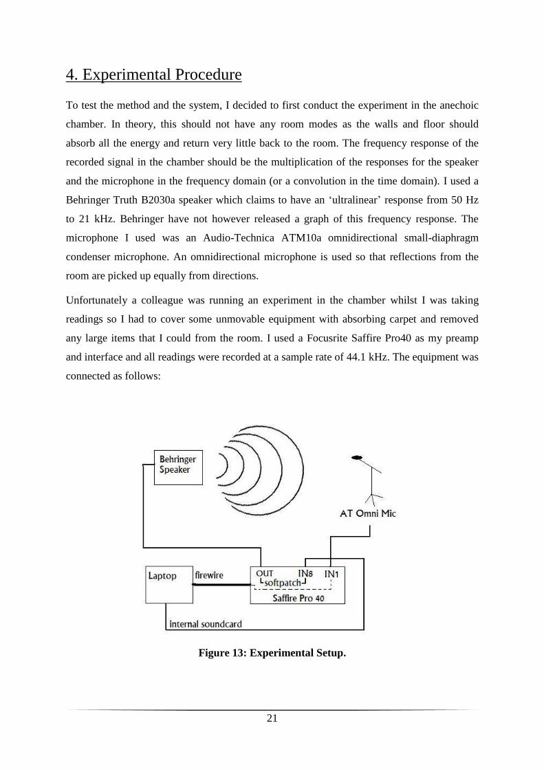
4. Experimental Procedure
To test the method and the system, I decided to first conduct the experiment in the anechoic
chamber. In theory, this should not have any room modes as the walls and floor should
absorb all the energy and return very little back to the room. The frequency response of the
recorded signal in the chamber should be the multiplication of the responses for the speaker
and the microphone in the frequency domain (or a convolution in the time domain). I used a
Behringer Truth B2030a speaker which claims to have an ‘ultralinear’ response from 50 Hz
to 21 kHz. Behringer have not however released a graph of this frequency response. The
microphone I used was an Audio-Technica ATM10a omnidirectional small-diaphragm
condenser microphone. An omnidirectional microphone is used so that reflections from the
room are picked up equally from directions.
Unfortunately a colleague was running an experiment in the chamber whilst I was taking
readings so I had to cover some unmovable equipment with absorbing carpet and removed
any large items that I could from the room. I used a Focusrite Saffire Pro40 as my preamp
and interface and all readings were recorded at a sample rate of 44.1 kHz. The equipment was
connected as follows:
Figure 13: Experimental Setup.

22
Matlab refuses to play and record simultaneously through an external sound card, a problem
which is well documented on the MathWorks website and has no simple solution. I therefore
routed the sweep to the interface via my laptop’s internal soundcard. This was then patched
internally to the speaker. The signal from the microphone was directed via firewire back to
my laptop and recognised as originating from a separate soundcard. I positioned the
microphone at a distance of two meters from the speaker and the microphone recorded the
output from the speaker simultaneously to it being played. The second half of this recording
was then used as both signals were repeated as discussed earlier. For the sine sweep, the
discrete Fourier transform (DFT) was undertaken using Matlab’s fft command. This was then
divided by the Fourier transform of the original signal in order to normalise the large amount
of bass energy created by using an exponential sweep. The absolute value of this complex
vector can then be converted to decibels using the following equation:
)(log20 10 powerdB (17)
This vector can then be plotted against a frequency vector to give the frequency response of
the anechoic chamber.
Similarly the absolute value of the DFT of the MLS recorded signal can be converted into
decibels and plotted as a frequency response. The peak of the response is arbitrary and
depends largely on the amount of gain supplied by the preamp in the Saffire Pro40. As the
decibel scale is purely relative to a reference point (in our case undefined) the graph can be
shifted in the y-axis at will. I chose the median value of the frequency response to represent 0
dB so that the graph fluctuates evenly below and above the x-axis. Three sine sweeps and
three maximum length sequences were recorded and processed by Matlab.
I then proceeded to take the setup to studio 2 in the basement of the JCMB. This space
measures 2.21x3.07x3.06 meters and the walls are covered with plasterboard. The speaker
was placed on a stand in the middle of the shortest wall and responses for 9 different
microphone positions were recorded including one position with the microphone exactly in
the middle of the room. One response was also recorded for the speaker in a bottom corner of
the room with the microphone diagonally opposite to try and capture the largest amount of
room modes.

23
5. Results
5.1 Anechoic Chamber
The results from the anechoic chamber were not as flat in the frequency domain as expected.
In the range from 50-400 Hz, both the sine sweep and the MLS signal generated a flat
response at the microphone to ±5 dB, however as the frequency increased, there were more
fluctuations in the response. These higher frequency fluctuations are most lightly caused by
reflections off the metal grill floor, the metal microphone stand or the plastic rails.
Figure 14: Low frequency response in the anechoic chamber by sweep (above) and MLS
(below).
-80
-70
-60
-50
-40
-30
-20
-10
0
10
0 100 200 300 400
Gai
n /
dB
Frequency /Hz
Graph of frequency against gain for a sweep signal in the anechoic chamber
Sweep 1
Sweep 2
Sweep 3
-80
-70
-60
-50
-40
-30
-20
-10
0
10
20
0 100 200 300 400
Gai
n /
dB
Frequency /Hz
Graph of frequency against gain for an MLS signal in the anechoic chamber
MLS 1
MLS 2
MLS 3

24
The graphs in figure 14 each contain the three repeat tests so we can see due to the overlap
that the consistency of the results is very high from 50 Hz and above. The sweep’s starting
frequency was set to 50 Hz as the speaker acts non-linearly below this frequency so the data
below 50 Hz can be discarded. The response in the chamber is not exactly flat; however there
are no narrow peaks that suggest room modes. The wide peaks that we can see in Figure 14
may be caused by the responses of the test equipment such as the speaker, microphone and
preamps. We can see that even though to a listener, the sweep and MLS signal sound vastly
different, both graphs have the same features so it is assumed that the MLS signal was
generated correctly and is indeed spectrally flat.
It is not until we approach the higher frequencies where we can really see a difference
between the sine sweep signal and the MLS signal. Figure 15 shows a logarithmic plot of the
frequency response in the anechoic chamber using the sweep (above) and the MLS (below):
Figure 15: Full range frequency response of the anechoic chamber using sweep (above)
and MLS (below).
We can see that even in the full bandwidth of the experiment, both methods share similar
characteristics in the response; however the MLS signal contains a lot more noise between
2000 Hz and 20000 Hz as predicted in section 3.2. Even though the responses are similar in
the low-frequency range that we are interested in for room mode compensation, the

25
correction filter is designed using the full range response. For this reason, the sweep
technique will be carried forward to test more reverberant rooms.
The acoustics of the anechoic chamber provide the simplest case for the correction technique
as the response is already relatively flat between 50 and 400 Hz. A Matlab script was written
to compute the steps involved in the correction from Figure 9. Below is a graph of the
original sweep response along with the same sweep having been filtered by the correction
filter:
Figure 16: Frequency response of the anechoic chamber measured with a sine sweep
before and after the correction filter.
We can see that the filter does indeed act against the combined natural acoustics of the room
and equipment and makes the response recorded at the microphone spectrally flat to ±1 dB in
the range from 50 Hz to 400 Hz. If the engineer wants to preserve the characteristics of his
favourite microphone for a recording, the response of the microphone can always be found in
the anechoic chamber, and then compensated for in the final correction filter.
5.2 Studio 2
To start with, the room modes were calculated in this space using equation (10). Figure 17
shows a graph of the first 64 modes:
-50
-40
-30
-20
-10
0
10
0 50 100 150 200 250 300 350 400
Gai
n /
dB
Frequency /Hz
Graph of sweep response before and after correction filter
Sweep recording
Corrected sweep recording

26
Figure 17: First 64 room modes of Studio 2 in the JCMB.
This data was used to see if the space satisfied the Bonello Criterion discussed in section 2.2.
Figure 18 shows a graph of frequency against room mode density:
Figure 18: Graph showing room modes per frequency band for Studio 2 in the JCMB.
We can see that the ratio of dimension lengths in this space do not satisfy the Bonello
Criterion as there are less modes in the 6th
frequency band than the band preceding it,
therefore we may expect some very prominent modes and non-consistent responses in the
room.
The extent to which the room affected the frequency response was immediately clear as the
responses obtained in Studio 2 were considerably less consistent over the full range compared
to the responses measured in the anechoic chamber. The following graph shows the
frequency response for all nine microphone positions between 50 and 400 Hz:
0 100 200 300 400Frequnecy /Hz
Graph of Room modesAxial Modes
Tangental Modes
Oblique Modes
0
2
4
6
8
10
12
14
16
18
0 50 100 150 200 250 300
Ro
om
mo
de
de
nsi
ty /
(1/3
)oct
ave
ban
d
Frequency /Hz
Bonello Crieterion - Graph of frequency against room mode density

27
Figure 19: Frequency response from 50 to 400 Hz in Studio 2 for nine microphone
positions.
A straight line was fitted to the data from -60 dB to the value at 50 Hz. As the speaker does
not function linearly under this frequency, we are not able to modify the response by applying
a filter so the data is expendable. For each set of data, the 0 dB reference was chosen to be at
the median of the response vector. We notice that not only do the responses for each
microphone position vary largely over the frequency range but they also are not consistent
with other positions. These fluctuations are most lightly caused by reflections from objects in
the room such as the air conditioning duct, window sill and door handle, thus the effect of
these reflections is going to change as the position of the microphone is varied.
Having said that the response varies from position to position, there are similarities in the
characteristics of the plots, especially in the lower end of the spectrum. We can clearly see
common peaks around 58, 80, 115 and 160 Hz. These peaks are more lightly to be caused by
room modes rather then reflections as they are consistent and independent of microphone
position.
To investigate the effect of room modes on the average response of all the microphone
positions, the room modes of the space were plotted against a graph of the median of all nine
microphone positions at ear level. A 20-point moving average was used to smooth the graph:
-60
-50
-40
-30
-20
-10
0
10
20
30
40
0 50 100 150 200 250 300 350 400
Gai
n /
dB
Frequency /Hz
Frequency against Gain in Studio 1 for ten microphone positions
position1
position2
position3
position4
position5
position6
position7
position8
Centre

28
Figure 20: Graph of smoothed average frequency response with room mode
frequencies.
The room modes line up well with the peaks and troughs of the response, with the single axial
modes in the bass and the groups of modes around 180 and 230 Hz standing out in particular.
A small investigation into different methods of smoothing is included later in this project.
Having established that this room is certainly not ideal to listen in due to its large fluctuations
in the lower register response due to room modes, it should be a good test for the correction
script to see if the results are as convincing as they were in the anechoic chamber.
Figure 21 shows a graph of frequency against gain for one single microphone position with
the original recording and also the corrected recording:
-60
-50
-40
-30
-20
-10
0
10
20
0 100 200 300 400
Gai
n /
dB
Frequency /Hz
Graph of average frequency response and room modes against gain
moving average frequency response
room modes

29
Figure 21: Frequency response of Studio 2 both before and after the correction filter.
We can see that the affect of the correction script successfully flattens out the response to
within ±3 dB in the frequency range 50-400 Hz. The success of the correction filter on the
response relies, as expected, massively on the position of the microphone. Figure 22 shows
the response of the recorded corrected sweep with the microphone as above and also the
response when the microphone is moved just 30cm to the right in the room:
Figure 22: The effect on frequency response due to a shift in microphone placement by
30cm.
-60
-50
-40
-30
-20
-10
0
10
20
30
0 50 100 150 200 250 300 350 400
Gai
n /
dB
Frequency /Hz
Frequency against Gain for uncorrected and corrected sine sweeps
original sweep recording
corrected sweep recording
-60
-50
-40
-30
-20
-10
0
10
20
30
0 50 100 150 200 250 300 350 400
Gai
n /
dB
Frequency /Hz
Effect of microphone position on correction response
Original microphone position
Microphone position moved by 30cm

30
We can see that the results generally agree with one another up to around 250 Hz. Above this
frequency, small fluctuations in microphone position have an increasing effect on the
perceived response of the room as the frequency increases. We can see from Figure 20 that
there is a large number of room modes around 250 Hz so this could contribute to the drastic
change in response above this frequency between the two microphone positions. To
overcome this, we need to compromise on frequency response and consistency over the area
of the room. We can design a filter based on the median response of the nine microphone
positions found above and apply this filter to the sweep in the hope that a compromised
response is created. Figure 23 shows the response of the room with the median response used
as the basis for the correction filter:
Figure 23: Using the median of nine microphone positions does not flatten out the
frequency response.
We can see straight away that the results are barely an improvement on the original responses
recorded in Figure 19. By averaging the positions, we seam to be averaging out the very
peaks that define the room and make the filter work. This doesn’t mean however that the user
cannot define listening points of interest; a technique used by IK multimedia
(www.ikmultimedia.com) in their ARC software. The engineer can save the mixing position
as a ‘sweet spot’ as well as a sofa, for example at the back of the studio. By selecting either
the mix position or the sofa from a drop-down menu, the sweet spot will change position in
the room.
-80
-60
-40
-20
0
20
40
0 100 200 300 400
Gai
n /
dB
Frequency /Hz
Frequency response of Studio 2 after a correction filter based on the median of nine
microphone positions was applied

31
5.3 Improvements to the Model
The graphs of the correction filter for single positions show that the room modes can indeed
be compensated for by a correction filter and that the system and method are generally very
successful. Graphs alone however do not portray the sever colouring that the filter had on the
sweep sound. After the filter is applied, the sweep no longer sounds like a single sweep but a
distant sweep with a dominating bell sound in the foreground. Moreover these bell sounds
change pitch depending on the microphone position in the room. Further inspection of the
signal in the frequency domain shows the lightly cause of these tones. The 1/X(w) term in
equation (16) yields high sharp peaks in the frequency response of the filtered signal if the
original response was close to zero as near-zero terms tend towards infinity when inverted.
Figure 24 shows the response of the inverse filter where you can clearly see these peaks
which colour the sweep:
Figure 24: Frequency response of the inverted recorded sweep with circled dominant
peaks.
These peaks are going to be present in our final filter (fft(sweep)/fft(recorded sweep)) and it
is these peaks that are causing the bell tone effect. Two techniques were implemented to try
and reduce the drastic effect of these peaks. Firstly a threshold was introduced to leave any
data below said threshold unaffected and to rewrite any data above with the threshold value.

32
This works in a similar way to a compressor with a very harsh knee and an ∞:1 ratio. Care
was taken to preserve the angle of the complex data when those values above the threshold
were rewritten as this phase information will be crucial to the inverse Fourier transform
algorithm. Figure 25 shows two sharp peaks being reduced by the threshold filter along with
a plot of the inverse filter in the frequency domain. There is also a significant amount of
energy approaching the Nyquist frequency. This could be caused by the filter trying to
compensate for the natural high frequency roll off in the response of all speakers. The filter is
effectively trying to boost frequencies which the speaker is not able to produce. This high
energy in the filter reduces the proportional amount of energy at lower frequencies so when a
normalisation was performed, the sweep seemed very quiet. The threshold filter overcomes
this problem by eliminating these high energy frequencies. The threshold value, expressed as
the allowed increase in decibels from the minimum gain has to be adjusted for each
microphone position or room for the best results:
Figure 25: Sharp peaks being truncated at the threshold gain (left) and the inverse filter
with very high energy approaching Nyquist (right).
Secondly the data was smoothed via convolution with a cosine window. The window was
written to be conjugate symmetric and the length of the active section of the window, m,
controls the amount of smoothing that the filter will undergo. The window was also divided
by its sum so that the energy spread over the whole window is one. This is effectively a
normalisation in the frequency domain and will stop the convolution affecting the gain of the
filter. Care was taken to convolve the window with the absolute value of the response in
order not to try and average complex numbers. Again the phase data was conserved:

33
Figure 26: Smoothing window with m=20 (left) and effect of smoothing on the response
(right).
This technique successfully smoothes the graph but it also smoothes some of the peaks that
make the filter work. Tests show that a small window length in the order of 1-5 samples
produced a sweep that was more spectrally flat but still contained overpowering peak
frequencies resulting in bell tones. As the window length is increased, the sound quality of
the sweep is slightly improved however the response diverges from the ideal flat response.
Whilst analysing the room impulse response, small amounts of distortion were observed at
the very end of the response. I decided to try and eliminate this to improve the overall quality
of the filter. The distortion occurs at the end of the response due to the harmonic distortion
being produced at negative time (discussed in section 3.2) being ‘wrapped around’ during the
deconvolution process. Figure 27 shows a close up look of the room impulse response. We
can see that the fluctuations here are at Nyquist frequency:
Figure 27: Distortion present at the end of the room impulse response.

34
To eliminate this distortion, the last 50 samples of the impulse response were replaced with
zeros. The response was then transformed back to the recorded sweep by a convolution with
the original sine sweep. This modified, non-distorted recording was then taken forward to the
correction section of the program. Careful adjustments of threshold value, window length and
the number of samples to erase from the end of the impulse response will yield the best
results.
The experiment was repeated with these improvements and the full range response was
analysed. A listening test verified that the bell tones had indeed been reduced by the
improvements to the model however they were still present.
The creation of the sweep, application of the filter and the corrections discussed above were
written into one single Matlab script with a graphical user interface and the option to change
all the variables used and view graphs of the pre and post frequency response both smoothed
and unsmoothed, the room’s impulse response, the correction filter’s impulse response and
the correction filter in the frequency domain pre and post smoothing and threshold. Figure 28
shows a screen shot of the GUI:
Figure 28: GUI created in Matlab of the Equalisation Correction System.

35
The variables can be tweaked until the user is happy with both the audio quality of the
corrected sweep and the new established frequency response. There is then an option to write
a .wav file containing the impulse response of the correction filter for use with a convolution
reverb plug-in.
6. Testing Further Environments
With a full working program of my equalisation correction system, I tried to test the software
in as many different environments as possible starting of with the environment inside my
Saffire pro40 firewire interface as the effects of this unit will add to the effects of any
speakers or microphones connected to it.
Figure 29: Frequency response, impulse response and correction filter for the Saffire
pro40 interface.
We can see that the frequency response of the interface is practically flat as expected. The
high roll-off begins at around 17 kHz but is extended to over 21 kHz with the filter applied;
the high shelf trying to compensate for this roll-off can be seen in the bottom right graph.
There is a sharp dip just above 20 kHz which the correction filter as over-compensated for.

36
The peak responsible for correcting this dip is circled in the filter response graph. The
impulse response is sharp, again as expected and the high frequency fluctuations either side
of the main peak are caused by the anti-aliasing filters inside the unit. The peak is at 746
samples corresponding to a 16.9 ms latency.
6.1 Graphic EQ
The program was then run through a 15 band graphical equaliser to see if the filter could
flatten out an applied EQ. The 400 Hz band was set to +12 dB and the 1000 Hz band to -12
dB. We can clearly see the effects of the EQ on the pre-filter response and again the filter
succeeds in compensating for these effects and reducing the unit to a flat response. The dip
just above 20 kHz is identical to that of the previous experiment so we can deduce that this is
a product of the interface and not of the EQ unit. The latency of this system is surprisingly
shorter then the standalone interface at 16.1ms. This suggests that the latency of the interface
is dependent on internal computer factors such as available RAM and instantaneous CPU
usage:
Figure 30: Responses for 15 band graphic EQ with +12 dB at 400 Hz and -12 dB at 1
kHz.

37
6.2 Alison House Postgraduate Sound Lab
The sound lab is a large rectangular room with no acoustic treatment. Tests were run using an
AKG 414B microphone set to omnidirectional and a Genelec 1032A bi-amplified speaker.
Results were recorded with the microphone positioned at a distance of 1 meter (the Genelec
specifications state that any near-field effects of listening to two drivers should be
unnoticeable at any distances greater than 0.7 m:
Figure 31: responses for the sound lab in Alison House at a distance of 1 meter.
We notice that the delay on the direct signal in the room’s impulse response has risen to 880
samples, an increase of 134 samples from the results for just the interface. A time of 134
samples corresponds to 3ms or a propagation of 1.04 meters so these results agree well with
the predicted results for this microphone position. We can also see that the filter impulse
response is very involved as it’s trying to compensate for multiple reflections around this
large room. The result of this is a deep colouring of the sweep with rings starting to be heard
again.
A second set of results were recorded for the microphone positioned in the middle of the
room. In this scenario, the program has to flatted out a frequency response many times worse
then any small to medium sized studio listening room (see figure 32). We can see
confirmation of the large room acoustics in the room impulse response which has many more
peaks then the previous examples corresponding to more prominent room reflections. This

38
takes its toll on the sound quality with a very distorted sweep being the outcome of the filter
and we can see from the zoomed plot that the program struggles to flatten out the response,
particularly at low frequencies:
Figure 32: Responses for the sound lab in Alison House in the centre of the room.
6.3 Alison House Studio 4
Studio 4 is a small rectangular room with sound absorption panels on many walls and corners
in attempt to create a good listening environment. The reference monitors in this studio are
small twin-driver (4” and 1”) passive speakers made by Blue Sky as part of their MediaDesk
5.1 system. The speaker frequency response is 110 Hz to 20 kHz ±3 dB and again the AKG
414B microphone was used to record the signals. The microphone was placed in the listening
position at ear level so this test is the closest yet to an everyday implementation of the
program.

39
Figure 33: Responses for Studio 4 in Alison House.
We can see that the impulse response is very clean, due to the acoustical treatment in the
room. The correction filter is also relatively flat with a small rise approaching Nyquist which
was reduced with the threshold function. A small amount of smoothing was also used in this
room with the outcome being a very good sounding sweep with a flat frequency response. We
do notice in the top graph that there is some noise in the low frequencies. This is caused by
the filter trying to correct frequencies below which the speaker is designed to function
linearly.
6.4 Alison House Russolo Room
The Russolo room is similar in size and proportion Studio 4 with some acoustic treatment in
the form of carpet boards (compared to absorbing foam in Studio 4). The room impulse
response suggests that either the positioning of the carpet boards or the material itself is not
as effective as in Studio 4 as a strong second reflection can be seen. The room is equipped
with Genelec 1030A speakers with a frequency range of 55 Hz to 18 kHz ±2.5 dB. Figure 34
shows the results for this space:

40
Figure 34: Responses for the Russolo Room in Alison House.
The original response in this room is more consistent then any other room tested. This could
be due to the combination of quality, full range speakers and an acoustically treated room
which we have not come across yet. The result of this is a filter with few correction peaks; in
fact the largest peak in the correction filter is trying to compensate for the dip around 20 kHz
created by the interface. The room response confirms the high roll-off in the speakers at 18
kHz and with the filter applied, the response remains linear until 20 kHz.

41
7. Discussion, Improvements, and Other Methods
My first comment on this program would be that as it stands, it can not turn any room into a
perfect listening environment; moreover it seams that the software makes the listening
experience in an already bad room even worse, even if it creates a flat response theoretically.
The program works at its best when used in a room which has already been acoustically
treated. In such a room, the program takes an already reasonably good response and makes it
close to perfect without the need to introduce bell-tones. A further investigation could be to
look at the level of response where the program starts to make an improvement to the sound
quality rather then diminishing it.
The fact that the sweep does not cover the whole frequency range from 1 Hz to Nyquist does
pose some problems which were identified in the interface response test. The response was
much more stable over the full range then for 40-20000 Hz which was the bandwidth used for
testing all the speakers. Using the full range of frequencies on loudspeakers however could
potentially damage them as forcing high energy low frequency (1-15 Hz) tones tend to burn
out the electromagnetic components of the speaker.
Another problem with this software is that it naturally reduces the volume of the input signal
due to large energies outside both the range of human hearing and most loudspeakers. If our
ears could detect frequencies up to 22050 Hz, we would hear this frequency dominating any
signal after the filter has been applied to it (use of the program with very high end speakers
which have a linear response in this region is not recommended around household pets!). To
overcome this problem, the filter could be programmed to only work in a specified range, for
example from 50 Hz to 18 kHz. This could be achieved by replacing any data outside this
range in the recorded sweep with the original sweep. When the filter is then convolved with
the signal in question it should be unaffected in the frequencies outside the predefined range.
Another side effect of the loss in gain is that when the filtered signal is being tested for the
new frequency response, fewer room modes are excided due to less energy being emitted
from the speaker. This is going to reduce the effects of the space towards those experienced
in the anechoic chamber, thus the new recorded frequency response appears much flatter than
it is in reality.
An interesting further investigation would be to code an intelligent parametric equaliser with
a limiting band of frequencies. This program could search the frequency response for high

42
peaks and note their frequencies and gains. A parametric EQ could then be designed to target
only these frequencies. This method would surely result in a high quality, low accuracy filter
which would sound better then the technique employed in this investigation. A parametric EQ
however would not contain the same level of detail, and by increasing the allowed number of
bands to increase the detail of filter, the results will tend towards the form of the filters
designed by the above method. It would be interesting to see however the quality of results
when limited to, for example, ten bands.
Due to all the above problems, this software could not be used in its present state in a
professional environment as the sound quality is unacceptable. To fix this, we really need to
eliminate any traces of the bell-tone features in the corrected sweep. A relatively straight
forward way to reduce the ringing is to window the filter correction impulse response. Many
of these impulse responses were oscillatory (the bottom right plot in Figure 31 for example)
as the filter was trying to reverberate specific frequencies. This often resulted in correction
impulse responses that were as long as the sweep itself, which when used in conjunction with
a convolution reverb, is going to return these bell tones strongly. If the correction impulse
response was windowed to a length in the region of 0.1-0.3 seconds, the ringing may be
considerably reduced. The effect of this however would surely be a less flat corrected room
response:
Figure 35: Windowing the filter impulse response may reduce the presence of ringing.
Another possible test could be to generate the sine sweep in the frequency domain (Muller,
2001:36-39) mentioned in section 3.1.1. Using this sweep as the test tone could result in a
different compensation filter which does not introduce bell tones. Building the sweep in the
frequency domain introduces the idea of a group delay, τG(f); the time at which a particular

43
frequency is delayed from the start of the signal. The group delays for a linear sweep are
quite straight forward:
2/)0()
2()0()(
Fs
fFsf GGGG
(17)
Here, the group delay of frequency f is the delay of f=0 Hz (usually zero) plus the group delay
of Nyquist (usually the duration of your sweep) multiplied by the desired frequency as a
fraction of Nyquist. For example the group delay of 11025 Hz in a sweep lasting 10 seconds
will occur at 0+(10*¼)=2.5 seconds as expected. The calculations involved in the group
delays of a logarithmic sweep are slightly more involved:
)(log 2 fBAG (18)
Where )(log)( 2 startstartG fBfA and )/(log
)()(
2 startend
startGendG
ff
ffB
These equations have the ability to specify the start and end frequency to match the
application in which they are being used. The phase of the sweep is proportional to the group
delay via the following expression:
)()((2)()( fdfdfff G (19)
With NFsdf 2/
This set of magnitude and phase data can be converted into real and imaginary parts like any
complex number:
biabercomplexNum
phasemagnitudeb
phasemagnitudea
)sin(
)cos(
(20)
An inverse Fourier transform can then be performed on the vector τG to create the sweep in
the time domain.
7.1 Floating-point accuracy
It occurs to me that the above improvements and suggestions to create a working filter should
not be needed as my implementation should work theoretically; the presence of sharp peaks

44
in the filter which we perceive as bell tones are only present because the response in the room
at those specific frequencies is extremely quiet. There is no reason theoretically for my
program to over-compensate for these features in the response by creating such strong
frequency peaks. It was suggested to me that there might be a problem in the bit-depth
accuracy as a result of the floating-point method of accuracy that is implemented by Matlab.
A simple example of the drawbacks of using floating-point accuracy can be demonstrated my
asking Matlab to compute 0.1+0.2-0.3, with the resulting answer being 5.5511x10⁻¹⁷
. Matlab
uses floating-point accuracy to be able to express a wider range of numbers. Take for
example a five decimal digit accuracy. In fixed-point system can represent the numbers
12345, 123.45, 0.0012 and so on. A floating-point system on the other hand has the freedom
of choosing where the decimal point is placed. Such a system can represent numbers like
123450000000 (1.2345x10¹¹
) or 0.00012345 (1.2345x10⁻⁴
). Using such a versatile system
however slightly reduces the accuracy of mathematical operations such as multiplication and
addition (as proven above). The fact that floating-point operations cannot truly mimic correct
arithmetic operations causes some surprising accuracy problems. In the case of filter design, a
small discrepancy in the accuracy of a point in the order of 10-4
can have considerable
consequences when inverted. A brief analysis of my results shows that many of the rooms
had multiple values in the absolute frequency response in this order of magnitude. This
program would have to be run on a platform which uses fixed-point accuracy to determine if
these discrepancies in accuracy have had any significant effect on the outcome of the filter.
7.2 Amplitude Modulation
With the realisation that I was not going to be able to test the theory of floating-point
accuracy, I was determined to create a clean-sounding sweep with a flat response. Another
method to achieve this is to control the amplitude of an input signal depending on its
instantaneous frequency. The input can be broken into consecutive short windows similar to
the design of the phase vocoder. These windows would be typically 128 or 256 samples in
length. The frequency response of each individual window can then be compared with the
frequency response of the room obtained by the methods used above and if the window
contains any room modes identified by sharp peaks in the room frequency response, the
amplitude of that particular window can be reduced accordingly. The most straight forward
method to test this hypothesis is to create a sweep and analyse the amplitude envelope of the
recording. This amplitude envelope can then be inverted and applied to the sweep once again.
This method looks similar to above but here we do not enter the frequency domain as part of

45
the filter process (we do enter it as part of the analysis). The restriction of this method
however is that this particular test will not work in real time; moreover it will only work
when applied to a sweep as the sample number should be directly related to the instantaneous
frequency and the sweep only contains one single frequency at any given time.
The amplitude envelope can be constructed by taking the maximum value from the recorded
signal within each cycle. A Boolean was used to find the local maxima for each cycle by
comparing its amplitude with samples immediately before and after. Figure 36 shows a
section of the sweep in the time domain along with the points for the local maxima:
Figure 36: Graph of a section of sine sweep with the local maxima for each cycle
identified using a Boolean command.
It became apparent that the first portion of the recorded sweep has to be smoothed very
slightly to overcome multiple maxima in one cycle:
Figure 37: Smoothing is needed to avoid the calculation of multiple local maxima within
one cycle.

46
The smoothing could only be performed on a portion of the low frequency sweep as it would
act as a low pass filter if applied to any high frequency cycles.
Once restricted to one local maximum per cycle, the set of maxima was written to an array
consisting of sample number in one column and amplitude in another column. A straight line
interpolation was then performed using the number of samples between successive maxima
and the difference in amplitude recalled from the array:
Figure 38: Graph of amplitude envelope with a section of sine sweep showing the effects
of linear interpolation.
The envelope was then smoothed via a convolution with a cosine window and shifted in the
negative x direction to compensate for the delay in the system. This delay comes from both
latency in the interface and the time it takes for the pressure waves to travel from the speaker
to the microphone. The amount of shift was calculated from the room’s impulse response.
The maximum of the absolute value of the response within the first 10000 samples was
calculated and its sample number used to shift the amplitude envelope so that it will line up
with the sweep being played. The maximum was taken from the first 10000 samples to try
and avoid the maximum being taken from any harmonic distortion at the end of the impulse
response.
The original sweep should have an amplitude of one for all the cycles. Say, for example, a
cycle in the recorded sweep has an amplitude of 0.6. This corresponds to a loss of 40% to the

47
room. We then require the filtered sweep to have such an amplitude that when 40% is
removed from it, the resulting amplitude is one. This is achieved by inverting the interpolated
amplitude envelope and then performing a vector multiplication with the original sweep.
Similar to the results from the original compensation filter, the corrected sweep is reduced
greatly in volume. A graph of the inverted amplitude envelope shows that again, there is a
disproportional amount of energy approaching Nyquist which will reduce the relative gain at
other frequencies when normalised:
Figure 39: Graph of the inverted amplitude envelope showing a dominant proportion of
energy above the human hearing threshold, reducing the gain of the audible section of
sweep.
As with the above filter correction method, a threshold is applied to the envelope, in this case
a maximum allowed amplitude. Any values below 0.01 were also replaced with 0.01 to try
and avoid large peaks appearing in the inverse envelope.
The program was implemented in a medium sized bedroom studio with a Mackie MR5 active
monitor (60 Hz – 20 kHz ±3dB) and an SE electronics 4400a omnidirectional microphone.
Figure 40 shows the frequency response of the sweep before and after the envelope filter,
along with a zoomed plot of original sweep, recorded sweep, amplitude envelope, inverted
amplitude envelope and corrected sweep:

48
Figure 40: Room responses before and after envelope correction (top) and
implementation of the method on a section of sweep (bottom).
The response of the room after the envelope filter had been applied is a marginal
improvement but not nearly as convincing as frequency filter based correction above. We can
see from the detailed plot that all the vectors have been correctly implemented; the red
amplitude envelope successfully follows the contours of the green recorded sweep. Likewise
the purple corrected sweep follows the contours of the turquoise inverted envelope. The
problem lies here with the phase difference between the original and corrected sweeps and
the recorded sweep. The latency calculation was supposed to line up the sweeps, but here we
can see, most predominantly in the sharp peak in the inverted envelope, that it is not being

49
applied to the correct cycle of the original sweep. This could be due to the unreliability of the
assumption that the maximum value of the impulse response is also the latency value. On
some runs, the impulse response does not seam to possess and obvious direct-path peak and
on others, a second reflection is calculated as being stronger then the direct path.
A new method to more accurately determine the latency was devised by calculating the
instantaneous frequency of each cycle by the difference in sample number between
concessive zero-crossing points with negative gradient for both the original sweep and the
recorded sweep. This data was written into an array and then compared. Figure 41 shows the
first 24 rows of the array along with a plot of the difference in sample number for the original
and recorded sweep:
Figure 41: Raw data and plot of the difference in sample number of successive negative
zero-crossings for both original and recorded sweep.
We can see here that the instantaneous frequency of the recorded sweep is not consistent and
as the differences can be matched up for certain cycles, the two sweeps quickly lose their
phase agreement. Implementation of code for a computer to automatically line up the two
sweeps therefore is extremely hard. One test was run with the two sweeps being lined up by
human calculation and judgement. Figure 42 shows the results:

50
Figure 42: Responses before and after the correction envelope with human alignment of
the original and recorded sweep.
The envelope does improve the spectrum up to around 12 kHz confining it to ±4 dB. Above
this frequency however, the envelope makes no visible improvement to the response.
Alignment at such a high frequency is hard and detail may be lost using a linear interpolation
when the consistency of the amplitude envelope is low. In conclusion, a filter of this design
should theoretically create a flat response and a clean sounding sweep but there is a loss of
accuracy by designing the filter on local maxima points which occupy less than 0.1% of the
sweep data in comparison to the frequency-based filter which is designed using all the data
points of the sweep.

51
8. Smoothing Mini-investigation
Towards the beginning of this project, I was getting some very questionable results when
using a smoothed signal. I decided to conduct a small investigation into the cause of this and
to test some different types of smoothing. When displaying a frequency response, it is often
more important to see the general shape of the sound rather then the details of many
insignificant minor fluctuations. Below are two frequency responses obtained from
www.audioholics.com:
Figure 43: Room frequency response (left) with the same response post-smoothing
(right).
Both plots have the same general shape yet it is easier for us to look at the smooth graph and
deduce information about the response of the room. Muller suggests in his paper on
measurement techniques (Muller, 2001) that a convolution with a Hann window would
smooth the graph. This essentially is a moving average with a centred weighting as a
convolution steps through the vector one sample at a time and the Hann window is bell-
shaped thus vertically symmetrical. When this method was implemented however, the graph
was successfully smoothed with the length of the Hann window determining the amount of
smoothing, however the process also affected the magnitude data; the wider the window, the
larger the magnitude of the peaks became. To investigate this phenomenon and to see if a
simple division to rescale the data could solve the issue, 14 different window sizes from 4
samples to 56 samples were convolved with a random noisy signal. The windowed amplitude
was plotted for six frequencies:

52
Figure 44: Amplitude against window length for 6 sample numbers.
For each frequency, a trend line in the form of a 6th
order polynomial was added. We can see
that there is a correlation between window length and amplitude but this correlation changes
with frequency and is defiantly not a straight line. To investigate further, a graph of the
original signal smoothed with seven window lengths were plotted on the same graph:
Figure 45: Convolution with various length Hann windows and their effect on
frequency peaks.
0
0.2
0.4
0.6
0.8
1
1.2
1.4
1.6
0 10 20 30 40 50 60
Am
plit
ud
e
Window Length
Graph of window length against amplitude for 6 frequencies
10000th sample20000th sample30000th sample40000th sample

53
Here we can clearly see the raising of amplitude as the window length increases; convolution
with the Hann window seams to create large peaks from a seemingly flat original signal. We
also see that the window shifts the frequency of the peaks to the right. Even if the window
was normalised to solve the increasing gain, the shift in frequency will certainly be a
problem. It seams that the window length, coupled with the un-smoothed height of a peak
relative to the data previous to the sample in question, is related to the frequency that the
graph is shifted. As the frequency data is crucial to our filter design, a convolution with a
Hann window will not suffice.
A more straight-forward moving average was then tested. Each sample, Xn, was calculated as
the mean of the samples Xn-9:Xn+10 creating a 20-point moving average. Data from the first
nine and last 10 samples are unaffected. Figure 44 shows the frequency response of Studio 2
with and without a moving average being applied:
Figure 46: 20-point moving average applied to the frequency response of Studio 2.
The moving average acts successfully as a smoothing function on the graph removing some
intensity out of the main peaks but still preserving their position whilst smoothing out many
of the minor fluctuations in the response that may be caused more by near-field reflections
then room modes.
I finally tried a convolution with half a cosine cycle as a window as designed in section 5.3
and used in my final program. This window acts as a non-linear centre-weighted moving
average without shifting the frequency peaks.
-70
-60
-50
-40
-30
-20
-10
0
10
20
0 50 100 150 200 250 300 350 400
Gai
n /
dB
Frequency /Hz
Effect of 20-point moving average on a frequency response from Studio 2
Raw response
20-point moving average

54
9. Conclusion
The aim of this project was to create a filter that when applied to the output of a speaker,
creates a flat frequency response over the speaker’s active range. Both the exponential sine
sweep and the maximum length sequence were examined and analysed for use as a test tone
with the sine sweep emerging as the more appropriate signal for this application. A filter was
constructed in the frequency domain modelled on the inverse of the recorded sweep and the
application of this filter was found to create an ultra-linear response. The response was found
to be highly position dependent and using a median of multiple positions did not improve the
response. The quality of the response is also very poor and coloured with ringing tones. The
use of a threshold gain and smoothing on the filter reduced the presence of the ringing but the
filter is still not ideal for any practical application. Various further methods and
improvements to the filter were discussed including creating a limited band parametric
equaliser and the possibility of running the program on a platform that uses fixed-point
accuracy instead of floating-point accuracy. Finally a correction envelope modelled on the
amplitude of each cycle within the sweep was created and tested with disappointing results.
The accuracy used to develop this sweep was not of a high enough resolution to be effective
at high frequencies.
Although I have not managed to create a working compensation filter of good sound quality
in this project, I am convinced that the theory covered is a strong starting point and that
creating a full working compensation filter is definitely achievable.

55
10. Bibliography
Berdahl, E., & Smith, J. (2005). Transfer Function Measurement Toolbox.
Everest, F. (2001). Master Handbook of Acoustics. McGraw-Hill.
Farina, A. (2007). Advancements in impulse response measurements by sine sweeps. Audio
Engineering Society , 3.
Hsu, K. (1996). Simulation of Room Acoustics. Undergraduate Thesis, University of
Queensland.
Kemp, J. (2002). Theoretical and experimental study of wave propagation in brass musical
instruments.
Kostek, B. (1999). Soft Computing in Acoustics. Heidelberg: Physica-Verlag.
Kuttruff, H. (1973). Room Acoustics. Applied Science Publishers LTD.
Muller, S. (2001). Transfer-Function Measurement with Sweeps. Audio Engineering Society ,
443-471.
Pierce, A. D. (1991). Acoustics - An introduction to its physical principles and applications.
New York: Acousticl Society of America.
Schroeder, M. R. (1979). Integrated-impulse method measuring sound decay without.
Acoustical Society of America , Vol 66 p497-500.
Stahnke, W. (1973). Primitive Binary Polynomials. Mathematics of Computation , volume
27.
Thomson, E. (2003). History of Acoustics. Architectural Science Review , Vol. 46.
Vanderkooy, J. (1991). A simple theory of cabinet edge diffraction. Audio Engineering
Society , 39 (12), 923-933.
I would like to acknowledge Dr. Jonathan Kemp for his patience and
guidance throughout this project.

56
11. Appendix
11.1 ECS Matlab Code
function varargout = ECS2(varargin)
% Begin initialization code - DO NOT EDIT gui_Singleton = 1; gui_State = struct('gui_Name', mfilename, ... 'gui_Singleton', gui_Singleton, ... 'gui_OpeningFcn', @ECS2_OpeningFcn, ... 'gui_OutputFcn', @ECS2_OutputFcn, ... 'gui_LayoutFcn', [] , ... 'gui_Callback', []); if nargin && ischar(varargin{1}) gui_State.gui_Callback = str2func(varargin{1}); end
if nargout [varargout{1:nargout}] = gui_mainfcn(gui_State, varargin{:}); else gui_mainfcn(gui_State, varargin{:}); end % End initialization code - DO NOT EDIT
% --- Executes just before ECS2 is made visible. function ECS2_OpeningFcn(hObject, eventdata, handles, varargin)
handles.Fs=44100; %sample rate handles.f1=40; %start frequency handles.f2=22050; %end frequency handles.N=16; %order of the signal handles.threshRange=600; %range of min to max value for threshold in dB handles.m=22050; %window length for smoothing of inverse filter
expressed as a frequency handles.n=100; %window length for smoothing final responses
expressed as a frequency handles.distCor=50000; %number of zeros to replace the end of the IR handles.path='correctionResponse.wav'; %default IR name handles.output = hObject; set(hObject,'toolbar','figure'); %make toolbar visible guidata(hObject, handles);
% --- Outputs from this function are returned to the command line. function varargout = ECS2_OutputFcn(hObject, eventdata, handles) varargout{1} = handles.output;
function Fs_Callback(hObject, eventdata, handles) Fs=str2double(get (hObject, 'string')); %collect sample rate handles.Fs=Fs; guidata(gcbo, handles) % --- Executes during object creation, after setting all properties. function Fs_CreateFcn(hObject, eventdata, handles)

57
if ispc && isequal(get(hObject,'BackgroundColor'),
get(0,'defaultUicontrolBackgroundColor')) set(hObject,'BackgroundColor','white'); end
function f1_Callback(hObject, eventdata, handles) f1=str2double(get (hObject, 'string'));%collect f1 handles.f1=f1; guidata(gcbo, handles) % --- Executes during object creation, after setting all properties. function f1_CreateFcn(hObject, eventdata, handles) if ispc && isequal(get(hObject,'BackgroundColor'),
get(0,'defaultUicontrolBackgroundColor')) set(hObject,'BackgroundColor','white'); end
function f2_Callback(hObject, eventdata, handles) f2=str2double(get (hObject, 'string')); %collect f2 handles.f2=f2; guidata(gcbo, handles) % --- Executes during object creation, after setting all properties. function f2_CreateFcn(hObject, eventdata, handles) if ispc && isequal(get(hObject,'BackgroundColor'),
get(0,'defaultUicontrolBackgroundColor')) set(hObject,'BackgroundColor','white'); end
function N_Callback(hObject, eventdata, handles) N=str2double(get (hObject, 'string')); %collect sweep length handles.N=N; guidata(gcbo, handles) % --- Executes during object creation, after setting all properties. function N_CreateFcn(hObject, eventdata, handles) if ispc && isequal(get(hObject,'BackgroundColor'),
get(0,'defaultUicontrolBackgroundColor')) set(hObject,'BackgroundColor','white'); end
function threshRange_Callback(hObject, eventdata, handles) threshRange=str2double(get (hObject, 'string')); %collect threshold handles.threshRange=threshRange; guidata(gcbo, handles) % --- Executes during object creation, after setting all properties. function threshRange_CreateFcn(hObject, eventdata, handles) if ispc && isequal(get(hObject,'BackgroundColor'),
get(0,'defaultUicontrolBackgroundColor')) set(hObject,'BackgroundColor','white'); end
function m_Callback(hObject, eventdata, handles) m=str2double(get (hObject, 'string')); %collect smoothing frequency for
filter handles.m=m; guidata(gcbo, handles) % --- Executes during object creation, after setting all properties. function m_CreateFcn(hObject, eventdata, handles) if ispc && isequal(get(hObject,'BackgroundColor'),
get(0,'defaultUicontrolBackgroundColor')) set(hObject,'BackgroundColor','white'); end

58
function n_Callback(hObject, eventdata, handles) n=str2double(get (hObject, 'string')); %collect smoothing frequency for
response graph handles.n=n; guidata(gcbo, handles) % --- Executes during object creation, after setting all properties. function n_CreateFcn(hObject, eventdata, handles) if ispc && isequal(get(hObject,'BackgroundColor'),
get(0,'defaultUicontrolBackgroundColor')) set(hObject,'BackgroundColor','white'); end
function distCor_Callback(hObject, eventdata, handles) distCor=str2double(get (hObject, 'string')); %collect number of zeros to
correct distortion handles.distCor=distCor; guidata(gcbo, handles) % --- Executes during object creation, after setting all properties. function distCor_CreateFcn(hObject, eventdata, handles) if ispc && isequal(get(hObject,'BackgroundColor'),
get(0,'defaultUicontrolBackgroundColor')) set(hObject,'BackgroundColor','white'); end
% --- Executes on button press in run. function run_Callback(hObject, eventdata, handles) Fs=handles.Fs; %sample rate f1=handles.f1; %start frequency f2=handles.f2; %end frequency N=handles.N; %order of the signal threshRange=handles.threshRange;%range of min to max value for threshold in
dB m=handles.m; %window length for smoothing of inverse
filter expressed as a frequency n=handles.n; %window length for smoothing final
responses expressed as a frequency distCor=handles.distCor; %number of zeros to replace the end of the
IR
% Create the swept sine tone T=(2^N)/Fs; %length of the signal w1=2*pi*f1; %angular start frequency w2=2*pi*f2; %angular end frequency K=T*w1/log(w2/w1); L=T/log(w2/w1); t=linspace(0,T-1/Fs,Fs*T)'; x1=sin(K*(exp(t/L) - 1)); x=[x1;x1]; %double the length of the signal
%play and record the sweep soundsc(x,Fs); %play sweep X=wavrecord(length(x),Fs); %record sweep X=X((length(X)/2)+1:length(X)); %take second half of the recording X=(1-(2/2^16))*X/max(max(abs(X))); %normalise
%remove distortion in IR X1=fft(X)./fft(x1); %even out power of frequencies IRX=ifft(X1); %convert to time domain for impulse response

59
IRXcorrected=IRX; %for comparison analysis IRXcorrected(end-distCor:end)=zeros(1,distCor+1);%overwrite end with zeros IRXcorrected=-1.*IRXcorrected; X2=fft(IRXcorrected); %convert back to frequency domain X3=abs(X2); %take absolute value
%turn distortion free IR back to time signal for correction X=ifft(fft(IRXcorrected).*fft(x1));
%convert to dB gainX=20*log10(X3); gainX=gainX-median(gainX(1:500)); %centre around 0db
%******______CORRECTION CODE_______*******
fftx=fft(x1); %fft of the raw sweep fftX=fft(X); %fft of the recorded raw sweep filter=fftx./fftX; %filter filterOld=filter; %for analysis
%threshold ratio=10^(threshRange/20); %turn dB threshold into ratio thresh=ratio*min(min(abs(filter))); %set threshold for anything above to
be truncated filter=filter.*(abs(filter)<thresh)+thresh*(abs(filter)>thresh).*(filter)./
abs(filter); %apply threshold conserving phase data
%window m=round(Fs/(2*m)); %convert frequency to sample number win=zeros(length(filter),1); win(1:m)=((cos(pi*((1:m)-1)/m))+1)/2; %create the window win(length(win)-m+2:length(win))=flipud(win(2:m)); %make symmetric win=win./sum(win); %normalise the window energy to 1 filter=ifft(fft(win).*fft(abs(filter))).*(filter)./abs(filter); %apply the
smoothing as a convolution
%apply the correction filter to sweep filtered1=fftx.*filter; filtered2=real(ifft(filtered1)); %convert to time domain filtered=[filtered2;filtered2]; %double the length of the signal filtered=(1-(2/2^16))*filtered/max(max(abs(filtered))); %normalise
%play and record the filtered sweep soundsc(filtered,Fs); %play filtered sweep Y=wavrecord(length(filtered),Fs); %record filtered sweep Y=Y((length(Y)/2)+1:length(Y)); %take second half Y1=fft(Y)./fft(x1); %deconvolution Y2=abs(Y1); %absolute value
%create IR for correction filter IRY=ifft(fft(x1)./fft(X)); %deconvolution IRY(end-distCor:end)=zeros(1,distCor+1); %overwrite end with zeros IRY=(1-(2/2^16))*IRY/max(max(IRY)); %normalise handles.IRY=IRY; guidata(gcbo, handles)
%convert to dB gainY=20*log10(Y2); gainY=gainY-median(gainY(1:500)); %centre around 0dB
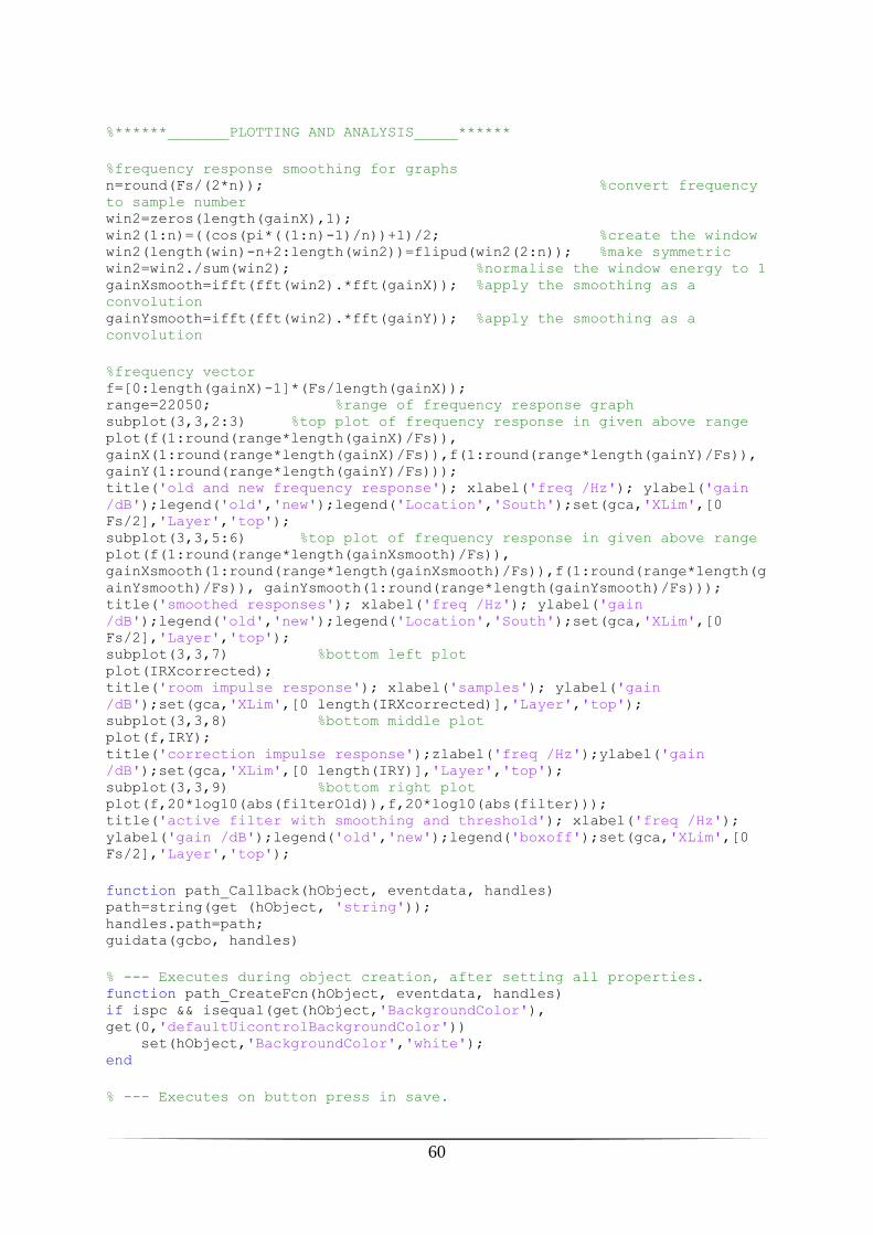
60
%******_______PLOTTING AND ANALYSIS_____******
%frequency response smoothing for graphs n=round(Fs/(2*n)); %convert frequency
to sample number win2=zeros(length(gainX),1); win2(1:n)=((cos(pi*((1:n)-1)/n))+1)/2; %create the window win2(length(win)-n+2:length(win2))=flipud(win2(2:n)); %make symmetric win2=win2./sum(win2); %normalise the window energy to 1 gainXsmooth=ifft(fft(win2).*fft(gainX)); %apply the smoothing as a
convolution gainYsmooth=ifft(fft(win2).*fft(gainY)); %apply the smoothing as a
convolution
%frequency vector f=[0:length(gainX)-1]*(Fs/length(gainX)); range=22050; %range of frequency response graph subplot(3,3,2:3) %top plot of frequency response in given above range plot(f(1:round(range*length(gainX)/Fs)),
gainX(1:round(range*length(gainX)/Fs)),f(1:round(range*length(gainY)/Fs)),
gainY(1:round(range*length(gainY)/Fs))); title('old and new frequency response'); xlabel('freq /Hz'); ylabel('gain
/dB');legend('old','new');legend('Location','South');set(gca,'XLim',[0
Fs/2],'Layer','top'); subplot(3,3,5:6) %top plot of frequency response in given above range plot(f(1:round(range*length(gainXsmooth)/Fs)),
gainXsmooth(1:round(range*length(gainXsmooth)/Fs)),f(1:round(range*length(g
ainYsmooth)/Fs)), gainYsmooth(1:round(range*length(gainYsmooth)/Fs))); title('smoothed responses'); xlabel('freq /Hz'); ylabel('gain
/dB');legend('old','new');legend('Location','South');set(gca,'XLim',[0
Fs/2],'Layer','top'); subplot(3,3,7) %bottom left plot plot(IRXcorrected); title('room impulse response'); xlabel('samples'); ylabel('gain
/dB');set(gca,'XLim',[0 length(IRXcorrected)],'Layer','top'); subplot(3,3,8) %bottom middle plot plot(f,IRY); title('correction impulse response');zlabel('freq /Hz');ylabel('gain
/dB');set(gca,'XLim',[0 length(IRY)],'Layer','top'); subplot(3,3,9) %bottom right plot plot(f,20*log10(abs(filterOld)),f,20*log10(abs(filter))); title('active filter with smoothing and threshold'); xlabel('freq /Hz');
ylabel('gain /dB');legend('old','new');legend('boxoff');set(gca,'XLim',[0
Fs/2],'Layer','top');
function path_Callback(hObject, eventdata, handles) path=string(get (hObject, 'string')); handles.path=path; guidata(gcbo, handles)
% --- Executes during object creation, after setting all properties. function path_CreateFcn(hObject, eventdata, handles) if ispc && isequal(get(hObject,'BackgroundColor'),
get(0,'defaultUicontrolBackgroundColor')) set(hObject,'BackgroundColor','white'); end
% --- Executes on button press in save.

61
function save_Callback(hObject, eventdata, handles) wavwrite(handles.IRY,handles.Fs,'correctionResponse.wav');
11.2 Amplitude Envelope Correction Code
clear all
Fs=44100; %sample rate f1=60; %start frequency f2=20000; %end frequency N=16; %order of the signal T=(2^N)/Fs; %length of the signal
% Create the swept sine tone w1=2*pi*f1; w2=2*pi*f2; K=T*w1/log(w2/w1); L=T/log(w2/w1); t=linspace(0,T-1/Fs,Fs*T)'; x1=sin(K*(exp(t/L) - 1)); x=[x1;x1]; %double the signal x=(1-(2/2^16))*x/max(max(abs(x))); %normalise
%play and record the sweep soundsc(x,Fs); X=wavrecord(length(x),Fs); %X=-1.*X; %phase reverse X=X((length(X)/2)+1:length(X)); %take second half of the recording X1=fft(X)./fft(x1); %deconvolution IRX=ifft(X1); X2=abs(X1); %absolute value X=(1-(2/2^16))*X/max(max(abs(X))); %normalise
%smoothing X ONLY first fifth of the spectrum n=10; %amount of smoothing win=zeros(round(length(X)/5),1); win(1:n)=((cos(pi*((1:n)-1)/n))+1)/2; %create the window win(length(win)-n+2:length(win))=flipud(win(2:n)); %make symmetric win=win./sum(win); %normalise the window energy to 1 X(1:round(length(X)/5))=ifft(fft(win).*fft(X(1:round(length(X)/5))));
%apply the smoothing as a convolution
%Find latency and compensate for it: impulse=max(max(abs(IRX(1:10000)))); for n=1:10000 if abs(IRX(n))==impulse latency=n; end end Xold=X; %for analysis X(1:end-latency+1)=X(latency:end);
%create arrays for negative crossover sample numbers ZeroVector=zeros(50,2); m=1; %initiate index for n=2:length(X)-1 if (x1(n+1)<0)&&(x1(n-1)>0) %if there is a zero crossing

62
ZeroVector(m,1)=n; m=m+1; %progress to next row end end m=1; %initiate index for n=2:length(X)-1 if (X(n+1)<0)&&(X(n-1)>0) %if there is a zero crossing ZeroVector(m,2)=n; m=m+1; %progress to next row end end
%calculate instantaneous wavelengths by number of samples between zero %crossings ZeroDiff=zeros(25,1); for n=2:25 ZeroDiff(n-1,1)=ZeroVector((2*n),1)-ZeroVector((2*n)-2,1); ZeroDiff(n-1,2)=ZeroVector((2*n),2)-ZeroVector((2*n)-2,2); end
ampEnv=zeros(length(X),1); %create amplitude
envolope cycles=0; %initiate number of
cycles for n=2:length(X)-1 if (X(n)>=X(n-1))&&(X(n)>=X(n+1))&&(X(n)>0) %find the local maxima
on positive peaks ampEnv(n)=X(n); %set data in sample
number to max amplitude cycles=cycles+1; %count the number of
cycles in the sweep end end
ampArray=zeros(cycles,2); %create array for
storing amplitude envelope data m=1; %initiate index for n=1:length(ampEnv) if ampEnv(n)>0 %ignore the zeros ampArray(m,1)=n; %set first column of the array to be sample number ampArray(m,2)=ampEnv(n); %set second column of the array to be the
amplitude m=m+1; %progress to the next
row of the array end end
%interpolation interpAmpEnv=ampEnv; %initiate interpolation
vector for n=1:ampArray(1,1)-1 interpAmpEnv(n)=n*ampArray(1,2)/ampArray(1,1); %interpolate up to the
first maximum end for m=1:cycles-1 for n=ampArray(m,1)+1:ampArray(m+1,1)-1 interpAmpEnv(n)=ampArray(m,2)+(n-ampArray(m,1))*(ampArray(m+1,2)-
ampArray(m,2))/(ampArray(m+1,1)-ampArray(m,1)); %interpolate between each
maximum end

63
end
%smoothing the interpolated envelope p=3; %amount of smoothing win2=zeros(length(interpAmpEnv),1); win2(1:p)=((cos(pi*((1:p)-1)/p))+1)/2; %create the window win2(length(win2)-p+2:length(win2))=flipud(win2(2:p)); %make symmetric win2=win2./sum(win2); %normalise the window energy to 1 smoothInterpAmpEnv=ifft(fft(win2).*fft(interpAmpEnv)); %apply the
smoothing as a convolution
%replace near-zeros with 0.01 to not divide by infinity for n=1:length(smoothInterpAmpEnv) if smoothInterpAmpEnv(n)<0.01 smoothInterpAmpEnv(n)=0.01; end end invAmpEnv=1./smoothInterpAmpEnv; invAmpEnv=abs(invAmpEnv);
%threshold on the inverted amplitude envelope thresh=7; %set threshold for anything above to be truncated invAmpEnv=invAmpEnv.*(invAmpEnv<thresh)+thresh*(invAmpEnv>thresh); %apply
threshold conserving phase data
y=x1.*invAmpEnv; %apply the envelope y1=[y;y]; %double the signal
%play and record the filtered sweep soundsc(y1,Fs); Y=wavrecord(length(y1),Fs); Y=Y((length(Y)/2)+1:length(Y)); %take second half Y1=fft(Y)./fft(x1); %deconvolution Y2=abs(Y1); %absolute value Y=(1-(2/2^16))*Y/max(max(abs(Y))); %normalise
%convert to dB gainY=20*log10(Y2); gainY=gainY-median(gainY); %centre around 0dB gainX=20*log10(X2); gainX=gainX-median(gainX); %centre around 0dB
%******_______PLOTTING AND ANALYSIS_____******
%frequency response smoothing for graphs m=500; %length of smoothing window win3=zeros(length(gainX),1); win3(1:m)=((cos(pi*((1:m)-1)/m))+1)/2; %create the window win3(length(win3)-m+2:length(win3))=flipud(win3(2:m)); %make symmetric win3=win3./sum(win3); %normalise the window energy to 1 gainXsmooth=ifft(fft(win3).*fft(gainX)); %apply the
smoothing as a convolution gainYsmooth=ifft(fft(win3).*fft(gainY)); %apply the
smoothing as a convolution
% frequency vector f=[0:length(gainX)-1]*(Fs/length(gainX)); range=22050; %range of frequency response graph subplot(2,1,1)

64
plot(f(1:round(range*length(gainXsmooth)/Fs)),
gainXsmooth(1:round(range*length(gainXsmooth)/Fs)),f(1:round(range*length(g
ainYsmooth)/Fs)), gainYsmooth(1:round(range*length(gainYsmooth)/Fs))); title('smoothed responses'); xlabel('freq /Hz'); ylabel('gain
/dB');legend('old','new');legend('Location','South');set(gca,'XLim',[0
Fs/2],'Layer','top');
%time vector time=1:length(X); subplot(2,1,2) plot(time,x1,time,X,time,smoothInterpAmpEnv,time,invAmpEnv,time,y) legend('original sweep','recorded sweep','recorded envelope','inverted
envelope','corrected sweep');legend('Location','EastOutside')
11.3 MLS Generation Code
clear all
Fs=44100; %sample rate
m=16; %order of the MLS to be calculated x=zeros((2^m)-1,1); %initiate length of MLS vector y=ones(m,1); %primitive poly for each time step N=length(x);
%create the MLS sequence for n=1:N x(n)= y(m); %MLS value set to the a(i) term of the poly %enter recursion relation for m... if m==1 z=rem(y(m),2); elseif m==2 z=rem(y(m)+y(m-1),2); elseif m==3 z=rem(y(m)+y(m-1),2); elseif m==4 z=rem(y(m)+y(m-1),2); elseif m==5 z=rem(y(m)+y(m-2),2); elseif m==6 z=rem(y(m)+y(m-1),2); elseif m==7 z=rem(y(m)+y(m-1),2); elseif m==8 z=rem(y(m)+y(m-6)+y(m-5)+y(m-1),2); elseif m==9 z=rem(y(m)+y(m-4),2); elseif m==10 z=rem(y(m)+y(m-3),2); elseif m==11 z=rem(y(m)+y(m-2),2); elseif m==12 z=rem(y(m)+y(m-7)+y(m-4)+y(m-3),2); elseif m==13 z=rem(y(m)+y(m-4)+y(m-3)+y(m-1),2);

65
elseif m==14 z=rem(y(m)+y(m-12)+y(m-11)+y(m-1),2); elseif m==15 z=rem(y(m)+y(m-1),2); elseif m==16 z=rem(y(m)+y(m-5)+y(m-3)+y(m-2),2); elseif m==17 z=rem(y(m)+y(m-3),2); elseif m==18 z=rem(y(m)+y(m-7),2); end y(2:m)=y(1:m-1); y(1)=z; end
%make sequence in terms of -1 and 1 for n=1:N if x(n)==0 x(n)=-1; end end
%play and record the sequence x=[x; x]; %double the length soundsc(x,Fs); %play the MLS Y=wavrecord(length(x),Fs); %record the MLS X=Y((length(Y)/2)+1:length(Y)); %take second half X=[X;0]; %correct the length X=(1-(2/2^16))*X/max(max(abs(X))); %normalise absX=abs(fft(X)); %take Fourier Transform
%convert to dB gain=20*log10(absX);
%frequency vector f=[0:length(gain)-1]*(Fs/length(gain)); subplot(2,1,1), semilogx(f(1:round(length(f)/2)),
gain(1:round(length(f)/2))); subplot(2,1,2), plot(f(1:round(400*length(gain)/Fs)),
gain(1:round(400*length(gain)/Fs)));