Long-Run Links AmongMoney, Prices, and Output:World-Wide Evidence

Helmut Herwartz(Humboldt-Universit�t zu Berlin)

Hans-Eggert Reimers(Hochschule Wismar)

Discussion paper 14/01

Economic Research Centre

of the Deutsche Bundesbank

September 2001

The discussion papers published in this series representthe authors’ personal opinions and do not necessarily reflect the viewsof the Deutsche Bundesbank.

Deutsche Bundesbank, Wilhelm-Epstein-Strasse 14, 60431 Frankfurt am Main,P.O.B. 10 06 02, 60006 Frankfurt am Main, Federal Republic of Germany

Telephone (0 69) 95 66-1Telex within Germany 4 1 227, telex from abroad 4 14 431, fax (0 69) 5 60 10 71Internet: http://www.bundesbank.de

Please address all orders in writing to: Deutsche Bundesbank,Press and Public Relations Division, at the above address, or by fax No. (0 69) 95 66-30 77

Reproduction permitted only if source is stated.

ISBN 3–933747–86–4

Abstract

Regarding inflation as being a monetary phenomenon in the long-run is a widely-held

view in modern macro economics. We analyse this topic by means of a P-star model.

Based on the quantity theory of money, this approach explains inflation via a supposed

equilibrium price level (P-star), which itself depends on potential output and money.

We investigate country-specific models for 110 economies, and also a pooled system

thereof. We test for cointegration among money, prices, and real output. Moreover,

parameter restrictions for the long-run relationships implied by the monetary theory

are tested. Country specific P-star variables are constructed and the cointegration

property between prices and the P-star variable is analysed. Along these lines, we find

that actual prices and their P-star counterparts are cointegrated at the pooled level

and thus demonstrate the importance of money for the development of prices.

Keywords: Quantity theory of money; Panel cointegration analysis;

Wild bootstrap inference.

JEL Classification: E31, C22

Zusammenfassung

Die Aussage, dass Inflation langfristig ein monetares Phanomen ist, ist eine grundle-

gende Erkenntnis der Makrookonomie. Dieser Sachverhalt wird in dieser Arbeit im

Rahmen eines P-Stern-Modells analysiert. Ausgehend von der Quantitatstheorie des

Geldes erklart der P-Stern-Ansatz die Inflationsrate mit Hilfe eines berechneten Gleich-

gewichtspreisniveaus (P-Stern), das vom Produktionspotential und von einer Geld-

menge abhangt. Wir untersuchen landerspezifische Modelle fur 110 Volkswirtschaften

und ein aus den Gleichungen bestehendes gepooltes System. Es wird auf Kointe-

gration zwischen einer Geldmenge, einem Preisniveau und dem realen Output testet.

Weiterhin werden die Parameterrestriktionen, die sich durch die monetare Theorie

ergeben, fur die langfristige Beziehung uberpruft. Zusatzlich werden nationale P-Stern-

Variablen konstruiert und es wird auf Kointegration zwischen diesen und den Preisen

getestet. Im empirischen Teil finden wir, wenn die Variablen gepoolt werden, dass die

aktuellen Preisniveaus mit den dazugehorenden P-Stern-Variablen kointegriert sind.

Dies verdeutlicht die Wichtigkeit des Geldes fur die Entwicklung der Preise.

Table of Contents

1 Introduction 1

2 The theoretical model 3

3 Methodology 6

4 Data and descriptive analysis 7

5 Econometric results 11

6 Conclusion 20

Appendix 21

References 23

List of Figures

Figure 1: Average yearly growth rates of M1, Mb, consumer price index and real

output for a maximal period from 1960 through 1999 for 110 countries 9

Figure 2: Box-Plots of estimated income elasticity 17

Figure 3: Recursive estimates of the adjustment coefficient and its p-value in the

inflation equation using M1 (Mb) where the countries arranged according

to their average inflation rate 19

List of Tables

Table 1: Regression results for the average inflation rate (real output

growth rate) and the growth rates of monetary aggregates 10

Table 2: Regression results for the United States 12

Table 3: Frequencies of rejection of cointegration and restriction hypotheses

for all countries 14

Table 4: Trimmed average estimates of the cointegration relationship 14

Table 5: Test results of the pooled ECM-equations 16

Table 6: Test results of H5 for the pooled P∗ equations 18

Long-Run Links Among Money, Prices, and Output:

World-Wide Evidence∗

1 Introduction

It is widely believed in modern macro economics that inflation is a monetary phe-

nomenon. Most central banks monitor monetary aggregates, and major central banks

are required to stabilize price movements. For instance, the European Central Bank

(ECB) has the primary objective of maintaining price stability in the Euro area (see

ECB, 1999). To stress the importance of monetary variables, the ECB gives one mon-

etary aggregate, namely M3, a prominent role in its strategy. An actual growth rate

of this aggregate, which exceeds its reference value is taken to indicate that the future

inflation rate may be higher than the target level.

The empirical evidence in favour of this inflation explanation is substantiated in two

ways. On the one hand, researchers are interested in stable money demand equations

for individual countries (e.g. see Lutkepohl & Wolters 1999). Given a stable equilib-

rium relation among output, prices, interest rates and money, monitoring the latter is

sensible when fighting inflation. Moreover, in such a situation it is feasible to control

money growth by means of interest rate adjustments. On the other hand, the long-

run relationship between money and prices is addressed in the so-called P-star model,

which is based on the quantity theory of money. It explains inflation via short-term

dynamic factors, and differences between the actual and an equilibrium price level,

which itself depends on money and potential output (Hallman et al. 1991, Todter &

∗Helmut Herwartz: Institute of Statistics and Econometrics, Humboldt–University Berlin, Span-

dauer Str. 1, D - 10178 Berlin, Germany, e-mail: helmut@wiwi.hu-berlin.de. Hans-Eggert Reimers,

Hochschule Wismar, University of Technique, Business and Design, Postfach 12 10, D - 23952 Wismar,

Germany, e-mail: h.reimers@wi.hs-wismar.de. Part of this research was conducted while the second

author was staying at the Deutsche Bundesbank as a visiting researcher. The hospitality of the Bun-

desbank is greatly appreciated. The paper was presented at seminars of the European Central Bank

and of the Economics Institute of the University of Regensburg. We thank the participants, especially

Heinz Herrmann and Franz Seitz, for their helpful comments. The views expressed in this study are

our own, and not those of the Deutsche Bundesbank.

1

Reimers 1994, Hoeller & Poret 1991, Kool & Tatom 1994, Gerlach & Svensson 2001).

Compared to a large body of econometric literature on money demand models,

only a few empirical studies focus directly on the link between prices and money.

Recently, McCandless & Weber (1995), Romer (1996) and Lucas (1996) have graph-

ically illustrated the comovement of money growth and inflation for more than 100

countries. Analysing a large set of macroeconomies the latter contributions are to be

recommended for the information base exploited. From an econometric point of view,

however, the approach adopted of unconditional empirical moments appears to be in-

efficient. It is more fruitful to take the dynamic structure of the involved variables into

account within a time series modelling framework.

Modern econometric concepts permit joint modelling of short and long-run dy-

namics, and therefore incorporate the ability of variables to adjust towards long-run

equilibrium. Especially if the variables are nonstationary, the concept of cointegration

is sensible (Engle & Granger 1987). Furthermore, to improve the power of common

test procedures in cointegrated systems it is sensible to enhance the information base

by pooling macroeconomic entities. Panel cointegration methods have attracted a lot

of interest in the recent econometric literature (Banerjee 1999). Pedroni (1997) pro-

poses a residual based procedure to test for cointegration in pooled dynamic systems.

Building on single equation error correction models Herwartz and Neumann (2000)

have introduced a bootstrap approach estimating critical values for common tests on

cointegration and equilibrium relations at the level of (high dimensional) pooled equa-

tions.

Extending the existing literature, we analyse the importance of money in the de-

velopment of prices where utilization of the panel approach is the main innovation.

Firstly, cointegration is tested among money, prices and real output for each coun-

try, and at the level of pooled economies. Secondly, restrictions of the cointegrating

space are tested for the pooled system. Thirdly, we construct country-specific P-star

variables, and, fourthly, test for cointegration between actual prices and the P-star

series. Following the P-star approach we find cointegration at the pooled level and

thus confirm the predominant role of money in the evolution of prices.

The remainder of the paper is organized as follows. In the next section the long-run

2

relation between money and prices is explained, and testable restrictions are given. In

Section 3 the bootstrap method adopted to obtain critical values for particular test

statistics is briefly provided. In Section 4 the data and descriptive analyses are given.

Section 5 presents empirical results. Section 6 summarizes and concludes.

2 The theoretical model

The long-run relation between money and prices is based on the quantity equation

P × Y = M × V, (1)

where P is the price level, Y is real output, M is the money supply and V is the

velocity of money. Owing to the definitions of the variables the relation in (1) is an

identity.

By making two simplifying assumptions, the quantity equation becomes a theory

of the cause of inflation. Firstly, the velocity of money is regarded as depending on the

institutional structure of the financial system that includes the payment system. Since

this system might be supposed to be time invariant, it is sensible to treat V as being

constant. If, secondly, output is exogenous for money, price changes in money must

be reflected in inflation rates. The practical relevance of the latter implication can be

illustrated by scatter plots showing average inflation rates against money supply growth

(Romer 1996, p. 392, McCandless and Weber 1995, p. 3). Moreover, McCandless and

Weber (1995) show that average money growth does not affect average output growth.

More recently, McCallum (2001) has emphasized that the unsystematic part of policy

instrument variability is small in relation to the variability of the systematic component.

Therefore, the investigation of the systematic component should dominate the analysis.

In a growing economy, Y may increase at some steady rate, thereby (partially)

”absorbing” money growth. Furthermore, invariance of the velocity of money is a

strong assumption, which should be confirmed. As long as output and velocity are in

equilibrium, however, equation (1) defines the equilibrium price level

P ∗ = (M/Y ∗)V ∗, (2)

where equilibrium values are indicated by a star (∗). P ∗ aims to measure the price

level to be obtained at the actual money holdings if production and velocity are in

3

equilibrium. If P and P ∗ are nonstationary and cointegrated, and the actual price level

is below its equilibrium, a future acceleration of inflation can be expected (Hallman et

al. 1991).

The equilibrium price level is not directly observable. To calculate P ∗, empirical

estimates of potential production and trend velocity are required. In some countries,

potential output is estimated, but it is not obvious how to obtain trend velocity. If log

velocity in time t (vt = lnVt) fluctuates randomly around a constant term, it becomes

vt = v0 + εt. If εt is a stationary zero mean process, the equilibrium level of log velocity

is v∗ = v0. In some countries, however, the velocities of monetary aggregates have

exhibited a marked downward trend in the past. Rather than assuming a deterministic

trend, Todter and Reimers (1994) propose incorporating a stochastic trend of velocity

if real money demand is income elastic (β1 > 1)

mt − pt = β0 + β1yt + zt, (3)

where yt is the log of real income (GDP), β0 is a constant term and β1 is the long-run

income elasticity of money demand. If zt is a stationary stochastic process with zero

mean, equation (3) describes a cointegration relationship. King and Watson (1997) re-

fer to (3) as being a monetary equilibrium condition. Contrary to this long-run relation,

a short-run dynamic money demand equation would have to take lagged adjustment

as well as interest rates into account.

Combining (1) and (3) yields the following expression for velocity

vt = −β0 + (1 − β1)yt − zt. (4)

This suggests measuring trend velocity as:

v∗t = −β0 + (1 − β1)y∗t

= v0 + (1 − β1)y∗t . (5)

For β1 = 1, this approach encompasses the stationary velocity case. If β1 > 1, a

declining trend of velocity is induced as long as potential output is growing.

Substituting (5) into the definition of P ∗ in (2), we end up with the following

measure of equilibrium prices:

p∗t = mt − β1y∗t + v0. (6)

4

Based on equation (15), there are some testable relationships. Firstly, one may be con-

cerned with cointegration between money, prices and real output, since these variables

are observable. The cointegrating relationship is written as

β2pt + β3mt + β1yt

and the first hypothesis we consider is:

H1 : pt, mt and yt are cointegrated.

Secondly, this long-run relation should not affect output, i.e.

H2 : output is weakly exogenous.

Thirdly, the coefficients of prices and money should be equal in absolute terms.

H3 : |β2| = |β3| price homogeneity or proportionality.

Fourthly, if the cointegration relation is normalized such that the coefficient of the price

level is unity, the coefficient of real output is (minus) unity:

H4 : |β1| = 1.

Condition H4 implies that the velocity of money is constant in the long run. If |β1| > 1,

it picks up a decreasing trend in velocity. If an estimate of potential output is available,

all these conditions are testable, applying a cointegration test between the equilibrium

price level and the actual price level. This test is based on an error correction model

for prices involving the price gap. Cointegration is found if the influence of the price

gap in the price equation is significant. Therefore, the final hypothesis we investigate

is

H5 : pt and p�t are cointegrated.

One further remark is make for H2. If output is weakly exogenous it is assumed that

y∗t is exogenous. The construction of v∗t via (5) implies that it is likewise exogenous.

5

3 Methodology

In this paper, we examine the monetary policy hypotheses given in the foregoing section

for a panel consisting of 110 economies. For this reason, we adopt a methodological

framework recently advocated by Herwartz and Neumann (2000), which is easily im-

plemented for large panels and allows asymptotically efficient inference even in the

presence of cross sectional error correlation. The method consists in aggregating OLS-

based single equation likelihood ratio (LR-) test statistics over the set of considered

economic entities. Both LR-tests on long-run parameters and on weak exogeneity

are aggregated without modelling contemporaneous error correlation explicitly. In the

presence of cross sectional error correlation, such a pooled LR-statistic is no longer

pivotal, and its asymptotic distribution depends on nuisance parameters. Herwartz

and Neumann (2000) prove the validity of a bootstrap procedure in estimating criti-

cal values for aggregated (dependent) LR-type statistics. As its main advantage the

methodology adopted here does not require any first step estimate of the underlying

pattern of contemporaneous error correlation. To account explicitly for cross sectional

error correlation in the present case considering 110 macroeconomies feasible gener-

alized least squares methods would require the estimation of a covariance matrix of

dimension 110 × 110.

In the following we provide only a brief account of the inference techniques adopted.

For a detailed discussion the reader is referred to Herwartz and Neumann (2000).

Assuming presample values to be available, we first consider the following single country

empirical model for real money (mrt):

∆mrt = δ0 + α1(pt−1 + β3mt−1 + β1yt−1) + δ1∆mrt−1

+δ2∆pt + δ3∆pt−1 + δ4∆yt + δ5∆yt−1 + ut. (7)

The adopted single equation approach to estimating long-run equilibrium relations is

asymptotically efficient if a set of assumptions can be made (Banerjee et al. 1993,

Chapter 6). In order to ensure the white noise property of ut, the equation in (7)

may be conveniently augmented by further (lagged) stationary explanatory variables.

The LR-statistics derived from the single equation ECM are typically represented as

T times the log ratio of the sum of residual squared errors, estimated via OLS under

6

a particular null hypothesis and its alternative, respectively. With RSS0 and RSS1

denoting these estimates the LR-statistic looks formally as follows:

LRn = T ln(RSS0

RSS1

). (8)

For some testing issues, it can be shown that LRn is asymptotically χ2(q) distributed,

with q denoting the number of excess parameters under the alternative model, com-

pared to the restricted model specified under the null hypothesis.

In Herwartz and Neumann (2000), it is shown that the so-called wild bootstrap

(Wu 1986) yields valid critical values if the LR-statistic is obtained from pooling over

a set of equations. To be more precise on the issue of pooling, consider now a set of

empirical error correction models, for example

∆mrnt = δn

0 + αn1 (p

nt−1 + βn

3mnt−1 + βn

1 ynt−1) + δn

1 ∆mrnt−1

+δn2∆p

nt + δn

3 ∆pnt−1 + δn

4 ∆ynt + +δn

5 ∆ynt−1 + un

t , n = 1, . . . , N, (9)

where N denotes the number of equations (countries) in the system. We are inter-

ested in testing a specific null hypothesis to hold in the pooled system. Assuming the

error terms of the N equations to be contemporaneously uncorrelated, a convenient

generalization of the statistic given in (8) is:

LRN =N∑

n=1

LRn = TN∑

n=1

ln(RSS0n

RSS1n

). (10)

In (10), we implicitly assume that T observations are available for each equation. Note

that LRN is easily modified if this assumption is violated. In the case of contemporane-

ous correlation between equations, critical values of the LRN -statistic can be obtained

by means of a bootstrap procedure. Apart from cross sectional correlation, the wild

bootstrap also accounts for heteroskedastic error distributions.

4 Data and descriptive analysis

The monetary policy hypotheses are examined for 110 countries. The data are from

the data base of the International Monetary Fund (international financial statistics).

To approximate price level and real output, we use the consumer price index (CPI)

and real gross domestic product (GDP), respectively. For some countries, the latter

7

variable is not available so that we replace it by nominal GDP deflated by CPI. As

the money variable, two alternatives are used. Firstly, we implement the empirical

analysis with a narrow definition of money, namely M1. Since notably central banks

of industrial countries stress the importance of a broad monetary aggregate, we also

used a variable Mb, which is defined as the sum of M1 and so-called quasi money. For

some members of the Eurozone, the latter variable cannot be constructed so that we

rely on a country-specific broad monetary aggregate (e.g. M3) to be found in the IMF

or Deutsche Bundesbank data base.

We investigate annual data for the (maximum) sample period 1960 to 1999. Mostly

data are available for (non-overlapping) country-specific subperiods, which cover at

least 15 years. All variables are measured in natural logarithms. Given alternative

definitions of money we analyse two sets of variables, namely

• S1: M1, CPI and real GDP, and

• S2: Mb, CPI and real GDP.

For Sweden and Italy, data on M1 and Mb are not available, respectively. Thus each

set used for the empirical analysis contains 109 countries.

To provide a first look at the data, we show average geometric growth rates of

real GDP, consumer prices and the two definitions of money. In the upper panels of

Figure 1 scatter plots are given for growth of M1 and Mb versus CPI inflation. To

facilitate their interpretation both illustrations also show the 45◦-line. Observations

for individual countries are close to the diagonal. This result does not depend on the

definition of money employed and is confirmed by regressing the average inflation rate

on a constant and money growth. Results for such a regression are shown in Table

1. The degree of explanation (R2) is rather high, and the coefficients of the money

variables are close to unity. These results are in line with evidence in de Grauwe and

Grimaldi (2001).

8

Figure 1: Average yearly growth rates of M1, Mb, consumer price index and real output

for a maximal period from 1960 through 1999 for 110 countries.

Considering two subsets, namely the set of countries belonging for more than 10

years to the OECD† and the set of Latin America economies,‡ it is worth emphasizing

that there are only small regional differences. Similar charts covering the 1960-90 pe-

†The set OECD includes the countries: Austria, Australia, Belgium, Canada, Denmark, Finland,

France, Germany, Greece, Iceland, Italy, Ireland, Japan, Netherlands, New Zealand, Norway, Portugal,

Spain, Switzerland, Turkey, United Kingdom, and United States.‡Latin America comprises Argentina, Bahamas, Bolivia, Brazil, Chile, Colombia, Costa Rica,

Dominican Republic, El Salvador, Guatamala, Haiti, Honduras, Jamaica, Mexico, Panama, Paraquay,

Peru, Uruguay, Venezuela.

9

riod can be found in McCandless and Weber (1995). Brazil has the highest inflation

rate and money growth rate. Both plots and the regression results seem to confirm

a one-to-one relationship between money growth and inflation. Moreover, de Grauwe

and Grimaldi (2001) analyse the stability of the money coefficient as a function of the

level of inflation. The data are arranged in ascending and descending order of inflation.

They show that the money coefficient increases with the average inflation rate. For

low inflation countries, the coefficients are not significantly different from zero. Adding

high inflation countries to the sample leads to an increasing coefficient. Including all

countries, the latter coefficient is close to unity.

Table 1: Regression results for the average inflation rate (real output growth rate)

and the growth rates of monetary aggregates.

Vari- Regions

ables All countries OECD Latin America

∆p C ∆m1 R2 C ∆m1 R2 C ∆m1 R2

−4.25(13.25)

1.04(78.01)

0.983 −2.46(3.59)

0.94(17.14)

0.936 −4.21(6.14)

1.04(66.97)

0.996

∆p C ∆mb R2 C ∆mb R2 C ∆mb R2

−5.29(13.31)

1.00(64.95)

0.975 −2.84(5.92)

0.87(24.74)

0.968 −5.69(7.06)

1.00(58.26)

0.995

∆y C ∆m1 R2 C ∆m1 R2 C ∆m1 R2

4.03(13.69)

−0.011(0.86)

0.006 3.10(8.49)

0.038(1.35)

0.083 3.22(6.53)

0.013(0.97)

0.051

∆y C ∆mb R2 C ∆mb R2 C ∆mb R2

3.95(12.86)

−0.006(0.49)

0.002 3.02(8.50)

0.036(1.48)

0.099 3.20(6.25)

0.012(0.98)

0.050

Maximum of information period: 1960-1999. Estimated t-values in parentheses. OECD

includes countries that have been members of the organization for more than ten years.

The lower panels of Figure 1 show average growth rates of money versus real output

for all the countries considered. The overall average growth rate of real output is also

displayed. It appears that money growth does not affect the growth of real output.

Moreover, output growth is regressed on an intercept and money growth. Regression

results are also given in Table 1. Regardless of the monetary aggregate employed its

coefficient is not significantly different from zero in a regression covering all countries.

10

The degree of explanation is small. The latter findings are in line with McCandless

and Weber (1995), as well as de Grauwe and Grimaldi (2001). Performing the latter

regression for the OECD subset, we find that the coefficient of growth of the broad

monetary aggregate is positive and the corresponding t-value and R2 are higher com-

pared with the remaining cases considered. On the one hand, this result may indicate

that, for the industrial countries, money may lose its neutrality. On the other hand,

however, the interpretation could be reversed, i.e. the money supply is extended if the

growth rate of a country increases.

5 Econometric results

Neglecting the time series dimension of the data, the comparison of average growth

rates, as adopted so far, is a weak econometric concept in terms of efficiency. In the

following single equation error correction models (ECMs) are used to reexamine long-

run links between prices and money as well as money and real output. Its application

requires the variables to be integrated of order one and one cointegrating relationship

to exist among the variables. These assumptions are tested via the multivariate maxi-

mum likelihood methodology (Johansen 1995), which yields evidence of more than one

cointegration relation for only 17 countries.§ For each set of variables, we specify three

country-specific ECMs, namely:

∆mrt = ν1 + α1(pt−1 + β3mt−1 + β1yt−1) + r1t + u1t, (11)

∆yt = ν2 + α2(pt−1 + β3mt−1 + β1yt−1) + r2t + u2t, (12)

∆pt = ν3 + α3(pt−1 + β3mt−1 + β1yt−1) + r3t + u3t. (13)

The processes rit, i = 1, 2, 3 in (11) to (13) are equation-specific linear combinations of

stationary variables (current and lagged values of ∆mrt, ∆mt, ∆yt, ∆pt), the inclusion

of which turned out to be necessary so as to yield serially uncorrelated error terms uit.

Since the particular composition of rit varies across countries and is informative only

for short-run dynamics, we employ this brief notation. Within the empirical exercises,

we aim to specify rit as parsimoniously as possible. In fact, each estimated coefficient

in rit has an absolute t−ratio of at least 1.5.

§The results are available from the authors upon request.

11

Table 2: Regression results for the United States

Regres.- Dependent variables

sors ∆m1r ∆mbr ∆y ∆y ∆p ∆p

C −0.058(0.44)

0.022(0.12)

0.163(1.76)

0.142(1.62)

−0.149(2.62)

−0.083(1.30)

m1t−1 −1.651(7.69)

−1.139(1.62)

−0.817(2.84)

mbt−1 −0.767(5.98)

6.647(0.11)

0.327(1.24)

pt−1 0.286(4.88)

0.295(3.76)

0.050(1.13)

−0.004(0.10)

−0.093(3.03)

−0.065(2.12)

yt−1 1.628(3.75)

0.330(0.93)

0.282(0.19)

16.92(0.10)

−0.040(0.07)

−0.686(1.02)

∆m1rt−1 0.384(3.45)

∆mbrt−1 0.687(4.39)

∆p −1.393(6.84)

∆pt−1 0.512(2.02)

−0.517(3.70)

−0.470(4.88)

1.075(8.92)

0.958(9.92)

∆yt−1 0.458(3.79)

0.372(3.18)

∆yt−2 −0.215(1.51)

∆m1t−1 0.100(1.79)

∆mb −0.114(1.91)

∆mbt−1 0.191(2.62)

R2 0.71 0.57 0.43 0.53 0.85 0.84

DW 1.97 1.74 2.18 2.21 1.82 1.70

Estimated subset models in the error correction form for the United States. Informa-

tion period: 1960-1999. Estimated t-values in parentheses.

The two sets of variables differ with respect to the monetary aggregate employed,

i.e. the variable mt is either narrowly (mt = m1t) or broadly (mt = mbt) defined.

The coefficients αi, i = 1, 2, 3, indicate how the dependent variable responds to lagged

violations of the long-run equilibrium relation, and it is expected to be negative (posi-

tive) for the first (third) equation. If output is weakly exogenous for inference on the

12

long-run equilibrium, α2 is expected to be zero (H2). In some cases, the empirical mod-

els are augmented with one or two impulse dummy variables to account for ‘extreme’

outliers. The overall performance of the specification strategy adopted is monitored by

means of the Durbin-Watson (DW) and the Box-Pierce statistic (of order 4 or 8), which

we regard as a convenient descriptive statistic for empirical models containing lagged

dependent variables. For almost all of the 654 regression models the DW-statistic is

close to 2, indicating convenient selections of lagged stationary regressor variables in

(11) to (13).

The selected (subset) single equation models are used to implement LR-tests on the

level of pooled equations. To provide a particular example for the empirical analysis

the results for the US are given in Table 2. The cointegration hypothesis is tested

using the t-value of the loading coefficient (H1 : α1 = 0). In the price equation, it

is the coefficient of the lagged price variable. Its t-value is 3.03, which is significant

at the 5% level. Weak exogeneity of variables implies that the specified cointegration

relationship is not significant in the other equations. Thus the loading coefficient of

the cointegration relation should be zero in the output equation (H2 : α2 = 0). The

estimated t-value is 1.13. The hypothesis of weak exogeneity cannot be rejected. For

the price homogeneity hypothesis, the coefficient of the money level in price equation

should be unity in absolute terms (H3). Its estimated absolute value is 0.817, which is

supposed not to differ significantly from unity. The unrestricted estimate of β1 is .04:

hypothesis H4 is rejected.

The described tests are conducted for each country. Rejection frequencies for the

particular hypotheses are given in Table 3. Three significance levels are distinguished.

Alternatively, critical values are taken from the χ2-distribution and estimated via a

bootstrap approach. Given that the former method turned out to be severely oversized

for typical sample sizes, it is not surprising that the bootstrap procedure yields rejec-

tions of all null hypotheses less frequently. Using critical values from the bootstrap,

the hypothesis of no cointegration is rejected for 57 countries at the 5% test level.

13

Table 3: Frequencies of rejection of cointegration and restriction hypotheses for all

countries.

Asymptotic Bootstrapped

critical values critical values

Equation Hypothesis 0.01 0.05 0.10 0.01 0.05 0.10

Set 1 ∆m1r H1 : coint. 52 70 77 21 57 68

H3 : |β3| = 1 35 46 55 18 36 43

Set 2 ∆mbr H1: coint. 38 62 71 15 42 61

H3 : |β3| = 1 26 38 44 13 26 36

Set 1 ∆y H2: exog. 19 37 47 7 22 37

Set 2 ∆y H2: exog. 18 31 42 10 23 33

Set 1 ∆p H1: coint. 38 56 62 19 43 55

Set 2 ∆p H1: coint. 32 50 64 11 38 53

Maximum of information period: 1960-1999. Number of countries: 109. Set 1 (2)

includes M1, Y and P (Mb, Y and P), respectively. Hypothesis ’coint’: null hypothesis

of no cointegration is tested in the corresponding equation. The test uses the loading

coefficient to check the hypothesis. Hypothesis ’exog’: null hypothesis of weakly exoge-

nous variable for the cointegration relationship. The assumed p-values, depending on

the asymptotic results (bootstrapped approach), for the critical values are 0.01, 0.05

and 0.10.

Table 4: Trimmed average estimates of the cointegration relationship:

αi(pt−1 + β3mt−1 + β1yt−1)

Set 1 Set 2

Equation pt−1 m1t−1 yt−1 pt−1 mbt−1 yt−1

∆mr 0.462 -1.067 1.053 0.314 -0.857 0.614

∆y -0.243 -0.746 0.465 -0.267 -1.120 2.319

∆p -0.101 -0.679 -0.460 -0.092 -0.763 0.697

Maximum of information period: 1960-1999. Number of countries: 109. Set 1 (2)

includes M1, P and Y (Mb, P and Y), respectively.

To give an impression of the coefficient estimates obtained trimmed average values

are shown in Table 4. To mitigate the impact of outlying estimates on these averages,

the two biggest and two smallest coefficient estimates do not contribute to the reported

14

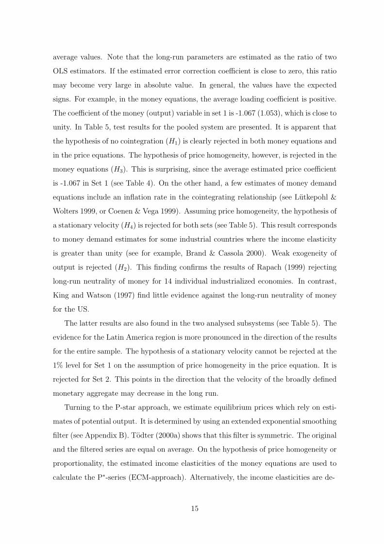
average values. Note that the long-run parameters are estimated as the ratio of two

OLS estimators. If the estimated error correction coefficient is close to zero, this ratio

may become very large in absolute value. In general, the values have the expected

signs. For example, in the money equations, the average loading coefficient is positive.

The coefficient of the money (output) variable in set 1 is -1.067 (1.053), which is close to

unity. In Table 5, test results for the pooled system are presented. It is apparent that

the hypothesis of no cointegration (H1) is clearly rejected in both money equations and

in the price equations. The hypothesis of price homogeneity, however, is rejected in the

money equations (H3). This is surprising, since the average estimated price coefficient

is -1.067 in Set 1 (see Table 4). On the other hand, a few estimates of money demand

equations include an inflation rate in the cointegrating relationship (see Lutkepohl &

Wolters 1999, or Coenen & Vega 1999). Assuming price homogeneity, the hypothesis of

a stationary velocity (H4) is rejected for both sets (see Table 5). This result corresponds

to money demand estimates for some industrial countries where the income elasticity

is greater than unity (see for example, Brand & Cassola 2000). Weak exogeneity of

output is rejected (H2). This finding confirms the results of Rapach (1999) rejecting

long-run neutrality of money for 14 individual industrialized economies. In contrast,

King and Watson (1997) find little evidence against the long-run neutrality of money

for the US.

The latter results are also found in the two analysed subsystems (see Table 5). The

evidence for the Latin America region is more pronounced in the direction of the results

for the entire sample. The hypothesis of a stationary velocity cannot be rejected at the

1% level for Set 1 on the assumption of price homogeneity in the price equation. It is

rejected for Set 2. This points in the direction that the velocity of the broadly defined

monetary aggregate may decrease in the long run.

Turning to the P-star approach, we estimate equilibrium prices which rely on esti-

mates of potential output. It is determined by using an extended exponential smoothing

filter (see Appendix B). Todter (2000a) shows that this filter is symmetric. The original

and the filtered series are equal on average. On the hypothesis of price homogeneity or

proportionality, the estimated income elasticities of the money equations are used to

calculate the P∗-series (ECM-approach). Alternatively, the income elasticities are de-

15

Table 5: Test results of the pooled ECM-equations.

Equa- Hypo- Set 1 Set 2

Region tion thesis test value p-value test value p-value

World ∆mr H1 : coint. 581.40 0.000 420.48 0.000

H3 : |β3| = 1 1033.36 0.000 857.55 0.000

∆y H2 : exog. 497.61 0.000 509.07 0.000

∆p H1 : coint. 745.68 0.000 680.10 0.000

H3 : |β3| = 1 1296.58 0.000 1195.39 0.000

H4 : |β1| = 1||β3| = 1 751.46 0.000 564.67 0.000

Latin ∆mr H1 : coint. 135.88 0.000 111.38 0.000

America H3 : |β3| = 1 193.35 0.000 189.92 0.000

∆y H2 : exog. 91.68 0.000 67.97 0.002

∆p H1 : coint. 136.52 0.000 91.68 0.000

H3 : |β3| = 1 188.18 0.000 163.77 0.000

H4 : |β1| = 1||β3| = 1 192.46 0.000 141.21 0.000

OECD ∆mr H1 : coint. 143.41 0.000 84.05 0.000

H3 : |β3| = 1 277.21 0.000 134.90 0.000

∆y H2 : exog. 64.60 0.002 63.94 0.000

∆p H1 : coint. 169.23 0.000 141.03 0.000

H3 : |β3| = 1 267.91 0.000 262.84 0.000

H4 : |β1| = 1||β3| = 1 52.16 0.017 60.41 0.001

Maximum of information period: 1960-1999. Number of countries: 109. Set 1 (2)

includes M1, P and Y (Mb, P and Y), respectively. The p-values are calculated by the

bootstrap approach.

termined by the static Engle-Granger cointegration regression (Engle and Granger

1987):

mt − pt = c0 + β1yt + zt, (14)

where zt is a stationary process. The estimated coefficient β1 is used to calculate the

P∗-series. The specification of the dynamic price equation is:

∆pt = δ0 + α4(pt−1 − p∗t−1) + δ1∆pt−1 + δ2∆pt−2 + δ3∆p∗t + u4t. (15)

where u4t is a white noise process. Equation (15) includes the price gap (pt−1 − p∗t−1)

and dynamic factors. In contrast to Gerlach and Svensson (2001), who use quarterly

16

observations on ∆p∗t−1, we employ annual data. The model (15) allows us to test the

hypothesis:

H5 : α4 = 0 .

Figure 2 gives the Box-plots of estimated income coefficient (β1). It is seen that the

ECM-approach yields more extreme values of β1 compared with the static regression

(14).

Income elasticity from cointegrating relationship

M1 Mb M1 (E-G) Mb (E-G)

Figure 2: Box-Plots of estimated income elasticity β1 of the restricted cointegration

relationship (m + p + β1y) or of Engle-Granger cointegration relation. Upper bound

(lower bound) corresponds to the 95th (5th) quantil.

17

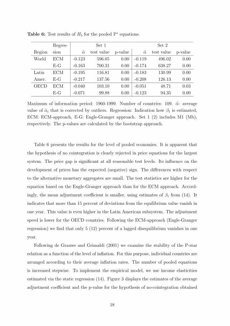
Table 6: Test results of H5 for the pooled P∗ equations.

Regres- Set 1 Set 2

Region sion α test value p-value α test value p-value

World ECM -0.123 596.05 0.00 -0.119 496.02 0.00

E-G -0.163 700.31 0.00 -0.174 638.27 0.00

Latin ECM -0.195 116.81 0.00 -0.183 130.99 0.00

Amer. E-G -0.217 137.56 0.00 -0.208 126.13 0.00

OECD ECM -0.040 103.10 0.00 -0.051 48.71 0.03

E-G -0.071 99.88 0.00 -0.123 94.35 0.00

Maximum of information period: 1960-1999. Number of countries: 109. α: average

value of αi that is corrected by outliers. Regression: Indication how β1 is estimated,

ECM: ECM-approach, E-G: Engle-Granger approach. Set 1 (2) includes M1 (Mb),

respectively. The p-values are calculated by the bootstrap approach.

Table 6 presents the results for the level of pooled economies. It is apparent that

the hypothesis of no cointegration is clearly rejected in price equations for the largest

system. The price gap is significant at all reasonable test levels. Its influence on the

development of prices has the expected (negative) sign. The differences with respect

to the alternative monetary aggregates are small. The test statistics are higher for the

equation based on the Engle-Granger approach than for the ECM approach. Accord-

ingly, the mean adjustment coefficient is smaller, using estimates of β1 from (14). It

indicates that more than 15 percent of deviations from the equilibrium value vanish in

one year. This value is even higher in the Latin American subsystem. The adjustment

speed is lower for the OECD countries. Following the ECM-approach (Engle-Granger

regression) we find that only 5 (12) percent of a lagged disequilibrium vanishes in one

year.

Following de Grauwe and Grimaldi (2001) we examine the stability of the P-star

relation as a function of the level of inflation. For this purpose, individual countries are

arranged according to their average inflation rates. The number of pooled equations

is increased stepwise. To implement the empirical model, we use income elasticities

estimated via the static regression (14). Figure 3 displays the estimates of the average

adjustment coefficient and the p-value for the hypothesis of no-cointegration obtained

18

P-star using M1 P-star using Mb

Figure 3: Recursive estimates of the adjustment coefficient and its p-value in the infla-

tion equation using M1 (Mb) where the countries arranged according to their average

inflation rate.

from the bootstrap. Apparently, the absolute adjustment coefficient increases if coun-

tries with higher inflation are added to the sample. It takes more time in low inflation

countries to obtain the long-run relation than in high inflation countries. If the equi-

librium price level constructed with Mb is considered, we find that the cointegrating

relationship is not significant in countries having very low inflation rates (see the lower

right-hand panel of Figure 3). This finding changes if the equilibrium price level cal-

culated by M1 is considered where the cointegrating relationship is also significant in

low inflation countries (see the lower left-hand panel of Figure 3). This result indicates

19

that the proportionality between money and prices also appears under these economic

conditions. Note that proportionality is reflected by variables measured in levels. By

merely relying on (average) growth rates, such a relationship cannot be uncovered.

6 Conclusion

Using the P-star model framework, which bases on the quantity theory of money and

allows us to estimate a nonstationary velocity of money, we analyse the development

of prices in 110 macroeconomies. Using annual data, the observation period is, at

most, 1960 through 1999. To improve the power of the tests, a panel cointegration

approach is used. From a methodological point of view, the analysis permits us to

consider economic relationships for variables in levels, rather than relying on descriptive

comparisons of average growth rates. Critical values for LR-tests are determined by

means of a bootstrap procedure.

At the pooled level, we find evidence of cointegration relating actual prices and an

equilibrium price level termed P-star. It is found for the entire sample, as well as for

two subsets, the OECD and Latin America. The long-run link is obtained for high

inflation countries and, in general, for low inflation countries. With respect to mone-

tary policy, our results underscore that it is necessary for central banks to monitor the

development of monetary aggregates. Monetary aggregates determine the price level

in the long run, and the control of its development is a cornerstone for achieving price

stability in the long run.

20

Appendix A: The countries analysed:

Algeria, Argentina, Australia, Austria, Bahamas, Bahrain, Bangladesh, Belgium, Be-

lize, Bhutan, Bolivia, Botswana, Brazil, Burkina Faso, Burundi, Cameroon, Canada,

Central African Republic, Chad, Chile, Colombia, Congo (Democratic Republic of),

Congo (Republic of), Costa Rica, Cote d Ivoire, Cyprus, Denmark, Dominica, Domini-

can Republic, Ecuador, Egypt, El Salvador, Ethiopia, Fiji, Finland, France, Gabon,

Gambia, Germany, Greece, Guatemala, Haiti, Honduras, Hungary, Iceland, India, In-

donesia, Iran, Ireland, Israel, Italy, Jamaica, Japan, Jordan, Kenya, Korea, Kuwait,

Lesotho, Madagascar, Malawi, Malaysia, Mauritania, Mexico, Morocco, Nepal, Nether-

lands, New Zealand, Nicaragua, Niger, Nigeria, Norway, Pakistan, Panama, Paraguay,

Peru, Philippines, Portugal, Qatar, Rwanda, Samoa, Saudi Arabia, Senegal, Seychelles,

Sierra Leone, Singapore, South Africa, Spain, Sri Lanka, Sudan, Swaziland, Sweden,

Switzerland, Syria, St. Kitts-Nevis, St. Lucia, St. Vincent, Tanzania, Thailand, Togo,

Tonga, Trinidad, Tunisia, Turkey, United Arab Emirates, United Kingdom, United

States, Uruguay, Venezuela, Zambia, Zimbabwe.

Appendix B: Estimation of Potential Output

The estimation of potential output Y ∗ is conducted by a statistical procedure. Follow-

ing Todter (2000a), the procedure is derived from the function:

Z := Min

(yt,c1)

(λ

2

T∑t=2

(yt − yt−1 − c1)2 +

1 − λ

2

T∑t=1

(yt − yt)2)

The first term reflects the smoothness of the filtered series, and the second term gives

the adjustment of the estimated series on the observed series. The first-order conditions

are determined by differencing the function to all yt and c1. The conditions imply that

the intercept term c1 may be determined by the following nonparametric estimate:

c1 =1

T − 1

T∑t=2

(yt − yt−1) =yT − y1

T − 1

21

The filtered series is:

Y ∗ = A−1Y

where

A = 11−λ

1 − λT−1

−λ 0 0 · · · λT−1

−λ 1 + λ −λ 0 · · · 0

0 −λ 1 + λ −λ · · · 0...

. . . . . ....

0 1 + λ −λ 0

0 −λ 1 + λ −λλ

T−10 · · · 0 −λ 1 − λ

T−1

The filter, which is denoted as extended exponential smoothing, is:

Y ∗t =

2λ

1 + λ

(Y ∗

t−1 + Y ∗t+1

2

)+

1 − λ

1 + λYt

for t = 1, · · · , T − 1 and λ = 1+θ2

, where θ is the first-order autocorrelation coefficient

of the variable wt

Yt = Yt−1 + c1 + wt

The series wt is the OLS-residuals of this equation. Hence, this implies another ap-

proach to estimate c1 (see Todter, 2000b). This equation allows us to account for

impulse dummies at a known break point. If a series includes an impulse dummy, the

filtering step is adjusted. First, the series is corrected by the impulse dummy. Second,

the filtered series is determined. Third, the effect of the impulse dummy is added to

the filtered series.¶

¶The countries including an impulse dummy are Argentina, Belgium, Gabon, Germany, Lesotho,

Netherlands, Samoa, Sri Lanka and Tanzania.

22

References

Banerjee, A. (1999): Panel Data Unit Roots and Cointegration: An Overview, Oxford

Bulletin of Economics and Statistics, vol. 61, pp. 607–629.

Banerjee, A., J. Dolado, J.W. Galbraith, D.F. Hendry (1993): Co-Integration, Error-

Correction, and the Econometric Analysis of Non-Stationary Data, Oxford Uni-

versity Press, Oxford.

Brand, C., N. Cassola (2000): A Money Demand System for Euro Area M3, Working

Paper No. 39, European Central Bank, Frankfurt am Main.

Bullard, J. (1999): Testing Long-Run Monetary Neutrality Propositions: Lessons

from the Recent Research, Review of the Federal Reserve Bank of St. Louis, vol.

61, no. 6, pp. 57–77.

Coenen, G., J.-L. Vega (1999): The Demand for M3 in the Euro Area, Working Paper

No. 6, European Central Bank, Frankfurt am Main.

De Grauwe, P., M. Grimaldi (2001): Exchange Rates, Prices and Money: A Long Run

Perspective, Discussion paper, University of Leuven.

European Central Bank (1999): The Stability-oriented Monetary Policy Strategy of

the Eurosystem, Monthly Report, vol. 1, January, p. 39–50.

Gerlach, S., L.E.O. Svensson (2001): Money and Inflation in the Euro Area: A Case

for Monetary Indicators?, Working Papers No. 98, Monetary and Economic

Department, Bank for International Settlements, Basle.

Hallman, J.J., R.D. Porter, D.H. Small (1991): Is the Price Level Tied to the M2

Monetary Aggregates in the Long Run?, The American Economic Review, 81,

841–858.

Herwartz, H., M.H. Neumann (2000): Bootstrap Inference in Single Equation Error

Correction Models, Discussion paper no. 87, Humboldt-University Berlin.

Hoeller, P., P. Poret (1991): Is P-star a Good Indicator of Inflationary Pressure in

OECD Countries?, OECD Economic Studies, no. 17.

23

Johansen, S. (1995): Likelihood-based Inference in Cointegrated Vector Autoregressive

Models, Oxford University Press, Oxford.

King, R.G., M.W. Watson (1997): Testing Long-Run Neutrality, Economic Quarterly,

Federal Reserve Bank of Richmond, vol. 83 (Summer), pp. 69–101.

Kool, C.J., J.A. Tatom (1994): The P-star Model in Five Small Economies, Review

of the Federal Reserve Bank of St. Louis, vol. 76, no. 3, p. 11–29.

Lucas, R.E. (1996): Nobel Lecture: Monetary Neutrality, Journal of Political Econ-

omy, vol. 104, pp. 661-682.

Lutkepohl, H., J. Wolters (eds.) (1999): Money demand in Europe, Physica Verlag,

Heidelberg.

McCallum, T. (2001): Analysis of the Monetary Transmission Mechanism: Method-

ological Issues, in: Deutsche Bundesbank (ed.) The Monetary Transmission Pro-

cess, Recent Develoment and Lessons for Europe, p. 11–43, Palgrave, Houndmills.

McCandless, G.T., W.E. Weber (1995): Some Monetary Facts, Federal Reserve Bank

of Minneapolis, Quarterly Review, Summer, 19, 2-11.

Orphanides, A., R. Porter (1998): P∗ Revisited: Money-Based Inflation Forecasts

with a Changing Equilibrium Velocity, Discussion paper, Board of Governors of

the Federal Reserve System, Washington.

Pedroni, P. (1997): Panel Cointegration: Asymptotic and Finite Sample Properties

of Polled Time Series Tests with an Application to the PPP Hypothesis, New

Results, Indiana University Working Paper in Economics.

Rapach, D.E. (1999): International Evidence on the Long-Run Superneutrality of

Money, Discussion paper, Trinity College, Washington.

Romer, D. (1996) Advanced Macroeconomics, McGraw-Hill, New York.

Todter, K.-H. (2000a): Erweiterte exponentielle Glattung als Instrument der Zeitrei-

henanalyse, I. Eine Alternative zum Hodrick-Prescott-Filter, Deutsche Bundes-

bank, mimeo.

24

Todter, K.-H. (2000b): Erweiterte exponentielle Glattung als Instrument der Zeitrei-

henanalyse, II. Zur Wahl des Glattungsparameters, Deutsche Bundesbank, mimeo.

Todter, K.-.H, H.-E. Reimers (1994): P -Star as a Link Between Money and Prices in

Germany, Weltwirtschaftliches Archiv, 130, 273–289.

Wu, C.F.J. (1986). Jackknife, Bootstrap, and Other Resampling Methods in Regres-

sion Analysis (with discussion), Annals of Statistics, 14, 1261–1295.

25

26

The following papers have been published since 2000:

February 2000 How Safe Was the „Safe Haven“?Financial Market Liquidity duringthe 1998 Turbulences Christian Upper

May 2000 The determinants of the euro-dollarexchange rate – Synthetic fundamentals Jörg Clostermannand a non-existing currency Bernd Schnatz

July 2000 Concepts to Calculate EquilibriumExchange Rates: An Overview Ronald MacDonald

August 2000 Kerinflationsraten: Ein Methoden-vergleich auf der Basis westdeutscherDaten * Bettina Landau

September 2000 Exploring the Role of Uncertaintyfor Corporate Investment Decisionsin Germany Ulf von Kalckreuth

November 2000 Central Bank Accountability andTransparency: Theory and Some Sylvester C.W. EijffingerEvidence Marco M. Hoeberichts

November 2000 Welfare Effects of Public Stephen MorrisInformation Hyung Song Shin

November 2000 Monetary Policy Transparency, PublicCommentary, and Market Perceptionsabout Monetary Policy in Canada Pierre L. Siklos

* Available in German only.

27

November 2000 The Relationship between the FederalFunds Rate and the Fed’s Funds RateTarget: Is it Open Market or OpenMouth Operations? Daniel L. Thornton

November 2000 Expectations and the Stability Problem George W. Evansfor Optimal Monetary Policies Seppo Honkapohja

January 2001 Unemployment, Factor Substitution, Leo Kaasand Capital Formation Leopold von Thadden

January 2001 Should the Individual Voting Records Hans Gersbachof Central Banks be Published? Volker Hahn

January 2001 Voting Transparency and Conflicting Hans GersbachInterests in Central Bank Councils Volker Hahn

January 2001 Optimal Degrees of Transparency inMonetary Policymaking Henrik Jensen

January 2001 Are Contemporary Central BanksTransparent about Economic Modelsand Objectives and What DifferenceDoes it Make? Alex Cukierman

February 2001 What can we learn about monetary policy Andrew Claretransparency from financial market data? Roger Courtenay

March 2001 Budgetary Policy and Unemployment Leo KaasDynamics Leopold von Thadden

March 2001 Investment Behaviour of German EquityFund Managers – An Exploratory Analysisof Survey Data Torsten Arnswald

28

April 2001 Der Informationsgehalt von Umfrage-daten zur erwarteten Preisentwicklungfür die Geldpolitik * Christina Gerberding

May 2001 Exchange rate pass-throughand real exchange ratein EU candidate countries Zsolt Darvas

July 2001 Interbank lending and monetary policy Michael EhrmannTransmission: evidence for Germany Andreas Worms

September 2001 Precommitment, Transparency and Montetary Policy Petra Geraats

September 2001 Ein disaggregierter Ansatz zur Berechnungkonjunkturbereinigter Budgetsalden fürDeutschland: Methoden und Ergebnisse * Matthias Mohr

September 2001 Long-Run Links Among Money, Prices, Helmut Herwartzand Output: World-Wide Evidence Hans-Eggert Reimers

* Available in German only.

29

Visiting researcher at the Deutsche Bundesbank

The Deutsche Bundesbank in Frankfurt is looking for a visiting researcher. Visitors shouldprepare a research project during their stay at the Bundesbank. Candidates must hold aPh D and be engaged in the field of either macroeconomics and monetary economics,financial markets or international economics. Proposed research projects should be fromthese fields. The visiting term will be from 3 to 6 months. Salary is commensurate withexperience.

Applicants are requested to send a CV, copies of recent papers, letters of reference and aproposal for a research project to:

Deutsche BundesbankPersonalabteilungWilhelm-Epstein-Str. 14

D - 60431 FrankfurtGERMANY