Money and Output Viewed Through a Rolling Window *

Norman R. Swanson

Department of EconomicsPennsylvania State University

University Park, PA 16802, USA

this version: September 1997

ABSTRACT

We examine the extent to which fluctuations in the money stock anticipate (or Granger cause) fluctuations inreal output using a variety of rolling window and increasing window estimation techniques. Various modelsare considered using simple sum as well as Divisia measures of M1 and M2, income, prices, and both the T-bill rate and the commercial paper rate. Findings indicate that the relation between income, money, prices,and interest rates is stable, as long as sufficient data are used, and that there is cointegration among the vari-ables considered, although cointegration spaces become very difficult to estimate precisely when smallerwindows of data are used. Further, both M1 and M2 are shown to be important predictors of income for theentire period from 1960:2-1996:3, based on modified versions of what we term the "most damaging"specifications from Friedman and Kuttner (1993) and Thoma (1994). Our new evidence is based in part on arather novel model selection approach to examining the relationship between money and income.

Keywords: Schwarz information criterion, cointegration, prediction, causation.

JEL Classification: C22, C32, C53, E52.

__________________

Correspondence to : Norman R. Swanson, Department of Economics, Pennsylvania State University, 521 KernGraduate Building, University Park, PA 16802.Email: nswanson@psu.edu. Website: http://packrat.la.psu.edu/econ/nswanson/homens.htm.* Many thanks to Shaghil Ahmed, Lawrence Christiano, R.W. Hafer, Ping Wang, Halbert White, and to seminarparticipants at the University of Toronto and Queen’s University for useful comments and discussions. Thanks alsoto Robert King and an anonymous referee for detailed and extensive comments and suggestions. Financial supportfrom the Research and Graduate Studies Office at Pennsylvania State University is gratefully acknowledged.

- 2 -

1. Introduction

An issue of continuing interest among economic theorists and policy makers is the extent to which

fluctuations in the money stock anticipate fluctuations in real income. Since Sims’ (1980) reconsideration of

monetarism, a great number of papers have attempted to answer the question: "Does money matter?". For

instance, Christiano and Ljungqvist (1988) find significant Granger-causality using a bivariate money-

income model, while Stock and Watson (SW: 1989) include interest rates and prices, and also find evidence

of the forecasting ability of money for income, when money is measured by quadratically detrended M1.

Recently, however, Friedman and Kuttner (FK: 1993) used SW’s specification to show that extending the

sample through 1990 causes money to become insignificant in the income equation. Further, by replacing

the Treasury bill rate with the commercial paper rate, or by including an interest rate spread, money is also

seen to be insignificant, even when SW’s sample period (1960:2-1985:12) is used. Thoma (TH: 1994) also

finds little evidence of money income causality, in the context of rolling regression estimates based on

increasing samples of data. Although these results are certainly not exhaustive of the recent record on

money-income causality (see e.g. McCallum (1979), Bernanke (1986), Blanchard and Quah (1989), King,

Plosser, Stock and Watson (1991), King and Watson (1992), Stock and Watson (1993), and Hafer and Kutan

(1997)), it is noteworthy that they are all based on vector autoregressions which use nominal simple sum

money measures, do not include long-run cointegrating restrictions, and are estimated using either 6 or 12

lags of each endogenous variable.

In this paper we re-examine the predictive content of money for income by using Divisia as well as

simple sum M1 and M2 aggregates to measure money. We also ask the question, "Are money, income,

prices, and interest rates linked in the long-run by the presence of common stochastic trends? If so, then how

many common stochastic trends are present in the data, and how does this impact on the marginal predictive

content of money for income?" We also examine the impact on earlier findings of specifying the number of

lags in regression models by using model selection criteria, rather than fixing the number of regressors

a priori. Further, we attempt to differentiate between tests which are designed to examine insample

coefficient restrictions, and those which are designed to select optimal outof sample forecasting models.

This is of some interest, as models which have statistically significant insample monetary components are

not guaranteed to provide optimal forecasts of income, relative to simpler models which do not contain

monetary components, and vice-versa, for example.

The approach which we take is to use rolling 10 and 15 year fixed and increasing windows (samples)

of data to estimate the relationship between money and income. This is done for a number of reasons. First,

by using fixed windows, we allow that the system may be evolving over time. Thoma (1994) uses a growing

window of data, as he is not concerned with tracking a possibly evolving system in the sense of time-varying

- 3 -

parameters, but rather assumes that the system is evolving to some final form. Second, our approach

addresses the issue of sub-sample instability by considering: (i) a sequence of 315 different samples (start-

ing with 1960:2-1970:1 and ending with 1986:4-1996:3) for the 10 year fixed window, (ii) a sequence of 315

different samples (starting with 1960:2-1970:1 and ending with 1960:2-1996:3) for the 10 year increasing

window, and (iii) a sequence of 255 samples for the 15 year fixed window. Third, our approach allows us to

examine the stability of cointegrating vector and cointegrating space rank estimates throughout a sequence

of samples in a possibly evolving system. The paper is perhaps closest to that of Hafer and Kutan (1997).

However, our approach differs from theirs in a number of respects. We use monthly data, and find that both

M1 and M2 are important for predicting income. Hafer and Kutan, on the other hand, use quarterly and

annual data, and find little evidence that M1 Granger-causes income. Some other features that differentiate

our analysis from Hafer and Kutan’s are that we: consider fixed as well as increasing rolling windows of

data; include trending characteristics which agree with the findings of Stock and Watson (1989); and use a

causality test which is validly applied to data which are stationary, integrated, cointegrated, or any combina-

tion thereof.

Our empirical findings suggest that models which include money, income, prices, and interest rates do

contain common stochastic trends (see Stock and Watson (1993) and Hafer and Kutan (1997) for related evi-

dence). Further, we note that the rank of the cointegrating space is unstable when 10 and 15 year fixed win-

dows of data are used. This evidence is consistent with the finding of Stock and Watson (1993) that elastici-

ties based on money demand models which use money, income, prices, and interest rates are quite sensitive

to the final regression date, when monthly post-war data are used. Interestingly, though, the estimated coin-

tegrating relations stabilize dramatically when increasing windows of data are used, as the sample size is

increased. Also, the Treasury bill - commercial paper spread used as a regressor by Friedman and Kuttner

(1993) arises naturally as a cointegrating vector in a number of the systems which we examine. Overall, by

accounting for cointegration, selecting the number of lags based on Schwarz and Akaike information criteria

(SIC and AIC, respectively), and examining Granger causality tests which directly address the issue of

predictive ability, we find surprisingly robust new evidence of the marginal predictive content of money for

income.

By adopting a rolling window approach, we believe that we contribute not only to the discussion of the

usefulness of money as a predictor of future income, but also to the methodology of examining this and simi-

lar issues. One dimension of this contribution is that we consider models which incorporate cointegration of

unknown form, thus avoiding the problem of estimating potentially unstable cointegrating relations. We

also differentiate between forecasting models, and models which are designed for in-sample inference (e.g.

to test economic theories). Contributions are also attempted in several other related interesting areas. For

- 4 -

example, we examine the relative performance of the SIC and the AIC for selecting lags, in the context of

constructing ex ante one-step ahead forecasting models. We do not, however, offer evidence which con-

trasts credit and money views of the monetary transmission mechanism. This is because both credit and

money views allow for movements in market interest rates, in the same direction, and we use market

interest rates in our models. In order to differentiate between the two theories, one could, however, use the

interest rate on loans (although such data is currently unavailable), or some credit aggregate. The rest of the

paper is organized as follows. Section 2 discusses the data, while Section 3 outlines the models considered.

Estimation and testing procedures are summarized in Section 4, while Section 5 presents our empirical

results. Section 6 contains a summary and concluding remarks.

2. The Data

The variables used are the same as those examined by Christiano and Ljungqvist (1988), Stock and

Watson (1989), Friedman and Kuttner (1993), Thoma (1994), and others. In particular, monthly observations

on the log of seasonally adjusted nominal M1 (m 1t), the log of seasonally adjusted nominal M2 (m 2t), the

log of industrial production (yt), the log of the wholesale price index (pt), the secondary market rate on 90-

day U.S. Treasury bills (it), and the interest rate on six-month dealer-placed prime commercial paper (ct).

are used. The sample period considered is January 1959 to March 1996.

A feature which differentiates the simple sum measures of money which we examine is that outside

money - the monetary base - accounts for less than 10 percent of the broader M2 aggregate. Also, our m 2t

series exhibits erratic behavior since 1985, which can be accounted for by well documented recent shifts in

the public’s demand for money balances. This probably accounts at least in part for recent evidence that the

relationship between m 2t , yt , and pt has been unstable in recent years. Our approach for dealing with shift-

ing money demand is to consider Divisia monetary aggregates in addition to m 1t and m 2t . In particular, we

use logged Divisia monetary aggregates for M1 (dm 1t), M2 (dm 2t), and M3 (dm 3t). The Divisia monetary

aggregates were obtained from the St. Louis Federal Reserve Bank, are described in Anderson, Jones, and

Nesmith (1996), and are based on the work of William Barnett (see e.g. Barnett (1978, 1980, 1990), and the

references contained therein).

3. Empirical Methodology

3.1 Previous Preferred Models

Our first objective is to characterize what we shall term the "preferred" specifications used in a number

of previous money-income analyses. By "preferred" we mean the model which we interpret as best illustrat-

ing the authors’ main findings. In order to do this, we start by assuming that there is no cointegration among

money, income, prices and interest rates. This allows us to consider models close to those estimated by FK

- 5 -

(1993), SW (1989), and TH (1994). However, our models still depart from the specifications used by the

above authors in at least two ways. First, we linearly as well as quadratically detrend our data. This strategy

is adopted because some authors assume that money is linearly detrended, while others assume that it is qua-

dratically detrended. Second, for the remainder of the paper, the number of lags used in our models is

estimated by selecting specifications which minimize Schwarz and Akaike Information Criteria. This is

contrary to the frequent approach of arbitrarily fixing the number of lags at 6 or 12. Along these lines, vector

autoregression (VAR) models of the following form are specified:

xt = 0 + (t) + C (L)xt 1 + t , (1)

where t is a vector of innovations, (t) is a polynomial function of time (where (t)=0 or (t) = 1t), and

C (L) is a matrix polynomial in the lag operator L. 1 The vector xt is either (mt, yt , pt, it)´ or

(mt, yt , pt, it , ct)´, where mt is alternately m 1t , m 2t dm 1t , dm 2t , or dm 3t .2 The model with xt =

(m 1t , yt , pt, it)´ and (t) = 1t is assumed to be the preferred model of SW (1989), while TH (1994) prefers

the same model, but with (t) = 0. FK (1993) prefer the model with xt = (m 1t , yt , pt, it , ct)´ and (t) = 1t.3

(It should be noted, though, that SW (1989) and FK (1993) consider various different polynomial functions

of time in their models.) In all, the 40 models (2 xt vectors x 5 money measures x 2 trends specifications x 2

lag order selection criteria) which are estimated based on equation (1) include not only the "preferred"

specifications from previous studies, but also a variety of other models. 4

3.2 Stochastic Trending Properties of the Data

Standard F-tests or Wald-tests for Granger causality are prone to severe upward size distortions when

vector error correction (VEC) models are estimated using only differenced data, without accounting for coin-

tegrating restrictions. One of the reasons why this problem arises is that the moving average representation

for a model with cointegrated regressors will not yield a finite order VAR representation. Put another way,

testing bias arises in part because least squares becomes "confused" when a potentially significant variable_______________

1 In passing, it is worth mentioning that the linear and fixed parameter vector autoregression methodology whichwe adopt is subject to a variety of reservations. For example, time varying parameter and other sorts of nonlinearmodels are receiving increasing attention in the literature (see e.g. Granger and Teräsvirta (1993), Potter (1995), andthe references contained therein).

2 Based on Augmented Dickey-Fuller (ADF) tests for one and two unit roots, and based on regressions of the firstdifference of each series against a constant, time and six of its own lags, we concluded that our data are consistentwith the following specifications: yt and pt are I(0) with drift; m 1t, m 2t, dm 1t, dm 2t, and dm 3t, are allI(0) with small but statistically significant deterministic trends; and ct and it are I(1) with no drift. Even though thenonnegativity of our interest rate series raises some conceptual difficulties with our characterizations, these findingsare consistent with the specifications used by FK (1993), SW (1989), and TH (1994), among others.

3 More precisely, the "most damaging" model of FK (1993) is assumed to be (1) with xt = (m 1t, yt , pt, it , ct)´ ,(t) = 1t, and with additional regressors which are error-correction terms that incorporate cointegrating restrictionsin the VAR model. It turns out that one of the error-correction terms which we specify is the T-bill - commercialpaper spread, in agreement with FK’s use of the same variable (see below discussion).

4 Our approach of examining models which use various different money measures is contrary to the commonpractice of considering only m 1t, and this use of alternate measures of money raises a number of important questionsranging from: "What is the impact of different monetary policies?", to "What impact can the Federal Reserve Boardexert over broader money aggregates?". However, discussion of these and related questions is left to future research.

- 6 -

(the error correction term) is omitted from the regression model. Interestingly, Stock and Watson (1989) find

no evidence of cointegration among yt , m 1t , pt and it , and Friedman and Kuttner (1993) and Thoma (1994),

among others, adopt this finding when specifying their models. However, FK (1993) do include the ct-it

spread as one of their explanatory variables. This variable is characterized as I(0), and thus may be inter-

preted as a cointegrating variable. Further, Stock and Watson (1993) find evidence of cointegration among

our monthly series when they construct money demand equations in order to examine income and interest

rate elasticities, and Hafer and Jansen (1991) find evidence of cointegration between real money balances,

real income, and short-term interest rates using quarterly data from both 1915 and 1953 to 1988, when M2 is

used to measure the aggregate stock of money. However, Hafer and Jansen find no cointegration when M1

is used in place of M2.

Given this rather mixed evidence concerning cointegration, we begin our analysis of the stochastic

trending properties of our dataset by re-examining the data and sample period (1960:2-1985:12) considered

by SW (1989). The results of cointegration tests based on various trend specifications, and 6 and 12 lag

VEC models with the variables m 1t , yt , pt, and it are available upon request, and can be summarized as fol-

lows. At a 1% significance level, trace test statistics support the presence of one cointegrating (CI) vector

when the data are linearly detrended, and when an intercept, or an intercept and a trend is included in the CI

relation, for models estimated with both 6 and 12 lags. However, when a quadratic trend is included in the

levels data (as in the SW "linearly detrended nominal money growth" case) the 6 lag models all accept a null

hypothesis of no cointegration, while the corresponding 12 lag models reject the same null hypothesis.

Since SW include a quadratic trend in the levels data, and consider only 6 lags, our results agree with theirs.

However, it is nevertheless interesting that when the model is specified with 12 lags, there appears to be

strong evidence in favor of one CI vector. A final wrinkle is added to the picture, as the null hypothesis of at

most one cointegrating relation is rejected in favor of 2 cointegrating relations at the 5% significance level

for the model in which the following three conditions hold: (i) there are 12 lags, (ii) the levels data are

linearly detrended, and (iii) the CI vector is constructed with an intercept and a deterministic trend. Thus,

although the evidence remains mixed, it suggests that there may indeed be cointegration among mt , yt , pt ,

and it , and that quite often one cointegrating restriction adequately characterizes the data. This hypothesis is

further supported by noting that when VEC models with quadratically detrended m 1t , yt , pt, and it are

estimated under the assumption that there is one CI restriction, the error-correction term is always significant

at a 5% level in the yt (and it) equation, regardless of whether the lag order is 6 or 12. Of final note is that

when m 2t , dm 1t , dm 2t , or dm 3t are used in place of m 1t , similar evidence in favor of cointegration among

the four variables is found.

- 7 -

Given our somewhat mixed results concerning the number of cointegrating restrictions among the vari-

ables, however, the precise form of the basis of the cointegrating space remains uncertain. In order to exam-

ine this issue further, we estimated the rank and basis of the cointegrating space for 10 and 15 year fixed, as

well as 10 year increasing length windows of data using Johansen’s (1988, 1991) method. In this way, we

obtained 315 different cointegrating rank estimates, for example, when 10 year fixed windows of data were

considered. The experiments were done for models using mt , yt , pt, and it as well as for models using

mt , yt , pt, it , and ct , where mt was alternately m 1t , m 2t , dm 1t , dm 2t , and dm 3t . Although the results are far

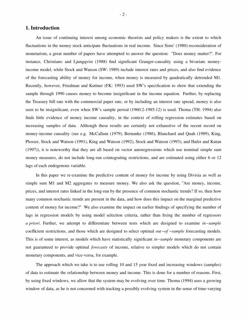
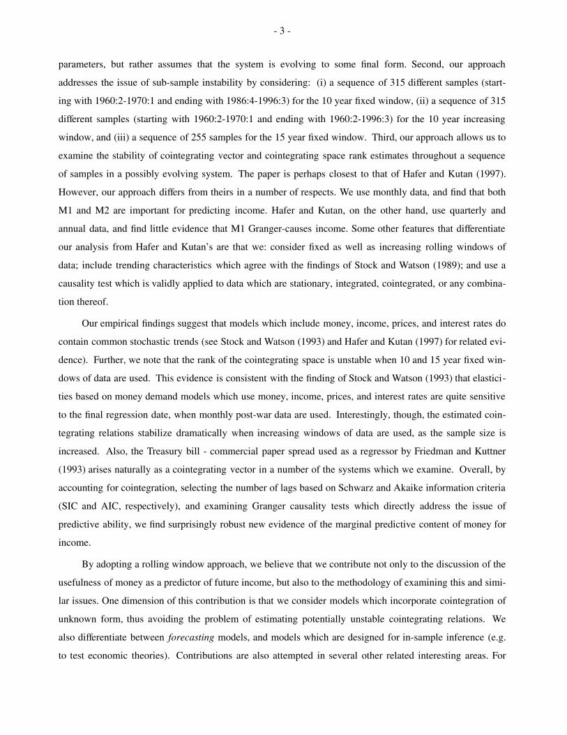
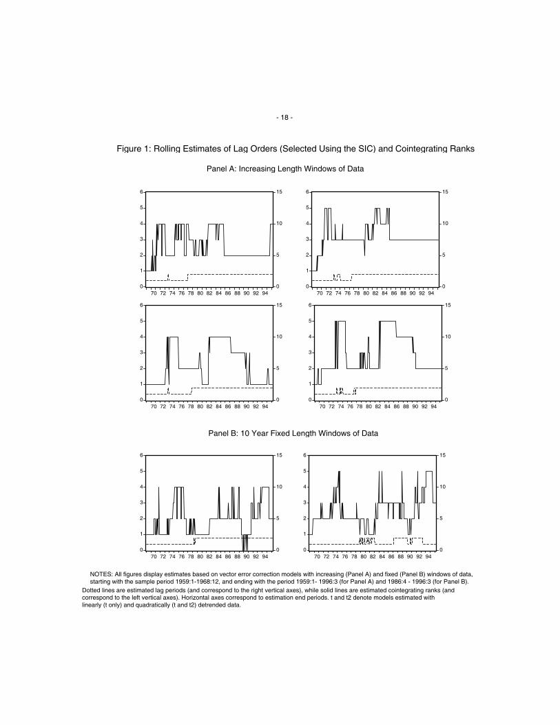
to numerous to list here, they are similar across all money measures, and are summarized in Figures 1 and 2,

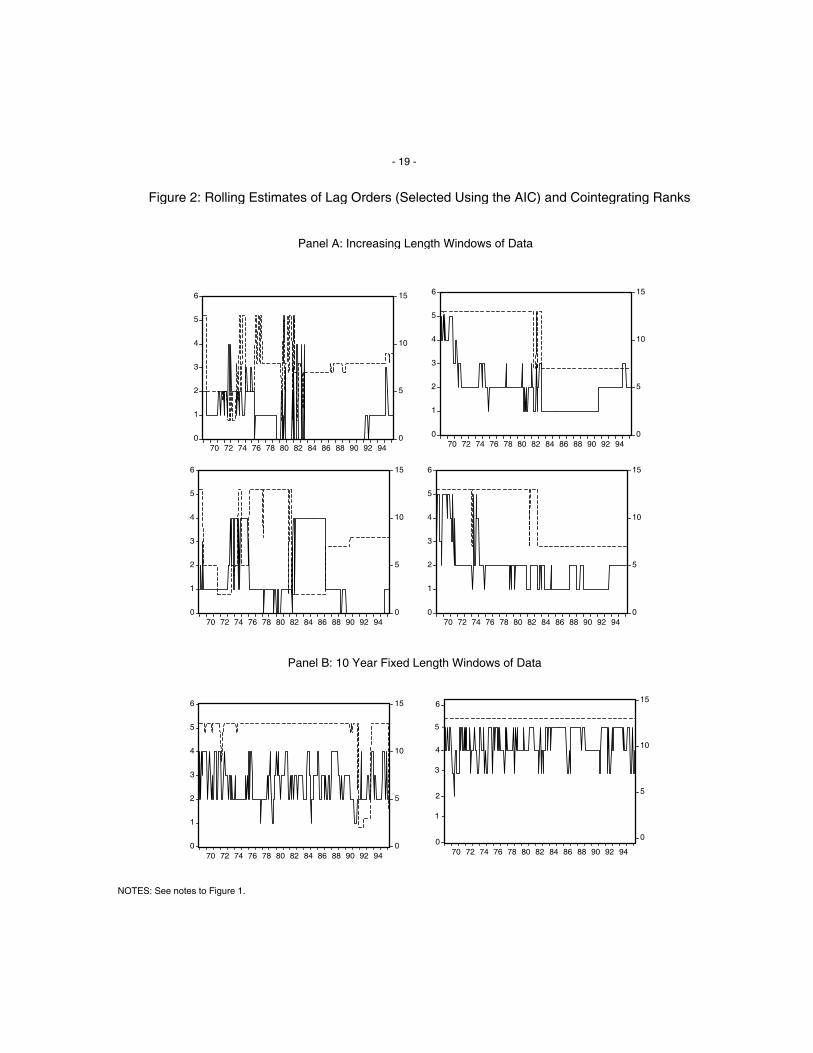
where estimation results based on the use of m 2t as the money measure are plotted. 5

insert Figures 1 and 2 about here

Figure 1, Panel A contains plots of estimated cointegrating space ranks and lag orders (based on the

SIC) for models estimated with increasing windows of data. Note that the cointegrating rank seems to sta-

bilize at two when the data are linearly detrended, and at one when the data are quadratically detrended,

when m 2t , yt , pt , and it are modeled. Thus, cointegrating rank estimates are dependent on the assumed

deterministic trend components in the model. This problem is not disimilar from the difficulty in testing for

trend versus difference stationarity in univariate series, and suggests that care needs to be taken at the intial

model specification stage of our analysis. Lag selection is not dependent on whether the data are linearly or

quadratically detrended. However, our models appear to become much more confused when the AIC is used

in place of the SIC to select lags (see Figure 2, Panel A), with respect to both cointegrating rank estimation

and lag selection. This suggests that stable models (with respect CI space rank and lag order) are more

easily specified when the more parsimonious SIC is used. When the commercial paper rate is added to our

models, the cointegrating rank increases by one, in all cases. This is interesting, as it suggests that the

paper-bill spread used by FK (1993) is a candidate error-correction term. This conjecture is confirmed rather

easily in the context of the five variable VEC model with lags selected by the SIC, with quadratically

detrended data, and with m 2t used as the money measure, for example, as each of the 75 most recent

increasing windows of data (i.e. samples from 1960:2-1990:1 increasing monthly to 1960:2-1996:3), one of

the two cointegrating vectors is ct it , based on a likelihood ratio test (see Johansen (1988, 1991)). Of

further note is that the null hypothesis that the other CI vector is (1 1 1 0 0) almost always fails to reject,

although confidence intervals are quite wide relative to those for the interest rate spread CI vector. (Actual

parameter estimates are available upon request.)

_______________5 Note that the right vertical axes of the graphs, which are used to denote the number of estimated lags for each

rolling regression model, run from 0 to 15 in Figure 1, and from -30 to 15 in Figure 2. This is done in order to ensurethat the plotted lines in each graph do not overlap.

- 8 -

Panel B of Figures 1 and 2 contains similar plots for 10 year fixed windows of data, but only for

linearly detrended data (results for quadratically detrended data are similar). It is clear that the cointegrating

rank evolves quite sporadically, and does not stabilize over time, regardless as to whether the SIC or the AIC

is used to select the number of lags. 6 Given the above discussion, we conclude that the 120 month samples

are too short to accurately estimate cointegrating spaces and ranks. Interestingly, this is the case even when

the order of the VEC model is only one or two (i.e. when the SIC is used to choose the lag length), suggest-

ing that in addition to a degrees of freedom (or confidence interval) problem, our shorter samples simply

don’t contain enough dynamic information to accurately estimate long-run relationships among the vari-

ables. When 15 year fixed windows of data are used, the picture that emerges is much the same as that illus-

trated in Panel B of Figures 1 and 2. There are two possible remedies to this apparent difficulty in pinning

down the cointegration in our fixed window models. First, longer samples of data can be used (e.g. use

increasing windows of data). Second, a method can be used to test for the marginal predictive content of

money for income which doesn’t require estimation of the cointegrating restrictions in the system. The

second approach is particularly appealing when it is suspected that the system may be evolving over time, so

that even the use of increasing windows of data may not enable us to precisely estimate CI vectors and CI

space ranks. In the next section we discuss these alternative testing approaches, and also consider a model

selection based approach as an alternative to in-sample based Granger causality testing.

4. Estimation and Testing

Least squares is used to estimate the parameters of the 40 VAR models given by equation (1), while

maximum likelihood is used to estimate 40 related VEC models given by the following equation:

xt = 0 + (t) + B (L)xt 1 + i =1r

izi,t 1 + t , (3)

where xt and (t) are as discussed above, t is a vector of innovations, zi,t 1 = ̂´xt 1, i=1,...,r, is a vector of

I(0) error-correction terms estimated in standard fashion using the methods proposed by Johansen (1988,

1991), r is the estimated rank of the cointegrating space, and B (L) is a matrix polynomial in the lag operator

L. As discussed above, the lag order of our models, say l, is chosen alternately using the SIC and the AIC. In

all cases, the number of lags for each endogenous variable in the system is the same. At this point, it should

perhaps be reiterated that (1) and (3) represent models for a single fixed sample period. As we are imple-

menting a rolling window approach, however, estimates of each of the parameters in equations (1) and (3),

_______________6 In one sense, these results are not surprising, given the evidence found by Gonzalo (1994) and Bewley, Orden,

Yang, and Fisher (1994), who discuss the small-sample tendency for maximum likelihood based procedures togenerate biased and leptokurtic distributions. Also, it is worth noting that empirical analysis has shown thatestimates of cointegrating spaces may differ, depending on which method of estimation is used (e.g. see Stock andWatson (1993)).

- 9 -

including the coefficients, l, and r, may vary from sample to sample. For example, for 10 year fixed windows

of data, 315 different sets of parameters are estimated. Corresponding to our above examination of rolling

cointegration rank and lag length estimates, 10 and 15 year fixed as well as 10 year increasing windows of

data are used in order to assess the extent to which fluctuations in money anticipate fluctuations in industrial

production. However, given our findings with regard to the instability of cointegrating rank estimates, we

wish to stress that the fixed window and the increasing window methods may yield quite different empirical

findings, particularly given our lack of knowledge concerning how rapidly the economy is evolving over

time. 7

Three different types of causality tests are constructed, the first two of which are based on classical

hypothesis testing principles. The first of these is the standard Wald test which is designed for stationary and

difference stationary data. This test statistic is constructed for all models estimated using equation (1). The

second test is the surplus lag regression test due to Dolado and Lütkepohl (1996) as well as Toda and

Yamamoto (1995). This is also a standard Wald test, but is based on a VAR model in levels, and does not

require pre-testing for cointegration, as models estimated in levels implicitly include cointegration of

unspecified form - a property which is not shared by difference VAR models. The test has the property that

nonstandard asymptotics that arise when standard Wald tests are applied to integrated and/or cointegrated

variables are forced in "surplus" coefficient matrices. The only requirement for the consistency of this test is

that the number of surplus lags "added" to the original VAR model is equal to or greater than the largest

order of integration of any of the variables in the system. Swanson, Ozildirim, and Pisu (SOP: 1996) show

that the surplus lag test has excellent finite sample size properties, particularly relative to standard Wald

tests when the variables in the system are cointegrated. However, due to the inefficient estimation of systems

with surplus lags, the finite sample power of the surplus lag test should be suspect. Further, a careful exami-

nation of the power functions of these types of tests still remains to be done, in particular to ensure that the

local power is not flat in most or all directions. Nevertheless, recall that our estimates of cointegrating space

ranks based on 10 and 15 year fixed windows of data are very erratic. This may be interpreted as evidence of

the imprecise nature of these small sample estimates, and supports the use of surplus lag regression tests,

which avoid the necessity of constructing cointegrating space estimates. Indeed, the loss of power associated

with inefficient estimation of surplus lags may be less than the loss of power associated with the imprecise

estimation of cointegrating spaces, were standard tests to be used. (SOP (1996) provide preliminary evi-

dence that this tradeoff is important when constructing Granger causality tests.)

_______________7 Granger (1996) points out that structural instability may be the most important problem facing forecasters today.

We take the approach of allowing for possible structural instability by using rolling windows.

- 10 -

Both of our classical Wald tests are based on testing for the significance of money in the income equa-

tion. However, Granger causality tests have a natural interpretation as tests of predictive ability. In this

sense, it may seem natural to use the results of causality tests when constructing forecasting models. How-

ever, any good forecasting model should be "tested" using some sort of ex ante forecasting experiment

before being implemented in any practical way. Along these lines, a reasonable alternative "test" for non-

causality could be to consider a set of different forecasting models, both with and without the variable whose

causal effect is being examined. These "competing" models could then be subjected to an ex ante forecast-

ing analysis and the "best" model chosen using some sort of out-of-sample model selection criterion. Then,

if the "best" model contains the variable of interest, noncausality is "rejected". Here, we consider a related

alternative to classical Wald tests which is based on model selection, noting that Granger, King, and White

(1995) suggest that although standard hypothesis testing has a role to play in terms of testing economic

theories, it is more difficult to justify using standard hypothesis tests for choosing between two competing

models. One reason for their concern is that one model must be selected as the null, and this model is often

the more parsimonious model (as in our case). However, it is often difficult to distinguish between the two

models (because of multicollinearity, near-identification, etc.), so that the null hypothesis may be unfairly

favored. For example, it is far from clear that pre-test significance levels of 5% and 1%, say, are optimal.

The use of model selection criteria neatly avoids the problem of how to arbitrarily choose significance lev-

els. Another advantage of the model selection approach is that it does not require specification of a correct

model for its valid application. Further, the probability of selecting the truly best model approaches one as

the sample size increases, if the model-selection approach is properly designed. This is contrary to the stan-

dard practice of fixing a test size, and rejecting the null hypothesis at that fixed size, regardless of sample

size. Swanson and White (1995, 1996) discuss these and related features of model selection, while SOP

(1996) show using Monte Carlo that predictive accuracy tests based on the AIC and the SIC have empirical

probabilities associated with selecting the wrong model which approach zero very quickly, even for sample

sizes of 100, 200, and 300 observations. Our approach is to use two complexity based likelihood criteria, the

AIC and the SIC, where:

AIC = T log | ̂ | + 2 f and SIC = T log | ̂ | + f log(T) ,

where f is the total number of parameters in the system (if we are measuring the causal effect of some

variable(s) on a group of more than one other variable), or, f is the number of parameters in the single equa-

tion of interest (when the group being examined is a single variable). Similarly, ̂ is some standard estimate

of the error covariance matrix, which is scalar if only one equation in the system is being examined. The

AIC and SIC type tests (which we hereafter refer to as "predictive accuracy" tests) are implemented as fol-

lows. The statistics are calculated for VEC versions of the models both with and without money variables. 8_______________

8 For each rolling window of data, we use a standard 2 hypothesis test on the estimated cointegrating vectors in

- 11 -

If the "best" model contains any money variable(s), then we have direct evidence of the marginal predictive

content of money for income. 9

5. Empirical Results

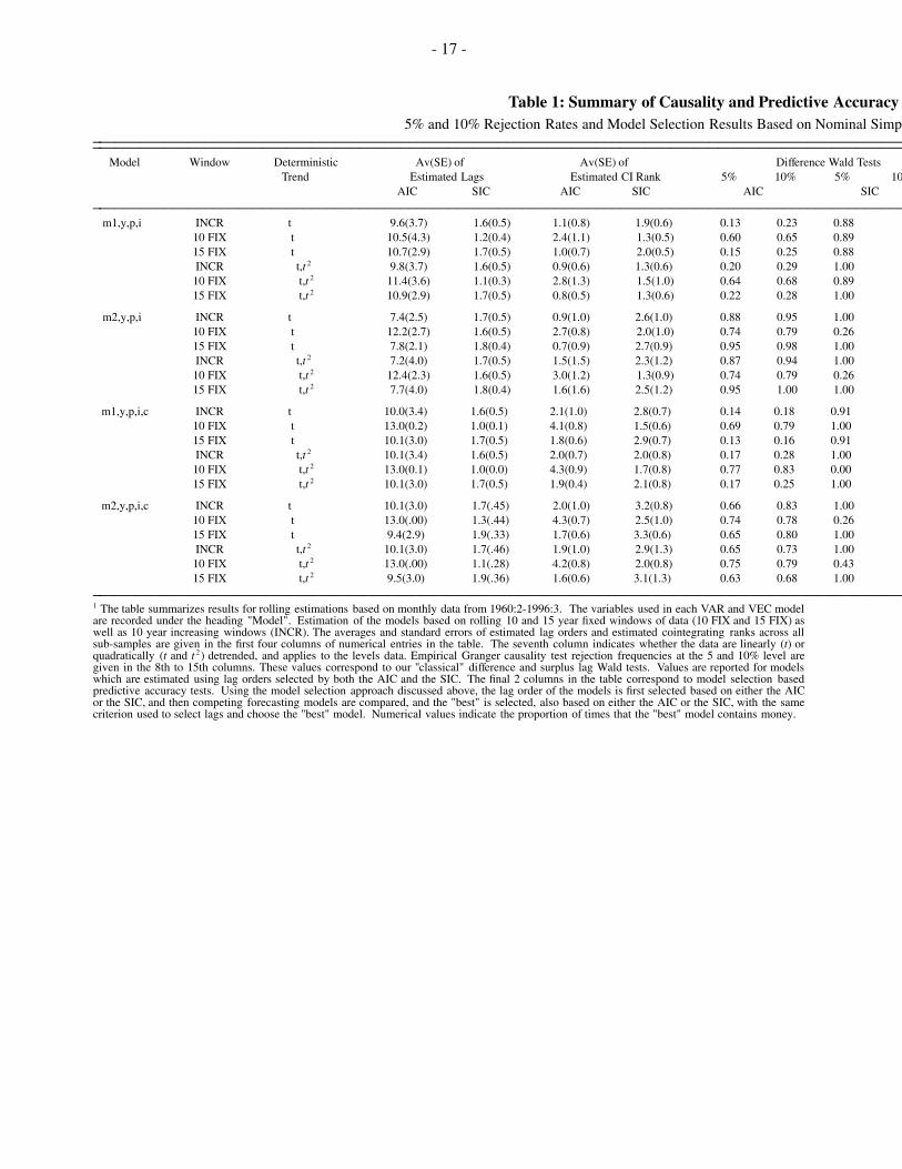
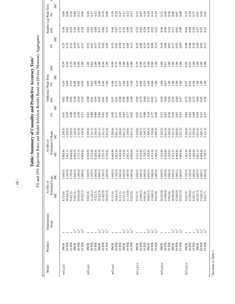
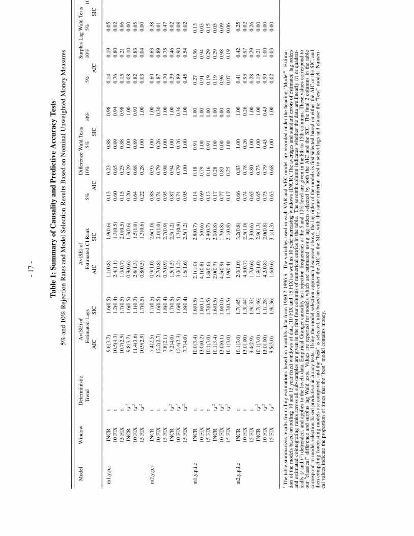
The results of the Granger causality and predictive accuracy tests are presented in Table 1 for the cases

where money is measured using m 1t and m 2t . A similar table based on dm 1t , dm 2t , and dm 3t has not been

included because the results are numerically very similar to those presented in Table 1. (The table is avail-

able upon request.) Table 1 is broken into four groups of six rows, each corresponding to a different choice

of variables. In turn, each set of variables is fit to VAR and VEC models using linearly and quadratically

detrended data, 10 year fixed, 15 year fixed, and 10 year increasing windows of data, and based on lag orders

chosen using both the AIC and the SIC. Entries in the table are rejection frequencies of the Granger non-

causality null (for standard Wald tests and surplus lag Wald tests, which we call our "classical" hypothesis

tests), and the percentage of times that the "best" model contains money (for the predictive accuracy tests).

insert Table 1 about here

Consider first the results based on standard Wald tests, which we call our "difference Wald tests".

When the AIC is used to select lags, rejection frequencies range from 63 to 100%, regardless of window

type and trend specification, for all models with m 2t . However, when m 1t is used, rejection frequencies are

much higher for the 10 year fixed window (around 65%) than for the other windows (where frequencies are

often as low as 15%). This may suggest that models with m 1t are evolving quite rapidly, so that the longer

windows are less apt to effectively capture the money-income relationship. On the other hand, a degrees of

freedom argument may also account for the apparent strength of the 10 year fixed window rejection frequen-

cies, particularly as the AIC tends to overselect the lag order. The degrees of freedom argument is made

even more believable by noting that rejection frequencies skyrocket to near unity for all longer windows

when the SIC is used to select lag order. Paradoxically, though, the only low rejection frequencies for the

cases where SIC is used are for m 2t and the 10 year fixed window! In one sense, this constitutes evidence

which is rather the opposite of when the AIC is used, at least with respect to m 2t . Thus, our evidence is

rather mixed based on difference Wald tests. However, we know that the variables are cointegrated, and

hence test bias may be driving our results, particularly for the cases where lag orders are chosen using the

SIC, given that the SIC selects more parsimonious models than the AIC. This is one of the reasons why we

_______________the system to determine whether money has a nonzero weight in the cointegrating vector(s). This in turn allows us todetermine which cointegrating vectors to include in our more parsimonious model which excludes money.

9 Thus far, we have not differentiated between "short-" and "long-run" predictive ability. However, if we viewcointegrating restrictions as corresponding to long-run relationships (see e.g. Granger an Lin (1994)), and laggeddifference variables as corresponding to short-run relationships (as has been done elsewhere), then our differencevariable Wald tests might be viewed as testing for short-run predictive ability, while the rest of our tests could beviewed as simultaneously testing for both short- and long-run predictive ability.

- 12 -

also estimate surplus lag Wald tests. As mentioned above, these tests are designed to incorporate cointegra-

tion of unspecified form at the model estimation stage, and are based on levels VAR models. Because it is

so important to include sufficient "surplus" lags (in order that standard asymptotic critical values can be

used), the AIC may be preferable for selecting lag order for these tests. Interestingly, cursory examination of

the rejection frequencies in the AIC columns suggests that rejection rates are high only for 10 year fixed

window cases. Since the 10 year fixed window cases are suspect (given the above discussion, and due to an

even more severe degrees of freedom problem than was the case for the difference Wald tests), we must ten-

tatively conclude that there is little evidence of the marginal predictive content of money for income, based

on surplus lag tests. However, these tests may suffer from reduced finite sample power. Furthermore, we

know that our difference VAR Wald tests are subject to finite sample size bias. Indeed, it is quite likely that

these two related, but opposite problems account in large part for the disparity in our findings based on the

two classical Granger noncausality tests. This is one of the reasons why we use a model selection approach

in addition to Granger causality tests.

As outlined above, our model selection based predictive accuracy tests are based on the premise of

choosing the "best" forecasting model. For this reason, we might wish to entertain the rather widely held

notion that more parsimonious models (i.e. those specified using the SIC to select lag order) often forecast

better. In order to evaluate this hypothesis, we carried out a series of simple experiments. Using all of our

different windows of data, we fit levels VAR models, difference VAR models, and VEC models to 0.7*T of

each rolling sample of data. The remaining 0.3*T observations in each rolling sample were used to construct

a sequence a rolling one-step ahead ex ante forecasts of income. A total of 0.3*T new models, cointegrating

spaces, etc. were estimated for each roll of the data window, in order to construct the 0.3*T length one-step

ahead forecast sequences (so that many thousands of models were estimated in all). In all cases, competing

models were estimated which used the AIC and the SIC to select lag order, and Diebold and Mariano (1995)

loss differential tests statistics were constructed for each window of data (based on mean square forecast

error, mean absolute forecast error deviation, and mean absolute percentage forecast error - see Swanson and

White (1996) for details of these statistics) to determine whether one lag selection procedure resulted in

better forecast models, in the sense of quadratic forecast error loss. The experiment was repeated for both

trend specifications. As might be expected, the results based on these ex ante experiments suggest that the

SIC is preferred by a more than a 2 to 1 ratio, regardless of model specification. Summarizing our findings,

the AIC tends to pick the best out-of-sample model around 0-20% of the time, the SIC around 30-65% of the

time, and neither model is preferred around 30-50% of the time. (To save on space, tabulated results are not

included.) Thus, we have direct evidence that the SIC is preferable when constructing one-step ahead fore-

casting models of income. For this reason, we prefer predictive accuracy tests which use models estimated

- 13 -

with lag orders chosen using the SIC.

The results based on our model selection approach are gathered under the heading "predictive accu-

racy tests" in Table 1. Note that for the SIC version of this test, both lag order and the "best" forecasting

model are selected using the SIC. Analogously, the AIC version of the test uses the AIC for lag selection and

for choosing the "best" forecasting model. Interestingly, using the SIC results in the selection of models

which include money close to 100% of the time, regardless of variables, trend specification, window, etc.

The exception to this result is the 10 year fixed window of data, which again appears to be too short to offer

relevant evidence in our experiments, at least when m 2t is used. Since the SIC can be interpreted as a statis-

tic useful for selecting optimal forecasting models, we have rather strong new evidence of the marginal

predictive content of money for income. This evidence comes to light in part by examining carefully the

shortcomings of other tests of Granger noncausality in the presence of cointegrated data, and is clearly

robust to sample period, as long as the data horizon used is sufficiently long. Further, as the VEC models

estimated for our predictive accuracy tests generally include a cointegrating vector which is the ct - it

spread, we have some evidence that Friedman and Kuttner’s (1993) preferred model (see above discussion)

actually supports a finding of money income causality, when viewed through a rolling window. Also, esti-

mation of Thoma’s (1995) preferred model (which is essentially a difference VAR model, and can be exam-

ined using the difference Wald test) leads to strong evidence of the marginal predictive content of money for

income, subject to the above test bias criticism, of course. Finally, we come back to Stock and Watson’s

(1989) original findings based on systems such as those examined here. Our evidence, which is based on a

somewhat broader examination of many related models, clearly supports their original finding of the predic-

tive ability of money for income.

6. Summary and Concluding Remarks

We have used a rolling window approach based on fixed and increasing samples of data to investigate

the extent to which fluctuations in the money stock anticipate fluctuations in real output. Based on our

empirical analysis, we offer the following conclusions. First, it is far from clear that money does not have

significant predictive power for income. When either Divisia monetary aggregates or simple sum money

measures are used as the monetary aggregate in systems with income, prices, and interest rates, the predic-

tive content of money is significant for virtually all of the rolling samples between 1960:2 and 1994:6. How-

ever, this result is somewhat dependent upon the type of test which is used. For example, predictive accu-

racy tests which are based on a model selection approach to selecting "best" forecasting models are shown

to overwhelmingly favour models with money, even when additional regressors, such as the commercial

paper - T-bill rate spread are added to our models. Other hypothesis tests, while less favourable to money,

are shown to be fraught with potential problems. In particular, we note that Wald tests based on differenced

- 14 -

data VAR models may be biased when the true data generating process is a VEC model. Surplus lag Wald

tests, on the other hand, while accounting for cointegration of unspecified form, may be affected by reduced

finite sample power.

Second, the systems of variables examined appear to evolve to some final form over time, in particular

with respect to the characterization of the basis of the cointegration space. More precisely, we find no

advantage to considering shorter 10 year fixed windows of data. The systems are particularly stable when

the SIC is used to select the lag order. Furthermore, the SIC is preferred to the AIC, when used to select the

lag order of VEC models used to produce one-step ahead ex ante forecasts of income.

The work here is merely a starting point. A wide variety of further questions present themselves for

subsequent research, both theoretical and empirical. On the theoretical side, it is of interest to establish the

statistical properties of surplus lag Wald tests, particularly with respect to test power. Interesting empirical

projects include applying the analysis in this paper to the examination of impulse response functions, inves-

tigating the predictive power of money for income using alternative measures of predictive ability (such as

rolling window forecast error-variance decompositions in a vector error-correction system), constructing

true ex ante model selection based tests for the predictive ability of money, and expanding the endogenous

systems analyzed by including labor demand channels (as measured by the unemployment rate), for exam-

ple.

- 15 -

References

Anderson, R.G., B. Jones, and T. Nesmith, 1996, Building new monetary services indices: concepts, metho-dology and data, Working paper (Federal Reserve Bank of St. Louis, St. Louis, MI).

Barnett, W.A., 1978, The user cost of money, Economic Letters 1, 145-149.

Barnett, W.A., 1980, Economic monetary aggregates: an application of index number and aggregationtheory, Journal of Econometrics 14, 11-48.

Barnett, W.A., 1990, Developments in monetary aggregation theory, Journal of Policy Modeling 12, 205-257.

Bernanke, B.S., 1986, Alternative explanations of the money-income correlation, Carnegie-RochesterConference Series on Public Policy 25, 49-100.

Bewley, R., D. Orden, M. Xang and L.A. Fisher, 1994, Comparison of Box-Tiao and Johansen canonicalestimators of cointegrating vector in VEC(1) models, Journal of Econometrics 64, 3-27.

Blanchard, O.J. and D. Quah, 1989, The dynamic effects of aggregate demand and supply disturbances,American Economic Review 79, 655-673.

Christiano, L.J. and L. Ljungqvist, 1988, Money does Granger-cause output in the bivariate money-outputrelation, Journal of Monetary Economics 22, 217-235.

Diebold, F.X. and R.S. Mariano, 1995, Comparing predictive accuracy, Journal of Business and EconomicStatistics 13, 253-263.

Dolado, J.J. and H. Lütkepohl, 1996, Making Wald tests work for cointegrated VAR systems, EconometricReviews 15, 369-386.

Friedman, B.M. and K.N. Kuttner, 1993, Another look at the evidence on money-income causality, Journalof Econometrics 57, 189-203.

Gonzalo, J., 1994, Five alternative methods of estimating long-run equilibrium relationships, Journal ofEconometrics 60, 203-233.

Granger, C.W.J., 1996, Can we improve the perceived quality of economic forecasts?, Journal of AppliedEconometrics 11, 455-473.

Granger, C.W.J., M.L. King and H. White, 1995, Comments on testing economic theories and the use ofmodel selection criteria, Journal of Econometrics 67, 173-187.

Granger, C.W.J., and J.-L. Lin, 1995, Causality in the long run, Econometric Theory 11, 530-536.

Granger, C.W.J., and T. Teräsvirta, 1993, Modeling nonlinear economic relationships (Oxford, New York,N.Y.).

Hafer, R.W. and D.W. Jansen, 1991, The demand for money in the United States: evidence from cointegra-tion tests, Journal of Money, Credit, and Banking 23, 155-168.

Hafer, R.W. and A.M. Kutan, 1997, More evidence on the money-output relationship, Economic Inquiry 35,48-58.

Johansen, S., 1988, Statistical analysis of cointegrating vectors, Journal of Economic Dynamics and Control12, 231-254.

Johansen, S., 1991, Estimation and hypothesis testing of cointegration vectors in Gaussian vector autoregres-sive models, Econometrica 59, 1551-1580.

King, R.G., C.I. Plosser, J.H. Stock and Mark M. Watson, 1991, Stochastic trends and economic fluctuations,American Economic Review 81, 819-840.

King, R.G. and M.M. Watson, 1992, Testing long run neutrality, Working Paper (National Bureau of

- 16 -

Economic Research, Boston, MA).

McCallum, B.T., 1979, The current state of the policy-ineffectiveness debate, American Economic Review69, 240-245.

Potter, S., 1995, A nonlinear approach to US GNP, Journal of Applied Econometrics 10, 109-125.

Sims, C.A., 1980, Comparison of interwar and postwar cycles: monetarism reconsidered, AmericanEconomic Review 70, 250-257.

Stock, J.H. and M.M. Watson, 1989, Interpreting the evidence on money-income causality, Journal ofEconometrics 40, 161-181.

Stock, J.H. and M.M. Watson, 1993, A simple estimator of cointegrating vectors in higher order integratedsystems, Econometrica 61, 783-820.

Swanson, N.R., Ozyildirim, A. and M. Pisu, 1996, A comparison of alternative causality and predictiveaccuracy tests in the presence of integrated and cointegrated economic variables, Working paper (Pennsyl-vania State University, University Park, PA).

Swanson, N.R. and H. White, 1995, A model selection approach to assessing the information in the termstructure using linear models and artificial neural networks, Journal of Business and Economic Statistics 13,265-275.

Swanson, N.R. and H. White, 1996, A model selection approach to real-time macroeconomic forecastingusing linear models and artificial neural networks, Review of Economics and Statistics, forthcoming.

Thoma, M.A., 1994, Subsample instability and asymmetries in money-income causality, Journal ofEconometrics 64, 279-306.

Toda, Hiro Y. and Taku Yamamoto, 1995, Statistical inference in vector autoregressions with possiblyintegrated processes, Journal of Econometrics 66, 225-250.

- 17 -

Table 1: Summary of Causality and Predictive Accuracy5% and 10% Rejection Rates and Model Selection Results Based on Nominal Simpl

Model Window Deterministic Av(SE) of Av(SE) of Difference Wald TestsTrend Estimated Lags Estimated CI Rank 5% 10% 5% 10

AIC SIC AIC SIC AIC SICm1,y,p,i INCR t 9.6(3.7) 1.6(0.5) 1.1(0.8) 1.9(0.6) 0.13 0.23 0.88

10 FIX t 10.5(4.3) 1.2(0.4) 2.4(1.1) 1.3(0.5) 0.60 0.65 0.8915 FIX t 10.7(2.9) 1.7(0.5) 1.0(0.7) 2.0(0.5) 0.15 0.25 0.88INCR t,t 2 9.8(3.7) 1.6(0.5) 0.9(0.6) 1.3(0.6) 0.20 0.29 1.0010 FIX t,t 2 11.4(3.6) 1.1(0.3) 2.8(1.3) 1.5(1.0) 0.64 0.68 0.8915 FIX t,t 2 10.9(2.9) 1.7(0.5) 0.8(0.5) 1.3(0.6) 0.22 0.28 1.00

m2,y,p,i INCR t 7.4(2.5) 1.7(0.5) 0.9(1.0) 2.6(1.0) 0.88 0.95 1.0010 FIX t 12.2(2.7) 1.6(0.5) 2.7(0.8) 2.0(1.0) 0.74 0.79 0.2615 FIX t 7.8(2.1) 1.8(0.4) 0.7(0.9) 2.7(0.9) 0.95 0.98 1.00INCR t,t 2 7.2(4.0) 1.7(0.5) 1.5(1.5) 2.3(1.2) 0.87 0.94 1.0010 FIX t,t 2 12.4(2.3) 1.6(0.5) 3.0(1.2) 1.3(0.9) 0.74 0.79 0.2615 FIX t,t 2 7.7(4.0) 1.8(0.4) 1.6(1.6) 2.5(1.2) 0.95 1.00 1.00

m1,y,p,i,c INCR t 10.0(3.4) 1.6(0.5) 2.1(1.0) 2.8(0.7) 0.14 0.18 0.9110 FIX t 13.0(0.2) 1.0(0.1) 4.1(0.8) 1.5(0.6) 0.69 0.79 1.0015 FIX t 10.1(3.0) 1.7(0.5) 1.8(0.6) 2.9(0.7) 0.13 0.16 0.91INCR t,t 2 10.1(3.4) 1.6(0.5) 2.0(0.7) 2.0(0.8) 0.17 0.28 1.0010 FIX t,t 2 13.0(0.1) 1.0(0.0) 4.3(0.9) 1.7(0.8) 0.77 0.83 0.00 015 FIX t,t 2 10.1(3.0) 1.7(0.5) 1.9(0.4) 2.1(0.8) 0.17 0.25 1.00

m2,y,p,i,c INCR t 10.1(3.0) 1.7(.45) 2.0(1.0) 3.2(0.8) 0.66 0.83 1.0010 FIX t 13.0(.00) 1.3(.44) 4.3(0.7) 2.5(1.0) 0.74 0.78 0.2615 FIX t 9.4(2.9) 1.9(.33) 1.7(0.6) 3.3(0.6) 0.65 0.80 1.00INCR t,t 2 10.1(3.0) 1.7(.46) 1.9(1.0) 2.9(1.3) 0.65 0.73 1.0010 FIX t,t 2 13.0(.00) 1.1(.28) 4.2(0.8) 2.0(0.8) 0.75 0.79 0.4315 FIX t,t 2 9.5(3.0) 1.9(.36) 1.6(0.6) 3.1(1.3) 0.63 0.68 1.00

1 The table summarizes results for rolling estimations based on monthly data from 1960:2-1996:3. The variables used in each VAR and VEC modelare recorded under the heading "Model". Estimation of the models based on rolling 10 and 15 year fixed windows of data (10 FIX and 15 FIX) aswell as 10 year increasing windows (INCR). The averages and standard errors of estimated lag orders and estimated cointegrating ranks across allsub-samples are given in the first four columns of numerical entries in the table. The seventh column indicates whether the data are linearly (t) orquadratically (t and t 2) detrended, and applies to the levels data. Empirical Granger causality test rejection frequencies at the 5 and 10% level aregiven in the 8th to 15th columns. These values correspond to our "classical" difference and surplus lag Wald tests. Values are reported for modelswhich are estimated using lag orders selected by both the AIC and the SIC. The final 2 columns in the table correspond to model selection basedpredictive accuracy tests. Using the model selection approach discussed above, the lag order of the models is first selected based on either the AICor the SIC, and then competing forecasting models are compared, and the "best" is selected, also based on either the AIC or the SIC, with the samecriterion used to select lags and choose the "best" model. Numerical values indicate the proportion of times that the "best" model contains money.

- 16

-

Tab

le:Su

mm

ary

ofC

ausa

lity

and

Pre

dict

ive

Acc

urac

yTes

ts1

5%an

d10

%R

ejec

tion

Rat

esan

dM

odel

Sele

ctio

nR

esul

tsB

ased

onD

ivis

iaM

onet

ary

Agg

rega

tes

Mod

elW

indo

wD

eter

min

istic

Av(

SE)o

fA

v(SE

)of

Dif

fere

nce

Wal

dTe

sts

Surp

lus

Lag

Wal

dTe

sts

Tren

dE

stim

ated

Lag

sE

stim

ated

CI

Ran

k5%

10%

5%10

%5%

10%

5%1

AIC

SIC

AIC

SIC

AIC

SIC

AIC

SIC

m1,

y,p,

iIN

CR

t8.

7(3.

0)1.

6(0.

5)0.

8(0.

8)2.

2(0.

5)0.

010.

020.

190.

790.

250.

300.

0810

FIX

t10

.4(4

.4)

1.3(

0.5)

2.4(

1.1)

1.2(

0.5)

0.55

0.60

0.89

0.94

0.70

0.82

0.08

15FI

Xt

9.4(

2.5)

1.7(

0.4)

0.6(

0.6)

2.2(

0.5)

0.00

0.01

0.19

0.79

0.22

0.25

0.10

INC

Rt,t

29.

4(3.

2)1.

6(0.

5)0.

8(0.

5)1.

1(0.

4)0.

200.

280.

981.

000.

300.

360.

0010

FIX

t,t2

10.9

(4.0

)1.

2(0.

4)2.

7(1.

3)1.

3(1.

0)0.

590.

640.

890.

940.

770.

850.

1215

FIX

t,t2

10.2

(2.7

)1.

8(0.

4)0.

8(0.

4)1.

1(0.

4)0.

210.

250.

981.

000.

210.

240.

00

m2,

y,p,

iIN

CR

t9.

0(2.

4)1.

6(0.

5)0.

5(0.

9)2.

3(0.

6)0.

830.

900.

991.

000.

520.

620.

2610

FIX

t11

.1(4

.1)

1.5(

0.5)

2.7(

1.0)

2.1(

1.1)

0.80

0.81

0.62

0.64

0.83

0.83

0.17

15FI

Xt

9.2(

2.3)

1.8(

0.4)

0.2(

0.5)

2.3(

0.4)

0.88

0.94

1.00

1.00

0.57

0.68

0.32

INC

Rt,t

210

.1(2

.5)

1.6(

0.5)

1.0(

1.0)

2.6(

1.1)

0.86

0.95

1.00

1.00

0.10

0.33

0.00

10FI

Xt,t

211

.4(3

.9)

1.3(

0.5)

2.7(

1.3)

1.5(

1.1)

0.81

0.81

0.46

0.46

0.85

0.86

0.19

15FI

Xt,t

210

.2(2

.5)

1.8(

0.4)

0.7(

0.8)

2.9(

1.0)

0.86

0.94

1.00

1.00

0.05

0.33

0.00

m3,

y,p,

iIN

CR

t8.

1(1.

6)1.

6(0.

5)0.

6(0.

8)2.

2(0.

6)0.

950.

970.

960.

990.

530.

660.

3910

FIX

t10

.8(4

.2)

1.5(

0.5)

2.8(

1.0)

2.0(

1.1)

0.77

0.81

0.72

0.75

0.83

0.87

0.22

15FI

Xt

8.1(

1.1)

1.8(

0.4)

0.4(

0.6)

2.2(

0.4)

0.96

0.98

0.97

1.00

0.59

0.71

0.47

INC

Rt,t

29.

1(2.

2)1.

6(0.

5)1.

1(0.

9)2.

6(1.

2)0.

850.

981.

001.

000.

150.

310.

1110

FIX

t,t2

11.1

(4.0

)1.

4(0.

5)2.

9(1.

3)1.

1(0.

6)0.

770.

800.

690.

690.

850.

900.

2215

FIX

t,t2

9.2(

2.0)

1.8(

0.4)

0.9(

0.6)

2.8(

1.1)

0.82

0.98

1.00

1.00

0.13

0.29

0.13

m1,

y,p,

i,cIN

CR

t9.

7(3.

3)1.

6(0.

5)2.

1(1.

1)3.

1(0.

6)0.

030.

050.

190.

790.

250.

320.

1510

FIX

t13

.0(0

.2)

1.0(

0.2)

4.2(

0.8)

1.5(

0.7)

0.71

0.79

0.90

0.90

0.88

0.92

0.07

15FI

Xt

9.9(

3.0)

1.8(

0.4)

1.7(

0.7)

3.1(

0.7)

0.00

0.00

0.19

0.79

0.19

0.24

0.18

INC

Rt,t

210

.0(3

.2)

1.6(

0.5)

2.1(

0.8)

1.9(

0.5)

0.14

0.23

1.00

1.00

0.29

0.34

0.16

10FI

Xt,t

213

.0(0

.1)

1.0(

0.0)

4.3(

1.0)

1.7(

0.8)

0.77

0.82

0.00

0.00

0.90

0.93

0.14

15FI

Xt,t

29.

9(3.

0)1.

8(0.

4)1.

9(0.

3)1.

9(0.

5)0.

060.

171.

001.

000.

190.

230.

19

m2,

y,p,

i,cIN

CR

t10

.4(2

.8)

1.6(

0.5)

1.5(

1.0)

3.2(

0.5)

0.51

0.54

1.00

1.00

0.18

0.26

0.21

10FI

Xt

13.0

(0.0

)1.

2(0.

4)4.

2(0.

8)2.

6(1.

0)0.

820.

860.

670.

670.

980.

980.

0815

FIX

t9.

9(2.

8)1.

8(0.

4)1.

2(0.

6)3.

2(0.

4)0.

560.

561.

001.

000.

070.

160.

26IN

CR

t,t2

10.9

(2.8

)1.

6(0.

5)1.

9(1.

2)3.

3(1.

3)0.

480.

551.

001.

000.

170.

170.

0010

FIX

t,t2

13.0

(0.0

)1.

0(0.

1)4.

4(0.

8)2.

0(0.

8)0.

810.

841.

001.

000.

920.

920.

0715

FIX

t,t2

10.5

(2.9

)1.

8(0.

4)1.

6(0.

8)3.

5(1.

2)0.

450.

471.

001.

000.

000.

000.

00

m3,

y,p,

i,cIN

CR

t9.

6(2.

9)1.

7(0.

5)1.

8(1.

0)3.

2(0.

6)0.

640.

720.

970.

990.

490.

640.

2310

FIX

t12

.9(0

.6)

1.2(

0.4)

4.3(

0.8)

2.5(

1.1)

0.82

0.85

0.92

0.92

0.96

0.98

0.10

15FI

Xt

8.9(

2.7)

1.8(

0.4)

1.4(

0.6)

3.2(

0.4)

0.68

0.72

0.98

1.00

0.38

0.56

0.27

INC

Rt,t

210

.2(2

.7)

1.6(

0.5)

2.0(

1.1)

3.0(

1.4)

0.64

0.66

1.00

1.00

0.29

0.37

0.01

10FI

Xt,t

213

.0(0

.2)

1.0(

0.1)

4.4(

0.8)

1.6(

0.7)

0.83

0.85

1.00

1.00

0.94

0.97

0.04

15FI

Xt,t

29.

6(2.

7)1.

8(0.

4)1.

7(0.

7)3.

1(1.

4)0.

570.

581.

001.

000.

130.

230.

01

1Se

eno

tes

toTa

ble

1.

- 17

-

Tab

le1:

Sum

mar

yof

Cau

salit

yan

dPre

dict

ive

Acc

urac

yTes

ts1

5%an

d10

%R

ejec

tion

Rat

esan

dM

odel

Sele

ctio

nR

esul

tsB

ased

onN

omin

alU

nwei

ghte

dM

oney

Mea

sure

s

Mod

elW

indo

wD

eter

min

istic

Av(

SE)o

fA

v(SE

)of

Dif

fere

nce

Wal

dTe

sts

Surp

lus

Lag

Wal

dTe

sts

Tren

dE

stim

ated

Lag

sE

stim

ated

CI

Ran

k5%

10%

5%10

%5%

10%

5%1 0

AIC

SIC

AIC

SIC

AIC

SIC

AIC

SIC

m1,

y,p,

iIN

CR

t9.

6(3.

7)1.

6(0.

5)1.

1(0.

8)1.

9(0.

6)0.

130.

230.

880.

980.

140.

190.

0510

FIX

t10

.5(4

.3)

1.2(

0.4)

2.4(

1.1)

1.3(

0.5)

0.60

0.65

0.89

0.94

0.76

0.80

0.02

15FI

Xt

10.7

(2.9

)1.

7(0.

5)1.

0(0.

7)2.

0(0.

5)0.

150.

250.

880.

980.

150.

210.

06IN

CR

t,t2

9.8(

3.7)

1.6(

0.5)

0.9(

0.6)

1.3(

0.6)

0.20

0.29

1.00

1.00

0.08

0.10

0.00

10FI

Xt,t

211

.4(3

.6)

1.1(

0.3)

2.8(

1.3)

1.5(

1.0)

0.64

0.68

0.89

0.93

0.82

0.83

0.05

15FI

Xt,t

210

.9(2

.9)

1.7(

0.5)

0.8(

0.5)

1.3(

0.6)

0.22

0.28

1.00

1.00

0.03

0.04

0.00

m2,

y,p,

iIN

CR

t7.

4(2.

5)1.

7(0.

5)0.

9(1.

0)2.

6(1.

0)0.

880.

951.

001.

000.

600.

630.

3810

FIX

t12

.2(2

.7)

1.6(

0.5)

2.7(

0.8)

2.0(

1.0)

0.74

0.79

0.26

0.30

0.87

0.89

0.01

15FI

Xt

7.8(

2.1)

1.8(

0.4)

0.7(

0.9)

2.7(

0.9)

0.95

0.98

1.00

1.00

0.70

0.75

0.47

INC

Rt,t

27.

2(4.

0)1.

7(0.

5)1.

5(1.

5)2.

3(1.

2)0.

870.

941.

001.

000.

390.

460.

0210

FIX

t,t2

12.4

(2.3

)1.

6(0.

5)3.

0(1.

2)1.

3(0.

9)0.

740.

790.

260.

360.

890.

900.

0815

FIX

t,t2

7.7(

4.0)

1.8(

0.4)

1.6(

1.6)

2.5(

1.2)

0.95

1.00

1.00

1.00

0.45

0.54

0.02

m1,

y,p,

i,cIN

CR

t10

.0(3

.4)

1.6(

0.5)

2.1(

1.0)

2.8(

0.7)

0.14

0.18

0.91

1.00

0.27

0.36

0.13

10FI

Xt

13.0

(0.2

)1.

0(0.

1)4.

1(0.

8)1.

5(0.

6)0.

690.

791.

001.

000.

910.

940.

0315

FIX

t10

.1(3

.0)

1.7(

0.5)

1.8(

0.6)

2.9(

0.7)

0.13

0.16

0.91

1.00

0.19

0.29

0.15

INC

Rt,t

210

.1(3

.4)

1.6(

0.5)

2.0(

0.7)

2.0(

0.8)

0.17

0.28

1.00

1.00

0.19

0.29

0.05

10FI

Xt,t

213

.0(0

.1)

1.0(

0.0)

4.3(

0.9)

1.7(

0.8)

0.77

0.83

0.00

0.00

0.96

0.98

0.09

15FI

Xt,t

210

.1(3

.0)

1.7(

0.5)

1.9(

0.4)

2.1(

0.8)

0.17

0.25

1.00

1.00

0.07

0.19

0.06

m2,

y,p,

i,cIN

CR

t10

.1(3

.0)

1.7(

.45)

2.0(

1.0)

3.2(

0.8)

0.66

0.83

1.00

1.00

0.41

0.42

0.25

10FI

Xt

13.0

(.00

)1.

3(.4

4)4.

3(0.

7)2.

5(1.

0)0.

740.

780.

260.

260.

950.

970.

0215

FIX

t9.

4(2.

9)1.

9(.3

3)1.

7(0.

6)3.

3(0.

6)0.

650.

801.

001.

000.

280.

290.

26IN

CR

t,t2

10.1

(3.0

)1.

7(.4

6)1.

9(1.

0)2.

9(1.

3)0.

650.

731.

001.

000.

190.

210.

0010

FIX

t,t2

13.0

(.00

)1.

1(.2

8)4.

2(0.

8)2.

0(0.

8)0.

750.

790.

430.

430.

991.

000.

0015

FIX

t,t2

9.5(

3.0)

1.9(

.36)

1.6(

0.6)

3.1(

1.3)

0.63

0.68

1.00

1.00

0.02

0.03

0.00

1T

heta

ble

sum

mar

izes

resu

ltsfo

rro

lling

estim

atio

nsba

sed

onm

onth

lyda

tafr

om19

60:2

-199

6:3.

The

vari

able

sus

edin

each

VA

Ran

dV

EC

mod

elar

ere

cord

edun

der

the

head

ing

"Mod

el".

Est

ima-

tion

ofth

em

odel

sba

sed

onro

lling

10an

d15

year

fixed

win

dow

sof

data

(10

FIX

and

15FI

X)a

sw

ell

as10

year

incr

easi

ngw

indo

ws

(IN

CR

).T

heav

erag

esan

dst

anda

rder

rors

ofes

timat

edla

gor

ders

and

estim

ated

coin

tegr

atin

gra

nks

acro

ssal

lsu

b-sa

mpl

esar

egi

ven

inth

efir

stfo

urco

lum

nsof

num

eric

alen

trie

sin

the

tabl

e.T

hese

vent

hco

lum

nin

dica

tes

whe

ther

the

data

are

linea

rly

(t)

orqu

adra

t-ic

ally

(tan

dt2

)de

tren

ded,

and

appl

ies

toth

ele

vels

data

.Em

piri

cal

Gra

nger

caus

ality

test

reje

ctio

nfr

eque

ncie

sat

the

5an

d10

%le

vel

are

give

nin

the

8th

to15

thco

lum

ns.T

hese

valu

esco

rres

pond

toou

r"c

lass

ical

"di

ffere

nce

and

surp

lus

lag

Wal

dte

sts.

Val

ues

are

repo

rted

for

mod

els

whi

char

ees

timat

edus

ing

lag

orde

rsse

lect

edby

both

the

AIC

and

the

SIC

.T

hefin

al2

colu

mns

inth

eta

ble

corr

espo

ndto

mod

else

lect

ion

base

dpr

edic

tive

accu

racy

test

s.U

sing

the

mod

else

lect

ion

appr

oach

disc

usse

dab

ove,

the

lag

orde

rof

the

mod

els

isfir

stse

lect

edba

sed

onei

ther

the

AIC

orth

eSI

C,a

ndth

enco

mpe

ting

fore

cast

ing

mod

els

are

com

pare

d,an

dth

e"b

est"

isse

lect

ed,

also

base

don

eith

erth

eA

ICor

the

SIC

,with

the

sam

ecr

iteri

onus

edto

sele

ctla

gsan

dch

oose

the

"bes

t"m

odel

.N

umer

i-ca

lval

ues

indi

cate

the

prop

ortio

nof

times

that

the

"bes

t"m

odel

cont

ains

mon

ey.

0

1

2

3

4

5

6

0

5

10

15

70 72 74 76 78 80 82 84 86 88 90 92 940

1

2

3

4

5

6

0

5

10

15

70 72 74 76 78 80 82 84 86 88 90 92 94

0

1

2

3

4

5

6

0

5

10

15

70 72 74 76 78 80 82 84 86 88 90 92 940

1

2

3

4

5

6

0

5

10

15

70 72 74 76 78 80 82 84 86 88 90 92 94

0

1

2

3

4

5

6

0

5

10

15

70 72 74 76 78 80 82 84 86 88 90 92 940

1

2

3

4

5

6

0

5

10

15

70 72 74 76 78 80 82 84 86 88 90 92 94

Figure 1: Rolling Estimates of Lag Orders (Selected Using the SIC) and Cointegrating Ranks

Panel A: Increasing Length Windows of Data

Panel B: 10 Year Fixed Length Windows of Data

NOTES: All figures display estimates based on vector error correction models with increasing (Panel A) and fixed (Panel B) windows of data,starting with the sample period 1959:1-1968:12, and ending with the period 1959:1- 1996:3 (for Panel A) and 1986:4 - 1996:3 (for Panel B).

Dotted lines are estimated lag periods (and correspond to the right vertical axes), while solid lines are estimated cointegrating ranks (andcorrespond to the left vertical axes). Horizontal axes correspond to estimation end periods. t and t2 denote models estimated withlinearly (t only) and quadratically (t and t2) detrended data.

- 18 -

0

1

2

3

4

5

6

0

5

10

15

70 72 74 76 78 80 82 84 86 88 90 92 94

0

1

2

3

4

5

6

0

5

10

15

70 72 74 76 78 80 82 84 86 88 90 92 94

0

1

2

3

4

5

6

0

5

10

15

70 72 74 76 78 80 82 84 86 88 90 92 940

1

2

3

4

5

6

0

5

10

15

70 72 74 76 78 80 82 84 86 88 90 92 94

0

1

2

3

4

5

6

0

5

10

15

70 72 74 76 78 80 82 84 86 88 90 92 94

0

2

4

6

0

5

10

15

70 72 74 76 78 80 82 84 86 88 90 92 94

Figure 2: Rolling Estimates of Lag Orders (Selected Using the AIC) and Cointegrating Ranks

Panel A: Increasing Length Windows of Data

Panel B: 10 Year Fixed Length Windows of Data

NOTES: See notes to Figure 1.

- 19 -

5 -

3 -

1 -