•— • COGTS-AMD-H5929

INTEGRATED GEOPHYSICAL INVESTIGATIONMARION-BRAGG LANDFILLMARION, INDIANA

'*. r-. Giooons, J. .-*.an ̂ B. v, \Tic'nol53Environnental ProgramsLockheed Engineering and Management

Services Co., I^c.,̂?,s ve^as, Mevada 89109

Contract Mo 63-03-3245

Project Officeri. T. MaszeilaAdvanced ilor.itorinp £Environmental Monitoring Systens LaboratoryL?s Veoas'r Nevada 89114

ENVIRONMENTAL MONITORING SYSTEMS LABORATORYOFFICE OF RESEARCH AND DEVELOPMENTU.S. ENVIRONMENTAL PROTECTION AGENCYLAS VEGAS, NEVADA 89114

CONTENTS

Section

2.1 Site Description. . . . . . . . . . . . - . • . 2-12.2 Geology . . . . . . . . . . . . . . . . . . . . '---3

3.0 Methodology . . . . . . . . . . . . . . . . . . . . 3-1

3.1 Study Objectives . . . . . . . . . . . . . . . 3-13.2 Geophysical Methods . . . . . . . . . . . . . . 3-13.3 Background Sites ............... 3-8

4.0 Results . . . . . . . . . . . . . . . . . . . . . . 4-1

4.1 '*£~netics . . . . . . . . . . . . . . . . . . . &-l4.2 Electromagnetic Induction . . . . . . . . . . . 4-14.3 Resistivity Sounding and Seisnic Refraction . . 4-4

5.0 Conclusions . . . . . . . . . . . . . . . . . . . . 5-1

5.1 Sunmary . • • * • • * . . . . . . • • • • . . . 5-15.2 Landfill Structure .............. 5-15.3 Objectives .................. 5-1

11

1.0 INTRODUCTION

The Lockheed-EMSCO Geophysical Field Tea", in conjunctionwith EP^ Reaion 5, conducted a nunber of geophysical surveys onthe Marion-Braoq Landfill, Marion, Indiana, in the fall of 1985(Fiaure 1.1). The landfill has been desionated a CEPCLA site.This operation was part of the i.Tves t: i'Ta t i •)•; of the •$ i *:e n ri :r

1-1

' I

Figure 1.1. Index map, Marion area

1-2

FORTWAYNE

APPROXIMATE SCALEMILES

2.0 BACKGROUND

2.1 Site Description

The Marion (Braqq) landfill sits is located on t'->esoutheast edne of Marion, Grant County, Indiana, between Centraliven_ie 3-id the Miss iss inewa River, in the HU1/4 sec 15, T. 24

site is an inactive rrra^el oit w.h ich was suosec j^nel /used for disposal of various wastes. The landfill extends towithin appi-DX irately 15 to 20 feet of the Mississinewa River,which is the doninant hydrological feature of the arsa. Tnere.

r*~Xis an operating asnhalt nlant to the northwest of the site.

Sandy material has been introduced as a patchy cover overthe landfill. There are la^erous places where debris, includim55-gallon drums, protrude from the fill. Leachate fron thelandfill hes been observed seepinq into the river.

The Marion (Braqg) refuse disposal site was operated byar Branrr for the disposal of various waste materials,

indicated that operations at the site were continually bein?conducted in an unacceptable manner. Among the deficienciesnoted was the acceptance for disposal of hazardous and pro-hibited wastes, including acetone, plasticizers, laccuertnin-srs, er.a-els, c?driu^, and.lead. These materials werereportedly disposed of at the rate or apnroxiratelv 1,-OH drunsper month for 2 years. About 30,000 druns are believed to beburied at the site.

In June 1975, Waste Reduction Systems, a division of DecaturSalvage, Inc., constructed a transfer station on the prenises

2-1

Figure 2.1. Marion-Bragg Landfill site map.2-2

ASPHALTCOMPANY

STUDY A R E ABOUNDARY

that was used to transfer municipal refuse to an approved land-fill in Uabash, Indiana. At that tine, landfilling operationsceased at.the narion site. By 1980 the site had been closed, andall remaininci refuse had been covered.

Remedial action to date has included installation of threeshallow monitorino wells, and limited ground-water and river-

2.2 Geoloay

2.2.1 Geolonic Setting

In the Marion area, surficial sediments comprise unconsoli-dated Quaternary deposits of qlaciofluvial, fluvial* eolian,lacustrine, and colluvial oriain. These deposits uncomfortablyoverlie Silurian and Ordovician carbonate rocks (Finure 2.2).

Glacial till covers 90 percent of the area (Hartke, 1982)and consists of clay, silt, sand, and gravel. 3iacial out^ashis ^resent in terraces of the Mississinewa River. The1' i 3 3 i ss i :*i-'-• ?. -2r -; 1.1 e , east of the Mi3s 13 s ine'v = ? iv* r , is=-or-j«i^at^ly -'^ fa*1: thick and is co"noss;i ori-arilv of clr"with lesser amounts of silt and sand. Underlying -"-->Mississinewa moraine is the Union City moraine of unknownthickness. The Union City noraine is composed of sand, silt,and abundant pebbles and cobbles (Hartke, 1982). It crons outanoroxinately 10 riles southwest of Marion. Immediately west ofthe Mississinewa River lies a ground moraine composed predor-i-nantly of clay at its eastern end, but increases in silt andsand content to the west (Hartke, 1982).

2-3

2-4

R6E R7E R8E R9E

T251N

T24!N

T23N

T221

N APPROXIMATE SCALE0

Miles

EXPLANATION

Till

Mainly ground moraine, clay rich in eastbut silty and sandy in west; level toslightly roll ing lless than 2-percent slope)

TillMainly end moraine; eastern moraine isclay rich and rolling topography(2- to 8-percent slope); western moraineis clay and silt rich with gently rollingtopography (2-percent slope)

S i l t , sand, and g rave lMostly alluvium with lessthan 2-percent slope

Gravel, sand, and siltValley-train materials withless than 2-percent slope

oMARION BRAGG

LANDFILL

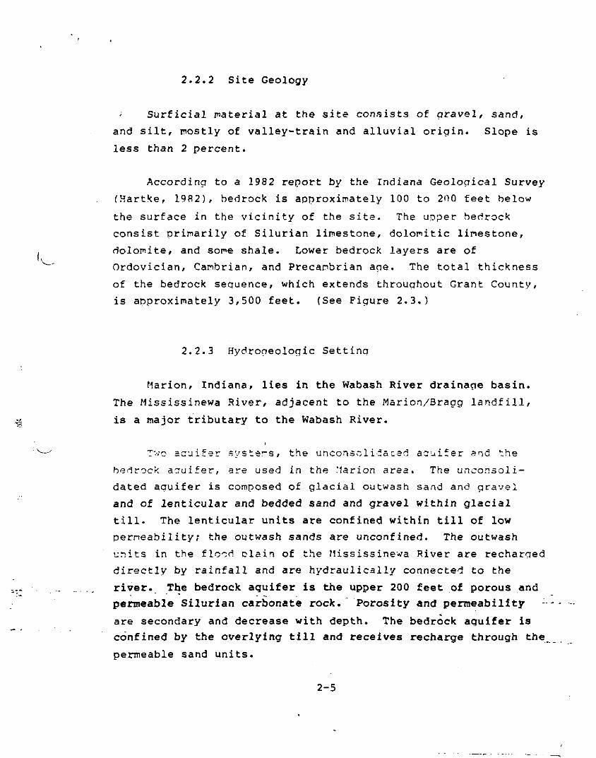
2.2,2 Site Geology

- Surficial riaterial at the site consists of gravel, sand,and silt, mostly of valley-train and alluvial origin. Slope isless than 2 percent.

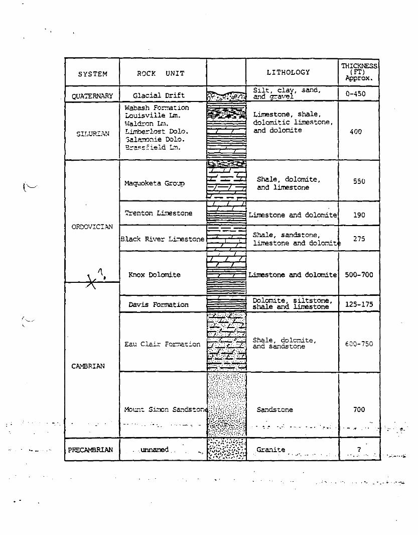
According to a 1982 report by the Indiana Geological Survey(Hartke, 1982), bedrock is approximately 100 to 200 feet belowthe surface in the vicinity of the site. The uoper bedrockconsist primarily of Silurian limestone, dolomitic limestone,dolomite, and some shale. Lower bedrock layers are ofOrdovician, Cambrian, and Precanbrian ape. The total thicknessof the bedrock sequence, which extends throughout Grant County,is approximately 3,500 feet. (See Figure 2.3.)

2.2.3 Hydrogeologic Settinq

Marion, Indiana, lies in the Wabash River drainage basin.The Mississinewa River, adjacent to the Marion/Bragg landfill,is a major tributary to the Wabash River.

iTwo acuifer systems, the unconsolidacad acuifer and the

bedrock aauifer, are used in the Marion area. The uncor.soli-dated aguifer is composed of glacial outwash sand and graveland of lenticular and bedded sand and gravel within glacialtill. The lenticular units are confined within till of lowpermeability; the outwash sands are unconfined. The outwashunits in the flood clain of the Mississinewa River are rechargeddirectly by rainfall and are hydraulically connected to theriver. The bedrock aquifer is the upper 200 feet of porous andpermeable Silurian carbonate rock. Porosity and permeability :

are secondary and decrease with depth. The bedrock aguifer isconfined by the overlying till and receives recharge through thepermeable sand units.

2-5

Fiaure 2.3. Generalized geologic section,Marion-Bragg Landfill-

2-6

SYSTEM

QUATERNARY

SILURIAN

ORDOVICIAN

CAMBRIAN

PRECAMBRIAN

ROCK UNIT

Glacial DriftWabash FormationLouisville Lm.Waldron Lm.Limbe^lost Dolo.Galamonie Dolo.

Maquoketa Group

Trenton Limestone

Black River Limestone

Knox Dolomite

Davis Formation

Eau Clair Formation

Mount Sincr. Sancston*

. -unnamed. .

?̂!5̂^SSS— * ——— * ——

' •> ' f

^^£££?

^=•5i i i

/ i

^— —— ——• , i^ ••—_\ »

/ // / /

/ /

SfeMWSf*£;£££rr^..*.-'~rr:-?r.v:"i>;.:::-'̂ V:>?:-:

jl-®:->i':^K:]

• :•••'.'.;.•.•:••.'."•.•.

'" i»V'«l^~*'™ '*•* •*.'"*'

^53^

LITHOLOGY

Silt, clay, sand,and gravel

Limestone, shale,dolomitic limestone.and dolomite

Shale, dolomite,and limestone

Limestone and dolomite

Shale, sandstone,limestone and dolomit

Limestone and dolomite

Dolomite, siltstone,shale and 1 imastone

Shale , dolomite ,anci sandstone

Sandstone

. Granite

THICKNESS(FT)

Approx,

0-450

400

550

190

275

500-700

125-175

600-750

700

• ~ -T . ' " •

7

2.2.4 Site Geohydrology

According to information currently available (Hartke,1982), at least two aquifers are located beneath the site.The shallow aquifer is unconfined. When the three existingnonitorinq wells were drilled in June 1982, the shallow aquiferwas encountered beneath 17.5 to 35.8 feet of sand and gravel.(Refuse naterials were encountered to a depth of about 25 feetin one borinp.) A deep aauifer is believed to exist in theupper 200 feet of bedrock (Indiana Geoloqical Survey, 1982).The city of Marion obtains its drinking water fron a tributaryof the subsurface Teays Valley aquifer system.

2-7

3.0 METHODOLOGY

3.1 Study Objectives

In discussions with the project officers and the Region 5technical support staff, the following objectives forgeophysical surveys at the Marion site were aoreed upon:

0 Determine the location of drun burial areas within thelandfill.

° Determine the lateral and vertical extent of thelandfill.

0 Obtain data on the shallow stratigraphy and structure.

0 Familiarize Reoion 5 technical support staff withequipment and with Lockheed-EMSCO's field methodsand procedures.

3.2 Geophysical Methods

To peet these objectives, several geophysical methods wereused (see Table 3.1). These methods include magnetics, electro-magnetic induction, seismic refraction and resistivity.

*

3.2.1 Magnetics

The magnetic method measures the total intensity of theearth's magnetic field* The method uses the precession of . '"-spinning hydrogen protons inA*fa%*r to measure total magneticintensity." When "a magnetic field is applied, the spinningprotons become temporarily aligned. When the magnetic field is

3-1

TABLE 3.1. METHODS USED AND RATIONALE FOR GEOPHYSICAL SURVEYS

___ AT THE MARION fBRAGG) LANDFILL___________

Objective Method Rationale

1. Locate buriedr'runs and petal

Electro-magnetics(EM31)

The EM31 meter measuresthe conductivity of theearth to a depth ofapproximately 12 feet.This method is used tolocate and delineateconductivity highs/ suchas are caused by thepresence of netal, andto determine the orien-tation of those hiohs.

Maanetics The Geometries protonprecession magnetoneter/^radiometer measures thetotal magnetic field andthe Gradient of thatfield. It can be usedto locate ferrousobjects, such as drumsor car bodies.

2. Determine lateral Electro-and vertical extent magneticsof landfill. (EM31)

These instruments canbe used to measure theconductivity of theground to determine thelateral extent of thefill.

(continued)

3-2

TABLE 3,1 (continued)

' Objective Method Rationale

Resistivitysounding

The Bison resistivityunit with the BOSSsystem can be used to<*o resistivity soundingsto trv to determine thedepth of the fill.

3. Obtain data onshallowstratigraphyand structure.

Resistivitysoundina

Offsite and onsitssoundings are used todetermine the verticaldistribution of r~</Xmaterials and depth tothe water table.

Seismicrefraction

This method, using theBison Geopro seismicsystem, is used toobtain complernentaryacoustic data enstratigraphy andstructure.

4. Familiarize EPApersonnel withecuiprent, methods,and procedures.

All methods Future EPA studiesrequire that EPA Region5 personnel work withthe Lockheed-SMSCO teamduring the siteinvestigation to becomefamiliar with eauipraentand procedures.

3-3

removed, the protons•precess about the direction of the earth'smagnetic field. This produces a small sianal whose freauencv isproportional to the earth's magnetic field.

A larcje iron object will produce a nore intense anomaly thanwill a small iron object buried at the sane depth. An objectburied at shallow depth will produce a nore intense anonaly thanwill the sane object buried deeper.

Transformers, Power lines, fences, and other electrical andmagnetic objects may cause interference with the magnetometerreadings.

3.2.2 Electromagnetic Induction

Electromagnetic induction (EM) measures soil electricalconductivity. An oscillating electromagnetic field istransmitted from, a circular transmitting coil, which induceselectrical currents in the ground. Fields created by thesecurrents are detected by a separate receiving coil. Thetransnittina and receiving coils are separated by a specific•ristancs. I r. cress i": 7 the separation of the coils increases the

of exploration.

EM induction surveys can also be used to locate localanomalies in soil conductivity. Anomalies may be responses toburied metallic objects, contaminant plumes, or other localizedcultural or ceolorjic features that affect soil conductivity.Cultural features such as underground conductors (for example,large pipes) are easily recognized by large meter fluctuationsthat occur within short distances. Fences, overhead power lines,and other nearby metallic objects may also influence readings.Geologic features, such as lateral or vertical inhoroogeneities insoils that have different conductivities, can also be detected.

3-4

Sone limitations need to be considered when interpreting EMdata. Some contaninant plumes are easily detected using EMinstruments, but only when the contaminants cause a change inconductivity. Without a conductivity change, a contaminant plumeis not detectable with EM techniques.

3.2.3 Resistivity

The resistivity method measures the electrical resistivityof the soil. An electric current is passed into the around froma pair of electrodes, and the electrical voltage is sensed by asecond pair of electrodes. Resistivity data are generallyrecorded as apparent resistivity, pa, which can be found from:

pa = K 9 -

where K is the geometric factor, V is the observed voltage, and Iis the injected current. K is a function of the geometry of theelectrodes (called an array). The basic unit of neasors ofresistivity and apparent resistivity is the ohm-meter.

The Henner arrav is the most commonly used array forhydrological studies• The major advantages of this array arethat it has a nuch lower sensitivity to geologic noise and tolocalized changes in soil resistivity unrelated to large-scalefeatures of interest, and it returns a relatively hicrh voltagefor a small transmitter current; thus, small transmitters nay.beused. Its major drawbacks lie in having sore./hat lower verticalresolution and much lower horizontal resolution than some otherarrays. For the Wenner array, the geometric factor is given by:

pa * 2va.

3-5

The apparent resistivity is not indicative of the resistiv-ity at any single depth, but is an average of soil resistivityover a range of depths. The depth of exploration is proportionalto the a-spacing used; the dominant response usually cones from adepth of about one-third to one-half of the a-spacing. Soundingsare taken by making a series of measurements starting with shorta-spacinn (less than 1 m) and increasing the spacings loaarithni-cally to several tens or hundreds of neters.

Sediments and near-surface rocks that contain little or noclay usually exhibit low resistivity. Conduction of electricityin these rocks is alnost entirely through the movement of ions inthe fluids within the pore spaces. Very little current istransmitted through most mineral grains. Therefore, the greaterthe concentration of ions, and the greater the porosity, thelower the bulk resistivity of the sediments, the relationbetween porosity, fluid conductivity, and bulk resistivity, p, ofsediments is given by Archie's Law:

m A ̂P = <£ 0 ̂ $ ——

*> <f

.-.ssu"i?.c that all of the oore soace is filled with fluid, $ isthe oorosity of the sediments and n is the coefficient oftortuosity. In this equation, a is the conductivity of the porefluids. Most ground waters have conductivities ranging from 0,1to 0.01 Siemens per meter [S/m (1 S/m = 10,000 micromhos/cm)],but the conductivities of brines nay exceed 5 S/n. Althoughconductivity of water varies somewhat with the particular ionspresent and the t=rp era tare cf cne .vacer, a roach a.^oroxirstio-for ground-water conductivity is given by:

a<s/m) * TDS fmg/L)7,000

where TDS is total dissovled solids.3-6

This representation accounts for the irregular path that thecurrent nust follow through the soil; the more tortuous thecurrent path the higher the value of m. For different soil androck types in varies from 1.3 to 2.0, but a value of 1.5 givesaood results for most surface alluviun.

3.2.4 Seisnic Refraction

The seismic refraction method is based on the assumptionsthat (1) layer acoustic velocities increase with depth,(2) sufficient contrast exists between velocities, and (3) layersare thick enough to permit detection. The technique can be usedto define nany natural and geohydrologic conditions includingnunber and thickness of layers, layer composition and physicalproperties, depth to bedrock or water table, and anomalousfeatures.

Primary conpressional waves move through subsurface geologiclayers in response to layer physical properties, thickness, andsequence, A significant change in any one of these paraneterswill cause a notable shift in wave velocity and path of travel.Seisric refraction is used to detect these shifts.

Acoustic velocity in the layer is determined prir.arily bythe density and the elastic properties of the layer. In turn,density and elasticity are affected by the porosity, mineralcomposition, and v/stsr content of the layer.

Two or rore aeolocic layers ^ay be resolved usinr: thefj

seisnic techigue. A seismic source produces sound waves whichtravel in all directions into the ground. One of these wavesr

the direct wave, travels parallel to the ground's surface, withinthe surface layer. A seismic sensor (geophone) detects thedirect wave as it moves along the surface layer. The time of

3-7

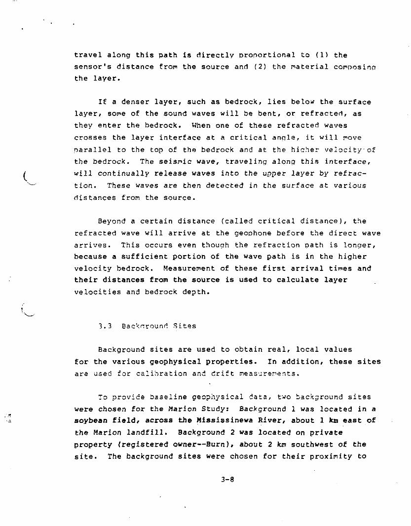
travel along this path is directly proportional to (1) thesensor's distance from the source and (2) the material composinathe layer.

If a denser layeri such as bedrock, lies below the surfacelayer, some of the sound waves will be bent, or refracted, asthey enter the bedrock. When one of these refracted wavescrosses the layer interface at a critical angle, it will moveparallel to the top of the bedrock and at the higher velocity ofthe bedrock. The seismic wave, traveling along this interface,will continually release waves into the upper layer by refrac-tion. These waves are then detected in the surface at variousdistances from the source.

Beyond a certain distance (called critical distance), therefracted wave will arrive at the geophone before the direct wavearrives. This occurs even though the refraction path is longer,because a sufficient portion of the wave path is in the highervelocity bedrock. Measurement of these first arrival times andtheir distances from the source is used to calculate layervelocities and bedrock depth.

3.3 Background Sites

Background sites are used to obtain real, local valuesfor the various geophysical properties. In addition, these sitesare used for calibration and drift measurements•

To provide baseline geophysical data, two background siteswere chosen for the Marion Study: Background 1 was located in asoybean field, across the Mississinewa River, about 1 km east ofthe Marion landfill. Background 2 was located on privateproperty (registered owner—Burn), about 2 km southwest of thesite. The background sites were chosen for their proximity to

3-8

the landfill, the lack of cultural interferences, and theiraccessibility. The opportunity to return daily to a reasonablyculture-free site increases confidence in the stability of theinstruments and the measurements.

3-9

4.0 RESULTS

4.1 Magnetics

To locate concentrations of drums, magnetic data were takenusing a Geometries proton precession magnetometer. Because thelandfill had a high metal content, very little sophisticatedorocessinp was done on the magnetometer data. The laroe arealextent and the high magnetic Gradients mak^e. this data setdifficult to manipulate. Figure 4.T̂ shows 'the magnetic data set

(^ ' *?~^ ^ ' "*** ̂, for all values over 54', 5 00 gawmas, "(the. background value).. The,.^,V ~ 1-6- 'e ** '$«•*""' -2. * '' *~' A/lK-A»<" -g i<4. p.'i+ff- ,3tjr,'_*A ^~

.03:-' ' ranpe over the site was from 51,000 ganma^s near the lake to over63,000 gammas along the southern east-west road (baseline area).

The areas of highest values are clearly visible in Figure4.2. On the northern side of the site there are two elongatedareas, the northernmost area, M-l {magnetic anomaly - i^area 1),runs along lines 17+OON, 16+50N, and 16+OON from 1+OQE to 9+OOW.The second area, M-7, lies just south of M-l', along lines 14+OONand 14+50 from 9+OOU to 1+OOE, On the southeast side of thelandfill, two other areas have concentrations of high magneticvalues. Area M-3 is primarily along line 4+OOE from 6+OON to12+OOM, with sere areas cf line 5+00£ included. The largest areawith the hiqhest values, designated M-4, lies between lines 3+50Nand 0+00 from 0+00 to 11+OOE. These areas coincide withanomalies identified in other data.

4.2 Electromagnetic Induction

The EM data were gathered using £ Geonics EM-31 in verticaland horizontal modes. The instrument was checked each morningand afternoon at the background site to detect drift or malfunc-tion. The results of the surveys are presented in three modes,each of which shows a different aspect of EM properties of the

4-1

Figure 4.1. Magnetic data for all values over 54,500 gammas,Marion-Bragg Landfill.

4-2

YWAX » 2100

N-

oioi

01 Ql01

01 01

01

3

a

YMIN - -950

MARION MAGNETOMETER

Figure 4.2. Magnetic data (areas of highest values),Marion-Bragg Landfill.

4-3

YMAX = 2100

\

YMIN - -950

MARION MAGNETOMETER

site. The first node, Figures 4.3 and 4.4, shows the data pointswith contours. The second node. Figures 4.5 and 4.6, shows onlyt,he averape values contoured. The contour naps show the overalldistribution of metal and conductive ground. The backgroundreadings in the area are from 3 millimhos/n to 17 millinhos/m.Inspection of the contour maps shows no indication in thesouthern annex (the area south of the east-west baseline) of anyconductive anomalies. However, in the area west of the nond andnorth of the asnhalt plant (lines 6U to 10W, 8?J to 13M), thesmall indentation of land into the pond (lines 317 and 4W from 8wto ION) appears to contain a concentration of metal. The thirdnode. Figure 4.7, shows those points where the meter went tozero; these are the points that indicate the greatest concentra-tion of metal. Three locations are seen in the northern sector:

Anomaly EM-1 (electromagnetic anomaly - area 1), stretches acrossth entire northern sector from the edge of the data near the pondto 10+0 ON. The second anomaly, EM-2, lies in the area east ofthe pond, along lines 5E and 6E from. 4+OON to 10+OON. The thirdanomaly, EM-3, runs east-west along the baseline.

Exclusive of the three zero areas, anomaly EM-4, an area ofhigh conductivity, is most significant. EM-4 lies along lines INand 2:i from 3 + OOE to 10+OOE. The E.'I data recorded for this arsarelate well to associated resistivity results.

The rest of the landfill exhibits high conductivities thatare normally associated with landfills. These levels of conduc-tivity coLilc result f rsr. the presence sf ret si iras/. , rr.-rs / o_~

/conductive fluids en fill material.

c^i'fi^v S ̂ ' ' !"1 d ̂ TT an*"' S*3!!?*̂ ^̂

Four refraction lines werex collocated with resistivityftHf»*e*A''*p.

soundings ff, 9, 10, and 15? No refraction line was run without asounding, however. Figure 4.8 shows the location of the

4-4

Figure 4.3. EM properties, mode one (vertical)

4-5

YMAX - 2100

D1 Q1 Q1 Ql O!O1 Q1 01 O1

Ql Ql1 Ql Ql Ql

ol at ai01 Q1 Ql01 at QI oiat ai 01 at

ai aioiQl Dlat atat01 ai

MARION EM31 VERTICALYWN * -950

AVERAGE

Figure 4.4. EM properties, mode one (horizontal

\Tt4AX * 2100

at a a^al aif» 01 01 al ai

ai ai aiai

aiQl

Ql Dl Qlai ai QI

YWN - -950

MARION EM31 HORIZONTAL AVERAGE

Figure 4.5. EM properties, mode two (vertical)

4-7

WAX = 2100

MARION EM31 VERTICAL\VtlN '

AVERAGE-950

Figure 4.6. EM properties, mode two (horizontal).

4-8

= 21OO

MARION EM31 HORIZONTALYMN - -950

AVERAGE

Figure 4.7. EM properties, mode three (vertical)

4-9

YMAX s= 2100

Dl DlDlDl 01

01 DlDl Dl

01ni al

Q1Q1 Q1

1 Dl Dl1 Dl Dl Olpi DI

B1 DI ai

Dl

Ql

Dlai

01ai

Dl

YMIN - -950

MARION EM31 VERTICAL LESS THAN ZERO LOCATIONS

resistivity soundings and the orientation of the array. Table4.1 shows the resistivity soundinp data.

T?VBLE 4.1. RESISTIVITY SOUNDING DATA

Soundina Location Layer1 Backoround Site 2 1

7.3

2 5+OOE, 8 + OON

3 Background Site 1 12

34

4 7+4QW, 11+OON5 9-r50E, 3+C03 1

(southern annex) 2

6 3+OOU, 15+OON 123d

7 6+OOE, 3+OON 123a.5

8 10+OOE, 6+OOS 1(Southern Annex) 2

34

AnparentResistivity

79 £•>•*5592P

unnodelable

4724672336

no data23

218

592445159

49132.3

49

2,050

469258240

Depth02.58.5

-

00.966.4

33

-

06.5

0

0.392.615.6

00.94171927

00.352.619

InterpretedMaterial

surface claysand/waterclay

-

surface claysand/waterclaysand/water

-claysand/water

surfacefill 'claywatarsurfacefillfillclaysand/gravel

surfaceclay/sandclaywater

(continued)4-10

TABLE 4.1 (continued)

Soundino Location Layer9 5+OOW, 16+OON 1

234

5

10 6+OOE, 7+50N 12345

11 7+0017, 16+OON 123

12 4 + 0017, 16 + OON 1

23

13 1 + 0057, 15 + 50N

14 2+OOE, 3+25N 1

2

3.15 6+50E, 5+OON 1

23A

ApparentResistivity

133 -&•*813451135

1002293

90725

803017

1273667

unnodelable

612112764

143

1337

Depth

00.671.5

7.5

30

00.331.94.812

0117

01.54.2

01.3

3200.71.49

InterpretedMaterialsurfacefillfillclay

surfacefillfillclaysand/water

surfacefill/clay?water

surfacefillclay

-

surfacefillwatersurfacefillfillclav?

4-11

Figure 4.8. Resistivity sounding locations

4-12

'MARION LANDFILL RESISTIVITY SOUNDING LOCATIONS1

Sounding 2 was centered at 5+OOE, 8+OON running north-south.The data were judqed unmodelable owing to high observationalefror and lateral inhomoqeneities. The sounding curve was toocomplex to be modeled, probably because of the highly variablenature of the fill material at that location.

Sounding 4 was not completed owinn to extremely high-stakeinpedences. The resistivity unit at hand could not operatewithin its range at the sounding 4 location.

Soundinq 5 was located in the area south of the east-westbase (the southern annex). It was centered on 9-t-SOE, 3+OOS, andran northwest-southeast. The model was arrived at by inversemodeling, resulting in a reasonable fit to the data. At thislocation there appears to be a conductive clay layer to a depthof about 6,5 m, beneath which is the water table.

Sounding 6 was centered at S^OOH, 15+OON with the arrayoriented east-west. The scatter in the data was so great thatinverse modeling did not yield a satisfactory result. Therefore,the model was arrived at through successive forward rcodels. Thesounding is not a good fit; however, it is the best presentlyattainable. The nodel has three successive layers of lowresistivity. The first two are interpreted as landfill, thethird is probably an underlying clay; the water table is at adepth of about 16 m,

Soundinq 7 was centered at 6+QOE, 3+00:?, with the arrayoriented east-west. The scatter in the data made an inversion byin-house software impossible, so a node! was arrived at bysuccessive forward models. Fit to the r.ccel is net particularlygood beyond the first and second layers. There appears to be alayer of 13-r-n material about 16 n thick overlying a 2-m thick,very low resistivity layer. Beneath this layer appears to beclay overlying a resistive layer. The values for layers 3 and 5

4-13

o£ 2.8 r-m and 2r050 r-m respectively are not accurate. Theyshould be regarded as order of magnitude values rather than ase^act resistivities.

Sounding 8 was centered at 10+OOE, 6+OOS, with the arrayoriented north-south. The model was arrived at using successiveforward models to fit the data. The model consists of fourlayers, the first three are primarily clay, with some sand in thesecond layer, bringing the apparent resistivity up a bit (92 asopposed to 40 to 55). The data indicate a water table at 19 m.Seismic refraction was also run on this line. These data indi-cate three acoustic layers (see Table 4.2). The first layer isl',850 ft./sec.', indicating a loose, dry surface layer about 5 to7 feet thick. The second is a 4,500 ft./sec. layer that couldindicate clayey sand or a water table. This layer is 10 to 15feet thick. The third layer is 7,400 ft./sec., most probablyindicating a competent clay. This layer is of indeterminablethickness.

TABLE 4.2. SEISMIC REFRACTION DATA______________

RefractionLine

BG-1

ResistivityLineBG-1

LayerVelocityfc./sec.

InterpretedMaterial

V

1600 Surface material5600 Water

15 1100 Fill

2*

3G-2

123

12

185045.107400

12006500

Surface materialClayey sancl-'watsClay

4* 1150 Fill

5* 104-14

1150 Fill

Sounding 9 was centered on 5+OOW, 16+OON, with the arrayoriented east-west. The final model was achieved by successiveinterations using a forward model. There is considerable scatterin the first two layers; however, the lower layers modeledreasonably well. The model shows three layers of landfillmaterial overlying a clay layer (51 r-m) about 7.5 m deep. Thisclay layer in turn overlies a more resistive layer. The depth toclay is believable; however/ 30 m to the water table may not bereal. A seismic refraction line was collocated with thissounding. The results show a layer of 1,150 ft./sec. materialabove 6 to 8 m, with no indication of a more dense layer below.Deeper penetration was impossible due to the attenuation effectsof the fill material on the acoustic signal.

Sounding 10 was centered on 6+OOE, 7+50N, and the array wasoriented north-south. The data were scattered and not modelableby inversion. A model was arrived at by forward modeling. It isnot a good fit, but it does give a general indication of subsur-face. There is a very conductive layer at least 3 m thick thatis overlain by two thin resistive (dry and sandy) surface layers.Beneath the conductive layer is a 90-r-n layer, probably a sandyclay, and at about 12 m is the water table. The fit to thesedata is not good, but this model is consistent if not precise.

SouncHno 11 was located at 7+OOU, 16+OON, and the array wasoriented north-south. The model was constructed using thein-house R3INV program. The data are scattered and the fit isnot rroocf. The pocel indicates that the fill layer is about 15 ~thick overlying the water table. This estimation is probably toodeep. The 30-r-n layer could be an unresolved mixture of filland clay or two distinct layers with little resistive contrast.Fill thickness at this site cannot be determined. Seisnicrefraction was attempted at this sounding, but background noiseprevented the collection of data.

4-15

Sounding 12 was located at 4+OOW, 16+OON, with the arrayoriented north-south. The model was obtained by inversion withthe R3INV program. The curve fit is good in the upper layers.Data appear a bit scattered in the conductive layer, and theprogram statistics indicate that the thickness of the secondlayer is only moderately precise. However, the model does allowan estimation of the fill thickness and a determination of thebottom layer material. The fill is about 4 m thick and appearsto be over a clay.

Sounding 13 was centered on 1+OOW, 15+50N, and the array wasoriented north-south. The data appear to indicate alternatinglayers of conductive and resistive layers. The scatter in thedata is due to the large difference between the two offset Wennerarrays, DI and D2- This offset error renders the dataunmodelable.

Sounding 14 was centered at 2+OOE, 3+25N, and the array wasoriented east-west. The inverse model was developed using theR3INV program. The overall fit is good; however, the apparentresistivity of the last layer is unresolved according to theprogram statistics. However, the curve fit is good enough tolend confidence in the magnitude of the value, if not in theprecision. The model shows a thickness of fill of approximately30 m. This seens deep in light of the site history; however, itis consistent with sounding 7. The thickness of fill was 19 mand the water table was at 27 m. This area shows both magneticaruj electromagnetic anonalie* ; the so ret hods indicate anelongated structure of some depth.

Sounding 15 was centered on 6+59E, 5-»-00.>:, and the array wasoriented east-west. The model was obtained by inversion. Thefit of the model to the data is reasonable for the first andthird layers. The second layer resistivity and thickness are notresolved. The resistivity of the fourth layer does not appear

4-16

(from the curve) to be high enouqh. With these caveats, themodel indicates three layers of fill to a depth of about 9 m.Below the third layer, which is quite conductive, a clay layermay be present.

4-17

5.0 CONCLUSIONS

5.1 Summary of Data

The field phase of the Marion landfill study ran for 3 weeksduring autumn 1985. During that period, geophysical data weregathered by personnel from EPA Region 5, R. F. Weston, andLockheed-EMSCO. Table 5.1 summarizes the tally of field data bymethod.

TABLE 5.1. SUMMARY OF FIELD WORK

_____Method___________Quantity______EM-31 5 kmMagnetics 5 kmResistivity soundings 15Seismic refraction 4 120-ft spreads

5.2 Landfill Structure

The Marion landfill is located in a former gravel miningarea. As such, the thickness of the fill material can be expectedto vary over the extent of the site. Figure 5.1 is an isopach mapof fill thickness using the resistivity data and visualobservation.

5.3. Objectives

Table 5-2 lists the objectives and the results of the Marionlandfill study. Most cf the objectives were net. Several areas,designated M-I, M-2, M-3, EM-1', and EM-2, were identified ascoincident anomalies, indicating a high concentration of metal.The linear magnetic anomaly in the vicinity of lines IN, 2N, and3N, coupled with the high conductivity of the area, indicates aprime target area. The resistivity shows a very thick layer offill. These factors may indicate that a trench yg present.

A*y

s-i

Figure 5.1. Isopach nap of fill thickness5-2

"ISOPACH MAP OF FILL'

LEGEND(17) THICKNESS OF

FILL IN METERS

,5 RESISTIVITY«i±» SOUNDING

LOCATION

CONTOUR INTERVAL5 METERS

TABLE 5.2. STUDY OBJECTIVES WITH RESULTS

Objective Result1* Determine the location

of drum burial areaswithin the landfill.

Several areas of coincident magneticand electromagnetic anomalies wereidentified. However, the landfill ingeneral appears to contain a highpercentage of metal trash.

2. Determine the lateraland vertical extentof the landfill.

3. Obtain data on theshallow stratigraphyand structure.

4. Familiarize the EPA-Region 5 technicalsupport staff withLockheed-EMSCO's fieldmethods and procedures

The boundaries of the landfill andcertain nonfill areas were identi-fied. An isopach of fill thicknesswas constructed (Figure 5.1).

Both background site data sets wereof good quality. Depth to clay anddepth to water were determined. Lackof an integrated map and detailedtopography data make further analysisimpossible.

Region 5 staff performed most of thedata collection and field setup andhave worked closely with theLockheed-EMSCO technical lead.

The lateral extent of the landfill is indicated byelectromagnetic readings between 10 and 30 over a wide area. Twosuch areas exist within the study area, the southern annex(portion of the site south of the east-west baseline), and thearea between the lake and the cemetery (except the elevatedportion adjacent to and jutting into the lake). The perimeter ofthe fill is generally marked by an old tree line. The verticalextent of the landfill is shown on Figure 5.1. More detailed maps

5-3

'MARION LANDPf&OPftCBIBXPVOFVFICCUNDING LOCATIONS'

(17) THICKNESS OFFILL IN METERS

RESISTIVITYSOUNDINGLOCATION

CONTOUR INTERVAL5 METERS

of the strata below the fill cannot be constructed until atopographic map of the site is completed.

The shallow stratigraphy of the background sites is describedin the results section. Further interpretation of site structure,and construction of table maps will be possible only after atopographic map is constructed and detailed test boring logs areavailable. As was expected/ the stratigraphy of the fill appearsto be highly variable. In general, a thin clay layer containingsome sand and fill overlies a conductive layer of fill of varyingthickness and composition. The base of the fill varies between aconductive clay layer and a resistive sand/water layer.

To assure adequate procedure familiarization, the EPA Region5 technical support staff used their own equipment to collectfield data. In most instances, they collected data and entered itinto the computer or onto the contour maps with only occasionaladvice from the Lockheed-EMSCO team. Although analysis andreporting were performed by Lockheed-EMSCO, the Region 5 staffhave remained in contact with the technical lead and have receivedsupport for subsequent data analyses. This is the final CERCLASite Report of the Lockheed-EMSCO Geophysical Field OperationsSection.

5-4