University of KentuckyUKnowledge

KWRRI Research Reports Kentucky Water Resources Research Institute

8-1972

Location of Solution Channels and Sinkholes atDam Sites and Backwater Areas by SeismicMethods: Part IDigital Object Identifier: https://doi.org/10.13023/kwrri.rr.54

Vincent P. DrnevichUniversity of Kentucky

S. R. SmithUniversity of Kentucky

E. P. ClevelandUniversity of Kentucky

Right click to open a feedback form in a new tab to let us know how this document benefits you.

Follow this and additional works at: https://uknowledge.uky.edu/kwrri_reports

Part of the Geophysics and Seismology Commons, Soil Science Commons, and the WaterResource Management Commons

This Report is brought to you for free and open access by the Kentucky Water Resources Research Institute at UKnowledge. It has been accepted forinclusion in KWRRI Research Reports by an authorized administrator of UKnowledge. For more information, please contactUKnowledge@lsv.uky.edu.

Repository CitationDrnevich, Vincent P.; Smith, S. R.; and Cleveland, E. P., "Location of Solution Channels and Sinkholes at Dam Sites and BackwaterAreas by Seismic Methods: Part I" (1972). KWRRI Research Reports. 141.https://uknowledge.uky.edu/kwrri_reports/141

Research Report No. 54 University of Kentucky Soil Mechanics Series No. 14

Location of Solution Channels and Sinkholes at Dam Sites and Backwater Areas by Seismic

Methods: Part I Rock Surface Profiling

Dr. Vincent P. Drnevich Principal Investigator

Graduate Assistants: S. R. Smith E. P. Cleveland

This is Part I of a two part final completion report. Part II is entitled, "Correlation of Seismic Data with Engineering Properties," and has been issued as Water Resources Research Report No. 55.

Project No. A-026-KY (Partial Completion Report) Agreement Number 14- 31-0001-3217 (FY 1970)

Period of ProJect: Sept. 1970 - June 1972

University of Kentucky Water Resources Institute Lexington, Kentucky

The work on which this report is based was supported in pa.rt by funds provided by the Office of Water Resources Research, United States Department of the Interior, as authorized under the Water Resources Research Act of 1964.

August, 1972

ABSTRACT

The basic concepts associated with the sledge hammer seismic refraction survey are reviewed and a modified version called down hole shooting is discussed. The latter method has distinct advan­tages for rock surface profiling. These include: calibration at the end points of the survey, measurement of vertical wave propaga­tion velocities directly, and having a refracted wave ray path for almost the entire survey length.

The down hole shooting seismic refraction survey has been simulated with the digital computer. The method can handle any shaped rock surface profile and generates corresponding travel time curves for the forward and reverse profile surveys. This pro­gram was used to systematically study the effects of anomalies on the travel time curves. A method of data reduction was developed that enables an estimate of the rock surface profile to be made from the travel time data. The procedure involves the use of a reference depth line which cmnects the end points of a survey and the travel time curves for this reference depth line.

Field tests were performed at four sites having soil and rock characteristics different from each other. Typical results are given. Rock surface profiles are estimated from the travel time curves using the procedure developed and these are compared with the depth to rock by proof drilling.

Finally, the sources of error are discussed and some limita­tions of use are presented. For the sledge hammer method to be used for rock surface profiling, the rock surface should be within 25 to 30 ft of the soil surface and the minimum width of solution channel that can be sensed with this method is on the order of two feet. Recommendations for additional research are also given.

KEY WORDS: boreholes, computer models'~, computer programs*, down hole shooting surveys*, exploration, geophysics, on site investigations, rocks, rock surface profiles'', seismic properties, seismic refraction surveys'', seismic studies, seismic waves'", seismographs*, seismology, soil dynamics, soils, subsurface mapping--:<, travel times.

ii

ACKNOWLEDGMENTS

The research reported herein was sponsored by the Office of

Water Resources Research, Project A-026-KY. The author

gratefully acknowledges this support. He also wishes to thank

his colleague, B. 0. Hardin, for his helpful suggestions, graduate

students E. P. Cleveland, D. Raghu, and S. R. Smith for their

efforts and contributions, and undergraduates C. S. Bishop and

R. H. Stith for their assistance,

Several local consulting engineers have been most helpful. In

particular the author wishes to thank John Stokley of Stokley and

Associates and Louis Snedden of Mason & Hanger - Silas Mason Co,

for their interest.

Finally the author wishes to thank the U. S. Army Corps of

Engineers, Louisville District and Charles Ballman, Lockmaster,

Lock 9, for their cooperation and access to the site.

iii

TABLE OF CONTENTS

List of Figures v

Chapter I Introduction 1

Chapter II Research Procedures 4

Standard Seismic Refraction Method 4 Down Hole Shooting Method 8 Seismic Refraction Equipment 10 Computer Simulation of Seismic Surveys 11

Chapter III Data and Results 13

Computer Generated Travel Time Curves 13 Generalized Procedures for Rock Surface Profiling 15 Description of Field Test Sites 20 Typical Field Travel Time Curves 24 Methods of Checking Rock Surface Profiles 27 Comparison of Predicted and Measured Rock

Surface Profiles 27 Comparison of Predicted and Measured Travel

Time Curves 28 Discussion of Errors and Limitations of Use 29

Chapter IV Conclusions 35

References 37

Appendix I Notations 38

Appendix II Seismic Refraction Simulation Program 40

iv

LIST OF FIGURES

1. Standard Seismic Refraction Survey 5

2. Seismic Refraction Survey Method for Interpreting between Boreholes 9

3. University of Kentucky Seismic Refraction Survey Equipment 12

4. Typical Computer Generated Travel Time Curve 14

5. Travel Time Curves for Reference Depth Line 16

6. Intercepts for Reference Depth Travel Time Curves 18

7. Slopes for Reference Depth Travel Time Curves 18

8. Horizontal Distance Correction 19

9. Procedure for Estimating the Depth of Channel 21

1 o. Corrections for Reference Depth Travel Time Curve Due to Channel 22

11. Procedure for Determining Height of Hump 23

12. Travel Time Curve and Data Reduction at Campus Site 25

13. (a) Field and Computer Generated Travel Time Curves 26

(b) Predicted and Observed Rock Surface Profiles 26

14. Minimum Normalized Channel Widths for First Arrival Ray Path Around Channel 34

v

CHAPTER I

INTRODUCTION

The main objective of this project was to adapt the methods

of seismic refraction surveying to the accurate determination of

depth and undulation of the rock surface where the depth tci rock

is less than 50 feet, This research was aimed particularly at

locating solution channels and sinkholes in the limestone beneath

the usually shall ow overburden that exists at potential dam sites

and back water areas.

Kentucky and a number of other states have significant

limestone deposits. Limestone dissolves when slightly acid

ground water comes in contact with it. The process is termed

solutioning. Unique features develop when the solutioning process

has been active in an area. The resulting caves, sinkholes, and

solution channels present problems for practically all development

and construction. These problems can be especially important

where water retention or water distribution systems are built.

For example, a gigantic solution channel had to be sealed off with

a combination of cutoff walls and grouting before Kentucky Dam

in the western part of the state could be constructed (1).

One of the first methods that should be used to determine

whether the problem exists at a site is to review the geology and

geologic history of the site. Bishop (2) has reviewed the geology

and physiography of Kentucky with emphasis on the zone that con­

trols most engineered projects. He also reviewed the process of

solutioning and described the development and nature of solutioning

1

for different geologic conditions. Solution features may be on the

surface of the bedrock (solution channels) or wholly within the

limestone (caves and caverns). Occasionally, caves or caverns

may have nearly vertical openings to the surface. These are

termed sinkholes or sinks.

The soils overlying the limestone in Kentucky are generally

residual and are usually less than 10 feet in thickness (2). Solution

features may or may not be expressed by the surface topography

depending on the thickness of soil, erosional history and nature

of the solution features. For example, surface topography would

not be affected by caverns or by very small solution channels and

sinks.

At present there are no economical and foolproof methods

to locate solution features. To locate caves and caverns, time

consuming and expensive drilling is used. This is often unreliable

because the features may be relatively small compared to the drill

spacing. To locate sink holes and solution channels, both auger

borings and soundings are used. However, many are never found

or are found when the excavations for the facility are made.

Several aspects related to the existence of solution channels

and sink holes suggested that seismic methods might be favorably

used for their detection and description. These aspects include:

1) relatively shallow soil cover, 2) relatively uniform soil pro­

perties, and 3) sharp contrast between soil properties and rock

properties. A review of previous efforts in this direction was made

by Anderson and Girdler (3). This report is concerned with the

development of the procedure to determine the rock surface profile

by seismic methods. The method of approach was to simulate the

seismic refraction survey with the digital computer and then to

systematically vary the characteristics of the profile. The

2

resulting data were used along with the principles of wave propa­

gation to develop a semi-empirical method for locating and sizing

anomalies such as solution channels and sinkholes. In addition,

field surveys were performed. The data were used to predict

rock surface profiles. Proof drilling and sounding were used to

establish the actual profiles so that comparisons could be made.

In addition to describing the above research, this report will also

discuss some of the sources of error and limitations of the seismic

refraction method for rock surface profiling.

3

CHAPTER II

RESEARCH PROCEDURES

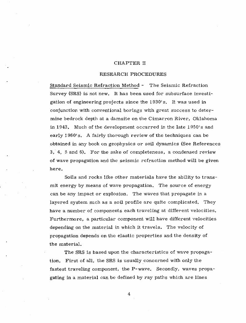
Standard Seismic Refraction Method - The Seismic Refraction

Survey (SRS) is not new. It has been used for subsurface investi­

gation of engineering projects since the 19301 s. It was used in

conjunction with conventional borings with great success to deter­

mine bedrock depth at a damsite on the Cimarron River, Oklahoma

in 1943. Much of the development occurred in the late 1950's and

early 19601 s. A fairly thorough review of the techniques can be

obtained in any book on geophysics or soil dynamics (See References

3, · 4, 5 and 6). For the sake of completeness, a condensed review

of wave propagation and the seismic refraction method will be given

here.

Soils and rocks like other materials have the ability to trans­

mit energy by means of wave propagation. The source of energy

can be any impact or explosion. The waves that propagate in a

layered system such as a soil profile are quite complicated. They

have a number of components each traveling at different velocities.

Furthermore, a particular component will have different velocities

depending on the material in which it travels. The velocity of

propagation depends on the elastic properties and the density of

the material.

The SRS is based upon the characteristics of wave propaga­

tion. First of all, the SRS is usually concerned with only the

fastest traveling component, the P-wave. Secondly, waves propa­

gating in a material can be defined by ray paths which are lines

4

"'

d.l E i-d) > ~

t= 2H~ 1-(:~)2 V1 V2

------

1

I t I t I I t I I

1

: Distance from Geophone I

Geopho7.A

q : t i ! F

x I .,,rSource Points~ d1/I. 1B \~

I I I

I I I I

Layer 1 (soil) Vel. = v1

E D C Layer 2 (rock) Vel.= v2

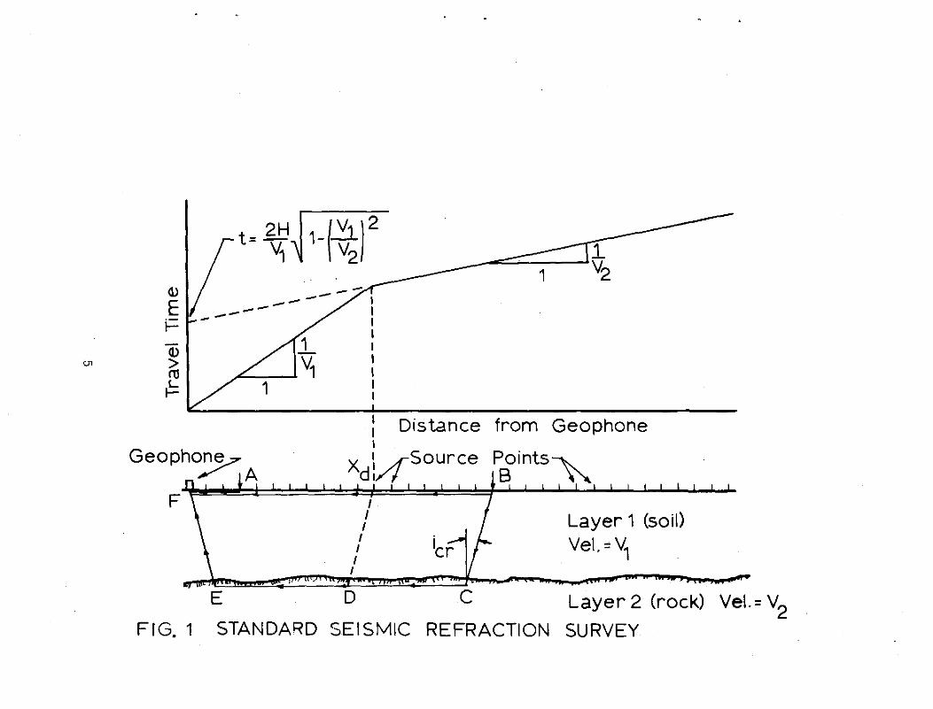
FIG. 1 STANDARD SEISMIC REFRACTION SURVEY

describing the advancing waves. In general, a wave has an infinite

number of ray paths but for a SRS, we are only concerned about

two of them, the direct ray path and refracted wave ray path. The

direct ray is one that goes from the source to a point in the same

material by the shortest means, a straight line. The ray path from

point A in Fig. 1 to the geophone is a direct ray path. As a wave

in one layer impinges on another layer the ray path is refracted

or bent. The amount of bending depends on the angle of incidence

and on the ratio of the wave propagation velocities in the two

materials. Snell's law describes refraction and it is given by:

=

where i1

= angle of incidence from the normal in layer 1

i2

= angle of refraction from the normal in layer 2

V 1

= velocity of wave propagation in layer 1

V 2

= velocity of wave propagation in layer 2

(1)

If layer two has a higher wave propagation velocity, the

refracted ray, according to Snell's law has a greater angle to the

normal of the interface than does the incident ray. There is one

incident angle called the critical angle, where the refracted ray is

90 deg. to the normal and travels along the interface. Ray path

BCD in Fig. 1 is a critically refracted ray. It is the fastest possible

path between points B and D. The refracted wave that travels

along the interface also causes waves to propagate back into the

upper layer. This part of the wave is called the head wave and

ray path EF in Fig. 1 shows a typical one.

The seismic refraction technique in common use for sub­

surface soils exploration is the so- called sledge hammer SRS.

6

This method, which got its name from the fact that a sledge hammer

was used as the source of energy came into use in the late 1950' s.

For this method, a seismic pick-up called a geophone is placed on

the ground surface as shown in Fig. l. A sledge hammer is then

used to strike the ground surface at incremental distances from

the geophone. Each time the hammer initiates a wave, a seismic

timer is started and the time it takes the wave to travel from the

hammer to the geophone is measured and then plotted versus dis­

tance from the geophone (see upper part of Fig. 1). For short

distances between the hammer and geophone the first arriving wave

takes a direct path. The plot of time is a straight line through the

origin. As the distance increases (distance greater than Xd in

Fig. 1), the first arrival at the geophone is one that travels down in

the material, is critically refracted, 1ravels along interface with

higher velocity, and comes back to the geophone as a head wave.

The plot for these distances is also a straight line but its slope is

less and it does not go through the origin. From the theoretical

solution to this problem, the inverse of the slopes of the first

and second branches of the travel time curve are the wave propagaUon

velocities in layer one and two, respectively. Also, the point, Xd'

where the refracted wave starts arriving first can be used to cal­

culate the thickness of layer 1 by the equation

H= ,~

~~ where: X d is the horizontal distance from the geophone to

the point where lines on the travel time curve intersect.

The above method, although quite simple in theory, has a

number of complications in practice. To begin with, the sledge

hammer is usually not the only energy source in the vicinity.

7

(2)

Ambient noise can cause great difficulty in measuring travel times.

Also layering in soil as well as the rock surface are rarely flat and

parallel. A simple two layer system with the second layer inclined

with respect to the surface can be handled but the method is more

complex.

The above method may be used with some modification to

determine the profile of the rock surface. A procedure was

developed by Taanila (7) and its use has been discussed by Anderson

and Girdler (3). There are two basic difficulties encountered when ·

this method is tried for the case of sinkholes or solution channels.

The first is that no data for the rock surface can be obtained for a

portion where the first arrival is the direct wave (zone between B

and Din Fig. 1). Secondly, the method cannot account for abrupt

and deep anomalies. The first difficulty can be overcome if the

down hole shooting method as described below is used. A new theory

has to be developed to overcome the second difficulty.

The Down Hole Shooting Method - The seismic refraction will.

rarely be used as the sole subsurface exploration method at a

site. Most often it will be used in conjunction with conventional

borings as a means of interpolating between boreholes. This

method makes use of bore holes at the end points of the surveys.

The scheme for this method is shown in Fig. 2. The geophone

for this system is located in a borehole at the .soil-rock interface.

This has a number of distinct advantages. First, the depth to

rock at one point is definitely known. It is ai on-the- spot calibra­

tion. Secondly, the ambient noise due to· other energy sources and

acoustical noise are far less down the .borehole than at the surface.

Thirdly, the first arrival is the refracted wave for practically the

entire survey length (Xd is very small). This means that the

8

'°

11)

E i--

~ lc--­~ t-

t = .ti V1 ~ ______ . _ __.,,,c:::::::::.::::::1:___Jv2

Distance from Geophone Geo phone

,{J~~r~ho.le. . /(Source ~oints ~

Layer 1 (soil)

Vel. = \Ji

Layer 2 (rock) Vel.= v2 FIG. 2 SRS METHOD FOR INTERPRETING BETWEEN BOREHOLES

interface profile near the borehole can be determined. Finally,

the geophone signal in the borehole is much stronger than the

signal from a similar geophone at the surface for the same input

energy. The refracted wave has a larger portion of the input

energy than does the head wave in the conventional survey.

The travel time curve for this scheme is shown in the upper

portion of Fig. 2. The velocity in layer one is obtained from the

time intercept and is given by

v = 1

H t

0

(2)

The velocity in the second layer is the inverse of the slope of the

straight line portion of the curve.

University of Kentucky Seismic Refraction Equipment - The

equipment used at the University of Kentucky is shown in Fig. 3.

It consists of a sledge hammer that strikes a plate. The striking

action simultaneously produces waves in the soil and initiates a

light beam moving horizontally at a specified rate across the oscillo­

scope screen. The beam continues to move horizontally until the

wave arrives at the geophone (center of picture). The geophone

consisted of one vertical and one horizontal Electro Tech velocity

transducers having undamped natural frequencies of 4. 5 Hz. The

housing for the geophones (See Fig. 3) was specially designed to

· operate at the ground surface, in the bottom of a borehole or along

the sides of a 6 in. dia. borehole. The electrical signal sent by

the geophone causes the beam to move vertically on the screen.

The oscilloscope in use, a Tektronix model 564, has a special

feature that stores indefinitely, the path traced out by the light

beam. After moving the plate to other locations, a whole family

of traces can be stored. These are then photographed with the

10

attached Polaroid camera. A typical photograph is shown in the

insert of Fig. 3. The travel time is simply obtained by multiplying

the horizontal portion of the trace by the calibrated sweep rate.

This equipment differs from commercially available seismic refrac­

tion equipment in its extreme flexibility, greater sensitivity, and

the ability to compare simultaneously the arrivals from many

sources. The disadvantage is that it is somewhat bulkier and re­

quires a skilled operator. The latter in the writer's mind is really

not a disadvantage because most of the unreliability sometimes

associated with the SRS is due to unskilled personnel operating over

simplified equipment.

Computer Simulation of Seismic Surveys - If a single simple anomaly

exists on the rock surface, the resulting travel time curve is very

difficult to determine theoretically. As a means of systematically

studying the effect of anomaly characteristics (width, depth, shape,

and location) on the travel time curves, computer codes were

written to simulate the seismic refraction survey. Essentially,

all possible paths from the surface to the receiver were considered

and the one with the shortest travel time was determined. The

details of this simulation technique are given in a thesis by Smith

(8). These programs generate the travel time curves for two layer

systems where there are as many as three anomalies in the soil­

rock interface over the survey length. Considering that surveys are

usually 50 to 100 feet in length, this program is sufficient to cover

most situations to be encountered in practice. Late in the research

program, a revised and more general method was developed that

could generate a travel time curve for a completely random soil­

rock interface. In this method the soil rock interface is defined by

as many as 40 line segments. This is more than sufficient to define

any profile in great detail. The code for this method is presented in

Appendix II. 11

I-z w 2 0...

=> 0 w IJ)

Ct: IJ)

:r u ::,c <1J u '1)

l(J => 0 I-0 ci z " i . ',fl w

::,('.

LL 0 :r I--IJ) Q: w > z =>

(")

<.'.) LL

12

CHAPTER III

DATA AND RESULTS

Computer Generated Travel Time Curves - A typical computer

generated travel time curve is given in Fig. 4. Input data includes

wave propagation velocities in both soil and rock, number of straight

line segments required to define the rock surface profile, coordi­

nates of segment end points, and spacing for desired travel time

data. The dashed line in the upper part of Fig. 4 is the travel

time curve for the case where there are no anomalies in the soil­

rock interface. The generated travel time curve indicates one of

the reasons that field generated travel time curves are so difficult

to interpret.

Results from a systematic variation of input parameters

showed the significant parameters to be: 1) ratio of velocity in

the rock to velocity in the soil, 2) thickness of the soil above the

rock surface, 3) width of the anomaly at the rock surface, 4) depth

of the anomaly, 5) the horizontal position of the anomaly with res­

pect to the receiver and 6) the existence of other anomalies between

the one under consideration and the receiver. Also, there is a

limiting depth of each anomaly. If an anomaly has a depth greater

than the limiting depth, there is no effect on the travel time curve

and the fastest arriving wave is one that "short circuits" across

the anomaly. This means that even the most exact data reduction

procedure can never give the exact depth of anomalies if their

depths are greater than the limiting depth. Curves showing the

limiting depth will be given later in the chapter when limitations

of use are discussed.

13

( b)

18

Travel Time 12 (msec)

0 10 20 30 40 50 (ft)

o~~~~~~~~~~~~~~~~~-

soil Vel. =1000 ft/sec

Depth 10-(ft) rock

Vel. =4000 ft/sec

20-(a)

FIG. 4 TYPICAL COMPUTER GENERATED TRAVEL TIME CURVE

14

\. I fl /' \

Generalized Procedures for Rock Surface Profiling- Results of

the computer simulation programs and the basic laws of seismology

were used to develop a semi-empirical method to determine the

rock surface profile from travel time curves generated from down

hole shooting SRS. This method requires the reverse profile data

as well. The reverse profile is a second SRS run in the opposite

direction from the end of the first profile. Basically, the rrethod

consists of the following steps:

1) A reference depth line is defined by connecting the known depths to rock at each end of the survey with a straight line as shown in Fig. 5. The slope of this line is given by (HE - H ~/XS = tan ,), .

2) The forward profile and reverse profile time intercepts are used to calculate the P-wave velocity in the top layer by use of Eq. (3), which is approximately correct for values of tan ~, less than O. 2. If the values calculated at each end of the survey do not agree, this is an immediate indication that the method will be subject to error. However, if the disagreement is not too severe, the average value may be used for subsequent calculations.

3) The travel times at the beginning and end of the survey are connected with a straight line as shown in Fig. 5 and the slope, S is determined. This is also done for the reverse Brofile. An estimate of the P-wave velocity in the second layer can be obtained from

V = 2/ (S + S ) 2 forward reverse

(4)

If the actual travel time curve is on or completely below the lines drawn, the estimate of V2 will be relatively good. If the actual travel time curves are above the straight lines, the value of V 2 calculated by Eq. (4) will be low. An improved estimate can be made by multiplying V 2 by the ratio of the area beneath the actual travel time curve to the area beneath the straight line.

4) Construct the forward and reverse profile travel time curves (straight lines) for the reference depth line

15

Q)

E f-

Q)

> 0 ... f-

Travel Time Curves

<(f-I >

For Refernce Depth Line

A B ------ Length of Survey, Xs --------..•

Reference Depth Line

Rock Vel = V2

IJ! Soil Vel. =V 1

Fig. 5 Travel Time Curve For Reference Depth Line

16

by use of Fig. 6 to get the time intercepts and Fig. 7 to get the slopes. These are shown in Fig. 5.

5) The rock surface profile is categorized based on the relationship between the actual data points and the reference depth travel time lines If the points show very minor deviation the undulations in the rock sur­face profile are relatively small compared to the thickness of soil and the simple theory is adequate for practical purposes. For more precise definition, the method proposed by Taanila (7) is recommended. (See Anderson and Girdler (3) for detailed example of this method). For cases where the field data rise significantly above the reference depth travel time curves, a channel or a sink exists. The procedure outlined in Step 6) is used to estimate its width and . depth. All channels must be analyzed first. For cases where the field data dip significantly below the reference depth travel time curve, a hump due to a resistant piece of rock or a suspended boulder exists. The procedure outlined in Step 7) is used to estimate the width and height of the hump.

6) If more than one channel or sink exists in a survey length, the ones closest to the geophones must be analyzed first. The beginning of the depression occurs where the field data deviate from the reference depth travel time line minus a correction factor based on Snell's law for a critically-refracted ray path. The factor can be determined from Fig. 8 where H is the depth to the reference depth line at the point in question. The end of the depression is approximately located at the peak of the travel time curve minus a correction which also can be determined from Fig. 8. Thus, the width of the depression at the reference depth line is approximately known. Errors in width may be large but subsequent calculations are not strongly affected. Finally, the depth of the depression can be estimated by use of Fig. 9 if tan jr is zero. The·value A/B is not significantly affected by values of tan ir and Fig. 9 may be used for values of tan ,i,

between -0. 2 and 0. 2. For subsequent channels of sinks along the profile the reference depth travel time curve must be shifted upward to account for the extra travel time required for waves to go around the depression just analyzed. The time increase

17

Cl> <(

E :z: ·- ....... ~ -> "O <(

Cl> ~ .... ~ :.= ~ 0 0. E Cl> .... (.) 0 .... z!

c

1.0 ·~:1111'111111:Z:~C:::::3=::S-;:::r-r-~-,

O Vz I V1 .9 10

0.8 5

7 TV 3.5 O. T=coslj,(cosi-sini tanlj,)

2.5 0.6 '--....J...~..____._~....._____.~_._~..____._~~---' -Q5 0 Q5

tanlj,=(H 8 -HA)/Xs

For Intercept Ot Reverse Profile Travel Time Curve Interchange Subscripts A and B.

Fig. 6 Intercepts For Reference Depth Travel Time Curves

N

> Ill mx <(

4

~ 2 <]

Cl> 0. 0

U)

"O Cl> ... 0 -2 E .... 0 z

6 TA B V2 = I sin 'P Xs coslj,I sinicosi

+sin lj, (tanlj,-tan i) 5

~---"'3 3.5 ~:::::;:;----, 2. 5

-4 .___._~_.____..___._~_.___..___._~ ......... __.~_, -0.5 0

tanlj,=(H 8 -HA)/X 5

+0.5

For Slope Of Reverse Profile Travel Time Curve, Interchange Subscipts A and B.

Fig. 7 Slopes For Reference Depth Travel Time Curves

18

~,I 3

... 0 ... u 0

2 LL

c: 0 ... u G) ... ... 0 u "O G)

N

0 0 E ... 0 z

I 0.5

r AL , I

H // Vel = V1

I Ref. Depth Line He

---

AHL = ton (ic + \/I l

i c = sin -1( ~~ ) V2 /V1

I. 5

0 0.5

Tan \/J = He -HA

Xs Fig. 8 Horizontal Dis ta nee Correction

19

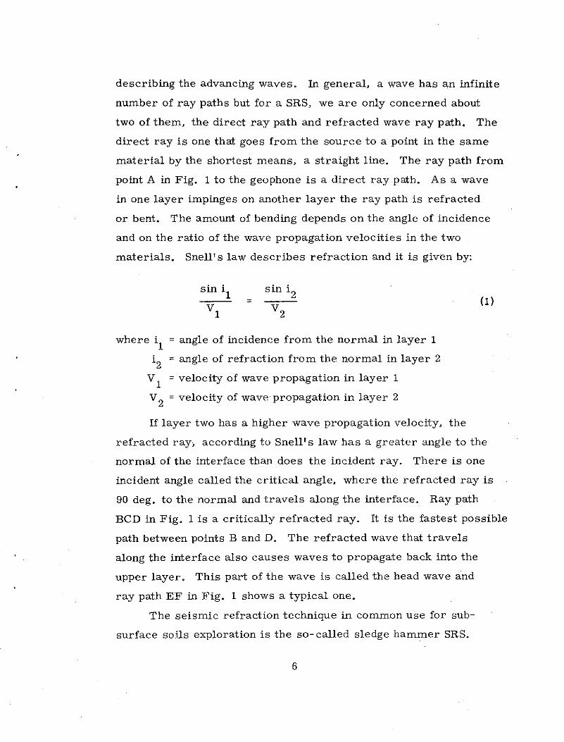
at the edge of the depression nearest the end of the survey and at the end of the survey are obtained by use of Fig. 10.

7) The hump begins approximately where the data begins deviating from the reference depth line. The point where the maximum deviation occurs is the highest part of the hump. The total travel time at this point is used in Fig. 11 to calculate the height of the hump. The end of the hump exists approximately where the data starts deviating from the reverse profile reference depth travel time line.

The procedure just outlined is relatively cumbersome and the

results are not all that accurate (the causes for errors will be dis­

cussed later). As a result, a simplified procedure is recommended.

This procedure is identical with the one just outlined except that

Steps 6) and 7) be qualitatively applied. The first steps provide a

reference depth line, velocity data for the two materials and refer­

ence depth travel time curves. The velocities are quite helpful in

determining soil moduli (see Ref. 9) and the reference depth line

travel time curves provide an excellent frame of reference for

evaluating the travel time data. Depressions and humps then can

be quickly noted. Detailed dimensions of these can then be obtained

by more positive techniques such as sounding and boring.

Description of Field Test Sites - Four test sites were used. The

first site was bcated on the University of Kentucky campus near the

corners of University and Cooper Drives. Bedrock was fairly

level and uniform. Two to fourteen feet of residual clayey silt

covered the rock.

The second site was located west of the city of Lexington on

the University of Kentucky Poultry Research Farm. Advanced

stages of solutioning existed at this site. Excavations for buildings

revealed the existence of pillars of resistant limestone referred to

20

«> I Actual TT Procedure ~T _____ )(~=:, Curve 1. Cale. L~ixi~-Xdl '" --------- 2.Calc.M=v~~1+L2 ~t -- 1 ~1 LRef. Depth 3 C I N = L Line · a c. .... . . (tv. ~

Distance from Geophone ~ _H2-M)*

Vet. = V1 4. From part b get 8. ....--4--+-Geophone H ' B

x1 ---t-B-1 from N and ~1 -""l'P"',Wlw,'"""""~

Vel.=V2

4.--~-r-~.--..---.--,--T""W'7...,.,....---,,...........,...---T-.-~

(b)

2

1

0 .5 1 2 5

5

10

10 N

20 x~ B

50

FIG. 9 PROCEDURE FOR EST. DEPTH OF CHANNEL

21

"O c: w >, Q)

> ... j

(/) -<l .10

I~: Q)

E .01

I- ----- -----.05

~ · Xe= Dist. From Geophone To Center Line.Of Chonne -~ cE ~Te V2 = (1- ~)2 + (.A. )2 + (~ )2+(.A.) .... Xs Xs Xs Xs Xs ~ . 0 0 I O .2 .4 . 6 .8 I.

Xc/Xs

. Q) c: c: 0 .c u

.IO....----....--.-----....--....--.....--.....--....---

-0 Q) c,, 'O w

I.

- >N <l O

I- x ~ <I c:

Q)

E 1-'0 Q) N

0

E .... 0 z

0.1

0.01 0

~ TX~2 =J(fxc)2+( ~c )2+J1 +(A/Xcl2'_&c-1

2.----------------1 -----1.------~

------- 0. 5 -------.J

.2 A .6

0.2 ------..J A/Xe

0.1

.8 I. 1.2 8/Xc

1.4 1.6 1.8 2.0

Fig. 10 Corrections For Ref. Depth Travel

22

Time Curve Due To Channel.

Q)

E Reference Depth TT Lin~e>--- - -- - -Actual TT -G>l__...-~-----~~:::::::::=--..--!:!~=- Curve

~ I/________..!.... f L t I-

Distance from Geophone

.---+-+-Geo phone

. X1~

t H

A H

FIG. 11

A

1.0..---,........,---.---........ --.----........... ---,

.8

.6

.4

.2 ~ V

1.5 2.5 4.0 5.0 10.0 1

0 2 4 6 8 R=tV2-X1

H PROCEDURE FOR DETERMINING HUMP

23

10 12

HEIGHT OF

as solution pinnacles. A sinkhole was also present on this site.

Depth to rock varied from zero to 20 ft.

The third site was north of Lexington where the new U.S.

Post Office is being constructed. Explorations at this site revealed

both early and intermediate stages of solutioning depending on

location on the site. Depth to rock varied from Oto 15 ft.

Finally, the la.st site was located on alluvial silts and sands

adjacent to U. S. Army Corps of Engineers Lock and Dam No. 9 on

the Kentucky River near Valley View, Kentucky. Because bedrock

was so deep, profiling could not be done.

Typical Field Travel Time Curves - Travel time curves at the

Campus site and at the Lock 9 site gave relatively smooth travel

time curves. The velocity of the second layer at the Campus site

was due to rather substantial limestone bedrock. At one location,

the data indicated a hump in the rock surface as shown in Fig. 12.

Subsequent proof drilling revealed a layer of resistant rock at

approximately the predicted elevation but the drill could penetrate

the layer and bedrock was actually established at a depth of 13. 5

ft. The resistant rock layer is frequently encountered and is re­

ferred to as a floater. In this case, the floater was masking the

location of a channel.

At the Lock 9 site, bedrock was not encountered with the

drilling equipment available. It was estimated to be around 75 ft

below the surface. Seismic surveys were performed at interfaces

of different soil layers for the purpose of gaining velocity and

modulus information. This is reported in Part II of this report. (9)

For the other two sites, travel time curves were quite

undulating as shown in Fig. 13 for example. Undulations in the

rock surface was the main cause of the nonuniformity of travel

times but other causes such as velocity variations in the soil and

24

15 -"' E -Q)

E I- 10

Q)

> 0 .... I-

5

O L-~~..i...~~-'-~~~L....~~..i...~~-'

0 10 20 30 40 50

Distance Along Survey (ft)

A

45

-- 10 Predicted From -- , /.,

-c. Q)

a

SRS Ji Drilling Data~

20

Fig. 12 Travel Time Curve And Data Reduction At Campus Site.

25

-c., Cl)

(II

- E -Cl)

(a)

16• , J I I _ I I

12

---E 8 I-

Cl)

> c ... I-

~ .... --.c .... 0. Cl)

Cl

~ ..... Field Data 4

- -- Boring Profile -- Predicted Profile

0 0 10 20 .30

A Horizontal Distance

BH504 0

' Reference 5

10

15

40 50

( ft ) B

BH 503

Predicted Rock Surface Profile Data Points Are From Borings

( b)

Fig. 13 (a) Field And Computer Generated Travel Time Curves, (b) Predicted And Observed Rock Surface Profiles.

26

data interpretation were also ca.uses. Forward and reverse profile

data generally were consistent. In a few cases they were not, and

determining the reason was difficult if not impossible.

Methods of Checking Rock Surface Profiles - At two sites excava­

tions near the seismic refraction survey locations enabled at least

a general check on the predicted results. At the Campus site a

relatively flat rock surface profile was predicted and excavations

revealed the same. More accurate definition along each profile

was achieved using machine auger borings with a CME model 55

drill rig. Spacings were generally 10 ft. on center but occasionally

these were reduced at specialized locations. A second and quicker

method utilizing the Dutch Cone Penetrometer was also used.

Details of this method are given in a thesis by Cleveland (10) and

also reported by Drnevich (11). In addition to locating the rock

surface, this sounding method gave information on the variability

of the soil with depth. Correlation with strength characteristics

were also made.

Comparison of Predicted and Measured Rock Surface Profiles -

The procedure outlined earlier was used on a number of the surveys.

The results of a survey at the Campus site are given in Fig. 12

which has already been discussed. Most of the results for the more

complicated profiles were in qualitative agreement (i. e. humps

existed where travel time curves were below the reference depth

travel time curve and depressions existed where the actual travel

time curves were greater than the reference depth travel time

curves). The method developed was still somewhat subjective and

tended to break down where depressions or sinks were very shallow

and wide. A typical predicted rock surface profile for one of the

more complicated travel time curves is given in the lower portion

of Fig. 13. The depths to the rock surface from proof drilling are

27

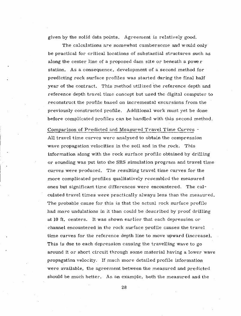
given by the solid data points. Agreement is relatively good.

The calculations are somewhat cumbersome and would only

be practical for critical locations of substantial structures such as

along the center line of a proposed dam site or beneath a pO\re r

station. As a consequence, development of a second method for

predicting rock surface profiles was started during the final half

year of the contract. This method utilized the reference depth and

reference depth travel time concept but used the digital computer to

reconstruct the profile based on incremental excursions from the

previously constructed profile. Additional work must yet be done

before complicated profiles can be handled with this second method.

Comparison of Predicted and Measured Travel Time Curves -

All travel time curves were analyzed to obtain the compression

wave propagation velocities in the soil and in the rock. This

information along with the rock surface profile obtained by drilling

or sounding was put into the SRS simulation program and travel time

curves were produced. The resulting travel time curves for the

more complicated profiles qualitatively resembled the measured

ones but significant time differences were encountered. The cal­

culated travel times were practically always less than the measured.

The probable cause for this is that the actual rock surface profile

had more undulations in it than could be described by proof drilling

at 10 ft. centers. It was shown earlier that each depression or

channel encountered in the rock surface profile causes the travel

time curves for the reference depth line to move upward (increase).

This is due to each depression causing the travelling wave to go

around it or short circuit through some material having a lower wave

propagation velocity. If much more detailed profile information

were available, the agreement between the measured and predicted

should be much better. As an example, both the measured and the

28

predicted rock surface profiles in the bwer portion of Fig. 13 were

put into the simulation program. The calculated travel times are ·

given in the upper portion of Fig. 13 by the dashed and the solid

curves, respectively. Note that the agreement is much better using

the predicted profile because it gives the profile (especially the

depress ion) in greater detail.

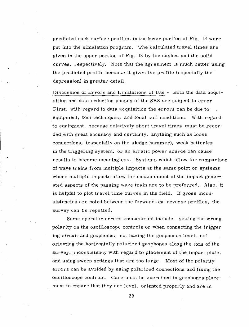
Discussion of Errors and Limitations of Use - Both the data acqui­

sition and data reduction phases of the SRS are subJect to error.

First, with regard to data acquisition the errors can be due to

equipment, test techniques, and local soil conditions. With regard

to equipment, because relatively short travel times must be recor­

ded with great accuracy and certainty, anything such as loose

connections, (especially on the sledge hammer), weak batteries

in the triggering system, or an erratic power source can cause

results to become meaningless. Systems which allow for comparison

of wave trains from multiple impacts at the same point or systems

where multiple impacts allow for enhancement of the impact gener­

ated aspects of the passing wave train are to be preferred. Also, it

is helpful to plot travel time curves in the field. If gross incon­

sistencies are noted between the forward and reverse profiles, the

survey can be repeated.

Some operator errors encountered include: setting the wrong

polarity on the oscilloscope controls or when connecting the trigger­

ing circuit and geophones, not having the geophones level, not

orienting the horizontally polarized geophones along the axis of the

survey, inconsistency with regard to placement of the impact plate,

and using sweep settings that are too large. Most of the polarity

errors can be avoided by using polarized connections and fixing the

oscilloscope controls. Care must be exercised in geophones place­

ment to ensure that they are level, oriented properly and are in

29

firm contact with the soil or rock. Sweep rates should be set such

that the horizontal portion of the trace covers at least half the width

of the screen. With regard to the pl~ement of the impact plate, a

cloth measuring tape stretched along the survey axis and held in

place by taping pins is quite helpful. Also, the sod and any organic

material that might prevent a firm impact with the soil is removed

at each impact point.

For the SRS to be accurate, soil conditions must be relatively

uniform over the length of the survey. When making the borings

at the ends of the survey for down hole shooting it is wise to log

the soils encountered. If the bgs show vastly different soil conditions,

the SRS will be subJect to considerable error.

Data reduction errors begin with determining the travel time

for the first arrivals. If an oscilloscope is used to measure travel

times, the travel time is proportional to the horizontal portion of

the trace. It is tempting to take the point where the trace begins

deviating from the horizontal. However, errors on the order of

one millisecond can be caused by simply changing the vertical

amplifier gain setting or by ambient noise. A more accurate prac­

tice is to choose the point corresponding to the intersection of the

horizontal portion and a tangent to the slope of the first wave.

The procedure for determining the reference depth line is

no problem. Accurate determinations of the velocities is not always

foolproof. The velocity in the soil is the average compression wave

propagation velocity in the vertical direction. If several soil layers

are encountered, the velocity measured in down hole shooting will

be weighted average of the velocities in each layer. If the layer

thicknesses are relatively consistent over the survey length, these

should be no problem. However, if the geophones themselves are

located in a narrow depression or very close to a solution pinnacle,

30

then the value of velocity for the soil will be high. Use of a higher

than actual velocity in the profile determination procedure will

exaggerate the deviations from the reference depth line.

All depressions of the rock surface beneath the reference

depth line cause an increase in the ray path length of the first

arrival. As a consequence, the value of velocity given by Eq. 4

will be lower than actual. Correction of the values given by Eq. 4

based -on a ratio of areas beneath the travel time curves and the

line connecting the end points of the travel time curve appears to

give much better results.

Another source of difficulty in determining the values of

velocity is the presence of water. First of all, if the water table

is above the rock surface both the velocity values in the soil and

the rock will be distorted. In saturated porous media, a compression

wave can travel through the fluid at a velocity which is usually be­

tween 4500 and 5000 ft/ sec. If the wave propagation velocity in the

rock is in this same range, it will be impossible to distinguish

between the soil and the rock. If the wave propagation velocity is

much higher then the presence of water will tend to mask the undula­

tions in the rock surface and the procedure suggested earlier will

underestimate the deviations from the reference depth line. Addi­

tional work to study the effects of the water table is certainly

needed.

The data reduction procedure suggested earlier assumes tw::i

dimensional conditions whereas in the field wave ray paths are not

restricted to two dimensions. Consequently, the calculated pro­

files will be somewhat in error. For example, if the survey were

run along the axis of a very narrow solution channel, it would not

be detected. Likewise, if a solution pinnacle were not on the survey

line but were close to it, it would be picked up. An extreme

31

j

example of this case would involve running a survey adjacent and

parallel to a concrete pavement. The survey results would show a

"rock surface" at a depth equal to the distance between the survey

line and the pavement.

Finally, there exists some limits of depth and size that must

be discussed. Reasonably accurate data were obtained with the

equipment and techniques described earlier for depths of the rock

surface less than 20 ft. At one site the depth to rock was greater than

50 ft and no profile data could be obtained. Based on the field

tests in this program, it is estimated that a practical limit for rock

surface profiling where the sledge hammer SRS is used is on the

order of 25 to 30 ft. This may also be a limit when explosive sources

are used because localized velocity variations in the soil would pro­

vide more variations in travel times than undulations in the rock

surface profile. Thus accuracy of profile determination diminishes

with depth to rock surface.

Besides the limitations described above, there are limits on

the size of an anomaly that can be detected. Consider a very deep

channel in the rock surface that has a width B. The maximum in­

crease in the travel time that this channel can cause is B/V 1

where

V 1

is the wave propagation velocity in the soil. In terms of typical

values, deviations in travel times less than a half a millisecond are

too small to consider and values of V 1

are on the order of 1500

ft/ sec. This means that for ideal conditions, channel widths less

than 0. 75 ft cannot be detected. Under typical situations this

minimum is increased to about 2 ft.

The procedure for determining the depth of channel is based

on the first arrival travelling around the channel. For a channel of

given depth there is a minimum width below which the first arrival

"short circuits" through the channel. Normalized minimum widths

32

•

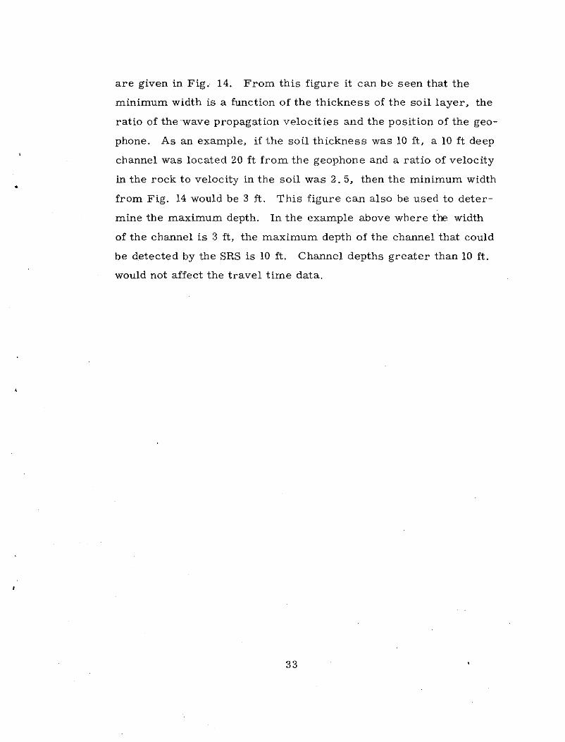
are given in Fig. 14. From this figure it can be seen that the

minimum width is a function of the thickness of the soil layer, the

ratio of the ·wave propagation velocities and the position of the geo­

phone. As an example, if the soil thickness was 10 ft, a 10 ft deep

channel was located 20 ft from the geophone and a ratio of velocity

in the rock to velocity in the soil was 2. 5, then the minimum width

from Fig. 14 would be 3 ft. This figure can also be used to deter­

mine the maximum depth. In the example above where the width

of the channel is 3 ft, the maximum depth of the channel that could

be detected by the SRS is 10 ft. Channel depths greater than 10 ft.

would not affect the travel time data.

33

'-" ,!>-

.e. H

4 /Geophone n -I Bt- H V1

.. . I A v2 ·x

I ""

3

I ~I = 0 I I ~ I = 2 I 2

0~10. O I I I 1

I A/H

2 0 I A/H

I ~I =41

2 0 I A/H

2

Fig. 14 Minimum Normalized Channel Widths For First Arrival Roy Poth Around Channel.

CHAPTER IV

CONCLUSIONS

The down hole shooting seismic refraction survey method has

definite advantages when rock surface profiling is desired. This

includes: calibrations at the ends of the survey, direct measure­

ment of the soil velocity in the vertical direction and having the

refracted wave being the first arrival over practically the entire

survey length.

The seismic refraction equipment used for this research work

was satisfactory although improvements in the equipment are both

possible and desirable to reduce the possibility of operator error

and to increase accuracy.

The computer simulation method is certainly a helpful tool

for studying the characteristics of seismic refraction in compli­

cated situations. It is also helpful in checking the accuracy of cal­

culated rock surface profiles.

The data reduction procedure developed herein can handle

relatively complex profiles. The concept of reference depth line

and its associated travel time curves are most useful in assessing

the nature of the rock surface. The procedure for estimating the

deviations from the reference depth line is somewhat cumbersome

and requires some subJectivity. It appears that a completely gen­

eral method is feasible and future efforts should be directed toward

developing it. Most likely it would have to be a computerized

method to make it practical.

The accuracy of the seismic refraction survey for rock sur­

face profiling is a function of the nature of the soil and rock

35

conditions as well as a function of the methods used to obtain and

reduce the data. In general, the deeper the rock surface the less

the accuracy. For the sledge hammer survey, a depth of 25 to

30 ft appears to be the maximum for rock surface profiling. The

existence of a water table and three dimensional effects are also

causes for reduced accuracy. There is a minimum width of channel

that can be detected which appears to be about two feet. Also, for

a given channel width, there is a maximum channel depth that

can be detected with seismic methods. Approximate values for

these are given herein.

Finally, the seismic refraction survey is definitely a useful

tool for rock surface profiling. It can be used efficiently to inter­

polate between boreholes and very quickly establish locations where

additional investigation with conventional boring techniques should

be undertaken.

36

REFERENCES

1. Hays, J. B., 11 Deep Solution Channel, Kentucky Dam, Kentucky, Proceedings, ASCE, Vol. 69 No. 9, Nov., 1943, pp. 1400-16.

2. Bishop, Charles S., "Some Engineering Aspects of Kentucky Geology," Technical Report UKY 41-71-CE9, Soil Mechanics Series No. 6, College of Engineering, University of Kentucky, 1971, 29 p.

· 3. Anderson, L. R., and Girdler, H. F., "Detailed Rock Profiling by Seismic Refraction," Special Report, College of Engineering, University of Kentucky, Lexington, January 1970, 60 p.

4. Griffiths, D. H., and King, R. F., Applied Geophysics for Engineering and Geologists, Pergamon Press, New York, 1965.

5. Richart, F. E., Jr., Hall, J. R., Jr., and Woods, R. D., Vibrations of Soils and Foundations, Prentice-Hall, Inc. Englewood Cliffs, New Jersey, 1970, 414 p.

6. Wu, T. H., Soil Dynamics, Allyn and Bacon, Boston, 1971, 272 p.

7. Taanila, P., "A Profile Calculation Method in Seismic Refrac­tion Surveys Based on the Use of Effective Vertical Velocity, Geoexploration, Vol. 1, 1963, pp. 36-49.

8. Smith, S. R., "Location and Depths of Subsurface Undulations by Seismic Methods, 11 A thesis submitted in partial ful­fillment of the requirement for the degree of Master of Science at the University of Kentucky, 1971, 82 p.

9. Drnevich, V. P., "Location of Solution Channels and Sinkholes at Dam Sites and Backwater Areas by Seismic Methods,

10.

11.

Part II - Correlation of Seismic Data with Engineering Properties, 11 Research Report No. 55, Project A-026-KY, University of Kentucky Water Resources Institute, 0. W.R. R., August, 1972, 23 p.

Cleveland, E. P., "Use of the Dutch Cone Penetration Test for Soil Exploration in Kentucky," A thesis submitted in partial fulfillment of the requirements for the degree of Master of Science in Civil Engineering at fue University of Kentucky, 1971, 82 p.

Drnevich, V. P., "Exploration Methods, 11 Proceedings of the ASCE Ohio Valley Soils Seminar, Louisville, Ky., October, 1971, 43 p.

37

s n

s forward s

reverse T

TA

TB

AT

ATAB

ATB

x c

APPENDIX-I. -NOTATION

= channel depth or hump height

= channel or hump width

= thickness of soil layer

= thickness of soil layer at point A

= thickness of soil layer at point B

= ray path incident angle

= ray path refracted angle

= change in horizontal distance from soil surface to rock surface

= slope of line on travel time plot connecting the travel time at the beginning and end of the survey

=

=

=

=

=

=

S for the forward profile n

S for the reverse profile n

travel time

reference depth travel time line intercept at A

reference depth travel time line intercept at B

change in travel time for reference depth travel time line at the end of a channel

= change in travel time between AB for reference depth travel time line

= change in travel time at point B (end of the survey) due to a channel along the survey

= distance from geophone along survey

= distance from geophone to edge of a hump or a depression

= distance from geophone to the center line of a hump or a depression

= distance from the geophone to the point that causes the refracted wave to be the first arrival

38

x s = survey length

= angle between the reference depth line and the horizontal

39

APPENDIX II

SEISMIC REFRACTION SURVEY SIMULATION PROGRAM

$JOB

C DRNEVICH SEISMIC REFRACTION SIMULATOR FOR DOWN HOLE SHOOTING

C NSETS=NO OF PROFILE DATA SETS THAT ARE TO BE SOLVED IN ONE RUN

C V(l)=WAVE PROPAGATION VEL IN TOP LAYER

C V(2)=WAVE PROPAGATION VEL IN BOTTOM LAYER

C NSEG=NO. OF LINE SEGMENTS l'EEDED TO SIMULATh SOIL ROCK INI'ERFACE (MAX=40)

C NDS=NO OF DIVISIONS THAT SURVEY IS TO BE DIVIDED (MAX=400)

C XL(J),XL(J+L) = X-COORD OF J-TH SEGMENT ENDPOINTS

C YL(J),YL(J+L) = Y-COORD OF J-TH SEGMENT ENDPOINTS

C ND(J) = NO OF DIVISIONS THAT J-1H SE(l'illlT ISIDBE DIVIDED (MAX=40)

c DIMENSION XL ( 41), YL( 4l);v (2),ND(41), X(41, 41), Y (41, 41.), SL ( 41) , T ( 41,

141),XT(401),TT(401),DL(41),DXL(41),DYL(41),DND(41)

READ(5, 90)NSETS

90 FORMAT (11)

DO 500 NNN=l,NSETS

READ(S,100)V(L),V(2),NSEG,NDS

100 FORMAT(2Fl0.0,2I5)

NPTS=NSEG+l

READ(5,110)(XL(J),YL(J),J=l,NPTS)

110 FORMAT(l6F5.0)

READ(5,112)(ND(J),J=l,NSEG)

112 FORMAT(l615)

NTIME=O

WRITE(6,113)

113 FORMAT(lHl, 'FORWARD PROFILE CALCULATION')

C CALC OF COORD POINTS AND SEGMENT SLOPES

40

115 DO 150 J=L,NSEG

XC=(XL(J+l)-XL(J))/ND(J)

YC=(YL(J+l)-YL(J»/ND(J)

IF(XC.NE.O) GO TO 120

SL (J) =YC/ ABS (YC) *10**6

DL(J)=ABS(YC)

GO TO 121

120 SL(J)=YC/XC

DL(J)=ABS(XC)*SQRT(l+SL(J)**2)

121 X(l,J)=XL(J)

Y (1, J) =YL(J)

N=ND(J)+l

DO 150 1=2,N

X(I,J)=X(I-1,J)+xc

150 Y(I,J)=Y(I-1,J)+YC

WRITE (6,160) V(l),V(2),NSEG

160 FORMAT (1H0,4X, 'V(l)=',FIDO, 'V(2) = 'flO. 0, 'NO.OF SEGMENTS=', 15)

WRITE(6,170)

170 FORMAT(lHO, 4X,' POINT X-COORD Y-COORD')

WRITE(6,180)(J,XL(J),Yi.(J),J=l,NPTS)

180 FORMAT(lH ;4X,13,4X,F5.l,4X,F5.l)

C CALC OF TRAVEL TIMES ALONG INTERFACE

T(l,l)=O.

200 DO 250 J=l,NSEG

IF(J.NE.l) T(l,J)=T(ND(J-l)+l,J-1)

DT=DL(J) /V(2)

N=ND(J)+l

DO 250 1=2,N

T(l,J)=T(l-1,J)+DT

IF(J.EQ.l) GO TO 250

210 SMAX=SL (J)

SMIN=SL(J)

Jl=J-1

DO 242 JC=l,Jl

41

JB=Jl+l-JC

NN=ND(JB)

DO 240 IC=l,NN

IB=NN+l-IC

XC=X(I,J)-X(IB,JB)

YC=Y (I ,J)-Y (IB ,JB)

lf(XC.NE.0) GO TO 220

TSL=-YC/ AB~ (YC) *10''*6

DL2=ABS(YC)

GO 10 230

220 TSL=YC/XC

DL2=Al3S (XC) *SQRT(l .+1 SL''*2)

230 IF(XL(J+l)-XL(J).LT.O.) GO TO 232

231 lf(TSL.GE.SMAX) GO TO 235

IF(TSL.GT.SMIN) GO Tll 240

GO TO 233

232 IF(SL(J).GT.0.) GO TO 234

IF(TSL.LT.O.) GO TO 231

SNIN = 10''*6

IF(TSL. LE. SNII':) GO TO 233

GO TO 240

234 IF(ISL.GT.O.) GO TO 211

sw,x =-10''*6

IF(TSL.GE.SMAX) GO TO 235

GO TO 240

233 SMIN =TSL

VEL=V(2)

GO TO 236

235 SMAX=TSL

VEL=V ( 1)

236 T2=DL2/V£L +T(IB,JB)

IF(T(l,J).LT.T2) GO TO 240

237 T(l,J)=T2

240 CONTBUL

42

242 CONTINUE

250 CONTINUE

WRITE(6,260)

260 FORMAT(1H0,4X,"X(I,J) Y(I,J) T(I,J)')

DO 280 J=l,NSEG

N=ND(J)+l

DO 280 I=l,N

IF(l.EQ.N.AND.J.NE.NSEG) GO TO 280

WRITE(6,270)X(I,J),Y(I,J),T(I,J)

270 FORMAT(lH,4X,F6.2,F8.2,2X,F7.5)

280 CONTINUE

C CALCULATION OF TIME FROM INTERFACE TO SURFACE

XT (1)=0.

DX=XL(NPTS)/NDS

NSPTS=NDS+l

TT(l)=YL(l)/V(l)

DO 282 L=2,NSPTS

XT(L)=XT(-l)+DX

282 TT (L) =SQRT (XT (L) ''*2+YL (1) **2) /V ( 1)

DO 400 J=l,NSEG

N=ND(J)

00400 l=l,N

IF(Y(I,J).EQ.O.) GO T0.321

Sl=X(I,J)/Y(I,J)

S3=(X(I,J)-XL(NPTS))/Y(I,J)

290 DO 320 K=l,NPTS

XC=X(I,J)-XL(K)

YC=Y(I,J)-YL(K)

IF(YC.EQ.O.) GO TO 320

IF(XC.LT.O.) GO TO 300

S2=XC/YC

IF(S2.LT,Sl.AND.S2.GE.O.) Sl=S2

GO TO 320

300 S4=XC/YC

IF(S4.GT.S3.AND.S4.LE.O.) S3=S4

43

320 CONTINUE

321 CON'l'INUt

YC=Y(I,J)

DO 360 L=l,NSPTS

XC=X(I,J)-XT(L)

IF(YC.EQ.O.) GO TO 340

SS=XC/YC

IF(SS.GT.Sl.OR.SS.LT.S3) GO TO 360

340 TL=SQRT(XC*XC+YC*YC)

TG=T(I,J)+TL/V(l)

IF(TG.LT.TT(L)) TT(L)=TG

360 CONTINUE

361 CONTINUE

400 CONTINUE

C WRITE RESULTS

WRITE(6,420)

420 FORMAT(llll,4X,'POINT X-COORD TRAVEL TIME'/)

WRITE(6,430) (L,XT(L) ,TT(L) ,L=l,NSPTS)

430 FORMAT(lH ,6X,I3,F8.l, Fll.5)

IF(NTIME.GE.1) GO TO 500

NTIME=NTIME+ 1

C REVERSE PROFILE CALCULATION

WRITE(6,440)

440 FORMAT(llll, 'CALCULATIONS FOR REVERSE PROFILE')

DO 460 J=J.,NPTS

DXL(J)=XL(NPTS)-XL(NPTS+l-J)

DYL(J)=YL(NPTS+l-J)

IF(J.EQ.NPTS) GO TO 460

DND(J)=ND(NPTS-J)

460 CONTINUE

DO 480 J=l,NPTS

XL(J)=DXL(J)

YL(J)=DYL(J)

IF(J.J::Q.NI'TS) GO TO 480

ND(J)=DND(J)

44

480 CONTINUE

GO TO ll5

500 CONTINUE

STOP

END

45