Location Decisions of Domestic and Foreign-Affiliated Financial Advisors: Australian Evidence

Robert W. Faff, Tribeni Lodh, Jerry T. Parwada*

Keywords: Financial advisors, Financial planning, Location choice

* Please address all correspondence to Jerry Parwada: Australian School of Business, University of New South Wales, UNSW Sydney, NSW 2053, Australia; Tel: +61 2 9385 7836, Email: j.parwada@unsw.edu.au. Faff is in the Department of Accounting and Finance at Monash University. Lodh is at Lehman Brothers Australia. The authors thank the Melbourne Centre for Financial Studies for providing funding and the Australian Securities and Investments Commission for data.

2

Location Decisions of Domestic and Foreign-Affiliated Financial Advisors: Australian Evidence

Abstract

This paper analyses the determinants of the start-up location choices for 54,064 Australian personal

financial advisors, and examines these choices with respect to their foreign and institutional affiliations.

The evidence presented suggests that advisors consider general socio-economic and financial

demographics when first choosing the location to commence their careers. Advisors tend to locate in areas

with high population, low unemployment, smaller households and more elderly persons. Competition does

not deter planners from choosing a particular location. Furthermore, foreign originated start-ups ignore

financial characteristics, and prefer to locate in regions in which general demographics indicate a large

market size. Bank affiliated start-ups locate in more favorable locations than independent advisors,

reflecting cost and informational advantages. Independent advisors demonstrate ‘learning’ by replicating

the location choices of institutionally linked advisors in the short term.

1. Introduction

The importance of the geographical location of economic activities has been investigated and

supported by various studies starting with Carlton (1983), which attempts to model the link between

location choice and economic variables specific to geographical regions. The literature also provides clear

empirical and theoretical evidence that several geographical factors influence foreign firms’ location

choices. For example, Woodward (1992) applied a similar model to explain the location determinants of

Japanese manufacturing start-ups in the US and found that Japanese investors prefer to locate in strong

markets with low unionization rates.

In relation to the financial services industry, the primary focus for location studies has been on the

banking industry (see Claessens Demirgüç-Kunt and Huizinga (2001) and Claessens and van Horen

(2007) for recent examples). Interest is growing on the location behavior of entities in the investment

3

management industry following compelling evidence of the performance relevance of investors’ proximity

to each other (Hong, Kubik and Stein (2005) and Ivković and Weisbenner (2005)) and target securities

(Coval and Moskowitz (1999, 2001)). Ruckman (2004) investigated how the level of fund- and firm-level

characteristics of US mutual funds affect the channel used to enter the Canadian market. Parwada (2008)

found that fund company start-ups tend to be based close to the origins of their founders, and in regions

with more investment management firms, banking establishments, and large institutional money

managers. Furthermore, a variety of social and economic attributes provide significant explanatory power

to the location choice model applied.

In this paper we contribute to the literature by examining the location behavior of financial advisors

and their role in the distribution of products in the investment management industry. We trace all

Australian Financial Services (AFS) representatives issued with licenses to provide personal financial

advice and examine the determinants of where they commence their careers. We refer to individual

representatives as financial planners or advisors and their affiliated organizations as financial planning

groups. To examine the link between the locations of financial advisors and the broad characteristics of

geographic locations, we use well-established location choice models. We hypothesize that three broad

classes of variables have significant explanatory power in relation to location choice; financial

demographics, general demographics, and competition demographics. We then extend the analysis by

relating it closely to the ownership structures of financial planning groups. Specifically, we use a hand-

collected database of parent company and institutional alliance information, including foreign parentage,

to examine the location choices of those advisors. The differences among advisory structures may imply

comparative advantages and could signal informational asymmetries (Ihlanfeldt and Raper (1990)).

The Australian setting presents an interesting laboratory in which to examine the strategic location

decisions of financial advisory service providers. Ranked fourth in the world by funds under management,

the industry is dominated by the distribution channel, fuelled largely by a rapidly expanding financial

planning industry that gives fund managers access to retail clients. Growth in the industry is also attributed

4

to the system of compulsory superannuation (or pension) contributions effective since 1992, strong equity

markets, and innovations in product design. The financial planning industry thus plays a crucial role in the

distribution of products.

The paper is organized as follows. Section 2 describes the hypothesis and the theoretical motivations

of the determinants considered. The compilation of the dataset is summarized in Section 4. Section 5

presents the methods adopted. Section 6 includes results of the empirical analysis. Section 7 concludes.

2. Developing the Hypotheses

In this section, we form two key hypotheses for the analysis. The first concerns the determinants

of the location choice of financial advisors. The second is founded on the idea that ownership structures

such as foreign and institutional affiliation affect the level of information available to advisors, leading to

differences in location choice criteria.

2.1. Determinants of Start-up Location Choice

Abstracting from the previous location choice literature we hypothesize that financial advisors

consider socioeconomic location characteristics when choosing the location of a start up.1 We divide the

proposed determinants into three broad categories; general demographics, financial demographics, and

competition demographics. The general demographics are included to account for advisor preference

towards areas with favorable social characteristics. Such preference may include high population, area,

and household size, all of which can be explained by the source funds hypothesis. Furthermore, a positive

test of the hypothesis provides insight into the effects of urbanization on location choice. Financial

demographics focus on monetary flows and financial characteristics. The proposed determinants income,

rent and loan repayments directly test the source funds hypothesis, while unemployment and the

proportion of fully owned dwellings are used as proxies to represent the financial stability of a particular

geographic area. Finally, competition demographics present variables describing the congregation of

related industries in particular physical localities. Specifically, these include the number of banking

1 See (Bartik (1985), Porter (1990), Ihlanfeldt and Raper (1990), Almeida and Kogut (1999), Shaver and Flyer (2000), Chung and Kalnins (2004), Kolko (2007), and Brandao and Mota (2006)).

5

organizations, credit unions and building societies in an area. With reference to Kolko (2007), which

found service industries to exhibit high levels of agglomeration, we hypothesize that the existence of

advisors and related industries in an area encourages the location decision of start ups.

2.2. Ownership Structures and Location Choice

We hypothesize that information asymmetries between foreign affiliated and domestic advisory start-

ups are reflected by their corresponding location choice behavior. Domestic advisors have the advantage

of prior knowledge and experience in the area. Furthermore, there is an increased likelihood that domestic

start-ups have relationships with existing providers of financial products. We hypothesize that foreign

originated start-ups suffer an initial disadvantage in this respect. The motivation is provided largely by

earlier research that suggests foreign investors are often assumed to be at a disadvantage on location

choice relative to locals. For example, Claessens, Demirgüç-Kunt and Huizinga (1998) note that the

technical advantages which foreign banks may have developed are not significant enough to overcome the

informational disadvantages they face relative to domestic banks. In the context of this study, this

disadvantage may be demonstrated via location choices that reflect a lack of specific market knowledge.

This effect is likely to be more profound during the start-up period, which is the focus of our study.

However, despite a possible informational disadvantage, foreign affiliated start-ups may be provided a

greater level of financial backing than domestic counterparts, particularly over those practices which are

independent of any institutional affiliation.

Institutional ownership of an advisory practice is hypothesized to change the manner in which

advisors choose to locate. The reasons for this difference can be explained based on an examination of the

nature of independent and institutionally linked advisory practices. The location choice behavior between

the two types of advisors may differ for several reasons. Firstly, institutionally linked advisors will likely

place a considerable bias on their role in the distribution of financial products on behalf of their owners.

The specialty of the advisory and the type of product should affect the location demographics targeted. For

example, in the case of retirement products offered by a bank, advisors can take the strategy of locating in

6

areas with higher numbers of aged citizens. Secondly, independent advisory practices, which receive no

financial or promotional backing, are likely to have a lower propensity than institutionally linked advisors

to locate in areas with higher competition. This introduces the idea of collocation, and whether the two

advisory structures approach agglomeration of financial services in the same way. Finally, institutionally

linked advisors will account for existing business units of that organization in a particular area.

Furthermore, they may also consider the organization’s current brand power in an area.

3. Data, Institutional Background and Variable description

Financial planning firms themselves can be divided into the licensees whom the responsible parties

hold accountable to ASIC’s stringent regulations for financial advice, and the authorized representatives

which fall under a single license holder. In general, licensees represent larger companies and dealer groups

(networks of financial planners), and are ultimately responsible for the advice given by the representatives

they have placed.

Table 1 lists the top 20 financial planning dealer groups ranked by the number of advisors. As evident

from Table 1, the distribution of advisors is very heavily skewed towards the top 5 dealer groups.

Furthermore, large banks and fund managers, who gain synergies via product distribution channels,

dominate ownership of the dealer groups. Several of these parent companies make up the top 10 providers

of retail and wholesale investment products in Australia, which are listed in Table 2.

The analysis of location choice introduces several data collection challenges. The first major

challenge concerns the collection of community characteristics, which are difficult to obtain on

geographic divisions that allow for analysis of community differentials. For example, data for state and

metro level comparisons are readily available; however postcode level data can only be obtained via a

nationwide census. Furthermore, it may not be possible to match the periods in which data are collected.

Postcode analysis must be performed using statistics published from the nationwide census, which

unfortunately takes place every 5 years. This is problematic from a modeling perspective, especially if the

7

data are merged with advisor and other financial data obtainable on an annual or, often, quarterly basis.

The second major challenge concerns the collection of advisor location information. Since all published

records of financial planning agencies focus on their initial registration date, the study is limited to the

analysis of the entry decision of planners, and is not able to further examine their possible relocations for

any persistence in location choice behavior.

We use two main forms of data in this study. First, advisor level information detailing the location of

the financial advisors under analysis, and second, location data comprising location specific socio-

economic characteristics.

3.1. Advisor-Level Information

These data comprise location information for 54,064 Australian Financial Services (AFS)

representatives issued with licenses listed under the Australian Securities and Investments Commission’s

(ASIC) AFS Licensee Register as at October 23, 2006. Formally, AFS representatives are defined as those

authorized to provide financial services on behalf of the license holder. Despite the broad composition of

the financial services industry, the majority of license holders operate traditional financial planning

companies. More specifically, financial planning services include risk management, stock broking

operations, retirement planning, as well as tax, investment and superannuation advisory.

Aside from representatives, we obtain data for the 1,502 licensees under which individual planners

are registered. Locations are all represented on the 4-digit postcode level, which is a fine enough level to

meaningfully differentiate community characteristics.2 The use of the postcode also allows for analysis on

the 3-digit level, which represents a broader regional perspective. In cases where representative locations

are classed as missing in the database, we use the licensee locations as substitutes. This approach is

reasonable since these cases are largely restricted to small independent licensees. Furthermore, areas

which have been created to account for large mail volume receivers (e.g. Universities) are replaced with

the corresponding geographical postal area in which they are located. The same treatment is applied to

2 Postcodes in Australia are analogous to Zip Codes in the U.S.

8

post office boxes. The database has the advantage that registration data of all planners can be divided into

those commencing operations in each year from 2002 to 2006, providing the opportunity to witness the

change in location choice of start-ups over time.

Descriptive statistics for AFS representatives and licensees are given in Table 3. Panel A presents the

state level distribution of advisor locations, as well as the proportion of advisors in each state that are

located in the corresponding financial centers. Panel B lists the top ten postcodes from a total of 1,682,

ranked by the number of representatives and licensees respectively. Panel C provides a breakdown by year

of registration.

As evident from Panel A, the majority of financial advisors choose to locate in New South Wales,

Victoria, and Queensland, the three most heavily populated states in Australia. Furthermore, a large

proportion of those representatives choose to locate in the financial centers of those states with 16%, 12%,

and 10% in Sydney, Melbourne and Brisbane, respectively, while several other centers have higher levels.

Also as expected, the highest ranked postcodes in Panel B are generally the financial centers, with the top

ten 10 accounting for 17% of the total number of representatives. The importance of this is that the

congregation in regions of increased financial activity may bias the results of analysis. For this reason we

will introduce control variables, which are detailed in Section 5.

The geographic distribution of licensees is significantly different from that of representatives. Panel

A indicates significant clustering, with 1,233, or 83% located in Queensland. Surprisingly, only 1% of the

licensees in Queensland are located in the financial centre of Brisbane. However, upon investigation of the

top 10 postcodes in Panel B we can see that 1,195 licensees are located in the Gold Coast region of

Queensland, representing 97% of all licensees in the state. Interviews with practitioners suggest this

unbalanced distribution is explained by the influx of financial advisers chasing retirees who have recently

settled in the area in large numbers.

For those advisors that are not independent (i.e. dealerships which are not advisor owned), identities

and locations for the corresponding parent companies are hand collected via the use of fund manager

9

directories, Factiva and relevant news articles. Henceforth, we refer to these dealerships as ‘institutionally

linked’ advisors. Parent companies are classed into three main industry categories; banking, investment

management, and insurance. Furthermore, we divide the sample into domestic and foreign parents.

Banking organizations are categorized using the list of authorized deposit-taking institutions (ADI’s)

defined by the Australian Prudential Regulatory Authority (APRA). This classification includes Australian

owned and foreign banks, which incorporates both Australian branches of foreign banks and subsidiaries

of foreign banks. A summary of the advisor ownership is presented in Table 4, which shows a breakdown

of advisors by independence (i.e. advisor owned) in Panel A and parent companies by primary industry of

operation in Panel B.

Panel A of Table 4 reinforces the difference in characteristics between representatives and licensees,

with 54% of advisors being independent, compared with 85% for licensees. There are a total of 143

different parent companies with controlling interests in the non-independent advisors in Panel A. The

majority of parent companies are involved in the banking and investment management industries with a

total of 26 and 65 subsidiaries, respectively.

3.2. Location Characteristics Data

Location specific data are obtained from the 2006 Australian Census as provided by the Australian

Bureau of Statistics (ABS), which aims to accurately measure Australia’s population on the census night

in addition to socio-economic characteristics of the population and the dwellings in which they live.

Census data are collected at the postcode level. In total, the ABS publishes data for 2,524 different

postcodes. While merging the location data (which are provided for a single point in time) with the

advisor location data (provided annually), we assume that the characteristics collected via the census are

constant across the five years under consideration. Thus the resulting dataset includes 12,620 (2,524*5)

observations. Of the 2,524 postal areas in Australia, 607 are located in New South Wales, 655 in Victoria

and 432 in Queensland. These three states represent 67% of the postcode distribution. Descriptive

10

statistics for the postcode data are presented in Panel A of Table 5. Panel B provides a matrix of

correlations of all independent variables considered in the analysis.

In Panel A of Table 5, the census data are divided into three main classes. The first class includes the

financial demographic variables of INCOME, RENT, loan repayment (LREPAY), the proportion of

dwellings which are fully owned (OWNDW), and the unemployment rate (UNEMP). Together, the

financial demographics represent the level of source funds available and the financial stability of an area.

Income is defined as the median weekly individual income in each postcode. RENT is the median weekly

rent collected for dwellings in each postcode, while loan repayment represents the median monthly

housing loan expense, and is applicable to occupied private dwellings being purchased as well as

dwellings being purchased under a rent/buy scheme. The proportion of dwellings fully owned represents

the average tenure type in a given location, and is calculated after excluding those dwellings occupied

under any type of rental agreement. The unemployment rate (UNEMP), as provided by the ABS, is

calculated as the total number of persons unemployed expressed as a percentage of the labour force.

The second class of variables used are general demographic variables, and are included in the model

to account for systematic differences in social characteristics of a location. These include the area’s

population (POP), the AREA (in square kilometers), the median AGE of all persons, and the average

household size (HSIZE), which is defined as the number of persons usually resident in occupied private

dwellings. The education level (EDUC) has also been estimated as the proportion of persons to have

completed year 12 or equivalent as their highest year of education. Finally, a dummy variable (METRO)

is included classing postcodes as metro/non-metro, by adopting classifications published by Australia

Post.

The third class of location specific information is obtained by merging the census data with point of

presence (PoP) data obtained from APRA. The data provide the number of existing financial services

organizations in Australia on the postcode level. Organizations of particular interest to this study are the

number of building societies (NBDS), credit unions (NCRU), and banks (NBANKS). NBANKS includes

11

all direct banking, commercial banking, services banking and bank advisory centers. Furthermore, we

collect annual PoP figures for years 2002-2006. The purpose of including these PoP data is to track the

changing role of competition in the location choice of financial advisors over time. The resulting dataset is

a panel, with the cross sectional unit being each individual postcode.

The financial demographics indicate an average median weekly income (on a postcode level) of $458

with a standard deviation of $148. The highest weekly income level of $725 is in the Australian Capital

Territory (ACT) and the lowest in Tasmania with $403. The average weekly median rent across all

postcodes is $151 with a standard deviation of $82, with the ACT exhibiting significantly higher rates than

other states with $246. Furthermore, the ACT also has the highest loan repayment level of $1415. The

general demographics have similar results. The average population of postcodes is 7,867, with a standard

deviation of 10,458. The highest level is in the ACT (12,924), followed by New South Wales (10,788) and

Queensland (9,039).

As expected, the average number of banks per postcode (6.2) is higher than the average number of

building societies (0.26) and credit unions (0.86). Furthermore, the ACT, New South Wales and Victoria

have higher levels of competition in all three industries. The level of competition in the ACT, which has

approximately 1% of all postcodes in the country, is likely to be overestimated however, since other states

have a larger number of postcode regions and it is likely that companies will serve customers from

postcodes other than their own, increasing the level of competition.

3.3. Correlations and Caveats

Panel B of Table 5 presents the correlations among the explanatory variables in the sample. It is

important to consider the dynamics between the proposed variables, in order to determine the correct form

of the eventual model, as well as the issue of choice and transformation of variables. We recognize that

rent and loan repayment are significantly correlated with several other financial and general

demographics. Furthermore, education is highly correlated with income and population.

12

These results may not be surprising, but they do indicate that these variables should not be included

in the same regression. In addition to the correlation between the general and financial demographics, the

number of banks is highly correlated with the number of credit unions (0.87). This is also not surprising,

since it is likely that the key demographic features which may attract banks are likely to attract businesses

of similar industries, particularly credit unions. The results suggest that the variables should be added

separately during the regression analysis.

4. Methods

To ensure robustness, we use three approaches to modeling location choices: the Poisson regression

model, the negative binomial regression, and the logistic regression. Each varies in the assumption made

for the distribution and type of the dependent variable.

The Poisson regression models dispersed count data of the nature inherent in our dependent variable -

the total count of advisors in each postcode, for each year of analysis. The independent variables are the

postcode location characteristics given in Table 5. The negative binomial regression is particularly useful

for count data when Poisson estimation is inappropriate due to overdispersion (i.e. a dominance of zeroes

in the dependent variable in our case). The mean of the negative binomial distribution is the same as that

computed by the Poisson model. However, the variance includes a dispersion parameter to account for

unobserved heterogeneity. The regression model can be motivated as a mixture of Poisson and Gamma

distributions. The dependent and independent variables in this model are the same as specified in the

Poisson regression model. The conditional logit framework (McFadden (1974)), is a choice model that

determines how individuals will choose among finite alternatives in order to maximize their utility. We

supplement the standard discrete choice model with a logit model that accounts for the clustered nature of

the data by incorporating the Generalized Estimation Equation (GEE) technique. GEE accounts for the

clustering effect by including an additional term that increases the correlation among observations within

a cluster relative to the correlation between clusters.

5. Empirical Results

13

5.1. The Determinants of the Location Choice of Financial Advisors

We commence the analysis with the use of a reduced form model which shall be referred to as the

baseline model. The model excludes particular variables after consideration of the correlation between

explanatory variables. Furthermore, we initially ignore competition demographics, with the aim of

identifying any differences in the results caused by their eventual inclusion. The excluded variables are

rent, loan repayment, and education, all of which displayed high pairwise correlations.

The base model covers most general and financial demographics. All analyses presented in this

results section relate to AFS representatives, which are the main focus of this study. The results of the

base model regressions are presented in Table 6. Included in the table are the coefficient estimates of three

classes of models described in Section 5. Regressions (1) – (4) apply both pooled and random effects

regressions using Poisson and Negative Binomial models for count data, in which case the dependent

variable is a count of all representatives in a particular postcode in a given year.3 Regressions (5) – (7) use

a logistic framework where a binary operator is regressed against the independent variables. All reported

standard errors are corrected for heteroskedasticity.

Table 6 presents several findings of note. The Poisson regressions (1) and (2) indicate a significant

and positive relationship between start-up location choice and the population of the area and whether the

area is in a metropolitan region. These results support the hypothesis that advisors choose to locate in

areas where ‘source funds’ are greater. Furthermore, there appears to be a tendency for advisors to locate

in areas with smaller households, evidenced by a negative and significant coefficient for the household

size variable. Upon investigation however, the mean and variance of the dependent variable, the count of

the advisor locations, are 4.2 and 21.5 respectively. This difference indicates that the Poisson model is

likely not to be stable in our context, despite the popularity of its use with count data. Furthermore,

Pearson’s chi-squared goodness of fit statistics for regressions (1) and (2) are 55,117 and 52,478

3 The choice of the random effects model is confirmed by the Hausman Test, which tests fixed versus random effects under the null hypothesis that the individual effects are uncorrelated with the other regressors in the model. The resulting Chi-squared statistic of 33.67 and a corresponding p-value of 0.11 suggested that we could not reject the null of random effects.

14

respectively, which lead us to reject the null hypothesis that the dependent variable is Poisson distributed.

Hence, our main interpretations will only concentrate on the negative binomial and logistic regressions.

The negative binomial regression (3) presents somewhat similar results to the Poisson regressions.

Regression (3) displays significant explanatory power for variables representing the proportion of fully

owned dwellings (OWNDW), population, area, household size and metro classed regions. These results

differ, however, from results in regression (4), which exploits the dataset’s panel structure. For instance,

unemployment and age indicate significant relationships, while OWNDW and AREA now appear to be

unimportant.

The logistic regressions (5) – (7) provide relatively consistent results, with unemployment,

population, age, household size and metro classed regions all displaying significant relationships with

advisor location choice. Initial interpretations suggest both general and financial demographics can

explain location choice behavior.

The consensus supports 5 key findings. First, there is a negative relationship between location choice

and the level of unemployment in an area. Second, advisors tend to locate in highly populated areas. These

results support the first hypotheses, since both of these variables proxy the level of source funds in an

area. Third, there is a positive and significant relationship between location choice and the median age in

an area. This inclination to locate in areas with more elderly persons indicates the relative attractiveness of

the market for retirement advisory services. It also goes some way in explaining the success of advisors in

selecting locations to distribute superannuation and financial retirement products on behalf of investment

management firms to this market segment. The fourth key finding is a negative relationship between

location choice and household size, which indicates that advisors locate in areas with predominantly

smaller households. Examples may include one or two person households, de facto relationships or single

parent families. Important to note is that this phenomenon does not conform to the source funds

hypothesis. Rather, a possible explanation is that larger families are more established, at least in the

financial sense, and in less need of financial advisory services relative to smaller households. Hence, the

15

alternative hypothesis proposed in Section 3 relating location choice to the demand for advisory services

provides a more likely explanation here. Finally, there is a positive relationship between the metro dummy

variable and location choice.

To complement the analysis of Table 6, we run regression models which augment the baseline model

with competition demographic variables. The results are shown in Table 7. The Poisson regressions have

been excluded for brevity , with the methodological focus on the GEE logistic approach. The introduction

of competition variables provides three key results. First and foremost, the five main results of the

baseline model still hold with a high level of significance. Second, all coefficients for competition

demographics are positive and significant. This finding suggests that competition does not deter

representatives from choosing particular locations and rather provides initial evidence supporting the

hypothesis that advisors agglomerate. We stress that despite a positive relationship between location

choice and competition, it does not neccessarily follow that advisors choose to locate in areas with more

competition. Rather, we recognize that areas with favorable socio-economic characteristics attract more

competition. As in the case of US manufacturing start-ups studied by Klier, Ma and McMillen (2004), the

disadvantages in relation to market share must be offset by the advantages from collocating with other

firms. Hence, we present this finding with the interpretation that advisors, in the least, consider general,

financial and competition demographic classes.4

5.2. The Effect of Foreign Affiliation on Advisor Location

Following the analysis of the location choice determinants, we further investigate the behavior of

financial advisors with respect to ownership structures. The focus now changes to those advisors with

affiliations with any foreign organization, via the ownership of their associated licensee. Table 8 presents

the regression results using the baseline model, with the dependent variable limited to the count of those

representatives which have a foreign affiliation. 4 In further results not tabulated in interests of brevity, the analysis of this section is repeated on the 3-digit postcode level, aggregating the original dataset into fewer location divisions. The results are consistent with those presented in Table 6, dominated by strong significance of the five main baseline results.

16

The results signal a different set of location choice criteria relative to the whole sample. Only three of

the eight variables in the base model have consistently significant results; Population, Area, and

Household size. None of the financial demographics have consistently significant estimates. These results

are robust when considering variables excluded from the baseline model, suggesting that foreign affiliated

advisors tend to locate in areas with favorable general demographics. The implication here is that foreign

entrants focus on social characteristics such as population and area as an estimate of the potential size of a

market. This agrees with the earlier hypothesis that foreign based start-ups have a limited understanding of

the financial environment relative to domestic players with prior experience. This is especially the case

with the small geographic divisions under analysis.

5.3. The Effect of Institutional Affiliation on Location Choice

This section analyses the effect of institutional ownership on the start up location decision.

Institutionally affiliated AFS representatives are those sponsored predominantly by licensees belonging to

banking, investment management and insurance institutions. Formally, we compare the location decisions

of independent advisors with those of institutionally affiliated advisors. Identified differences in location

choice criteria may reflect differences between the nature of advisory networks and independent start ups.

Table 9 provides regression results for the baseline model regressions (only results for the GEE logit

models are reported). Regression (1) restricts the dependent variable to the count of independent advisory

companies in each postcode for each given year. Regression (2) restricts the dependent variable to the

count of institutionally linked advisors in each postcode year. Regressions (3) to (5) divide the sample of

institutionally-linked advisors into the industry of affiliation. For example, the dependent variable in

regression (3) is the count of advisors linked to banking organizations in each postcode year.

Regressions (1) and (2) provide empirical evidence of several similarities between the location choice

of independent and institutionally linked advisors. Relationships for unemployment, population,

household size and metro classed regions are consistent with baseline model results for both types of

advisors. There are two key differences in location criteria. First, age is only a significant explanatory

17

variable for independent advisors. Though the relationship is weak, we deduce that independent advisors

take greater advantage of areas with more elderly people, in which large bases of pension funds present

profitable advisory roles. Second, institutionally linked advisors tend to locate in areas with a higher

proportion of fully owned dwellings. As mentioned in the hypothesis, this variable is included to reflect

the level of financial stability in a community.

Regressions (3), (4) and (5) alter the dependent variable to include the count of those advisors

affiliated with banks, investment managers and insurance companies respectively.

The results presented in Table 9 indicate that the baseline findings generally hold across the different

advisors affiliation groups. However, several interesting differences stand out. For example, the variable

representing income is only significant for investment management affiliated advisors. In addition, both

banking affiliated and investment management affiliated advisors locate with consideration to the

proportion of owned dwellings. Interestingly, this variable is insignificant for insurance linked advisors.

This finding may point to the fact that banking and investment management affiliated advisors consider

opportunities to cross-sell products such as loans in their location decisions. Owner occupied residences

are likely mortgage financed. For example, their occupants also represent potential future business

opportunities in investment lending.

As noted in our findings thus far, income fails to show up as a significant determinant of location

choice in tests based on the whole sample. However, when we segregate the findings on institutional

affiliation, we see that advisors linked to investment management firms do regard income levels highly in

locating. In this, they stand out as the only institutional affiliation to place importance on this variable.

Considering that investment firm affiliated advisors apparently place little importance on Age, this finding

may explain the positive and significant coefficient of unemployment in investment firm related advisors.

Their reliance on high income areas also exposes them to population groups that are prone to relatively

high levels of unemployment, even if only intermittently.

18

Upon comparing the affiliation groups, we find that banking affiliated advisors exhibit greater

significance with the proposed classes of determinants than those linked to investment management or

insurance industries. Given that these determinants proxy, to a limited extent, the level of funds that

advisors are able to ‘win’, the implication is that these advisors exhibit ‘superior’ location choice. This is

perhaps not a surprising result. Bank affiliated advisors benefit from several comparative advantages in

both their operating and information costs, in addition to the scale advantages offered by large dealer

groups.

5.4. Collocation

In this section we revisit the first of our two main hypotheses by investigating agglomeration effects

on the location of representatives in particular regions. Table 7 showed that competition from related

industries (banks, building societies and credit unions) does not deter advisors from locating in particular

localities. The positive and significant coefficients of the competition demographics suggested that

advisors tend to locate in areas with more competition. This close proximity however, does not prove that

advisors choose to agglomerate with other firms.

We test for intra-industry agglomeration, where independent advisors collocate with institutionally

linked advisors. This division is motivated by the findings of Section 5.3, where it was described that the

latter are not only in a position to benefit from the network advantage, but also provided empirical

evidence supporting that bank affiliated advisors have superior location choice. We now explore the

possibility that independent advisors ‘learn’ from these location choices and exhibit this by ‘following the

institutional leader’.

Methodologies for the formal testing of agglomeration were greatly advanced by Ellison and Glaeser

(1997), who developed the dartboard index based on a method of moments approach. Kolko (2007) took a

different approach by considering location patterns of pairs of industries instead of individual industries.

Buch et al. (2005) use the number of competing establishments located in a given host area as a proxy for

agglomeration effects. Our approach closely follows Buch et al. (2005). The nature of our dataset allows

19

us to take advantage of yearly location choice trends. We directly test the existence of collocation by

asking the question: do advisors consider the past location of other firms by replicating those choices in

the present?

In order to test the intra-industry agglomeration hypothesis, we limit the dependent variable to the

binary operator representing only independent advisors for each postcode year. We then include

explanatory variables representing the number of institutionally linked advisors locating in a particular

area for the previous two years. Additionally, we provide a breakdown by industry of affiliation.

In our findings, not tabulated for sake of brevity, we make three key inferences. First, it is evident

from regression (1) that there exists a significant and positive relationship between independent advisor

location and the prior location of institutionally-linked advisors. This observation lends support to the

hypothesis that advisors collocate. Second, specifications (2) through (4) show that the learning effects in

location choices are driven by all forms of institutional affiliation. The third finding is that the relationship

is stronger for all one-year lag variables than the two-year lag variables. This suggests that the response by

independent advisors is more of an immediate effect, and that they adjust their preferences over time to

lessen the potential comparative disadvantage.

6. Conclusion

This paper provides, for the first time, a model specification for the location choice of financial

advisors. Through the inclusion of a variety of socioeconomic factors specific to certain geographical

divisions, we find that general, financial and competition demographics in an area the location decision of

financial advisors. In particular, advisors tend to locate in areas with high populations, low

unemployment, lower household size, and those located in metro regions. Furthermore, there is a

movement towards those regions with higher numbers of elderly citizens, reflecting the targeting by

advisors of the rapidly growing market for retirement financial products. These findings closely agree with

our hypothesis that advisors locate themselves in areas with greater source funds, in which they can

20

maximize their level of funds under advice. We also find that competition does not deter advisors from

locating in particular regions.

We make a second contribution by relating the differences in ownership structures of financial

advisors to the decision to locate. We find that those advisors affiliated with foreign institutions locate

themselves differently to domestic advisors, with consideration only given to those variables indicative of

potential market size. This finding reflects an information asymmetry between foreign and local

participants in the advisory market. Furthermore, we find that advisors linked to institutional companies

locate differently to those which are independent. In particular, banking affiliated advisors exhibit closer

conformity with reference to the proposed determinants of the specified model.

Our third contribution is an investigation of agglomeration effects on the location of advisors. We

find that independent advisors ‘follow’ their institutionally linked competitors, especially those with links

to the investment management arena.

The implication of this research is an increased understanding of the factors affecting the market for

financial advice. In addition, we add further explanation for the success witnessed by the financial

advisory industry in the distribution of financial products. Given the current shortage of advisors, our

findings present future entrants with an insight into the behavior of those in the past. Future research

should track financial advisors beyond the market entry stage of their life cycle. More needs to be

understood about the persistence of the location factors motivated in this study. The long term impact of

the original location factors on advisor performance and survival in the investment management industry

are potentially fruitful avenues for research in this area.

21

References Almeida, P., and Kogut, B. “Localization of Knowledge and the Mobility of Engineers in Regional

Networks,” Management Science, 45 (1999), 905–917. Bartik T.J. “Business Location Decisions in the United States: Estimates of the Effects of Unionization,

Taxes, and other Characteristics of States,” Journal of Business & Economic Statistics, 3 No.1 (1985), 14-22.

Brandao, A. and Mota, I. “The Determinants of Location Choice: Single-plant versus Multi-plant firms”, European Regional Science Association (2006).

Buch, C. M., J. Kleinert, A. Lipponer, and F. Toubal. “Determinants and Effects of Foreign Direct Investment: Evidence from German Firm-Level Data,” Economic Policy, 41 (2005), 51–98.

Carlton, D.W. “The Location and Employment Choices of New Firms: An Econometric Model with Discrete and Continuous Endogenous Variables,” Review of Economics and Statistics, 65 (1983), 440-449.

Chung, W. and Kanins, A. “Resource-seeking Agglomeration: A study of Market Entry in the Lodging Industry.” Strategic Management Journal, 25 (2004): 689-699.

Claessens, S., Demirgurc-Kunt, A., and Huizinga, H. “How does Foreign Entry Affect the Domestic Banking Market?” Journal of Banking and Finance, 25 (2001), 891-911

Claessens, S. and N. van Horen. “Location Decisions of Foreign Banks and Competitive Advantage,” World Bank Policy Research Working Paper 4113, (January 2007).

Coval, J.D., and T.J. Moskowitz. “Home Bias at Home: Local Equity Preference in Domestic Portfolios,” Journal of Finance, 54 (1999), 2045-2073.

Coval, J.D., and T.J. Moskowitz. “The Geography of Investment: Informed Trading and Asset Prices,” Journal of Political Economy 109 (2001), 811-841.

Ellison, G. and E. Glaeser. “Geographic Concentration in U.S. Manufacturing Industries: A Dartboard Approach,” Journal of Political Economy, 105 No.5 (1997), 889–927.

Hong, H.; J.D. Kubik; and J.C. Stein. “Thy Neighbor’s Portfolio: Word-of-Mouth Effects in the Holdings and Trades of Money Managers,” Journal of Finance, 60 (2005), 2801-2824.

Ihlanfeldt, K.R., and Raper, M.D. “The Intrametropolitan Location of New Office Firms”, Land Economics, 67 (1990), 182-198.

Ivković, Z., and S. Weisbenner. “Local Does as Local Is: Information Content of the Geography of Individual Investors' Common Stock Investments,” Journal of Finance, 60 (2005), 267-306.

Klier, T., P. Ma, and D.P. McMillen. “Comparing Location Decisions of Domestic and Foreign Auto Supplier Plants,” WP 2004-27. Federal Reserve Bank of Chicago.

Kolko, J. "Agglomeration and Co-Agglomeration of Services Industries," MPRA Paper 3362 (2007), University Library of Munich, Germany

McFadden, D.L. “Conditional Logit Analysis of Qualitative Choice Behavior,” In Frontiers in Econometrics, P. Zarembka, ed. New York, NY: Academic Press (1974).

Parwada, J.T. “The Genesis of Home Bias? The Location and Portfolio Choices of Investment Company Start-Ups,” Journal of Financial and Quantitative Analysis 43 (2008), 245–266.

Porter, M.E. The Competitive Advantage of Nations. New York: The Free Press (1990). Ruckman, K. “Mode of Entry mode into a Foreign market: The Case of U.S. Mutual Funds in Canada,”

Journal of International Economics, 62 (2004), 417-432. Shaver J, and Flyer F. “Agglomeration Economies, Firm Heterogeneity, and Foreign Direct Investment in

the United States.,” Strategic Management Journal, 21(12) (200), 1175–1193. Woodward, D.P. “Locational Determinants of Japanese Manufacturing Start-Ups in the United States,”

Southern Economic Journal, 58 (1992), 690-708.

Table 1 - Ownership of Major Financial Planning Dealer Groups (31/12/06)

Rank Dealer Group Number of Advisors Funds Under Advice (A$m) Largest Shareholder (s) (%) Main Business of Parent

1 Professional Investment Services 1,379 15,000 Aviva Financial Planning

2 AMP Financial Planning 1,231 39,852 AMP Limited (100) Banking / Funds Mgmt

3 Count Financial 913 12,410 The Lambert Family (46) Financial Planning

4 Commonwealth Financial Planning 648 25,343 Commonwealth Bank (100) Banking

5 Westpac Financial Planning 506 22,378 Westpac Banking Corporation (100) Banking

6 Millennium3 Financial Services 485 3,500 ING Bank Australia (100) Banking / Funds Mgmt

7 National Australia Financial Planning 463 10,878 National Australia Bank (100) Banking

8 Financial Wisdom 417 9,395 Commonwealth Bank (100) Banking

9 Securitor 414 nd St George Bank (100) Banking

10 Charter Financial Planning 405 nd AXA Asia Pacific (100) Insurance

11 ABN Amro Morgans 400 27,000 ABN Amro Morgans Holdings (100) Funds Management

12 Genesys Wealth Advisers 398 9,000 Challenger Financial Services (100) Funds Management

13 Axa Financial Planning 371 nd AXA Asia Pacific (100) Insurance

14 ANZ Financial Planning 363 11,093 ANZ Banking Group Banking

15 MLC FP/Garvan FP 317 9,946 National Australia Bank (100) Banking

16 Hillross Financial Services 290 11,100 AMP Limited (100) Banking / Funds Mgmt

17 Lonsdale Financial Group 231 8,200 Zurich (71) Funds Management

18 Suncorp Financial Planning 216 nd Suncorp Metway (100) Insurance

19 Bridges Financial Services 210 6,000 Australian Wealth Management (100) Funds Management

20 RetireInvest 207 10,400 ING Australia (100) Banking / Funds Mgmt

* nd = not disclosed

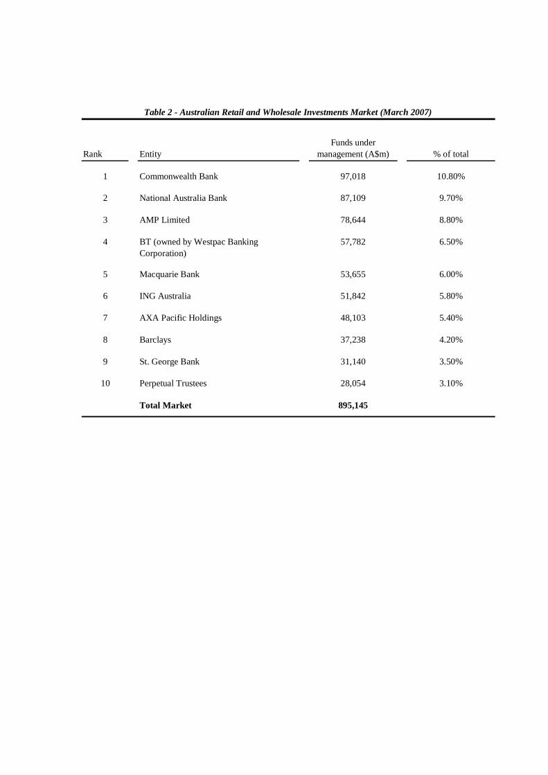
Table 2 - Australian Retail and Wholesale Investments Market (March 2007)

Rank EntityFunds under

management (A$m) % of total

1 Commonwealth Bank 97,018 10.80%

2 National Australia Bank 87,109 9.70%

3 AMP Limited 78,644 8.80%

4 BT (owned by Westpac Banking Corporation)

57,782 6.50%

5 Macquarie Bank 53,655 6.00%

6 ING Australia 51,842 5.80%

7 AXA Pacific Holdings 48,103 5.40%

8 Barclays 37,238 4.20%

9 St. George Bank 31,140 3.50%

10 Perpetual Trustees 28,054 3.10%

Total Market 895,145

24

Table 3 - Advisor location distributions

Panel A: Distribution of financial advisors by location

State No. Representatives No. Licensees Financial Centre Representatives LicenseesNSW 17,486 130 Sydney 16% 44%VIC 13,989 86 Melbourne 12% 28%QLD 10,987 1,233 Brisbane 10% 1%WA 5,306 34 Perth 10% 26%SA 4,185 13 Adelaide 17% 23%

TAS 965 1 Hobart 27% 0%ACT 867 5 Canberra 25% 40%NT 374 0 Darwin 22% 0%

Total 54,159 1,502

Panel B: Top ten postcodes by number of advisors

Postcode Region Number Postcode Region Number2000 Sydney, NSW 2,878 4217 Gold Coast, QLD 1,1953000 Melbourne, VIC 1,684 2000 Sydney, NSW 734000 Brisbane, QLD 1,066 3000 Melbourne, VIC 315000 Adelaide, SA 714 4000 Brisbane, QLD 124217 Gold Coast, QLD 622 3004 Melbourne, VIC 126000 Perth, WA 516 6000 Perth, WA 103004 Melbourne, VIC 486 6005 West Perth, WA 86005 West Perth, WA 461 2060 North Sydney, NSW 52150 Parramatta, NSW 436 3205 Sth Melbourne, VIC 54350 Gold Coast, QLD 417 6008 Subiaco, WA 5

Total 9,280 Total 1,356% of all

representatives 17% % of all licensees 90%

Panel C: Distribution of financial advisors by year of registration

Year Representatives Licensees2006 11,137 142005 11,116 192004 25,410 1422003 5,508 1,3102002 988 17Total 54,159 1,502

Representatives Licensees

Proportion of advisors in Financial Centre

25

Table 4 - Advisor Ownership Information

Panel A: The independence of financial advisors

Representatives Proportion Licensees ProportionIndependent Advisors 29,150 54% 1,272 85%Non-Independent Advisors 25,009 46% 230 15%Total 54,159 1,502

Panel B: Distribution of parent companies by primary industry

Domestic Foreign Industry Total ProportionBanking 11 15 26 18%Investment Management / Financial Services 42 23 65 45%Insurance 9 16 25 17%Other 23 4 27 19%Total 85 58 143

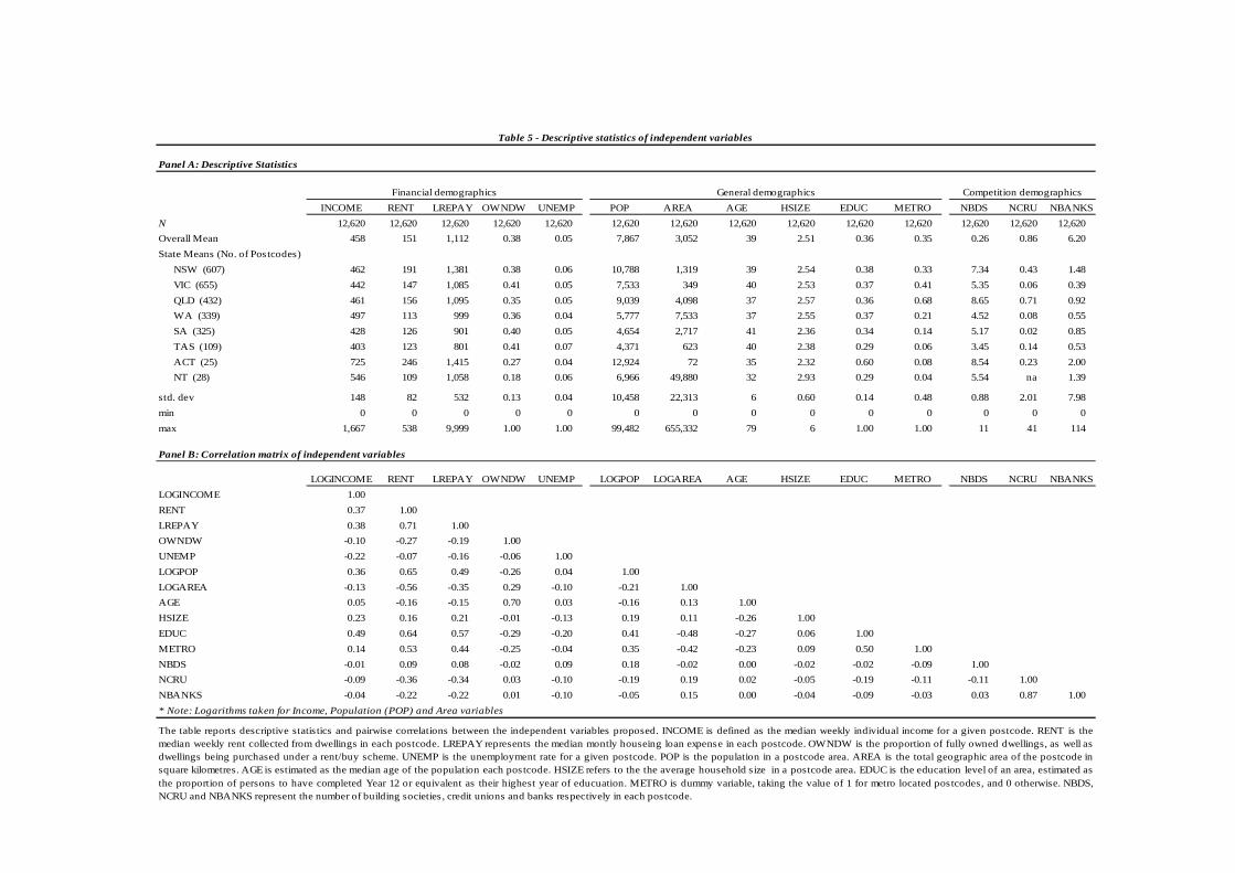
Table 5 - Descriptive statistics of independent variables

Panel A: Descriptive Statistics

INCOME RENT LREPAY OWNDW UNEMP POP AREA AGE HSIZE EDUC METRO NBDS NCRU NBANKSN 12,620 12,620 12,620 12,620 12,620 12,620 12,620 12,620 12,620 12,620 12,620 12,620 12,620 12,620Overall Mean 458 151 1,112 0.38 0.05 7,867 3,052 39 2.51 0.36 0.35 0.26 0.86 6.20State Means (No. of Postcodes)

NSW (607) 462 191 1,381 0.38 0.06 10,788 1,319 39 2.54 0.38 0.33 7.34 0.43 1.48VIC (655) 442 147 1,085 0.41 0.05 7,533 349 40 2.53 0.37 0.41 5.35 0.06 0.39QLD (432) 461 156 1,095 0.35 0.05 9,039 4,098 37 2.57 0.36 0.68 8.65 0.71 0.92WA (339) 497 113 999 0.36 0.04 5,777 7,533 37 2.55 0.37 0.21 4.52 0.08 0.55SA (325) 428 126 901 0.40 0.05 4,654 2,717 41 2.36 0.34 0.14 5.17 0.02 0.85TAS (109) 403 123 801 0.41 0.07 4,371 623 40 2.38 0.29 0.06 3.45 0.14 0.53ACT (25) 725 246 1,415 0.27 0.04 12,924 72 35 2.32 0.60 0.08 8.54 0.23 2.00NT (28) 546 109 1,058 0.18 0.06 6,966 49,880 32 2.93 0.29 0.04 5.54 na 1.39

std. dev 148 82 532 0.13 0.04 10,458 22,313 6 0.60 0.14 0.48 0.88 2.01 7.98min 0 0 0 0 0 0 0 0 0 0 0 0 0 0max 1,667 538 9,999 1.00 1.00 99,482 655,332 79 6 1.00 1.00 11 41 114

Panel B: Correlation matrix of independent variables

LOGINCOME RENT LREPAY OWNDW UNEMP LOGPOP LOGAREA AGE HSIZE EDUC METRO NBDS NCRU NBANKSLOGINCOME 1.00RENT 0.37 1.00LREPAY 0.38 0.71 1.00OWNDW -0.10 -0.27 -0.19 1.00UNEMP -0.22 -0.07 -0.16 -0.06 1.00LOGPOP 0.36 0.65 0.49 -0.26 0.04 1.00LOGAREA -0.13 -0.56 -0.35 0.29 -0.10 -0.21 1.00AGE 0.05 -0.16 -0.15 0.70 0.03 -0.16 0.13 1.00HSIZE 0.23 0.16 0.21 -0.01 -0.13 0.19 0.11 -0.26 1.00EDUC 0.49 0.64 0.57 -0.29 -0.20 0.41 -0.48 -0.27 0.06 1.00METRO 0.14 0.53 0.44 -0.25 -0.04 0.35 -0.42 -0.23 0.09 0.50 1.00NBDS -0.01 0.09 0.08 -0.02 0.09 0.18 -0.02 0.00 -0.02 -0.02 -0.09 1.00NCRU -0.09 -0.36 -0.34 0.03 -0.10 -0.19 0.19 0.02 -0.05 -0.19 -0.11 -0.11 1.00NBANKS -0.04 -0.22 -0.22 0.01 -0.10 -0.05 0.15 0.00 -0.04 -0.09 -0.03 0.03 0.87 1.00* Note: Logarithms taken for Income, Population (POP) and Area variables

General demographics Competition demographicsFinancial demographics

The table reports descriptive statis tics and pairwise correlations between the independent variables proposed. INCOME is defined as the median weekly individual income for a given postcode. RENT is themedian weekly rent collected from dwellings in each postcode. LREPAY represents the median montly houseing loan expense in each postcode. OWNDW is the proportion of fully owned dwellings, as well asdwellings being purchased under a rent/buy scheme. UNEMP is the unemployment rate for a given postcode. POP is the population in a postcode area. AREA is the total geographic area of the postcode insquare kilometres. AGE is estimated as the median age of the population each postcode. HSIZE refers to the the average household size in a postcode area. EDUC is the education level of an area, estimated asthe proportion of persons to have completed Year 12 or equivalent as their highest year of educuation. METRO is dummy variable, taking the value of 1 for metro located postcodes, and 0 otherwise. NBDS,NCRU and NBANKS represent the number of building societies , credit unions and banks respectively in each postcode.

Table 6 - Factors Affecting the Location Decisions of AFS Representatives

VariablePooled Poisson

RE Poisson

Pooled Negative Binomial

RE Negative Binomial

Pooled Logistic

RE Logistic GEE Logit

(1) (2) (3) (4) (5) (6) (7)

Constant -6.0329*** -2.5795 -3.2612 -9.2028*** -8.9755*** -7.7077** -8.9755***(2.3111) (1.9227) (2.649) (2.1063) (3.4859) (3.3939) (1.1449)

Income 0.5742** -0.378 -0.2409 0.1288 -0.1545 -0.4741 -0.1545(0.2333) (0.2374) (0.3618) (0.2826) (0.493) (0.4694) (0.1577)

Owndw 0.7492 -2.6327** -1.6206** -0.1714 -0.0258 -0.6584 -0.0258(0.5553) (1.2338) (0.6946) (0.3428) (0.6543) (0.8408) (0.395)

Unemp 2.354 -3.7565 -5.4169 -5.0098* -9.3942** -11.4558* -9.3942***(1.7475) (4.5239) (4.1024) (2.584) (4.3228) (6.4797) (1.4517)

Pop 1.0019*** 1.1041*** 1.1375*** 0.8985*** 1.3027*** 1.4273*** 1.3027***(0.0291) (0.0808) (0.0407) (0.0218) (0.0337) (0.0653) (0.0256)

Area 0.0136 -0.0473** -0.0351** -0.0014 0.0069 -0.0055 0.0069(0.0132) (0.0198) (0.0166) (0.0108) (0.018) (0.0234) (0.0121)

Age -0.0872*** -0.0054 -0.0192 0.0226*** 0.0211* 0.0266 0.0211**(0.027) (0.0188) (0.0134) (0.0071) (0.0117) (0.0206) (0.0086)

Hsize -1.0136*** -0.9571*** -1.0563*** -0.4208*** -0.6913*** -0.7772*** -0.6913***(0.0928) (0.2115) (0.1028) (0.0505) (0.0636) (0.106) (0.0533)

Metro 0.3826*** 0.3322*** 0.3366*** 0.2095*** 0.3571*** 0.4076*** 0.3571***(0.0715) (0.1009) (0.0665) (0.0464) (0.0604) (0.1107) (0.0587)

The table reports regressions of advisor locations on proposed determinants of location choice. For variable definitions, see notes to Table 5. ***, **, and * denote statisticalsignificance at the 1%, 5% and 10% level respectively, using a two tail test. Numbers in parentheses are robust standard errors adjusted for heteroskedasticity.

Variable GEE Logit GEE Logit GEE Logit

(1) (2) (2)

Constant -8.838*** -8.7018*** -7.3692***

(1.1407) (1.1409) (1.1153)

Income -0.1266 -0.1369 -0.0236

(0.1569) (0.1569) (0.1521)

Owndw 0.0024 0.0487 -0.1267

(0.3939) (0.3907) (0.3811)

Unemp -9.2598*** -10.6149*** -7.0673***

(1.4496) (1.4664) (1.4053)

Pop 1.249*** 1.1813*** 0.7926***

(0.0261) (0.0269) (0.0305)

Area -0.0033 0.0003 -0.0795***

(0.0122) (0.0122) (0.0128)

Age 0.0214** 0.0283*** 0.0303***

(0.0086) (0.0086) (0.0085)

Hsize -0.6583*** -0.6121*** -0.3164***

(0.0535) (0.0539) (0.0567)

Metro 0.3768*** 0.4529*** 0.3254***

(0.0589) (0.0596) (0.0612)

NBDS 0.2996***

(0.0379)

NCRU 0.2466***

(0.0211)

NBANKS 0.154***

(0.0067)

Table 7 - Factors affecting location choice (including competition demographics)

The table reports regressions of advisor locations on proposed determinants of location choice, after theinclusion of competition demographics. For variable names, see notes to table 5. ***, **, and * denotestatistical significance at the 1%, 5% and 10% level respectively, using a two-tail test. Numbers inparentheses are robust standard errors adjusted for heteroskedasticity.

Table 8 - Factors Affecting the Location Decisions of Foreign Affiliated AFS Representatives

VariablePooled negative Binomial

Random effects Negative Binomial Pooled Logistic

Random effects Logistic GEE Logit

(1) (2) (3) (4) (5)

Constant -11.0874** -12.9408*** -14.2241*** -14.6454*** -14.2241***(4.7825) (2.6081) (2.8265) (4.7948) (1.3631)

Income 0.5718 0.5032 0.6006 0.6133 0.6006***(0.6097) (0.3496) (0.3788) (0.6473) (0.1833)

Owndw -2.188* -0.2603 -0.1284 -0.2219 -0.1284(1.233) (0.6488) (0.5452) (0.7537) (0.499)

Unemp 2.5265 0.1362 0.361 0.488 0.361(3.3467) (3.599) (3.7582) (5.9211) (1.7434)

Pop 1.1799*** 0.9908*** 1.1433*** 1.1821*** 1.1433***(0.0697) (0.0292) (0.0341) (0.047) (0.0304)

Area -0.0718*** -0.0403** -0.0301* -0.0341 -0.0301**(0.0236) (0.0188) (0.0177) (0.0218) (0.0149)

Age -0.0078 0.0151 0.0151 0.0159 0.0151(0.0226) (0.0121) (0.0115) (0.0172) (0.0108)

Hsize -0.9025*** -0.4502*** -0.5538*** -0.5714*** -0.5538***(0.1802) (0.0798) (0.07) (0.0981) (0.0609)

Metro 0.2389** 0.0542 0.0831 0.0887 0.0831(0.0979) (0.0628) (0.0653) (0.084) (0.0652)

The table reports regression of advisor locations on the proposed determinants of location choice. The dependent variable has been limited to include only those advisorswith foreign affilications. For variable definitions, see notes to Table 5. ***, **, and * denote statistical significance at the 1%, 5% and 10% level respectively, using a two-tail test. Figures in parentheses are robust standard errors adjusted for heteroskedasticity.

Table 9 - Factors Affecting the Location Decisions of Independent and Institutionally linked AFS Representatives

Overall independent Overall institutional Banking affiliation Investment Mgmt Affiliation Insurance AffiliationVariable GEE Logit GEE Logit GEE Logit GEE Logit GEE Logit

(1) (2) (3) (4) (5)

Constant -14.1374*** -10.2128*** -7.3066*** -23.1115*** -7.5409***(1.2532) (1.1817) (1.4863) (1.8521) (1.2042)

Income 0.4372** 0.2537 -0.1636 1.7196*** -0.152(0.1716) (0.1616) (0.2046) (0.2376) (0.1651)

Owndw 0.0292 0.6997* 1.632*** 1.8152** -0.1018(0.437) (0.4243) (0.5735) (0.743) (0.4422)

Unemp -7.8984*** -3.0077** -8.2004*** 4.3691* -3.073**(1.6071) (1.5079) (2.0748) (2.2996) (1.5477)

Pop 1.3565*** 1.0657*** 1.1941*** 1.2022*** 1.0143***(0.0278) (0.0251) (0.0355) (0.0474) (0.0262)

Area -0.0107 0.0484*** 0.0429*** 0.0387* 0.0596***(0.0128) (0.0126) (0.0166) (0.0224) (0.0132)

Age 0.0354*** -0.0032 -0.0592*** 0.0008 -0.0008(0.0094) (0.0092) (0.0125) (0.0163) (0.0096)

Hsize -0.6625*** -0.6945*** -0.9419*** -0.8308*** -0.6706***(0.056) (0.0536) (0.068) (0.088) (0.0556)

Metro 0.3217*** 0.2484*** 0.3676*** 0.3307*** 0.2128***(0.06) (0.0585) (0.0734) (0.0962) (0.0612)

The table reports regression of advisor locations on the proposed determinants of location choice. For variable definitions, see notes to Table 5. ***, **, and * denotestatistical significance at the 1%, 5% and 10% level respectively, using a two-tail test. Figures in parentheses are robust standard errors adjusted for heteroskedasticity.