Locating Critical Points in 3D Vector Fields using Graphics Hardware

David Hyon Berrios ∗

University of Maryland, Baltimore County

Abstract

Calculating critical points in 3D vector fields is computationally ex-pensive, and requires parameter adjustments to maximize the num-ber and type of critical points found in a particular 3D vector field.This paper details the modifications required to execute Greene’sbisection method directly on graphics hardware, and compares theperformance of the CPU+GPU versions to the CPU only versions.

Keywords: critical points, singularities, vector fields, null points,GPGPU

1 Introduction

3D vector fields are used in computational fluid dynamics, weather,and physics simulations, among others. Because the size of the sim-ulations usually grows as the computational capabilities increase,better methods of reducing the search space within the simulationbounds becomes more important. Manual methods of searching forfeatures can no longer keep pace with the increase in the size of thedatasets. Similarly, visualizing the evolution of structural changeswithin the 3D vector fields through time becomes more difficult asthe 3D vector fields become larger (higher resolution, both temporaland spatial) and the simulations become longer (more timesteps).

An example can illustrate the difficulty of searching a 3D vectorfield for a particular feature. Suppose a user wanted to locate atornado in a weather simulation that spanned the entire earth. Nor-mally, thresholds could be used to locate regions where the windspeed was higher than the threshold. Although the wind speed is agood heuristic for locating tornadoes, it does not uniquely identifytheir locations. Hurricanes can also have strong winds, but theirbehaviors and characteristics are vastly different. Alternatively, theeffort of finding this tornado in both the space of each individualtimestep, and across multiple timesteps, can be offset by using crit-ical points. A tornado exists as a vortex within a 3D vector field,with a sink or source at its base. The point at which the vectorfield vanishes, a critical point, can be used to find a location ineach timestep that could possibly show a tornado. This narrows thesearch space, both in time and space.

With the exception of a few algorithms [Globus et al. 1991; Parnellet al. 1996], the algorithms used to calculate critical points share asimilar trait that make them perfect candidates for modern parallelarchitectures: the operations applied to each sub-volume within asimulation can be performed independently of all other operationson other sub-volumes. Modern graphics hardware has been shownto accelerate calculations for parallel problems, and conventionalparallel machines have been used to accelerate critical point calcu-lations [Gerndt et al. 2006]. No work has been done to acceleratethe calculation of critical points using graphics hardware.

The rest of the paper is presented as follows. The background sec-tion summarizes the information related to vector fields and crit-ical points. The related work section is split into the two sub-sections used in this work: an overview of Greene’s bisectionmethod [Greene 1992], and methods of accelerating problems usingparallel machines, including graphics hardware. The implementa-tion section details the changes required to Greene’s bisection to

∗e-mail: david.berrios@umbc.edu

execute on modern graphics hardware. Finally, the results of bench-marks are presented, comparing the CPU version of the algorithmto a CPU+GPU version.

2 Background

This section provides background information on vector fields, crit-ical points, and algorithms used to locate the critical points. Thevector fields are created either from simulations, or from derivedcalculations of scalar fields.

2.1 Vector Fields

Figure 1: An example of a 2D vector field

A vector field consists of a grid of positions, with each positionhaving one or more vectors. An example 2D vector field is shownin Figure 1. Vector fields are generally used in physics-based sim-ulations from complex parallel codes. A scalar field is similar to avector field, but with scalars associated with the positions insteadof vectors. By calculating the gradient or some other function thatyields a vector, a derived vector field can be created from scalarfields. Since the vector fields themselves share common propertiesacross disciplines, algorithms applied to vector fields will benefitall domains that use vector fields. So, for example, visualizationtechniques created for and applied to computational fluid dynamicssimulations can be applied and will benefit space weather simula-tions and vice versa. A more thorough description of vector fields isgiven by Morse and Feshbach [1953], with applications to physicsproblems.

2.2 Critical Points

Critical points are positions within a vector field where the vectorfield vanishes. More detailed information about critical points canbe found in the books by Arnold [1992; 1993], and Palais and Terng[1988]. Finding these positions within a vector field is importantbecause it allows the exploration of a vector field by extracting fea-tures from the vector field that exist near or are characterized by thecritical points. These features are enough to characterize the globaltopology of the vector field, allowing less information to be dis-played. When dealing with simulation data from complex parallelcodes, minimizing the search space helps the exploration process.

The topological degree, also called the Poincare index, is a math-ematical property from the Poincare-Hopf theorem. It is used as avalue to determine whether a critical point exists within some vol-ume of space. It represents the number of times the angle (2D)or solid angle (3D) of the vectors at the boundary of a closed lineor volume, covers a unit circle (2D) or unit sphere (3D). The vol-ume used is dependent on the algorithm, but normally a cube is

used, since it is topologically the same as a sphere, and is non-overlapping. The two terms, degree and index, are used inter-changeably. A critical point having an index of 1 represents asource, while a critical point having an index of -1 represents asink. Higher order critical points are those critical points having anindex whose magnitude is greater than 1.

3 Related Work

Several algorithms can be used to calculate critical points in vectorfields; Greene’s bisection method was chosen because of its easeof implementation, and quality of the results. Greene’s bisectionalgorithm, along with other methods of calculating critical pointsare discussed for completeness.

In 1992, Greene published the first method for locating first-ordercritical points (i.e., index is -1 or 1) in 3D vector fields using thetopological degree. A previous algorithm used a similar initialmethod [Globus et al. 1991], but found the nulls by using Newton-Raphson iteration to converge to the solution for each cell; it re-quired an initial guess and did not always converge to a solution.Greene introduced the concept of the topological degree of a vol-ume in a 3D vector field. The topological degree is the Poincareindex, evaluated using surface vector values of a sub-volume withina 3D vector field. Greene’s algorithm evaluates sub-cubes within a3D vector field. For each face of a cube, a diagonal line is createdthat separates the face into two triangles. The vectors at the verticesof each triangle are projected onto a unit sphere. The solid angleformed by this projection is added or subtracted to a global valuefor a given sub-volume, depending on the sign of the cross productof two of the vectors, dotted with the third (essentially, either in-ward or outward). In particular, Greene focused on locating criticalpoints with a topological degree of 1 or -1, which are critical pointswith a degree of one. This was also a limitation of the algorithm,since it could not find higher-order critical points (those points withdegrees higher than one).

Schaeuermann et al. [1997] created an algorithm, using the nota-tions from clifford algebra, to find singularities having a higher-order, but it only applied to 2D vector fields. Their work alsoincluded diagrams showing higher-order critical points in the 2Dcase.

Mann and Rockwood [2002] extended the work by Schauermann etal., and introduced an algorithm to calculate singularities of higher-order than previously possible for higher dimensions. Singularities,in this case, are equivalent to critical points. They utilize multivec-tors and operators from geometric algebra, using an implementationprovided by the work of Fonijne [2006], to calculate and evaluatethe topological degree of a sub-volume. For each face of a sub-cube, a grid is created and vectors are interpolated onto the grid,using trilinear interpolation of the vectors at the corners. The con-tributions of the trivectors and bivectors from each face are added tocalculate the topological degree. As in Greene’s bisection method,the cubes that have a non-zero index are bisected and the algorithmrepeats. Because Mann and Rockwood’s method projects the vec-tors onto each face of the cube, the algorithm locates singularitiesthat exist only because of the projection of the vectors onto thefaces, but some of those singularities do not exist in the originalvector field. They use a heuristic to help eliminate these false sin-gularities. Useful references for geometric algebra and its appli-cations to computer science are included in books by Dorst et al.[2007], and Vince [2008].

Furuheim wrote a masters thesis that compares an analyticalmethod to Greene’s bisection method and demonstrates new meth-ods of visualizing 3D vector fields using the calculated criticalpoints [2008]. Furuheim’s algorithm locates more first order critical

points than Greene’s bisection method, but like Greene’s algorithm,it cannot find critical points of higher degree than one. This workdemonstrates that Greene’s algorithm is still comparable to newertechniques.

All current algorithms used to calculate critical points in vectorfields rely on the Poincare index and all bisect the volume to narrowthe search for the true location. The difference exists in how theysetup the calculations to approximate the index.

4 Implementation

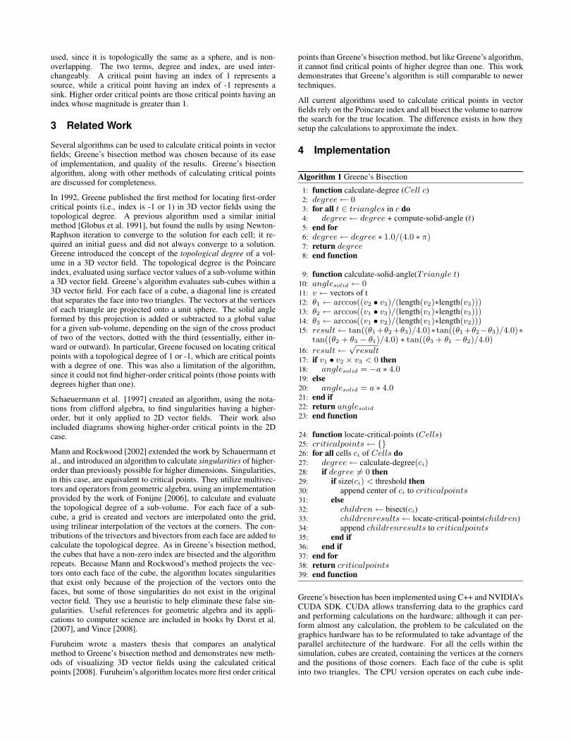
Algorithm 1 Greene’s Bisection

1: function calculate-degree (Cell c)2: degree← 03: for all t ∈ triangles in c do4: degree← degree + compute-solid-angle (t)5: end for6: degree← degree ∗ 1.0/(4.0 ∗ π)7: return degree8: end function

9: function calculate-solid-angle(Triangle t)10: anglesolid ← 011: v ← vectors of t12: θ1 ← arccos((v2 • v3)/(length(v2)∗length(v3)))13: θ2 ← arccos((v1 • v3)/(length(v1)∗length(v3)))14: θ3 ← arccos((v1 • v2)/(length(v1)∗length(v2)))15: result← tan((θ1+θ2+θ3)/4.0)∗tan((θ1+θ2−θ3)/4.0)∗

tan((θ2 + θ3 − θ1)/4.0) ∗ tan((θ3 + θ1 − θ2)/4.0)

16: result←√result

17: if v1 • v2 × v3 < 0 then18: anglesolid = −a ∗ 4.019: else20: anglesolid = a ∗ 4.021: end if22: return anglesolid

23: end function

24: function locate-critical-points (Cells)25: criticalpoints← {}26: for all cells ci of Cells do27: degree← calculate-degree(ci)28: if degree 6= 0 then29: if size(ci) < threshold then30: append center of ci to criticalpoints31: else32: children← bisect(ci)33: childrenresults← locate-critical-points(children)34: append childrenresults to criticalpoints35: end if36: end if37: end for38: return criticalpoints39: end function

Greene’s bisection has been implemented using C++ and NVIDIA’sCUDA SDK. CUDA allows transferring data to the graphics cardand performing calculations on the hardware; although it can per-form almost any calculation, the problem to be calculated on thegraphics hardware has to be reformulated to take advantage of theparallel architecture of the hardware. For all the cells within thesimulation, cubes are created, containing the vertices at the cornersand the positions of those corners. Each face of the cube is splitinto two triangles. The CPU version operates on each cube inde-

pendently of all other cubes, while the GPU version operates on alltriangles independently of all other triangles.

NVIDIA hardware can operate on 32 thread chunks, called warps,at a time. The number of threads should be multiples of 16 or 32to maximize the number of calculations performed. Blocks aregroups of threads that share memory. When threads in one blockrequire access to data in memory (requiring a significant numberof clock cycles), the graphics hardware can swap that block for an-other one and continue operating. As a result, the more blocks thatare available to operate on a problem, the more the built-in sched-uler can hide the memory latencies. For the two graphics cardsbenchmarked, the 8600M GT and the 8800 GT, the warp size is32. To maximize the parallelism, each warp should have 32 threadsto execute. See the CUDA programming guide[NVIDIA 2008] formore technical aspects for programming on NVIDIA hardware .

Each cube created from the data was separated into twelve triangles(two triangles per face, six faces). The grid was specified as 512blocks × 32 threads per block for a total grid size of 16384. Eachthread operated on an individual triangle, performing the series ofoperations listed in function calculate-solid-angle. Whenever pos-sible, faster, less accurate single precision versions of operationswere used. These include tanf, and fdividef. For each mem-ory transfer to the graphics device, 16384 triangles are sent, andthe results are then inspected. The candidate cells are created fromthe cells having a non-zero index; these cells are bisected into eightchildren, and added to a candidate cells list. When the initial pass iscomplete, the candidate cells are then processed and the algorithmcontinues. The results are returned when the cells being inspectedare smaller than a threshold size.

Two versions of the GPU accelerated Greene’s bisection were cre-ated: one that performed all the triangle calculations on graphicshardware, and one that only performed the initial scan on graphicshardware. In most cases, the number of candidate cells after thefirst pass is significantly less than the number of total cells. Veryrarely will the number of critical points equal the number of cells inthe 3D vector field. By eliminating the necessary overhead of trans-ferring a smaller number of cells after each pass, the performanceis increased.

5 Results

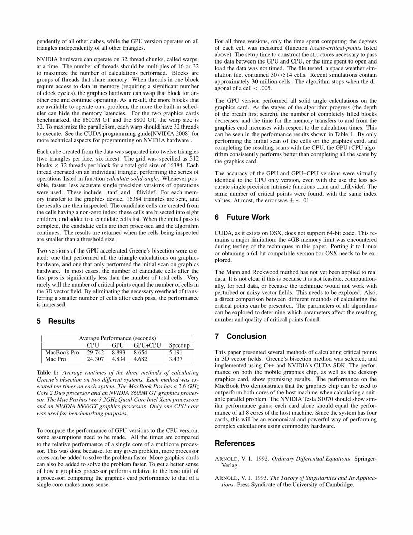
Average Performance (seconds)CPU GPU GPU+CPU Speedup

MacBook Pro 29.742 8.893 8.654 5.191Mac Pro 24.307 4.834 4.682 3.437

Table 1: Average runtimes of the three methods of calculatingGreene’s bisection on two different systems. Each method was ex-ecuted ten times on each system. The MacBook Pro has a 2.6 GHzCore 2 Duo processor and an NVIDIA 8600M GT graphics proces-sor. The Mac Pro has two 3.2GHz Quad-Core Intel Xeon processorsand an NVIDIA 8800GT graphics processor. Only one CPU corewas used for benchmarking purposes.

To compare the performance of GPU versions to the CPU version,some assumptions need to be made. All the times are comparedto the relative performance of a single core of a multicore proces-sor. This was done because, for any given problem, more processorcores can be added to solve the problem faster. More graphics cardscan also be added to solve the problem faster. To get a better senseof how a graphics processor performs relative to the base unit ofa processor, comparing the graphics card performance to that of asingle core makes more sense.

For all three versions, only the time spent computing the degreesof each cell was measured (function locate-critical-points listedabove). The setup time to construct the structures necessary to passthe data between the GPU and CPU, or the time spent to open andload the data was not timed. The file tested, a space weather sim-ulation file, contained 3077514 cells. Recent simulations containapproximately 30 million cells. The algorithm stops when the di-agonal of a cell < .005.

The GPU version performed all solid angle calculations on thegraphics card. As the stages of the algorithm progress (the depthof the breath first search), the number of completely filled blocksdecreases, and the time for the memory transfers to and from thegraphics card increases with respect to the calculation times. Thiscan be seen in the performance results shown in Table 1. By onlyperforming the initial scan of the cells on the graphics card, andcompleting the resulting scans with the CPU, the GPU+CPU algo-rithm consistently performs better than completing all the scans bythe graphics card.

The accuracy of the GPU and GPU+CPU versions were virtuallyidentical to the CPU only version, even with the use the less ac-curate single precision intrinsic functions tan and fdividef. Thesame number of critical points were found, with the same indexvalues. At most, the error was ± ∼ .01.

6 Future Work

CUDA, as it exists on OSX, does not support 64-bit code. This re-mains a major limitation; the 4GB memory limit was encounteredduring testing of the techniques in this paper. Porting it to Linuxor obtaining a 64-bit compatible version for OSX needs to be ex-plored.

The Mann and Rockwood method has not yet been applied to realdata. It is not clear if this is because it is not feasible, computation-ally, for real data, or because the technique would not work withperturbed or noisy vector fields. This needs to be explored. Also,a direct comparison between different methods of calculating thecritical points can be presented. The parameters of all algorithmscan be explored to determine which parameters affect the resultingnumber and quality of critical points found.

7 Conclusion

This paper presented several methods of calculating critical pointsin 3D vector fields. Greene’s bisection method was selected, andimplemented using C++ and NVIDIA’s CUDA SDK. The perfor-mance on both the mobile graphics chip, as well as the desktopgraphics card, show promising results. The performance on theMacBook Pro demonstrates that the graphics chip can be used tooutperform both cores of the host machine when calculating a suit-able parallel problem. The NVIDIA Tesla S1070 should show sim-ilar performance gains; each card alone should equal the perfor-mance of all 8 cores of the host machine. Since the system has fourcards, this will be an economical and powerful way of performingcomplex calculations using commodity hardware.

References

ARNOLD, V. I. 1992. Ordinary Differential Equations. Springer-Verlag.

ARNOLD, V. I. 1993. The Theory of Singularities and Its Applica-tions. Press Syndicate of the University of Cambridge.

Figure 2: Performance of the different methods of calculating the critical points using Greene’s bisection. The CPU times represent the timeit takes for one core to complete the calculations. The MacBook Pro has an NVIDIA 8600M GT graphics card, and the Mac Pro has anNVIDIA 8800GT graphics card. The GPU times represent the time it takes for the respective graphics cards to complete the calculations.

(a) A fluxrope on the day-side of a global magneto-sphere simulation.

(b) A single fieldline that characterizes the boundarybetween three different topologies.

Figure 3: Visualizations showing a feature that can be found using critical points.

DORST, L., FONTIJNE, D., AND MANN, S. 2007. GeometricAlgebra for Computer Science: An Object-Oriented Approachto Geometry. Morgan Kaufmann Publishers.

FONTIJNE, D. 2006. Gaigen 2:: a geometric algebra implemen-tation generator. In GPCE ’06: Proceedings of the 5th interna-tional conference on Generative programming and componentengineering, ACM, New York, NY, USA, 141–150.

FURUHEIM, K. 2008. Classification and Visualization of CriticalPoints in 3D Vector Fields. Master’s thesis, University of Oslo.

GERNDT, A., SARHOLZ, S., WOLTER, M., MEY, D. A.,BISCHOF, C., AND KUHLEN, T. 2006. Nested OpenMP forefficient computation of 3D critical points in multi-block CFDdatasets. In SC ’06: Proceedings of the 2006 ACM/IEEE confer-ence on Supercomputing, ACM, New York, NY, USA, 93.

GLOBUS, A., LEVIT, C., AND LASINSKI, T. 1991. A tool forvisualizing the topology of three-dimensional vector fields. InVIS ’91: Proceedings of the 2nd conference on Visualization ’91,IEEE Computer Society Press, Los Alamitos, CA, USA, 33–40.

GREENE, J. M. 1992. Locating three-dimensional roots by a bisec-tion method. Journal of Computational Physics 98, 2, 194–198.

MANN, S., AND ROCKWOOD, A. 2002. Computing singularitiesof 3D vector fields with geometric algebra. In VIS ’02: Pro-ceedings of the conference on Visualization ’02, IEEE ComputerSociety, Washington, DC, USA, 283–290.

MORSE, P. M., AND FESHBACH, H. 1953. Methods of TheoreticalPhysics: Part 1. McGraw-Hill Book Company, Inc.

NVIDIA. 2008. NVIDIA CUDA Compute Unified Device Archi-tecture Programming Guide. NVIDIA.

PALAIS, R. S., AND TERNG, C. 1988. Critical Point Theory andSubmanifold Geometry. Springer-Verlag.

PARNELL, C. E., SMITH, J. M., NEUKIRCH, T., AND PRIEST,E. R. 1996. The structure of three-dimensional magnetic neutralpoints. Physics of Plasmas 3 (Mar.), 759–770.

SCHEUERMANN, G., HAGEN, H., KRUGER, H., MENZEL, M.,AND ROCKWOOD, A. 1997. Visualization of higher order sin-gularities in vector fields. In VIS ’97: Proceedings of the 8thconference on Visualization ’97, IEEE Computer Society Press,Los Alamitos, CA, USA, 67–74.

VINCE, J. 2008. Geometric Algebra for Computer Graphics.Springer.