localization and coherence in nonintegrable...
TRANSCRIPT
Physica D 184 (2003) 162–191
Localization and coherence in nonintegrable systems
Benno Rumpfa,∗, Alan C. Newellba Max-Planck-Institut für Physik Komplexer Systeme, Nöthnitzer Straße 38, 01187 Dresden, Germany
b Mathematics Department, University of Arizona, 617 North Santa Rita, Tucson, AZ 85721, USA
Abstract
We study the irreversible dynamics of nonlinear, nonintegrable Hamiltonian oscillator chains approaching their statisticalasymptotic states. In systems constrained by more than one conserved quantity, the partitioning of the conserved quantitiesleads naturally to localized and coherent structures. If the phase space is compact, the final equilibrium state is governedby entropy maximization and the coherent structures are stable lumps. In systems where the phase space is not compact,the coherent structures can be collapsed, represented in phase space by a heteroclinic connection of some unstable saddle toinfinity.© 2003 Elsevier B.V. All rights reserved.
Keywords:Localized structures; Statistical physics
1. Introduction
The formation of coherent structures by a continuing self-focusing process is a widespread phenomenon indispersive nonlinear wave systems. As a result of this process, high peaks of some physical field emerge from alow-amplitude noisy background. For optical waves in Kerr-nonlinear media this results in a self-enhanced increaseof light intensity in a small sector of a laser beam while the intensity in the neighborhood of this bright spot decreases[1]. Related phenomena occur in diverse systems from hydrodynamics to collapsing Langmuir waves in a plasma[2] and in numerical algorithms for partial differential equations[3,4].
A common feature of the wave dynamics of these systems is the comparable strength of the dispersion andthe nonlinearity. But, self-focusing phenomena are radically different in integrable and nonintegrable systems. Inintegrable systems[5], the peaks appear and disappear in a quasiperiodic manner reflecting the phase space structureof nested tori. This behavior is usually encountered on time scales that are short enough so that generic nonintegrablecontributions to the dynamics may be neglected. Significant changes occur on time scales where the nonintegrabilityis relevant[6,7]. The solution’s shape becomes more irregular[8–11]and the periodic breathing of the peaks turnsinto a more persistent state. These peaks can merge into stronger ones while radiating low-amplitude waves. Theirreversible character of the system becomes apparent and its behavior is driven by statistical mechanics[12–14]asthe solution’s trajectory tries to explore more of the available phase space. As it does this, it must, at the same time,
∗ Corresponding author.E-mail address:[email protected] (B. Rumpf).
0167-2789/$ – see front matter © 2003 Elsevier B.V. All rights reserved.doi:10.1016/S0167-2789(03)00220-3
B. Rumpf, A.C. Newell / Physica D 184 (2003) 162–191 163
respect the preservation of conserved quantities. The phase space shell of constant conserved quantities determinesthe system’s most favorable macrostate and the resulting dynamics can lead to a local gathering of the amplitudewhile the system explores the phase space shell. We will see in situations with more than one conserved quantitythat the spatial structure of the state which is statistically preferred now contains coherent peaks. If the phase spaceis compact, these peaks can be local, time independent and stable. If the phase space is not compact, the peaks canbe collapsing filaments which produce singularities.
In this paper we study three systems which typify the focusing behavior observed in nonintegrable Hamiltoniansystems with more than one conserved quantity, namely the Landau–Lifshitz equation for a classical Heisenbergspin chain, various versions of the discrete nonlinear Schrödinger (DNLS) equation, and a leapfrog-discretizationof the Korteweg–de Vries (KdV) equation. Various modifications of these systems help to identify the role of theconserved quantities in the formation of coherent structures. The spatial discreteness of all these systems avoidsfluctuations on infinitesimal scales.
The first case study investigates the Landau–Lifshitz equation for the classical spin chain in one spatial dimension.We study the long time behavior of those configurations in which most spins are close to the north pole. Thetwo conserved quantities are the energy and the magnetic moment. Almost constant states undergo a series ofmodulational instabilities and the system begins to oscillate as if it were integrable. Nonintegrability, however, leadsto nonrecurrence as localized peaks appear which merge from time to time leading to even larger peaks and radiatingsome energy. The phase space is compact, and one can compute to good accuracy the thermodynamic potentialsof the system by separating the low-amplitude spin-waves and the strongly nonlinear components. Depending onthe initial value of the energy and the magnetization, entropy maximization leads to a state where some of themagnetization must be put into local structures bounded by domain walls for which the spin of each containedlattice point is close to the south pole. Numerical simulations very clearly support our simple analytical predictionswhich are based on thermodynamic considerations.
A close relative of the Heisenberg spin chain is found by taking the small amplitude limit where all spins are closeto the north pole. Deviations are described by the focusing nonlinear Schrödinger equation. A similar dynamics isobserved. In this study, we can also investigate the effects of exact integrability by using the Ablowitz–Ladik algo-rithm [15]. In these simulations, we find no irreversible behavior, no peak fusion, no relaxation, only quasiperiodicbehavior. Likewise, we get qualitatively different results if we take a model which breaks the rotational symmetryand because of this the particle number is no longer conserved. As a consequence it is not necessary for the systemto develop coherent structures in order to maximize its entropy as it no longer has to be concerned about the secondconstant of motion when its trajectory explores the accessible phase space.
The last case study concerns the leapfrog algorithm for the numerical integration of the KdV equation. It wasobserved in previous works[3,4] that the leapfrog algorithm for the KdV equation always develops singularities.After (usually) a very long time, the amplitudes in some local neighborhood rapidly diverges. We demonstrate thatthis collapse again takes on an organized coherent form.
How and why does the system develop such local objects? The reason is again statistical. At an early stage,one can again observe the gathering of one of the conserved quantities in coherent structures. The system’s phasespace is not compact, however, so that a strong nonequilibrium process prevails finally. We find a rapidly growinglocalized ‘monster’ solution (so called because of its likeness in shape to the Loch Ness monster) that has a canonicalstructure. This solution can originate from coherent structures or, most frequently, from a long wave instability ofthe low-amplitude noisy background. We discuss the similarity of this process to the collapse behavior of thetwo-dimensional focusing nonlinear Schrödinger equation, where the conservation laws necessitate a net inverseparticle flux to small wavenumbers.
This paper is arranged as follows. InSection 2, we present the Landau–Lifshitz equation, the DNLS equationand the leapfrog-discretization of the KdV equation and discuss some of their properties. InSection 3we present

164 B. Rumpf, A.C. Newell / Physica D 184 (2003) 162–191
numerical studies of these equations. In particular, we study thermodynamic quantities during the focusing process.Their significance is also demonstrated by discussing modified equations with either more or with fewer conservedquantities as well as an equation of defocusing type. InSection 4we will give a statistical interpretation of thenumerical findings. By computing the thermodynamic potentials of the spin system, we find the connections betweenglobal features of the pattern and the conserved quantities. Macroscopic properties of the final state are computed.The discretized KdV equation has no such state of thermal equilibrium. We identify the rapid divergence of theamplitudes with the exploration of the noncompact phase space shell and we suggest that there is much similaritybetween this behavior and the condensation and collapse behavior seen in the focusing nonlinear Schrödingerequation.
Figures of similar contents are grouped together and their order sometimes deviates from the sequence of theirreferences in the text.
2. Nonintegrable systems with constraints
2.1. Time-continuous systems
2.1.1. The Landau–Lifshitz equationThe anisotropic Heisenberg spin chain is particularly suitable for the study of self-focusing phenomena. This
system contains the generic properties of equations of nonlinear Schrödinger type that lead to self-focusing and itis easy to investigate from the statistical point of view. The Landau–Lifshitz equation[16]
Sn = Sn × (J(Sn−1 + Sn+1) + Snzez), (1)
is a classical approximation of the dynamics of magnetic momentsSn = (Sxn, Syn, Szn) at lattice sitesn. Sn isperpendicular toSn. Therefore the moduli of the spin vectors are conserved and one may set|Sn| = 1. Thephase space of a chain ofN spins is a product ofN such spheres.Sz the component ofS along the rotationalsymmetry axis. The northern and southern hemispheres are equivalent since(1) is invariant under the transformation(Sxn, Syn, Szn) → (−Sxn, Syn,−Szn).
There are two trivial homogeneous equilibrium states where all the spins point either to the north poleSz = 1 orto the south poleSz = −1. Throughout this paper we only consider solutions where most of the spins are close tothe north pole.
2.1.2. The DNLS equationThe long-wavelength dynamics of spins which deviate slightly from the north poleSz = 1 is given by the focusing
DNLS equation
iφn = J(φn+1 + φn−1 − 2φn) + 2|φn|2φn (2)
for small values of the complex amplitudeφ = (Sx + iSy)/(1+Sz). The spin chain may thus be regarded as a DNLSwhich is modified by higher order terms. The north pole corresponds toφ = 0 while the south pole corresponds toan infinite amplitude.
2.1.3. Integrals of motionThe spin chain and the DNLS equation each have two conserved quantities:
1. The Hamiltonian of the DNLS equationH = ∑n J(2φnφ
∗n − φnφ
∗n+1 − φ∗
nφn+1) − |φn|4 is again obtained asthe lowest order of the Hamiltonian of the spin chainH = HJ +Ha = ∑
n J(1 − SnSn+1) + (1 − S2zn)/2. The

B. Rumpf, A.C. Newell / Physica D 184 (2003) 162–191 165
first contribution is a Heisenberg exchange coupling which is minimal for homogeneous solutions. The secondpart is an anisotropic energy that has minima at the polesSz = ±1 and is maximal at the equatorSz = 0. Thestationary spin-up or spin-down solutions are the absolute energy minima. Fluctuations about these ground statesgive energy contributions per lattice site of the order of|Sx + iSy|2. Similarly, small fluctuations near by theequilibrium stateφ = 0 of the DNLS contribute a coupling energy proportional to|φ|2. In contrast to the southpole state of the spin system, the energy of a solutionφ → ∞ in the DNLS goes to minus infinity as−|φ|4.
2. The second conserved quantity of each system, the total magnetizationM = ∑n Szn of the spin chain and the
modulus-square norm (‘particle number’)∑
n |φn|2 of the DNLS are related to the system’s rotational symmetry.The superposition of the Hamiltonian and this integral of motion yields a Hamiltonian in a rotating frame system.The negative magnetizationN −M = ∑
(1− Szn) ≈ ∑ |Sxn + iSyn|2/2 corresponds to the particle number ofthe DNLS in the lowest order in amplitude. This ‘particle number’ of the spin chain is zero for the north polesolution and it is two per lattice site for the south pole solution. In the DNLS, the particle number diverges forthe state|φ| → ∞.
In order to contrast the generic behavior of such systems with those of (a) integrable systems and (b) systemsnot constrained by a second conservation law, we also consider two modified equations of motion. The first is theintegrable Ablowitz–Ladik discretization of the one-dimensional nonlinear Schrödinger equation[15]. The secondis an equation where the second integral is destroyed by a symmetry breaking field.
Low-energetic solutions just above the ground states can be characterized by the ratio of the two integrals ofmotion, i.e. the energy per particle. This reveals a major difference between the spin chain and the DNLS. Forfluctuations near the north pole or nearφ = 0, the particle number is of the order of the energy so that this ratio isof order one for both systems. Spin-fluctuations near the south pole have the same energy but the second conservedquantity (‘particle number’) is much higher so that the energy per particle is proportional to|Sx + iSy|2 and muchless than 1. Thus the spin chain has two states with low energies per lattice site, one (Sz ≈ 1) with a higher energy perparticle and one (Sz ≈ −1) with a low positive energy per particle. This well-defined condensate state of low-energyand high particle density is a major advantage of the spin chain.
In contrast, for infinitely high-amplitude solutions of the DNLS that correspond toSz ≈ −1 solutions of the spinchain both the energy and the particle density go to infinity. The energy per particle diverges proportional to−|φ|2.
2.2. Time-discretized equation of motion
2.2.1. The leapfrog-discretization of the KdV equationThe system of finite difference equations
um+1(n) = vm(n) + τ(um(n + 2) − 2um(n + 1) + 2um(n − 1) − um(n − 2)
− 2(um(n + 1) + um(n) + um(n − 1))(um(n + 1) − um(n − 1))), (3a)
vm+1(n) = um(n), (3b)
is a leapfrog-type discretization in space and time of the completely integrable KdV equationu = uxxx−6uux for thereal amplitudeu(x, t). The leapfrog-discretization is characterized by a central difference∂u/∂t → (um+1−um−1).The factorτ of the spatial derivative is the time step-size. The precursorum−1 is identified with the additionalvariablevm on the right side of the first equation. This scheme allows the simulation of the partial differentialequation avoiding the amplitude dissipation that occurs in methods with numerical viscosity. The termum(n+2)−2um(n + 1) + 2um(n − 1) − um(n − 2) is the standard discretization ofuxxx. The discretization ofuux was first

166 B. Rumpf, A.C. Newell / Physica D 184 (2003) 162–191
suggested by Zabusky and Kruskal[17]. It involves a central difference in spaceum(n+1)−um(n−1) and replacesu by the average(um(n + 1) + um(n) + um(n − 1))/3.
This discretization suppresses fast-acting nonlinear instabilities. Discretizations that do not retain some of theoriginal conservation laws lead to fast-acting instabilities, since single modes diverge rapidly. For instance, themode with the wavenumberk = 2π/3 is driven by the nonlinear part of conventional discretizations of the KdVequation. In contrast, this mode is an exact solution of(3). Linear instabilities of the zero-solution can be avoidedby a sufficiently small step-sizeτ < 2/(3
√3).
2.2.2. Integrals of motionThe special feature of the spatial discretization(3) is that it preserves some of the original conserved quantities:
1. 〈uv〉 = ∑n um(n)vm(n) = const. corresponds to the conserved quantity
∫u2 dx (‘energy’ for shallow water
waves) in the original KdV equation. The modulus-square norm〈u2 + v2〉 = ∑n um(n)2 + vm(n)2 is not
conserved.2. 〈u〉 = ∑
n u2m(n) = ∑n v2m+1(n) and〈v〉 = ∑
n v2m(n) = ∑n u2m+1(n) correspond to
∫udx (‘mass’ for
shallow water waves).
3. Numerical studies
We examine the formation of coherent structures numerically in various versions of the spin chain and the DNLSequation as well as the leapfrog integration scheme for the KdV equation. A typical scenario for the spin chainsuggests that the final state mainly depends on the amount of the two conserved quantities provided by the initialconditions. Simulations of various modifications of the DNLS with either more of less integrals of motion clarifysome more general conditions for this behavior. The simulations of the differential equations apply an Adams routineto a chain of 512 (and occasionally 4096) oscillators with periodic boundary conditions.
3.1. Dynamics of the spin chain
3.1.1. Benjamin–Feir instability and reversible dynamicsPlane wave solutions of the nonlinear Schrödinger equation are Benjamin–Feir unstable so that self-focusing is
initiated by long-wavelength modulations. Similarly, spin-wave solutions of the Heisenberg spin chain are unstableunder long-wavelength perturbations. For instance, the homogeneously magnetized solutionSn = S (Fig. 1a) thatprocesses about the symmetry axisez with the frequencyω = Sz is most unstable under perturbations with the
wavenumberk =√
1 − S2z /J .
As a result of this instability, small perturbations lead to spatially periodic humps of spins approaching the equatorwhile most of the spins come closer to the north pole (Fig. 1b). The trajectory is close to a homoclinic orbit sothat the solution returns to the almost homogeneous state after reaching the maximum amplitude.Fig. 2a shows theprofile of thez-magnetization in space and time for this solution which is almost periodic in space and time.Fig. 3ashows the pattern of peaks (the sites of the spins that differ most from the north pole) as a function of time;Fig. 2ais related to box (α) of Fig. 3a. Equidistant humps emerge and disappear periodically in time fort < 200.
3.1.2. Merging of peaks and irreversible dynamicsThe spatially periodic solution arising from the Benjamin–Feir instability is itself phase-unstable. As a result, the
periodic pattern with the wavelength of the initial periodic mode becomes modulated on an even larger length scale

B. Rumpf, A.C. Newell / Physica D 184 (2003) 162–191 167
(a)
(b)
(d)
(c)
Fig. 1. Sketch of the spins for the (a) spatially homogeneous solution, (b) spatially periodic solution resulting from a Benjamin–Feir instability,(c) humps moving towards each other merging into compound peaks of spins pointing down (d).
so that the gaps between the initially equidistant humps start to vary (Fig. 1c). Fig. 3a shows tiny variations of thedistances between the humps as the humps start to move att ≈ 60.
The most important phenomenon following the phase instabilities is the formation of coherent structures throughmergings of peaks. Neighboring humps approaching each other finally merge into single peaks radiating smallfluctuations.Fig. 2b shows the profile of the magnetization during the fusion of humps of box (β) in Fig. 3a.The original periodic solution is smooth, but the compound peak resulting from the merging has an irregular shapeinvolving huge gradients both in space and in time. Its amplitude oscillates irregularly in time, but unlike the originalperiodic solution, it does not vanish any more completely. Even those humps that are situated remotely from the firstmerging processes become more persistent in time immediately so that they are traced by continuous lines inFig. 3a.
Subsequently, more humps fusing into compound peaks increase the average distance between neighboring peaks.The resulting compound peaks again merge with primary humps and with other compound peaks forming evenstronger peaks (see point (γ) in Fig. 3b with the magnetization profile ofFig. 2c).
3.1.3. Final equilibrium stateThe increasingly high-amplitude of the compound peaks enables some spins to overcome the energy barrier of
the equator and to flip to the southern hemisphere (Fig. 1d). Fig. 3b shows that after 2× 10⁵ time steps all peakshave merged into six down-magnetized domains that each consist of two or three lattice points. These peaks withSz ≈ −1 are embedded in a disordered state where the spins deviate only slightly from the north poleSz = 1. Thefinal state is a two domain pattern where most of the spins are accumulated in huge up-magnetized domains while afew spins condense to small down-magnetized domains. The domain of the spin-wave fluctuations near to the northpole in the final state remains persistent even if the spin-down xenocrysts are removed artificially by flipping thedown-spins up asSz → |Sz|.
3.1.4. Transfer of energyThe transition from the almost regular dynamics to the irreversible process during the merging of peaks is reflected
in the share of the total energy of the two parts of the Hamiltonian. The coupling energyHJ = ∑(1 − SnSn+1)
results from spatial inhomogeneities within each of the two domains and from the domain walls between them. The

168 B. Rumpf, A.C. Newell / Physica D 184 (2003) 162–191
nt
Szn
50
60150
2501
0
-1
nt
Szn
460
470 4700
5000
1
0
-1
n
t
Szn
120
130
140
15060
100
140
1
0
-1
(c)
(a)
(b)
Fig. 2. Szn as a function of the lattice site n and time: (a) portrays the sector (α) of Fig. 3a, (b) the sector (β), (c) at (γ) of Fig. 3b.
anisotropic energyHa = (1/2)∑
(1 − S2nz) depends on the distance of the spins from the poles. Fig. 4a shows the
transfer of energy between the two parts of the Hamiltonian. The initial state contains no coupling energy and theanisotropic term is the only contribution. Some of this energy flows to the coupling part during the formation ofthe spatially periodic pattern. This process is reversed while the system approaches the homogeneous state again sothat energy is exchanged periodically betweenHa andHJ (see the periodic behavior for short times in Fig. 4a).
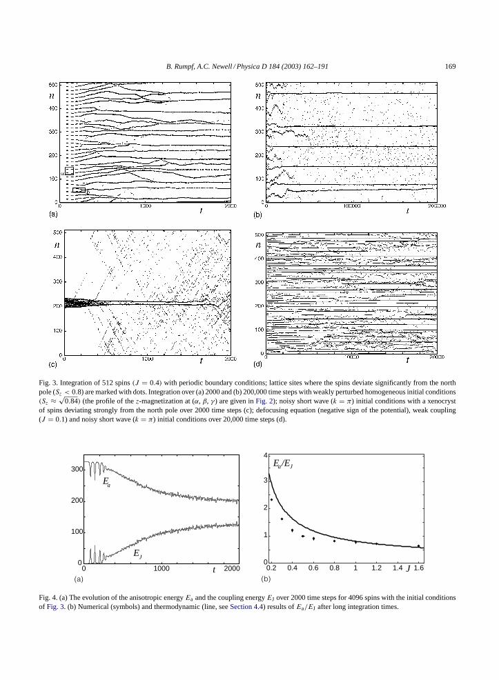
B. Rumpf, A.C. Newell / Physica D 184 (2003) 162–191 169
Fig. 3. Integration of 512 spins (J = 0.4) with periodic boundary conditions; lattice sites where the spins deviate significantly from the northpole (Sz < 0.8) are marked with dots. Integration over (a) 2000 and (b) 200,000 time steps with weakly perturbed homogeneous initial conditions(Sz ≈ √
0.84) (the profile of the z-magnetization at (α, β, γ) are given in Fig. 2); noisy short wave (k = π) initial conditions with a xenocrystof spins deviating strongly from the north pole over 2000 time steps (c); defocusing equation (negative sign of the potential), weak coupling(J = 0.1) and noisy short wave (k = π) initial conditions over 20,000 time steps (d).
J
E /Ea J
0
1
2
3
4
0.2 0.4 0.6 0.8 1 1.2 1.4 1.6
E
t
Ea
J0
100
200
300
0 1000 2000
(a) (b)
Fig. 4. (a) The evolution of the anisotropic energy Ea and the coupling energy EJ over 2000 time steps for 4096 spins with the initial conditionsof Fig. 3. (b) Numerical (symbols) and thermodynamic (line, see Section 4.4) results of Ea/EJ after long integration times.
170 B. Rumpf, A.C. Newell / Physica D 184 (2003) 162–191
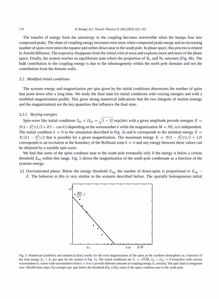
The transfer of energy from the anisotropy to the coupling becomes irreversible when the humps fuse intocompound peaks. The share of coupling energy increases even more when compound peaks merge and an increasingnumber of spins overcomes the equator and settles down near to the south pole. In phase space, this process is relatedto Arnold diffusion. The trajectory disappears from the initial critical torus and explores more and more of the phasespace. Finally, the system reaches an equilibrium state where the proportion ofHa andHJ saturates (Fig. 4b). Thebulk contribution to the coupling energy is due to the inhomogeneity within the north pole domains and not thecontribution from the domain walls.
3.2. Modified initial conditions
The systems energy and magnetization per spin given by the initial conditions determines the number of spinsthat point down after a long time. We study the final state for initial conditions with varying energies and with amodified magnetization profile. This gives strong numerical indications that the two integrals of motion (energyand the magnetization) are the key quantities that influence the final state.
3.2.1. Varying energies
Spin-wave like initial conditions Sxn + iSyn =√
1 − S2z exp(ikn) with a given amplitude provide energies E =
N(1−S2z )(1/2+J(1− cos k)) depending on the wavenumber k while the magnetization M = NSz is k-independent.
The initial condition k = 0 in the simulation described in Fig. 2a and b corresponds to the minimal energy E =N/2(1 − S2
z )/2 that is possible for a given magnetization. The maximum energy E = N(1 − S2z )(1/2 + 2J)
corresponds to an excitation at the boundary of the Brillouin zone k = π and any energy between these values canbe obtained by a suitable spin-wave.
We find that some of the spins condense near to the south pole eventually only if the energy is below a certainthreshold Eeq within this range. Fig. 5 shows the magnetization of the south pole condensate as a function of thesystems energy:
(i) Oversaturated phase: Below the energy threshold Eeq, the number of down-spins is proportional to Eeq −E. The behavior in this is very similar to the scenario described before. The spatially homogeneous initial
Σ|S |
E/N
S<0z
z
0
10
0.1 0.15
Fig. 5. Numerical (symbols) and analytical (line) results for the total magnetization of the spins in the southern hemisphere as a function ofthe total energy Ea + EJ per spin for the system of Fig. 1a. The initial conditions are Sz = √
0.84, Sxn + iSyn = 0.4 exp(ikn) with variouswavenumbers k; waves with wavenumbers from k = 0 to π provide different amounts of coupling energy EJ initially. The spin chain is integratedover 100,000 time steps. For energies per spin below the threshold (Eq. (18)), some of the spins condense near to the south pole.
B. Rumpf, A.C. Newell / Physica D 184 (2003) 162–191 171
condition in the above simulations just leads to the highest possible proportion of the south pole conden-sate.
(ii) Overheated phase: For high energies E > Eeq, no spins are flipped down so that this magnetization is zero.There is no south pole condensate beyond this threshold; all spins end up in small fluctuations near the northpole.
3.2.2. Modified magnetization profileWe have seen that only long-wavelength fluctuations create peaks. In contrast, high energetic initial conditions
with short-wavelengths melt away such peaks of spins deviating significantly from the north pole. This occurs foran initial condition of a small amplitude k = π spin-wave (corresponding to the maximum energy in Fig. 5) wherethe spins within a small domain are flipped to the southern hemisphere. Fig. 3c shows the destruction of such adomain in a bath of k = π waves. The system ends up in an irregular state where all spins are near to the north pole.
3.3. Modified equations of motion
The scenario we have described is widespread in dynamical systems and not a specific feature of the Landau–Lifshitzequation. A comparison of this scenario with self-focusing in related systems indicates that the main conditions forthe emergence of coherent structures are:
(i) the low-amplitude dynamics is governed by an NLS-type of equation,(ii) the system is nonintegrable,
(iii) there are two integrals of motion.
The first of these points basically characterizes the dynamics of nonlinear dispersive systems on long scales. Thefocusing DNLS is the system most closely related to the spin chain. Also the case of a defocusing nonlinearity will beconsidered. The importance of nonintegrability will be shown by the comparison to the integrable Ablowitz–Ladikdiscretization of the NLS equation. On the other side, we will study a system with broken rotational symmetry thatonly conserves the Hamiltonian.
3.3.1. Defocusing equationThe formation of coherent structures in discrete nonintegrable systems is not an exclusive property of ‘ focusing’
types of DNLS or Landau–Lifshitz equations. The Landau–Lifshitz equation Sn = Sn × (J(Sn−1 + Sn+1)− Snzez)
with a negative (‘easy-plane’ ) anisotropy corresponds to the defocusing DNLS equation. For weak coupling constants(J = 0.1), short-wavelength (k = π) initial conditions produce coherent structures with spins condensing in theequator region where the anisotropic energy has now its minimum. Fig. 3d shows this weak focusing process forthe spin chain.
3.3.2. DNLS equationThe focusing nonintegrable DNLS iφn = J(φn+1+φn−1−2φn)+2|φn|2φn has the properties (i)–(iii) just like the
Heisenberg spin chain. Fig. 6a shows the spatiotemporal pattern for the DNLS of lattice sites with high-amplitudesthat is very similar to the one described in Section 3.1 (Fig. 2a). Again, an unstable periodic pattern emerges froma phase instability of the homogeneous state that is unstable itself.
The first and the second phase instability are well-known as direct consequences of (i) and (ii). The second phaseinstability has been studied in detail in the context of NLS equations. In phase space, it is related to degenerate toriwith less than the maximum dimension. Such critical tori exist in integrable as well as in nonintegrable systems;they may be stable or unstable. The stability of these tori is related to double points in the spectral transform [10].

172 B. Rumpf, A.C. Newell / Physica D 184 (2003) 162–191
Fig. 6. Integration of the various versions of the DNLS equation (J = 0.4) with 512 lattice sites and periodic boundary conditions. The initialconditions are φn = 0.2 plus noise, lattice sites with |φ| > 0.25 are marked with dots. (a) Integration of the DNLS over 2000 time steps; (b)integration of the integrable version of the DNLS over 2000 time steps; (c) DNLS with a contribution −2φn and a symmetry breaking field0.2φ′
n over 10,000 time steps; (d) DNLS with a symmetry breaking contribution 0.02φ′n over 10,000 time steps.
The spectrum of the Lax-operators has been analyzed both for an integrable and a nonintegrable version of theDNLS equation.
The fusions of humps lead to peaks with high-amplitudes (Fig. 6a) and finally high-amplitude xenocrysts emergefrom a low-amplitude turbulent background. The whole process is very similar to the one of the Landau–Lifshitzequation (Fig. 3a). The correspondence persists even in a domain where the additional nonlinear terms in theLandau–Lifshitz equation are not small. The DNLS-peaks may have different heights while the spin-peaks arealways south pole states. The radiation of low-amplitude fluctuations during the merging of peaks is related tohomoclinic chaos following the breakup of Kolmogorov–Arnold–Moser tori. By discussing the Melnikov-functionof the critical tori [11] have detected homoclinic crossings in the nonintegrable NLS. The horseshoe of the homocliniccrossings creates the disorder following the fusion of two peaks.
A phenomenon similar to the merging of peaks was found in a continuous nonintegrable NLS equation [7]. Unlikesolitons in integrable systems, collisions of solitary solutions of nonintegrable equations lead to a transfer of powerfrom the weaker soliton to the stronger one while low-amplitude waves are radiated. The resulting two-componentsolution contains a decreasing number of growing solitons immersed in a sea of weakly turbulent waves. In con-tinuous systems, energy is drained by infinitesimal scales while the spatial discretization defines a minimal lengthscale.

B. Rumpf, A.C. Newell / Physica D 184 (2003) 162–191 173
3.3.3. Integrable DNLS equationHomoclinic chaos as a source of radiation is absent in integrable systems. The comparison with the integrable
DNLS iφn = J(φn+1 + φn−1 − 2φn) + |φn|2(φn−1 + φn+1) shows this implication of the nonintegrability (ii).The integrable NLS equation exhibits the primary phase instability, but not the fusing of neighboring peaks. Whilethe dynamics is similar to the nonintegrable system initially, the peaks do not merge (Fig. 6b). Consequently, nocoherent structures evolve and the system does not settle down in a disordered equilibrium state. The quasiperiodicappearance of humps with relatively low-amplitudes reflects the phase space structure of nested tori.
3.3.4. Particle nonconserving equation of motionWhile the irreversible focusing process is a consequence of nonintegrability, it also depends on the existence of
some remaining integrals of motion. The generation of coherent structures is very sensitive to perturbations thatdestroy one of the remaining integrals. The property (iii) may be changed by breaking the rotational symmetry withthe contribution εRe(φn) in the NLS equation. The equation is still of Hamiltonian type, but the modulus-squarenorm
∑ |φn|2 is not conserved. Additional contributions ∼ω∑ |φn|2 to the Hamiltonian and the corresponding
term ∼ωφ in the equation of motion iφn = J(φn+1 +φn−1 −2φn)+ωφn +εRe(φn)+2|φn|2φn are now relevant forthe dynamics (in the symmetric case, this term just describes the same dynamics in different rotating frame systems;in the symmetry broken system, the external field ε is stationary in the system that rotates with the frequency ω).Depending on the sign of ω, two different scenarios are observed:
ω < 0: The onset of self-focusing for small times is similar to the symmetric case. However, the peaks emergingfrom the fusing process disintegrate eventually into small amplitude fluctuations (Fig. 6c).
ω ≥ 0: The onset of the focusing process is again similar to the one with particle conservation, but after about5000 time steps growing amplitude fluctuations lead to a disordered state. Unlike the rotationally symmetricsystem, high particle densities are not confined to small islands in a sea of low particle density fluctuations.The nonconservation of the particle number leads to high (but finite) particle density fluctuations everywhere(Fig. 6d).
In the spin chain, similar effects can be reached with an external magnetic field that is perpendicular to theanisotropy axis ez and an additional z-field. The Hamiltonian now contains the additional Zeeman terms εSx +ωSz.Due to the broken rotational symmetry the total magnetization is no longer an integral of motion.
3.4. The leapfrog-discretization of the KdV equation
Iterations of the leapfrog-discretization of the KdV equation exhibit a scenario of merging peaks that is verysimilar to the one found in NLS or spin equations. However, the leapfrog system undergoes a rapid unboundedgrowth similar to the blow-up in two-dimensional NLS-systems. While the Heisenberg spin chain has a well-definedequilibrium, the leapfrog system allows us to study the conditions for blow-ups in constrained systems. We studythis phenomenon for two initial conditions, the k = 2π/3 mode with a strong correlation of u and v, and for whitenoise with no correlation of u and v. The system consists of 1020 lattice sites with periodic boundary conditions.
3.4.1. Correlated initial conditionsThe monochromatic wave with the wavenumber k = 2π/3 as initial condition yields an exact but phase-unstable
[18] solution of the leapfrog-iteration (3a) for a sufficiently small step-size. This mode is particularly relevant for astability analysis since it is the fastest growing mode for a step-size τ > 2/(3
√3). Setting u1(n) = v1(n) provides
the maximum correlation of u and v. The pattern of peaks Fig. 7a (lattice sites with high u(n)2 + v(n)2) emergesin a manner similar to the spin- and NLS-systems (Figs. 3 and 6):

174 B. Rumpf, A.C. Newell / Physica D 184 (2003) 162–191
n
m0
1000
33200 33600 34000 34400
n
m0
200
400
600
800
1000
0 1000 2000
(a) (b)
Fig. 7. Iteration of the leapfrog-discretized KdV (3) for a k = 2π/3 wave (a) and for white noise initial conditions (b) with periodic boundaryconditions. The amplitude of u(n) = v(n) is 0.1 initially in (a). Locations with high-amplitudes (the sum of u(n)2 over five subsequent steps isgreater than 0.1) are marked with a dot. (b) The threshold of
√u2 + v2 is 0.045 while the noise level ∼0.01.
(i) Regular behavior: The initial low-amplitude wave is below the threshold to be traced in Fig. 7 for m < 400.(ii) Merging humps: A phase instability of the initial k = 2π/3 wave leads to a modulational pattern with a
wavelength of about 20 lattice sites that reaches the threshold at m ≈ 400 so that a spatially periodic patternemerges for 400 < m < 600. These periodic humps are wave-packets of the initial short wave moving towardshigher n. Similar to the spin- and NLS-systems, this pattern itself is slowly modulated. The humps approacheach other and merge so that a decreasing number of peaks of increasing intensity survive. Solitary solutions thatare high and fast sweep away slower ones. The peaks speed and amplitude increase while the width decreasesduring this process. They accumulate high amounts of the conserved quantity 〈uv〉 just like the spin-downdomains gather magnetization. Fig. 8 shows the cumulated conserved quantity
∑nl=1 um(l)vm(l) as a function
of n (for n = N, it is conserved) at the beginning (m = 1) and at m = 2500 when the solitary waves havedeveloped. While the conserved correlation
∑u(n)v(n) is equally distributed in space initially, the formation
of solitary wave-packets gathers an increasing amount of the correlation in small xenochrysts immersed inuncorrelated low-amplitude fluctuations. Up to this point, the process is very similar to the self-focusingscenario presented in the spin- and NLS-systems.
n
u (l)v (l)
m=1
m=2500
l=1
n
m mΣ
0
1
2
3
4
5
0 200 400 600 800 1000
Fig. 8. Cumulated energy∑n
l=1 um(l)vm(l) for the simulation of Figs. 7 and 9 as a function of the lattice site n at the time steps m = 1 and 2500.

B. Rumpf, A.C. Newell / Physica D 184 (2003) 162–191 175
m
(u (n)+v (n))2n m mΣ
- (u (n)-v (n))2n m mΣ
-1
-0.5
0
0.5
1
33200 33600 34000 34400m
(u (n)+v (n))2n m mΣ
- (u (n)-v (n))2n m mΣ
-20
-10
0
10
20
30
40
0 1000 2000
(a) (b)
Fig. 9.∑
(u(n)+ v(n))2 and − ∑(u(n)− v(n))2 of the leapfrog-discretized KdV system as a function of time m for the k = 2π/3 wave (a) and
for the white noise initial condition (b).
(iii) Rapid divergence: However, despite the fact that for a long time the system appears to reach a statisticallystationary state, in the end it is clear that no equilibrium is attained and the local amplitude rapidly diverges.At m ≈ 2960, two peaks merge at n ≈ 420 creating an all-time high of the amplitude that apparentlyexceeds a certain threshold locally. This highest peak now starts to grow rapidly so that the iteration is derailedwithin a few time steps. The features of this rapidly growing ‘monster’ solution will be described in the nextsection.
Unlike the modulus-square norm of the continuous KdV equation,∑
u(n)2 is not conserved in the whole process.Fig. 9a shows
∑(u(n) + v(n))2 and − ∑
(u(n) − v(n))2 as a function of the time m.∑
(u(n) + v(n))2 equals4
∑u(n)v(n) initially while − ∑
(u(n)−v(n))2 starts at zero; the sum of both quantities ∼〈u(n)v(n)〉 is conserved.In the ‘ reversible’ range m < 400 (i), both quantities increase and recur to their initial value periodically. As themerging of peaks starts (ii), they settle to almost constant values undergoing only a very slow increase. This behaviorresembles Fig. 4 up to the final blow-up (iii) where both quantities diverge rapidly.
Initial condition with a low amount of 〈uv〉 lead to solitary solutions that do not reach the threshold for theblow-up. Their growth ends when a few of them have absorbed this conserved quantity and move with the samespeed. This state however is also unstable because of an instability to be described in the next section.
3.4.2. Uncorrelated white noise initial conditionsUncorrelated low-amplitude white noise initial conditions 〈uv〉 = 0 lead a creeping nonlinear process that
suddenly ends up in the same sort of local rapid divergence of the amplitude. The time elapsing until the systemblows up is inversely proportional to the square of the noise amplitude. For random white noise initial conditionswith the same amplitude it is Poisson-distributed.
Fig. 7b shows the spatiotemporal pattern of locations where the amplitude slightly exceeds the noise level. Unlikethe correlated case, there is no spatiotemporal pattern of merging peaks. A change in the amplitude profile of thenoise background is hardly detectable even shortly before the blow-up occurs. Again three phases of the dynamicalbehavior can be distinguished:
(i) Regular behavior: For about 32,000 time steps, the amplitudes are at the level of the noise imposed by theinitial conditions. During this time, physical structures such as solitons can be simulated reliably when theyare imposed by the initial conditions.

176 B. Rumpf, A.C. Newell / Physica D 184 (2003) 162–191
v (n)
n
m
m=33500
m=34000
m=34300-0.04
0
0.04
400 500 600 700
u (n)
n
34374
-1030
1030
0
530 540 550 560
u (n)
n
m
m=4100
m=4300
m=4500
-0.04
0
0.04
400 500 600 700
u (n)
n
m
m=33500
m=34000
m=34300
-0.04
0
0.04
400 500 600 700
(b)
(d)(c)
(a)
Fig. 10. Profile of the peak evolving out of white noise (Fig. 7b). Low-pass filtered amplitudes u(n) (a) and v(n) (b) at m = 33,500, 34,000 and34,300. (c) u(n) at m = 34,374 two time steps before the iteration breaks down. The dotted line is the analytical solution. (d) u(n) at m = 4100,4300 and 4500 for smooth initial conditions v0(n) = 0, u0(n) = 0.01/ cosh 2(n − 510) is very similar to the simulation (a).
(ii) Creeping focusing process: A weak nonmoving maximum emerges at m ≈ 33,500, n ≈ 550 and grows slowly.Fig. 10 shows the low-pass filtered amplitudes of u(n) (a) and v(n) (b) of this structure at m = 33,500, 34,000and 34,300. The low-pass filtered amplitude changes significantly with each time step, but very little with twosubsequent time steps. Fig. 11 shows the corresponding spectral density.
(iii) Rapid divergence: After a slow growing process over about 1000 time steps this structure suddenly starts togrow rapidly and derails the iteration. Fig. 10c shows u(n) for this solution at m = 34,374. Fig. 11 showsthe spectral density of 〈uv〉 at the time steps of Fig. 10. This solution (which we call the ‘monster’ solutionbecause its spatial structure resembles the Loch Ness monster with several undulations of its tail sticking outof the water) appears to be the systems canonical trajectory towards infinite amplitudes.
Monsters are strongly localized: left to the highest negative amplitude, the head of the monster, the amplitudesare close to zero. Right to the head, the amplitude of the zig-zag tail decreases rapidly. The monster moves to theleft by one lattice site with each time step. There are also monsters that move to the right; their shape is related toleft-moving monsters as u(n) → −u(−n). Most significantly, the amplitude of the monster is squared by every timestep so that the monster grows as exp(exp(m)). Fig. 7b shows a delta-shaped broadening zone of high-amplitudesnear the blow-up since the tail is growing while the head moves towards small n.

B. Rumpf, A.C. Newell / Physica D 184 (2003) 162–191 177
FT(<u(n)v(n+r)>)
k
m=4100
m=4300
m=4500
π/30
0
0.0005FT(<u(n)v(n+r)>)
k
m=33500
m=34000
m=34300
π/30
-0.001
0
0.001
(a) (b)
Fig. 11. Spectral density (defined as the Fourier-transform of the correlation 〈u(n)(v(n + r) + v(n − r)) + v(n)(u(n + r) + u(n − r))〉, r ≤ 100for the simulation of Fig. 7b at the time steps of Fig. 10. (a) Shows the slowly growing solution that leads to the monster. (b) The correlation forthe smooth initial conditions of the simulation (Fig. 10d).
This solution can be calculated analytically. For a state um(n) = Aa(n) with a high-amplitude A, the linearterms of Eq. (3) may be neglected. We assume that the structure grows quadratically and moves to the right asum+1(n) = 2τA2a(n − 1). Setting a(n) = 0 for n > 0 and for negative odd n, we get the solutions a(0) = 1,a(−2) = (1 −√
5)/2, a(−2n− 2) = (1 −√
1 + 4a(−2n)2)/2 as the solution of a(n− 1) = a(n− 1)2 −a(n+ 1)2.The right moving solution is obtained by setting a(n) → −a(−n). The dotted line in Fig. 10c shows this solutionwhere the monster’s head is submerged.
Most significantly, the conserved quantities 〈u〉, 〈v〉 and 〈uv〉 are zero for this solution; the monster needs noexternal food source for its growth. On the other side, it rapidly produces high amounts of 〈u2 + v2〉 (Fig. 9b).
A blow-up with these characteristic features follows from various initial conditions. In the previous section wehave described its evolution out of solitary solutions that emerge from a Benjamin–Feir type of instability and exceeda certain threshold after the merging process. It can also grow out of the noise between these solitary solutions orout of weak white noise through a much more dramatic type of instability.
4. Statistical analysis of the final state
In this section we will give a detailed interpretation of these results. The merging of peaks corresponds to anArnold diffusion process in phase space that transfers the trajectory from the initial critical torus to less distinctiveparts of the shell of constant energy 〈H〉 = E and magnetization 〈M〉 = M. The numerical findings indicatethat the characteristics of the final solution are determined by the values of the integrals of motion, i.e. that thesystem reaches a thermodynamic equilibrium. One can therefore establish thermodynamic connections betweenmacroscopic observables of the final solution and the integrals of motion. We will compute the equilibrium statisticsof the system and compare the results to our numerical findings.
4.1. The partition function
4.1.1. Low-temperature approximationThe numerical findings suggest that for low energies the spins point to small regions near to the poles (Fig. 1a)
and avoid the region nearer to the equator. With σn = ±1 one may approximate spins near to the north or south

178 B. Rumpf, A.C. Newell / Physica D 184 (2003) 162–191
pole as
Snz ≈ σn(1 − 12 (S
2nx + S2
ny)). (4)
Low-amplitude fluctuations near the north pole are represented by σn = 1 and small values of Snx/y. The coherentstructures with spins near to the south pole correspond to σn = −1. This matching height of all peaks is the maintechnical advantage of the spin chain. Assuming that σnσn+1 = 1 holds for almost all n (i.e. the number of domainwalls is small), one may approximate
∑σnσn+1S
2nx/y ≈ ∑
n S2nx/y. If all spins are close to the poles, the approximate
Hamiltonian
Heff =∑n
12 (S
2nx + S2
ny) + J(S2nx + S2
ny) − J(SnxSn+1x + SnySn+1y) − Jσnσn+1, (5)
represents a chain of coupled harmonic oscillators (Snx, Sny) and a chain of Ising spins σn. The approximationholds if the energy is low and the magnetization is close to the maximum, i.e.
∑(1 − Snz)/N 1. It neglects
the coupling between the oscillators Snx/y and the Ising spin σn so that the Hamiltonian splits up into a spin-waveHamiltonian Hw(Snx, Sny) and an Ising Hamiltonian HI(σn). Hw contains the lowest order terms of Snx/y andneglects anharmonic energy contributions of neighboring spins that point to the same hemisphere.HI accounts forthe coupling between up- and down-spins. In terms of the stereographic projection, Hw contains the terms thatprevail for |φ| 1 whileHI allows for the contributions for |φ| 1. The nonlinearity is only reflected in the Isingmagnet.
The magnetization as a second integral of motion may be approximated as
Meff =MI(σ) +Mw(Sx, Sy) =∑n
σn −∑n
1
2(S2
nx + S2ny), (6)
if most of the spins point to the north pole. Again this approximation neglects higher order terms in Snx/y andcontributions σnS
2nx/y with σn = −1.
4.1.2. Grandcanonical partition functionThe phase space surface on whichM andH are constant can be computed most easily using the grand partition
function
y(β, γ) =∫
e−β(Heff−γMeff ) dΓ (7)
with two parameters β and γ . Unlike the canonical ensemble [19], the grandcanonical ensemble reflects the secondintegral of motion by the parameter γ that controls the system’s magnetization. β is the inverse temperature whileγ is an equivalent of a magnetic field or chemical potential. The exponent in (7) is a sum Heff − γMeff =(Hw − γMw) + (HI − γMI) of a spin-wave contribution
Hw − γMw =∑n
J
2((Snx − Sn+1x)
2 + (Sn+1y − Sn+1y)2) + 1 + γ
2(S2
nx + S2ny), (8)
that depends only on Snx, Sny and an Ising contribution
HI − γMI = J∑n
(1 − σnσn+1) − γ∑
σn, (9)
that depends only on σn. The partition function (7) of the whole system is the product y = ywyI, where yw isobtained by an integration over the variables Snx, Sny, while yI is a sum of the configurations of the Ising spins σn.The grand partition function of the N Ising spins
yI = ( cosh (γβ) + µ)N (10)
B. Rumpf, A.C. Newell / Physica D 184 (2003) 162–191 179
with the abbreviation µ =√
sinh 2(γβ) + e−4Jβ is just the canonical partition function of an Ising magnet in anexternal field γ . The linear dynamics of Snx and Sny has the symplectic structure Snx/y = ±∂Hw/∂Sny/x so that aphase space volume element may be approximated as dΓ = ∏
dSxn dSyn. For β 1, the grand partition functionof the spin-waves can be obtained by integrating of dΓ = ∏
dSxn dSyn from minus to plus infinity. Using theabbreviation A = √
J/2 + (1 + γ)/8 + √(1 + γ)/8 the Gaussian integrals yield
yw(β, γ) =(
π
A2β
)N
. (11)
4.2. Thermodynamic relations
4.2.1. Energy and magnetizationThe thermodynamic properties of the equilibrium state may be derived from the grand partition function ln y(β, γ) =
ln yw + ln yI. The parameters β, γ and the conserved quantities 〈H〉 = E, 〈M〉 = M are connected by
M = Mw + MI = 1
β
∂
∂γ( ln(yw) + ln(yI)) = N
(− 1
βλ+ sinh (γβ)
µ
), (12)
E = Ew + EI =(
γ
β
∂
∂γ− ∂
∂β
)( ln(yw) + ln(yI)) = N
β
(1 − γ
λ
)+ 2NJ e−4Jβ
cosh (γβ)µ + µ2(13)
with λ =√
4J(1 + γ) + (1 + γ)2. The partition function is valid for small energies per lattice site E/N 1 and forsmall mean deviations 1−M/N 1 of the spins from the north pole. Low-amplitude initial conditions without hugedeviations from the north pole correspond to magnetizations in the interval 1−E/N ≤ M/N ≤ 1−E/(N(1+4J)).The lower bound corresponds to a spatially homogeneous initial condition while a wave with k = π defines theupper bound.
MI, EI, Mw, Ew are the physically most interesting quantities:
MI is the magnetization of the Ising system and measures the total extent of the coherent structures. At itsmaximum MI = N, all spins point up while smaller values N > MI > M indicate the existence of coherentstructures where the spins point down.
EI is the positive coupling energy of the domain boundaries and determines the number of coherent structures.Mw is the negative magnetization of small fluctuations.Ew is the positive energy of small fluctuations and comprises a coupling term and an anisotropic term.
These quantities can be found by computing β and γ as functions of E and M and then plugging β and γ in theexpressions for EI, MI, Ew, Mw. (12) and (13) can be solved analytically for the low-energy case E/N 1. Thesolution (Fig. 12) is qualitatively different in the ‘oversaturated phase’ with M < Meq and in the ‘overheated phase’Meq < M < Mπ with Meq = N − E/
√1 + 4J .
4.2.2. Oversaturated phase M < Meq
(i) The temperature β−1 ≈ E/N 1 is almost independent of M.(ii) The chemical potential γ ≈ E e−2JN/E/
√2N(Meq − M) ≈ 0 is exponentially small unless the magnetization
comes very close to the transition point where this approximation breaks down.(iii) Almost the total energy Ew ≈ E is absorbed by the fluctuations while the surface energy EI ∼ e−2JN/E ≈ 0
is exponentially small.

180 B. Rumpf, A.C. Newell / Physica D 184 (2003) 162–191
0.05
0.1 -0.05 -0.01
-3
0
3 γ
M
Ew
w
βγ
γ
β
M MMM
M
s
eq0
w
π
-1
-1
-3
-2
-1
0
1
2
3
-0.1 -0.09 -0.08 -0.07 -0.06 -0.05 -0.04
0.05
0.1 -0.05 -0.01
-0.3
0
0.3-1β
M
Ew
w
(c)
(a) (b)
Fig. 12. The temperature β−1(Mw, Ew) (a) and the chemical potential γ(Mw, Ew) (b) as obtained from the Eqs. (12) and (13). The energy isfixed as Ew = 0.1 in (c)
(iv) The fluctuations share Mw ≈ −E/√
1 + 4JN of the magnetization is independent of the total magnetization.The remainder of M −N is absorbed by the spins that are flipped down. The share of spins that is flipped downis at most of the order of the energy.
4.2.3. Overheated phase Meq < M < Mπ
(i) The temperature
β−1 = (E + M − N)(4J(M − N) + E + (M − N))
(4J(M − N) + 2(E + (M − N)))N. (14)
(ii) The chemical potential
γ = (E + M − N)2
4J(M − N)2 + 2(E + M − N)(M − N)− 1, (15)
both have a singularity at Ms = N − E/(2J + 1). The temperature is positive between Mw = M0 and thesingularity because the number of accessible states grows with the energy in this range. Beyond the singularity,more energy leads to a decreasing number of states so that the temperature is negative.
(iii) The spin-waves Ew ≈ E again absorb the bulk of the energy while EI ∼ e−2JN/E ≈ 0.(iv) The Ising-magnetization is near to its maximum MI ≈ N independently of M. Fluctuations contribute the
magnetization Mw ≈ −E/λ.

B. Rumpf, A.C. Newell / Physica D 184 (2003) 162–191 181
4.2.4. Transition at Meq
The solution for MI explains the transition behavior of Fig. 5 (Section 3.2.1) and the emergence of coherentstructures quantitatively. While the oversaturated phase corresponds to long spin-wave initial conditions, the ther-modynamic equilibrium state is characterized by coherent structures, i.e. spins pointing to the south pole. Belowthe threshold Meq, the Ising-magnetization MI deviates significantly from its maximum MI = N and the number ofspins that point down increases linearly with Meq − M. Above the transition the Ising-magnetization deviates verylittle from its maximum MI = N, so there are no coherent structures.
In both phases almost all energy is absorbed by low-amplitude fluctuations. The surface energy EI is exponentiallysmall, so that the spins form a very small number of domains. The higher number of domains obtained numericallyindicates that the system does not thermalize completely on reasonable time scales.
As the spins interact only pairwise with a short range in one dimension, the transition between the two phases isof diffuse type and not a genuine phase transition. γ and MI are analytic functions. The slope of γ increases rapidlywithin a small interval ∼e−4JN/E at Meq so that the transition approaches a phase transition as the energy goes tozero.
4.3. The entropy
4.3.1. The shape of the entropy functionThe thermodynamic reasons for coherent structures are best described in terms of the systems entropy. The
conserved quantities M and E are known from the initial conditions rather than the arguments β, γ of the grandpartition function. Consequently, the entropy as a function of M and E is the appropriate thermodynamic potential.The entropy follows from the grand partition function by two Legendre transformations
S = ln(y) + β(E − γM) =(
1 − β∂
∂β
)ln(y). (16)
Both the spin-waves and the Ising system contribute to the entropy. The two systems can get different shares EI,MI and Ew, Mw of the two conserved quantities E and M. The entropy of the Ising has the form ∼−EI ln(EI/N).The spin-wave entropy per lattice site is given by Sw/N = ln Ω, where the total number of accessible microstatesis ΩN with
Ω = (Ew + (1 + 4J)Mw)(Ew + Mw)
NMw. (17)
So the entropy of small fluctuations depends on the energy as ∼N ln(Ew/N). Both systems are coupled thermally, sothey have matching temperatures β−1. Using β = ∂S/∂E we reestablish the fact that the Ising energy EI/N ∼ e−2Jβ
is exponentially small compared to the energy of the fluctuations Ew/N ∼ β−1 for low energies. The resulting Isingentropy is again exponentially small SI ∼ e−2Jβ compared to the spin-waves contribution Sw ∼ − ln β + const.
Consequently, the main part of the entropy arises from the degrees of freedom of waves with small amplitudeswhile the Ising system only provides an almost constant contribution. The Ising system can absorb some of thesystems magnetization without changing its energy and entropy significantly. By doing that, the fluctuations share ofmagnetization can also change allowing the fluctuations to maximize their entropy. The maximum of Sw = N ln Ω
as a function of Ew and Mw is approximately the total entropy maximum.Fig. 13a shows the number of states per lattice site Ω of the fluctuations as a function of Mw and Ew. It has the
shape of a crest ascending towards higher energies. All possible small amplitude states corresponding to positiveΩ are in a triangular region limited by two highly ordered solutions (M0 = −Ew and Mπ = −Ew/(4J + 1)) andby the systems total energy Ew = E.

182 B. Rumpf, A.C. Newell / Physica D 184 (2003) 162–191
J=0.4J=0.1
M
M MEM
eq 0w
wπ
Ω
-0.16
-0.04
-0.08
-0.04
0
0.01
0.02
M
MM
M
M
E0
eqs
w
w
π
Ω
-0.1-0.08
-0.04
0.05
0.1
0
0.01
0.02
0.03
(a) (b)
Fig. 13. Ω for the spin chain as a function of Ew and Mw: (a) Focusing equation with J = 0.4. The focussing process corresponds to the arrow onthe left slope, the arrow on the crest sketches the merging of peaks. The arrow on the right slope represents the destruction of coherent structuresby short-wavelength fluctuations. (b) Defocusing case for J = 0.1 and 0.4. The line Mπ crosses Ew = 0 for 4J − 1 = 0.
The area between the lines M0 and Meq again represents the oversaturated phase. The rim M0 = −Ew with Ω = 0corresponds to a monochromatic wave with k = 0. Long-wavelength solutions (which are also representative forcontinuous systems) are located at the slope near to this line. Such fluctuations have a low ratio E/(N−M). Solutionsthat include high peaks may have even smaller values M < N+M0. However, their inert down-magnetized domainshave little influence on the thermodynamics and these states are similar to the ones at M0.
The overheated phase is located between the lines Meq and Mπ. The rim Mπ = −Ew/(4J + 1) with Ω = 0represents a wave k = π at the boundary of the Brillouin zone. This wave has the highest ratio E/(N − M) of allsolutions.
The systems total energy Ew = E gives a third boundary of the accessible states. The absolute maximum of theentropy is located on this boundary at Mw = −E/
√4J + 1.
4.3.2. Coherent structuresThe formation of peaks (i.e. down-magnetized domains) can be understood as the maximization of the entropy
under the restriction of the conserved quantities. Formation and merging or destruction of coherent structures isrepresented by paths from the slopes to the crest and to the entropy maximum typifying the phenomena that havebeen observed numerically. While these are nonequilibrium processes since Mw and Ew are changing, Eq. (17)gives the equilibrium entropy for a system thermalizing at particular constant values of Mw, Ew:
(i) Formation of coherent structures in the oversaturated phase: For M < N+Meq (or Mw < Meq, e.g. for spatiallyhomogeneous initial conditions or long waves), the system can increaseMw < 0 and decreaseMI > 0 by flippingspins from the north to the south. In the entropy profile this means that the system is allowed to move from theM0-side in the direction towards Meq (along the arrow at the left slope in Fig. 13a). This leads to an increaseof the spin-wave entropy Sw for initial condition on the M0-side of the slope. This process stops when the crestis reached so that the ideal amount of magnetization Meq is allocated to the spin-waves. For long-wavelengthinitial conditions, the formation of coherent structures allows the exploitation of short-wavelength degrees offreedom to increase the entropy.
An additional increase of the fluctuations entropy may be reached by transferring energy from EI to Ew.This happens when merging down-magnetized domains reduce the domain wall energy contributing to EI. InFig. 3a we can identify the route along the crest Meq with this process. Finally, Ew absorbs almost all energyat the summit leaving little energy EI Ew for domain boundaries. The resulting magnetization of the Ising

B. Rumpf, A.C. Newell / Physica D 184 (2003) 162–191 183
magnet is
MI = M + E√4J + 1
. (18)
(ii) Destruction of coherent structures in the overheated phase: For M > N + Meq (or 0 > Mw > Meq, e.g.a k = π-spin-wave as initial condition), flipping spins down is impossible because this would decrease theentropy. The opposite movement starting from the Mπ slope towards the crest Meq is only possible if somespins are already flipped down so that they may be flipped up now. This type of thermalization process occursfor initial conditions of spin-down xenochrysts immersed in short-wavelength low-amplitude fluctuations. Thisprocess ends if either all spins point up (MI = N) or if the ideal amount of magnetization Meq is allocated tothe spin-waves. The crest of the entropy may be approached from the Mπ-side by melting existing coherentstructures away (arrow at the right slope in Fig. 13c).
Fig. 5 compares the numerical and analytical results for the number of down-spins as a function of the total energy,while the total magnetization is fixed. For low energies (long wave initial conditions), a relatively big number ofspins points down so that MI is smaller. For higher energies (smaller wavelengths), the number of down-spinsdecreases and reaches zero at the transition point. In Fig. 13a, these initial conditions correspond to energies on aline M = const connecting points on the lines M0 and Mπ. The threshold of Fig. 5 corresponds to the intersectionpoint of the line M = const and the crest Meq(E). This threshold is obtained for any path that crosses Meq. Belowthe threshold, the spin-wave entropy can be maximized by flipping spins down according to Eq. (18)). Above thethreshold only an exponentially small share of spins point down. Again, the transition is analytic but very sharp.
We conclude that the thermalization of energy under the constraint of the second integral of motion produceshigh-amplitude peaks emerging from an irregular low-amplitude background. The formation of coherent struc-tures allows the system to increase its entropy of low-amplitude fluctuations by allocating the right amount ofmagnetization to the spin-waves. While the total magnetization M = Mw + MI is constant, the spin-wave partMw = − ∑
(S2xn + S2
yn)/2 can turn over magnetization to the Ising part MI = ∑σn that can attain any value in
the interval M ≤ MI ≤ N. This enhances the entropy of the spin-waves while the Ising entropy is negligible.The entropy increases with Ew so that almost all energy is allocated to the fluctuations. This explains the mergingprocess of the peaks where energy is transferred from EI to Ew.
4.4. Power spectrum and particle conservation
Spin-waves with a wavenumber k contribute the power
〈nk〉 = 1
β(2J(1 − cos k) + 1 + γ), (19)
to the Hamiltonian E = ∑k nkωk with nk = SkxS−kx +SkyS−ky and ωk = 2J(1− cos k)+1. The ‘particle number’∑
nk is related to the magnetization Mw. Fig. 14a compares the Rayleigh–Jeans distribution 〈nk〉 = T/(γ + ωk) tonumerical simulations:
(i) In the overheated phase below the transition, the distribution is independent of M since γ is exponentially small.The energy nkωk is distributed equally over the k-space while small wavenumbers have the highest power nk.The power spectrum Fig. 14a is almost unchanged throughout the oversaturated phase and the fluctuationsenergy per particle is constantly
√4J + 1. The systems surplus of particles condenses at the south pole state
with low energies per particle, i.e. some spins are flipped to the south pole. The Rayleigh–Jeans distributionis attained during the merging process starting from the peak-like spectrum of the initial monochromatic

184 B. Rumpf, A.C. Newell / Physica D 184 (2003) 162–191
π 2π0
nk
π 2π0
nk
(a) (b)
Fig. 14. Spatial power spectra of the spin chain averaged over 100,000 time steps after a previous integration over 100,000 time steps and thecorresponding Rayleigh–Jeans distributions (19). (a) Was obtained for homogeneous initial conditions, (b) follows from a noisy short wave(k ≈ 2π/3) initial condition related to negative β and γ .
wave. The fluctuations determine the equilibrium ratio of anisotropic energy and coupling energy (Fig. 4a) asEa/EJ = (
√4J + 1 − 1)−1. Fig. 4b compares this formula to the results of simulations with various coupling
parameters J . Deviations are due to the fact that the system does not reach the perfect equilibrium after theintegration. Some additional domain walls lead to slightly increased values of EI.
(ii) Above the threshold, γ strongly depends on M and E and the power spectrum is deformed. The temperaturebecomes negative in the strongly ‘overheated’ domain since the entropy as a function of E decreases forM > M∞. In this range, most of the energy is due to short waves (see Fig. 14b) with β−1 ≈ −0.2, γ ≈ −2.7).
4.5. Defocusing equation
Thermodynamics of the ‘defocusing’ case (Fig. 3d) with a negative anisotropyH = ∑n J(1 − SnSn+1) − (1 −
S2zn)/2 is slightly more complex. We obtain Ω = (E + (4J − 1)Mw)(E − Mw)/Mw, where E is negative. We
distinguish two cases:
(i) For weak coupling 4J − 1 < 0, Ω has got a maximum at Meq = E/√−4J + 1 (see Ω-shell for J = 0.1 in
Fig. 13b). Ω is zero for M0 ≡ E < 0 and for Mπ ≡ −E/(4J − 1) < 0. Differently from the system witha positive sign of the nonlinearity in (1), now Mπ < M0, i.e. short-wavelength spin-waves have the lowestmagnetization for a given energy. Starting from Mπ, the system can approach Meq and increase its entropy byflipping down single spins. In contrast to the process described earlier, it is now favorable to store a maximumof energy in the domain boundaries.
(ii) For strong coupling (4J − 1 > 0), Ω as a function of M decreases in the whole interval of accessible values ofMw < M0 or Mw < Mπ and is zero at the homogeneous state Mw = M0 ≡ E and for short waves Mw = Mπ
(see J = 0.4 in Fig. 13b). The entropy of the spin-waves cannot be increased by decreasing the magnetization.Thermodynamics allows a weak focusing process by storing energy in domain walls starting from Mπ, but wehave found this process numerically only in the DNLS system.
4.6. NLS-systems versus spin systems
Thermodynamics supports the equivalence of spins and NLS-systems with respect to the formation of coherentstructures. Fig. 15 shows the nonlinear energy −|φn|4 at lattice sites n as a function of the particle number |φn|2 andthe corresponding anisotropic spin-energy (1−S2
nz)/2 as a function of the conserved negative magnetization 1−Snz;the points indicate typical states of the oscillators in equilibrium. The spin system has two states with a low-energyper lattice site. The north pole state is characterized by high energies per particle E/(N − M) while the specific
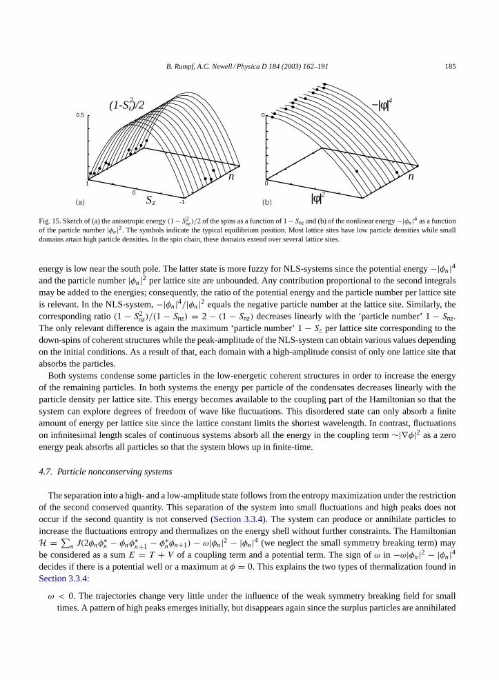
B. Rumpf, A.C. Newell / Physica D 184 (2003) 162–191 185
−|φ|
|φ|
n
4
2
0
0
(1-S )/2
S
n
z2
z
1
0
-1
0.5
(a) (b)
Fig. 15. Sketch of (a) the anisotropic energy (1 −S2nz)/2 of the spins as a function of 1 −Snz and (b) of the nonlinear energy −|φn|4 as a function
of the particle number |φn|2. The symbols indicate the typical equilibrium position. Most lattice sites have low particle densities while smalldomains attain high particle densities. In the spin chain, these domains extend over several lattice sites.
energy is low near the south pole. The latter state is more fuzzy for NLS-systems since the potential energy −|φn|4and the particle number |φn|2 per lattice site are unbounded. Any contribution proportional to the second integralsmay be added to the energies; consequently, the ratio of the potential energy and the particle number per lattice siteis relevant. In the NLS-system, −|φn|4/|φn|2 equals the negative particle number at the lattice site. Similarly, thecorresponding ratio (1 − S2
nz)/(1 − Snz) = 2 − (1 − Snz) decreases linearly with the ‘particle number’ 1 − Snz.The only relevant difference is again the maximum ‘particle number’ 1 − Sz per lattice site corresponding to thedown-spins of coherent structures while the peak-amplitude of the NLS-system can obtain various values dependingon the initial conditions. As a result of that, each domain with a high-amplitude consist of only one lattice site thatabsorbs the particles.
Both systems condense some particles in the low-energetic coherent structures in order to increase the energyof the remaining particles. In both systems the energy per particle of the condensates decreases linearly with theparticle density per lattice site. This energy becomes available to the coupling part of the Hamiltonian so that thesystem can explore degrees of freedom of wave like fluctuations. This disordered state can only absorb a finiteamount of energy per lattice site since the lattice constant limits the shortest wavelength. In contrast, fluctuationson infinitesimal length scales of continuous systems absorb all the energy in the coupling term ∼|∇φ|2 as a zeroenergy peak absorbs all particles so that the system blows up in finite-time.
4.7. Particle nonconserving systems
The separation into a high- and a low-amplitude state follows from the entropy maximization under the restrictionof the second conserved quantity. This separation of the system into small fluctuations and high peaks does notoccur if the second quantity is not conserved (Section 3.3.4). The system can produce or annihilate particles toincrease the fluctuations entropy and thermalizes on the energy shell without further constraints. The HamiltonianH = ∑
n J(2φnφ∗n − φnφ
∗n+1 − φ∗
nφn+1) − ω|φn|2 − |φn|4 (we neglect the small symmetry breaking term) maybe considered as a sum E = T + V of a coupling term and a potential term. The sign of ω in −ω|φn|2 − |φn|4decides if there is a potential well or a maximum at φ = 0. This explains the two types of thermalization found inSection 3.3.4:
ω < 0. The trajectories change very little under the influence of the weak symmetry breaking field for smalltimes. A pattern of high peaks emerges initially, but disappears again since the surplus particles are annihilated

186 B. Rumpf, A.C. Newell / Physica D 184 (2003) 162–191
(Fig. 6c). The system finally settles into a state of small fluctuations trapped in the potential well. However,some oscillators may escape from the local energy minimum and attain high-amplitudes for weaker symmetrybreaking fields.
ω ≥ 0. The system thermalizes in a state of high-amplitude fluctuations. In the DNLS-system, the amplitudescontinue to grow without bound since particles are created (Fig. 6d). Energy is transferred from the potentialto the coupling term so that T and |V | both grow. This growth stops finally so that the amplitudes remain finite.
It is the shape of the potential that leads to low-amplitude fluctuations by particle annihilation (i) or to particlecreation allowing high-amplitude fluctuations (ii) by thermalization. Interestingly, particle nonconservation doesnot led to fluctuations with infinite amplitudes in (ii); the particle production stops finally. The reason for this is themismatch of the orders of the potential energy V ∼ −|φ|4 and the coupling term that grows only quadratically withthe amplitude. Beyond certain high-amplitudes the coupling energy cannot absorb any more energy that is releasedby the potential. A further increase of the amplitude would distort the Rayleigh–Jeans distribution towards highwavenumbers and reduce the systems entropy; particle production has to stop therefore. In other words, the energyshell does not contain states with infinite amplitudes.
The Landau–Lifshitz equation with ω ≤ 0 leads to small fluctuations since the anisotropic energy has quadraticminima at the poles. The potential energy is maximal at the north pole for sufficiently strong values ω > 0, so thatlarge but finite fluctuations emerge.
4.8. Leapfrog-discretized KdV equation
The intermediate dynamics of the discretized KdV equation resembles the spin systems formation of an equilib-rium state. The blow-up however is an intrinsic nonequilibrium process. We study the phase space volume that isaccessible to the system during this process.
4.8.1. Phase space shellThe leapfrog-discretized KdV (3) is a nonlinear, area preserving mapping in the N variables u(n), v(n). The area
preserving property can be seen from the Jacobian
J =∣∣∣∣∣∣
(∂G(u(n), . . . )
∂u(l)
)I
I 0
∣∣∣∣∣∣ = 1, (20)
where I is the identity matrix and 0 is the zero matrix. G comprises the linear and the nonlinear derivative termof (3). The phase space that is accessible to the system is restricted by the integrals of motion
∑um(n)vm(n),∑
u2m(n) = ∑v2m+1(n) and
∑u2m+1(n) = ∑
v2m(n). Introducing the variables Pm(n) = um(n) + vm(n) andQm(n) = um(n) − vm(n), the conserved quantity
∑u(n)v(n) of (3) may be written as
2〈uv〉 = 2∑
u(n)v(n)/N = 1
2N
∑n
P(n)2 − 1
2N
∑n
Q(n)2, (21)
as the difference of two unbounded positive terms while the nonconserved modulus-square norm is
〈u2 + v2〉 =∑
(u(n)2 + v(n)2)/N = 1
2N
∑n
P(n)2 + 1
2N
∑n
Q(n)2. (22)
Solutions of (3) which correspond to physical solutions have u(n) ≈ v(n) so that Q(n) ≈ 0. Roughly speaking,P(n) is associated to the physical modes which are solutions of the original partial differential equation while Q(n)
is associated to spurious computational modes. The integrals 〈P〉 = ∑P(n)/N and 〈Q〉 = ∑
Q(n)/N are linked
B. Rumpf, A.C. Newell / Physica D 184 (2003) 162–191 187
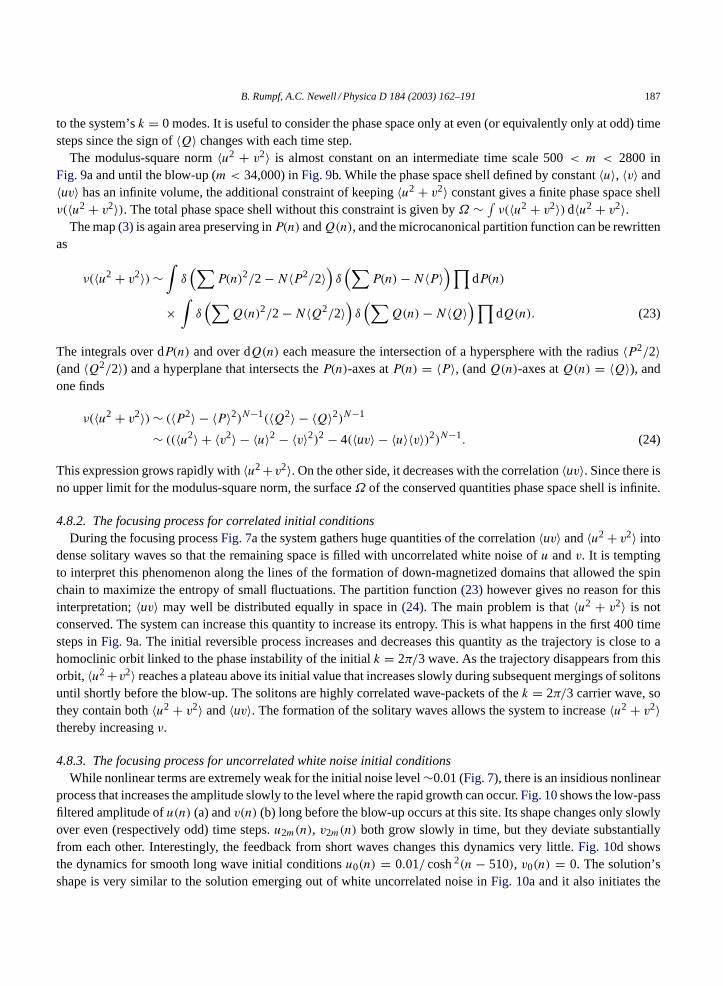
to the system’s k = 0 modes. It is useful to consider the phase space only at even (or equivalently only at odd) timesteps since the sign of 〈Q〉 changes with each time step.
The modulus-square norm 〈u2 + v2〉 is almost constant on an intermediate time scale 500 < m < 2800 inFig. 9a and until the blow-up (m < 34,000) in Fig. 9b. While the phase space shell defined by constant 〈u〉, 〈v〉 and〈uv〉 has an infinite volume, the additional constraint of keeping 〈u2 + v2〉 constant gives a finite phase space shellν(〈u2 + v2〉). The total phase space shell without this constraint is given by Ω ∼ ∫
ν(〈u2 + v2〉) d〈u2 + v2〉.The map (3) is again area preserving in P(n) and Q(n), and the microcanonical partition function can be rewritten
as
ν(〈u2 + v2〉) ∼∫
δ(∑
P(n)2/2 − N〈P2/2〉)δ(∑
P(n) − N〈P〉) ∏
dP(n)
×∫
δ(∑
Q(n)2/2 − N〈Q2/2〉)δ(∑
Q(n) − N〈Q〉) ∏
dQ(n). (23)
The integrals over dP(n) and over dQ(n) each measure the intersection of a hypersphere with the radius 〈P2/2〉(and 〈Q2/2〉) and a hyperplane that intersects the P(n)-axes at P(n) = 〈P〉, (and Q(n)-axes at Q(n) = 〈Q〉), andone finds
ν(〈u2 + v2〉) ∼ (〈P2〉 − 〈P〉2)N−1(〈Q2〉 − 〈Q〉2)N−1
∼ ((〈u2〉 + 〈v2〉 − 〈u〉2 − 〈v〉2)2 − 4(〈uv〉 − 〈u〉〈v〉)2)N−1. (24)
This expression grows rapidly with 〈u2 +v2〉. On the other side, it decreases with the correlation 〈uv〉. Since there isno upper limit for the modulus-square norm, the surface Ω of the conserved quantities phase space shell is infinite.
4.8.2. The focusing process for correlated initial conditionsDuring the focusing process Fig. 7a the system gathers huge quantities of the correlation 〈uv〉 and 〈u2 + v2〉 into
dense solitary waves so that the remaining space is filled with uncorrelated white noise of u and v. It is temptingto interpret this phenomenon along the lines of the formation of down-magnetized domains that allowed the spinchain to maximize the entropy of small fluctuations. The partition function (23) however gives no reason for thisinterpretation; 〈uv〉 may well be distributed equally in space in (24). The main problem is that 〈u2 + v2〉 is notconserved. The system can increase this quantity to increase its entropy. This is what happens in the first 400 timesteps in Fig. 9a. The initial reversible process increases and decreases this quantity as the trajectory is close to ahomoclinic orbit linked to the phase instability of the initial k = 2π/3 wave. As the trajectory disappears from thisorbit, 〈u2 +v2〉 reaches a plateau above its initial value that increases slowly during subsequent mergings of solitonsuntil shortly before the blow-up. The solitons are highly correlated wave-packets of the k = 2π/3 carrier wave, sothey contain both 〈u2 + v2〉 and 〈uv〉. The formation of the solitary waves allows the system to increase 〈u2 + v2〉thereby increasing ν.
4.8.3. The focusing process for uncorrelated white noise initial conditionsWhile nonlinear terms are extremely weak for the initial noise level ∼0.01 (Fig. 7), there is an insidious nonlinear
process that increases the amplitude slowly to the level where the rapid growth can occur. Fig. 10 shows the low-passfiltered amplitude of u(n) (a) and v(n) (b) long before the blow-up occurs at this site. Its shape changes only slowlyover even (respectively odd) time steps. u2m(n), v2m(n) both grow slowly in time, but they deviate substantiallyfrom each other. Interestingly, the feedback from short waves changes this dynamics very little. Fig. 10d showsthe dynamics for smooth long wave initial conditions u0(n) = 0.01/ cosh 2(n − 510), v0(n) = 0. The solution’sshape is very similar to the solution emerging out of white uncorrelated noise in Fig. 10a and it also initiates the

188 B. Rumpf, A.C. Newell / Physica D 184 (2003) 162–191
‘monster’ solution. The amplitudes may be described by continuous functions in space and time as u2m(n) = r(t, x)
and v2m(n) = s(t, x). Their dynamics is given by two coupled continuous KdV equations
r = sxxx − 6ssx, s = rxxx − 6rrx. (25)
These equations describe the long wave dynamics of the leapfrog system where the strength of the physical andthe computational mode is of the same order. Unlike the KdV equation, spatially homogeneous solutions of thecoupled KdV equations can be phase-unstable. Constant solutions r = r0 and s = s0 have the eigenvalues λ2 =−r0s0k
2 − (r0 + s0)k4 − k6. They are unstable for r0s0 < 0 and for r0 = 0, s0 < 0 (or for r0 < 0, s0 = 0). The
first instability is very similar to the Benjamin–Feir modulational instability and leads to traveling solitary waveswhich eventually can grow sufficiently large to access the ‘monster’ solution. The second is new and particularlyinteresting as it can initiate the ‘monster’ solution in a region where 〈uv〉 is zero. Its unstable mode has a shorterwavelength than the Benjamin–Feir mode (although still long compared to the lattice constant) and moreover growsfaster. We argue below that this saddle point in the phase space is accessed readily by an evolving solution becauseof an inverse flux of the power spectrum of the u, v correlation towards low wavenumbers. Once the system comesclose enough to this starting point, a localized solution grows irreversibly until it reaches the size necessary for therapidly growing monster solution which is a heteroclinic connection to infinity [20].
4.8.4. The blow-up of amplitudesAs (3) is nonintegrable, it is hardly surprising that the trajectory eventually separates from any orbit shadow-
ing a solution of the original partial differential equation. The trajectory simply can disappear from the originalKolmogorov–Arnold–Moser torus by Arnold diffusion and explore regions of the phase space that are most likelyconnected with high-amplitudes. The amazing finding is that this process can lead to such a rapid and unpredictabledivergence of the amplitude. This feature is absent in the spin system where the phase space itself is compact. InDNLS-systems, the coupling energy is restricted by the lattice constant and the conserved particle number
∑ |φ|2.The first restriction is absent in the two-dimensional continuous NLS equation, a canonical example of a systemwith wave collapses. The fixed energy is the difference of two energies
∫ |∇φ|2dV and∫ |φ|4dV that each are
not conserved and that can attain any value in a half-open interval. The corresponding conserved quantity in theleapfrog scheme is 2
∑u(n)v(n) = 1/2
∑n P(n)2 −1/2
∑n Q(n)2, where
∑P(n)2 and
∑Q(n)2 each may grow
indefinitely. This suggests that a blow-up occurs in systems where
(i) the phase space noncompact,(ii) the integral of motion constraining the phase space is the difference of two positive unbounded quantities.
We conjecture that the blow-up is the generic way of thermalization in such systems. The exploration of thephase space shell defined by a constant difference of two positive definite energies leads to finite-time singularitiessince both energies can grow unrestrictedly at the same rate. This may happen if a solitary structure grows beyonda certain threshold, or more surprisingly in a sudden eruption out of low-amplitude fluctuations. The analyticallyknown monster solution serves as the canonical highway to infinity during the blow-up.
Analogous to the collapse in the two-dimensional nonlinear Schrödinger equation this might be an inevitableconsequence of a condensation process. In that context, the spectral energy whose density is approximately ωknk
(where ωk = k2 is the frequency or energy of a wave vector k and nk is the particle density or waveaction) has anet flux to high wavenumbers. Because both
∑ωknk and nk are approximately conserved, this means that there
must be a corresponding flux of particles towards low wavenumbers. This flux leads to the growth of a condensateas particles are absorbed at k = 0. For the focusing NLS equation, this condensate is unstable and leads to theformation of collapsing filaments. But the instability is very robust and in fact the collapses begin before nk is allconcentrated at k = 0. As soon as there is sufficient nk near k = 0, the collapses begin.
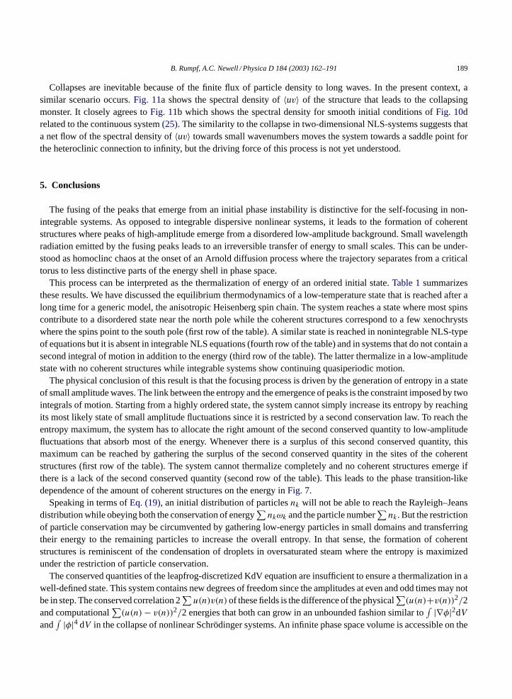
B. Rumpf, A.C. Newell / Physica D 184 (2003) 162–191 189
Collapses are inevitable because of the finite flux of particle density to long waves. In the present context, asimilar scenario occurs. Fig. 11a shows the spectral density of 〈uv〉 of the structure that leads to the collapsingmonster. It closely agrees to Fig. 11b which shows the spectral density for smooth initial conditions of Fig. 10drelated to the continuous system (25). The similarity to the collapse in two-dimensional NLS-systems suggests thata net flow of the spectral density of 〈uv〉 towards small wavenumbers moves the system towards a saddle point forthe heteroclinic connection to infinity, but the driving force of this process is not yet understood.
5. Conclusions
The fusing of the peaks that emerge from an initial phase instability is distinctive for the self-focusing in non-integrable systems. As opposed to integrable dispersive nonlinear systems, it leads to the formation of coherentstructures where peaks of high-amplitude emerge from a disordered low-amplitude background. Small wavelengthradiation emitted by the fusing peaks leads to an irreversible transfer of energy to small scales. This can be under-stood as homoclinc chaos at the onset of an Arnold diffusion process where the trajectory separates from a criticaltorus to less distinctive parts of the energy shell in phase space.
This process can be interpreted as the thermalization of energy of an ordered initial state. Table 1 summarizesthese results. We have discussed the equilibrium thermodynamics of a low-temperature state that is reached after along time for a generic model, the anisotropic Heisenberg spin chain. The system reaches a state where most spinscontribute to a disordered state near the north pole while the coherent structures correspond to a few xenochrystswhere the spins point to the south pole (first row of the table). A similar state is reached in nonintegrable NLS-typeof equations but it is absent in integrable NLS equations (fourth row of the table) and in systems that do not contain asecond integral of motion in addition to the energy (third row of the table). The latter thermalize in a low-amplitudestate with no coherent structures while integrable systems show continuing quasiperiodic motion.
The physical conclusion of this result is that the focusing process is driven by the generation of entropy in a stateof small amplitude waves. The link between the entropy and the emergence of peaks is the constraint imposed by twointegrals of motion. Starting from a highly ordered state, the system cannot simply increase its entropy by reachingits most likely state of small amplitude fluctuations since it is restricted by a second conservation law. To reach theentropy maximum, the system has to allocate the right amount of the second conserved quantity to low-amplitudefluctuations that absorb most of the energy. Whenever there is a surplus of this second conserved quantity, thismaximum can be reached by gathering the surplus of the second conserved quantity in the sites of the coherentstructures (first row of the table). The system cannot thermalize completely and no coherent structures emerge ifthere is a lack of the second conserved quantity (second row of the table). This leads to the phase transition-likedependence of the amount of coherent structures on the energy in Fig. 7.
Speaking in terms of Eq. (19), an initial distribution of particles nk will not be able to reach the Rayleigh–Jeansdistribution while obeying both the conservation of energy
∑nkωk and the particle number
∑nk. But the restriction
of particle conservation may be circumvented by gathering low-energy particles in small domains and transferringtheir energy to the remaining particles to increase the overall entropy. In that sense, the formation of coherentstructures is reminiscent of the condensation of droplets in oversaturated steam where the entropy is maximizedunder the restriction of particle conservation.
The conserved quantities of the leapfrog-discretized KdV equation are insufficient to ensure a thermalization in awell-defined state. This system contains new degrees of freedom since the amplitudes at even and odd times may notbe in step. The conserved correlation 2
∑u(n)v(n) of these fields is the difference of the physical
∑(u(n)+v(n))2/2
and computational∑
(u(n) − v(n))2/2 energies that both can grow in an unbounded fashion similar to∫ |∇φ|2dV
and∫ |φ|4 dV in the collapse of nonlinear Schrödinger systems. An infinite phase space volume is accessible on the

190B
.Rum
pf,A.C
.New
ell/Physica
D184
(2003)162–191
Table 1Summary of the thermalization processes of the Heisenberg spin chain, the discrete nonlinear Schrödinger equation, and the leapfrog map
Integrals of motion Initial conditions Phenomena Path to maximum entropy
(1) HamiltonianH, (2)M (magnetization)or N (particle number) due to rotationalsymmetry (Section 2.1.3)
Long waves with small amplitudes lowratio 〈H〉/〈N〉
Formation of coherent structures andlow-amplitude fluctuations (Figs. 1–3a, band 6a)
Transfer of 〈N〉 into coherent structuresoptimum ratio of 〈H〉/〈N〉 in fluctuations(Figs. 13a and 14a)
(1) HamiltonianH, (2)M or N due torotational symmetry (Section 2.1.3)
Short waves with small amplitudes andhigh 〈H〉/〈N〉; coherent structures withlow 〈H〉/〈N〉
Destruction of coherent structures (Fig. 3c) Transfer of 〈N〉 from coherent structuresinto fluctuations; decrease of 〈H〉/〈N〉 influctuations (Figs. 13a and 14b)
HamiltonianH, broken rotational symmetry(Section 3.3.4)
Any Disordered fluctuations (Fig. 6c and d) Production or reduction of 〈N〉 optimumratio of 〈H〉/〈N〉 in fluctuations
HamiltonianH, infinite number of integralsof motion (Section 3.3.3)
Any Quasiperiodic emergence of coherentstructures (Fig. 6b)
No thermalization
(1) Energy∑
uv, (2) mass∑
u,∑
v
(Section 2.2.2)k = 2π/3 waves with nonzero energy Formation of coherent structures and
low-amplitude fluctuations (Fig. 7a);‘monster’ (Fig. 10c)
Transfer of∑
uv into coherentstructures, heteroclinic connection toinfinity (Fig. 8)
(1) Energy∑
uv, (2) mass∑
u,∑
v
(Section 2.2.2)White noise with zero energy Sudden local growth of the amplitude
(Figs. 7b, 10a and b)Heteroclinic connection to infinity(Fig. 10c)

B. Rumpf, A.C. Newell / Physica D 184 (2003) 162–191 191
shells of constant∑
u(n)v(n). If∑
u(n)v(n) is finite (fifth row of the table), a modulational instability of usualBenjamin–Feir type leads to traveling soliton waves which sweep up smaller ones as they travel along the circleso that a scenario of merging peaks takes place on intermediate time scales. Finally, the system finds a way toexploit all of the phase space when a long wave instability of the background noise gives rise to the rapidly growing‘monster’ solution. The same solution can be initiated by a short-wavelength instability for
∑u(n)v(n) = 0 (sixth
row of the table). This solution is the systems canonical way of exploiting the phase space associated with infinitelyhigh-amplitudes.
Acknowledgements
BR gratefully acknowledges support by a grant of German Academic Exchange Service (DAAD). ACN gratefullyacknowledges support from NSF grant DMS 0072803.
References
[1] P.L. Kelley, Phys. Rev. Lett. 15 (1965) 1005.[2] V.E. Zakharov, Zh. Eksp. Teor. Fiz. 62 (1972) 1745;
V.E. Zakharov, Sov. Phys. JETP 35 (1972) 908.[3] A.C. Newell, SIAM J. Appl. Math. 33 (1977) 1.[4] W. Briggs, A.C. Newell, T. Sarie, J. Comp. Phys. 51 (1983) 83.[5] V.E. Zakharov, A.B. Shabat, Zh. Eksp. Teor. Fiz. 61 (1971) 118;
V.E. Zakharov, A.B. Shabat, Sov. Phys. JETP 34 (1972) 62.[6] S. Dyachenko, V.E. Zakharov, A.N. Pushkarev, V.F. Shvets, V.V. Yankov, Zh. Eksp. Teor. Fiz. 96 (1989) 2026;
S. Dyachenko, V.E. Zakharov, A.N. Pushkarev, V.F. Shvets, V.V. Yankov, Sov. Phys. JETP 69 (1989) 1144.[7] S. Dyachenko, A.C. Newell, A. Pushkarev, V.E. Zakharov, Physica D 57 (1992) 96.[8] M.J. Ablowitz, B.M. Herbst, SIAM J. Appl. Math. 50 (1990) 339.[9] A.M. Morgante, M. Johansson, G. Kopidakis, S. Aubry, Physica D 162 (2002) 53.
[10] D.W. McLaughlin, C.M. Schober, Physica D 57 (1992) 447.[11] A. Calini, N.M. Ercolani, D.W. McLaughlin, C.M. Schober, Physica D 89 (1996) 227.[12] R. Jordan, B. Turkington, C.L. Zirbel, Physica D 137 (2000) 353.[13] K.O. Rasmussen, T. Cretegny, P.G. Kevrekidis, N. Gronbech-Jensen, Phys. Rev. Lett. 84 (2000) 3740.[14] B. Rumpf, A.C. Newell, Phys. Rev. Lett. 87 (2001) 54102.[15] M.J. Ablowitz, J.F. Ladik, J. Math. Phys. 16 (1975) 598.[16] A.M. Kosevich, B.A. Ivanov, A.S. Kovalev, Phys. Rep. 194 (1990) 117;
B. Rumpf, H. Sauermann, Phys. Rev. E 58 (1998) 1463.[17] N.J. Zabusky, M.D. Kruskal, Phys. Rev. Lett. 15 (1965) 240.[18] A. Cloot, B.M. Herbst, J. Comp. Phys. 75 (1988) 31.[19] J.A. Krumhansl, J.R. Schrieffer, Phys. Rev. B 11 (1975) 3535;
K. Nakamura, T. Sasada, J. Phys. C 11 (1978) 331.[20] A.C. Newell, D.A. Rand, D. Russell, Physica D 33 (1988) 281.