plants and fibonacci - university of...

DOI: 10.1007/s10955-005-8665-7Journal of Statistical Physics, Vol. 121, Nos. 5/6, December 2005 (© 2005)

Plants and Fibonacci

Alan C. Newell1 and Patrick D. Shipman2

Received December 27, 2004; accepted June 15, 2005

The universality of many features of plant patterns and phyllotaxis has mys-tified and intrigued natural scientists for at least four hundred years. It isremarkable that, to date, there is no widely accepted theory to explain theobservations. We hope that the ideas explained below lead towards increasedunderstanding.

KEY WORDS: Pattern formation; phyllotaxis.

1. INTRODUCTION

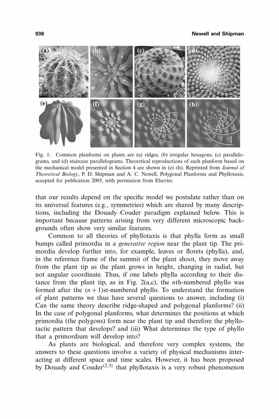
Since the time of Johannes Kepler, natural scientists have been fascinatedand intrigued by the observation that the phylla (elements such as leaves,florets, stickers or bracts) on many plants are arranged in such a mannerthat each phyllo lies on three familes of spirals. Moreover, the numbers ofarms in each of the spiral families are, in almost 95% of all cases, sequen-tial triads in the regular Fibonacci sequence 1,1,2,3,5,8, . . . (Fig. 2(a)).Further, the surfaces of these plants are tiled in polygonal shapes. Thechallenge is to provide a rational basis for understanding plant patterns,including an explanation for the presence of Fibonacci sequences.

By plant patterns we mean both the arrangement of phylla on plants(phyllotaxis) and the tiling of the plant surface into polygonal shapes suchas ridges, hexagons, or parallelograms; see Fig. 1. In recent work,(15,16) wehave suggested that much of what is observed can be explained by mini-mizing the elastic energy of a curved annular region of the plant’s tunica(outer skin) in the neighborhood of the shoot apical meristem (SAM). Inthis paper, we seek to address in more depth the question as to the extent

1Department of Mathematics, University of Arizona, Tucson, AZ 85721; e-mail: [email protected]

2Max Planck Institut fur Mathematik in den Naturwissenschaften, Inselstrasse 22, D-04103Leipzig, Germany; e-mail: [email protected]

937

0022-4715/05/1200-0937/0 © 2005 Springer Science+Business Media, Inc.

938 Newell and Shipman

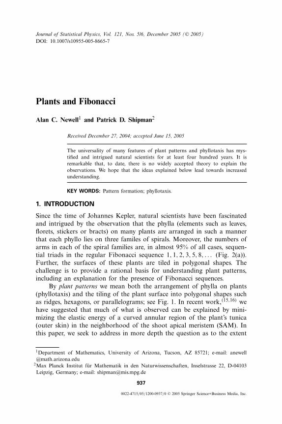
Fig. 1. Common planforms on plants are (a) ridges, (b) irregular hexagons, (c) parallelo-grams, and (d) staircase parallelograms. Theoretical reproductions of each planform based onthe mechanical model presented in Section 4 are shown in (e)–(h). Reprinted from Journal ofTheoretical Biology, P. D. Shipman and A. C. Newell, Polygonal Planforms and Phyllotaxis,accepted for publication 2005, with permission from Elsevier.

that our results depend on the specific model we postulate rather than onits universal features (e.g., symmetries) which are shared by many descrip-tions, including the Douady–Couder paradigm explained below. This isimportant because patterns arising from very different microscopic back-grounds often show very similar features.

Common to all theories of phyllotaxis is that phylla form as smallbumps called primordia in a generative region near the plant tip. The pri-mordia develop further into, for example, leaves or florets (phylla), and,in the reference frame of the summit of the plant shoot, they move awayfrom the plant tip as the plant grows in height, changing in radial, butnot angular coordinate. Thus, if one labels phylla according to their dis-tance from the plant tip, as in Fig. 2(a,c), the nth-numbered phyllo wasformed after the (n+ 1)st-numbered phyllo. To understand the formationof plant patterns we thus have several questions to answer, including (i)Can the same theory describe ridge-shaped and polygonal planforms? (ii)In the case of polygonal planforms, what determines the positions at whichprimordia (the polygons) form near the plant tip and therefore the phyllo-tactic pattern that develops? and (iii) What determines the type of phyllothat a primordium will develop into?

As plants are biological, and therefore very complex systems, theanswers to these questions involve a variety of physical mechanisms inter-acting at different space and time scales. However, it has been proposedby Douady and Couder(2,3) that phyllotaxis is a very robust phenomenon

Plants and Fibonacci 939

Fig. 2. The phylla of a cactus (a) and a succulent (c) are numbered according to their dis-tance from the center. In (a), lines are drawn connecting neighboring phylla; this producesfamilies of 3 (in black) and 8 (in grey) sets of clockwise spirals and a family of 5 (in white)counterclockwise spirals. (b,d) Putting radial r and angular α coordinates on the plant tipand defining s = r or s = ln(r), depending on if the plant exhibits the plastochrone differenceor ratio (see text), the numbered points form lattices in the (s, α)-plane. The vectors ωj arenatural choices as generating vectors for the lattices. Reprinted from Journal of TheoreticalBiology, P. D. Shipman and A. C. Newell, Polygonal Planforms and Phyllotaxis, accepted forpublication 2005, with permission from Elsevier.

and that many, if not most, of what is observed can be explained by asimple set of dynamical rules formulated by Hofmeister(13) or Snow andSnow(17)–that is, the answer to question (ii) is independent of the physi-cal mechanism responsible for producing primordia as long as the mecha-nism satisfies a few basic criteria. The central idea of Hofmeister, set outin Section 3, is that each new primordium should be placed in the most


“open” space available to optimize its ability to grow into fully maturedphylla. Douady and Couder constructed an experimental paradigm forthese rules in which a set of repelling points (which represent primordia)are introduced at fixed time intervals at the center of a plate.

Our picture is radically different. We do not suggest that individualprimordia are formed to optimize their own individual growth progress,but rather that the pattern that forms is a global one and that plant sur-faces in the generative region are, to a good approximation, linear com-binations

∑Nj=1 aj cos(lj r +mjα) of elementary periodic deformations, i.e.,

modes cos(lj r + mjα), where r and α are respectively radial and angularcoordinates centered at the summit of the plant tip. The choices of wave-vectors �kj = (lj ,mj ) and real amplitudes aj are determined by the physi-cal mechanism and minimize, in our physical model, the elastic energy ofa curved, elastic annulus (the generative region) under mechanical stresses(due to growth). We suggest that, while some general features of the phyl-lotactic pattern can be captured by members of a general class of modelssharing Hofmeister and/or Snow or Snow rules, there are other featureswhich are only captured by specific properties of the elastic sheet model.Further, we note that the interplay between stresses in the plant’s tunica,changes in the microstructure of the biological material and growth hor-mones (e.g., auxin), which play crucial roles in the later development offully mature phylla, is important, but for the first approximation our pic-ture suggests that the deformed surface is produced by purely mechanicalmeans. This model follows the pioneering work of Paul Green and his col-leagues at Stanford who argued, in the 1990’s, that various growth processeslead to compressive stresses in the plant’s tunica in an annular zone nearits shoot apical meristem. In a series of papers, they gave detailed reasonsand provided experimental evidence to support this picture.(9–12,18) Whatthey did not recognize was how crucial the quadratic nonlinear interactionsof the linearly most unstable modes are in the competition for dominance.These interactions lead naturally to most, if not all, of the phyllotactic pat-terns observed. They arise from that part of the in-place strain energy whichis the product of the perturbed Airy stress and the Gaussian curvature ofthe deformed surface, and the key observation is that this energy is mini-mized by special triads of modes whose wavevectors satisfy the condition�k1 + �k2 = �k3. By “special triads” we mean that the preferred wavevectors arethose that maximize a combination of their linear growth rates σ(�kj ) and aninteraction coefficient τ(�k1, �k2, �k3 = �k1 + �k2). Both σ and τ contain specificinformation regarding the physical mechanism.

Our goal in this short paper is to use comparisons with the Douady–Couder paradigm and the results of their energy functional based on


mutually repelling primordia in order to argue in favor of the Greenmodel which starts from premises which are well supported by experiment.The description of phyllotaxis in terms of phyllotaxis coordinates is pre-sented in Section 2. In Section 3 we delineate the premises and give themain results of the DC model. We write the premises of our biomechan-ical model in a parallel format in Section 4.1. In Section 4.2, we dis-cuss the growth (σ(l,m)) and interaction (τ ) coefficients and show that,as the plant grows, the energy-minimizing configuration evolves due tocombinations of a new, most linearly unstable circumferential mode andthe influence of already formed configurations which have moved out ofthe generative region. In Section 5, we discuss how the key difference ofour model from the DC paradigm—that the mechanical model leads to astudy of the interaction of elementary modes and the calculation of theiramplitudes, whereas the Douady–Couder paradigm assumes the interac-tion of primordia—allows us to address both questions (i) and (ii) and haspotential consequences for question (iii).

2. PHYLLOTACTIC PARAMETERS

In this section, we find the natural coordinates in which to statethe position of phylla on a plant and thus to describe phyllotaxis. InFig. 2(a,c), phylla are numbered according to their distance from the cen-ters of the plants. This allows us to illustrate the following three standardparameters used to describe phyllotactic patterns:

1. The whorl number g: Each phyllo on a plant is a member of awhorl of g phylla that are evenly spaced about a circle centered at thecenter of the plant. The number g is locally constant. For the example ofFig. 2(c), g = 2, as one sees pairs of phylla that are equidistant from thecenter of the plant. For the cactus of Fig. 2(a), g =1.

2. The divergence angle D = 2πd: The angle between consecutivelynumbered phylla is taken to be the angle between the rays from the centerof the plant to the centers of those phylla; see Fig. 2(a). It is an obser-vation that the angle between any two consecutively numbered phylla islocally constant on any plant; this constant is called the divergence angle,D = 2πd. There is a natural ambiguity in the measurement of the angle,as one can either measure clockwise or counterclockwise. If the two mea-surements are not equal, the plant shows a handedness and D = 2πd istaken to be the smaller of the two measurements; thus, 0 <d � 1

2 . In ourFig. 2(a) example, the divergence angle is roughly D = 2π(0.382) mea-sured clockwise, and for the example of Fig. 2(c), D = 2π

4 measured eithercounterclockwise or clockwise.


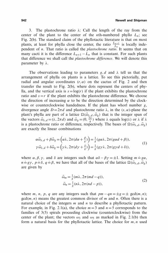
3. The plastochrone ratio λ: Call the length of the ray from thecenter of the plant to the center of the nth-numbered phyllo Ln; seeFig. 2(b). The standard claim of the phyllotactic literature is that on mostplants, at least for phylla close the center, the ratio Ln+1

Lnis locally inde-

pendent of n. That ratio is called the plastochrone ratio. It seems that onmany cacti it is the difference Ln+1 −Ln that is constant. For such plantsthat difference we shall call the plastochrone difference. We will denote thisparameter by λ.

The observations leading to parameters g, d and λ tell us that thearrangement of phylla on plants is a lattice. To see this pictorially, putradial and angular coordinates (r, α) on the cactus of Fig. 2 and thentransfer the result to Fig. 2(b), where dots represent the centers of phy-lla, and the vertical axis is s = log(r) if the plant exhibits the plastochroneratio and s = r if the plant exhibits the plastochrone difference. We choosethe direction of increasing α to be the direction determined by the clock-wise or counterclockwise handedness. If the plant has whorl number g,divergence angle D =2πd and plastochrone ratio λ, in the (s, α)-plane theplant’s phylla are part of a lattice �( �ωλ,d, �ωg) that is the integer span ofthe vectors �ωλ,d = (λ,2πd) and �ωg = (0, 2π

g) where λ equals log(λ) or λ if λ

is a plastochrone ratio or difference, respectively. The bases of �( �ωλ,d, �ωg)

are exactly the linear combinations

α �ωλ,d +β �ωg =(αλ,2π(dα + β

g))

= 1g(gαλ,2π(gαd +β)),

γ �ωλ,d + δ �ωg =(γ λ,2π(dγ + δ

g))

= 1g(gγ λ,2π(gγ d + δ)),

(1)

where α,β, γ, and δ are integers such that αδ −βγ =±1. Setting m.=gα,

n.=gγ , p

.=δ, q.=β, we have that all of the bases of the lattice �( �ωλ,d, �ωg)

are given by

�ωm = 1g(mλ,2π(md −q)),

�ωn = 1g(nλ,2π(nd −p)),

(2)

where m, n, p, q are any integers such that pm− qn=±g =± gcd(m,n);gcd(m,n) means the greatest common divisor of m and n. Often there is anatural choice of the integers m and n to describe a phyllotactic pattern.For example, in Fig. 2.1(a), the choice m=3 and n=5 corresponds to thefamilies of 3(5) spirals proceeding clockwise (counterclockwise) from thecenter of the plant; the vectors ω3 and ω5 as marked in Fig. 2.1(b) thenform a natural basis for the phyllotactic lattice. The choice for m,n used


to describe the pattern is referred to as the parastichy pair. The choiceof parastichy pair used to describe a pattern has some degree of ambigu-ity; for example, the eight clockwise spirals of Fig. 2.1(a) justify a possiblechoice of (5,8). For lattices with g >1, spirals are not as easily traced outby the eye. We will take the convention of stating the choice (m,n)= (g, g)

as the parastichy pair for such a pattern; the corresponding lattice gener-ators (2) are marked as ω2 and ω′

2 in Fig. 2.1(d).It is observed in plants that the Fibonacci sequence arises as the par-

astichy pair of a phyllotactic pattern undergoes transitions, starting withlower numbers such as (m,n) = (1,2) or (m,n) = (2,3) and moving upthe sequence 1,2,3,5,8, . . . (i.e., (1,2) → (2,3) → (3,5) → ·· · ), typicallyas the plant grows in width. These transitions arise in both our modeland that of DC as continuous (second order, Type II) transitions. Transi-tions in which the parastichy pair moves up the sequence (2,2)→ (2,3)→(3,3) → ·· · are also observed in nature and arise as discontinuous (firstorder, Type I) transitions in the models.

3. HYPOTHESES OF HOFMEISTER AND THE SNOWS, AND THE

DOUADY–COUDER PARADIGM

Phylla are only formed near the tip of a plant, so that the phyllotacticpatterns as seen in Fig. 2 are the result of a prolonged process in whichphylla form and then move away from the plant tip as the shoot growsin height. This process is described by three of five rules formulated byWilhelm Hofmeister in 1868. As stated by Douady and Couder,(12) theserules are

1. The stem apex (Fig. 3) is axisymmetric.

2. The primordia are formed at the periphery of the apex (Region 2in Fig. 3) and, due to the shoot’s growth, they move away from the centerwith a radial velocity V (r) which may depend on their radial location.

The next two Hofmeister rules concern the determination of the posi-tions at which the primordia form, i.e. the choice of divergence angle 2πd.These will be stated in the next section. The last Hofmeister rule reads

5. Outside of a region of radius R (Region 3 of Fig. 3), there is nofurther reorganization leading to changes in the angular position of theprimordium.

Our discussion now will focus on what belongs in slots 3. and 4.–whatdetermines if and where primordia are formed in the generative region.


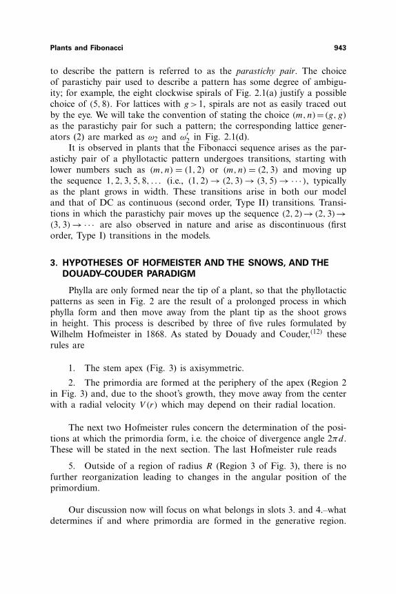
Fig. 3. Schematic representation of the shoot apical meristem (SAM). The SAM consists ofa thin skin (the tunica, Regions 1,2,3 in the diagram) attached to a foundation of less wellorganized cells (the corpus, Region 4 in the diagram). Cells in Region 1 show little growthactivity and Region 2 is the generative region in which active cell division is occuring andnew primordia are first seen to form. As the plant tip grows, cells move from Region 2 toRegion 3, radially outward in the reference frame of the diagram’s north pole. In Region 3,primordia that formed in Region 2 further develop into mature elements such as leaves. InSection 4, radial r and angular α coordinates on the tunica surface in the generative regionare defined by projecting the surface to the polar coordinates on the plane. Reprinted fromJournal of Theoretical Biology, P. D. Shipman and A. C. Newell, Polygonal Planforms andPhyllotaxis, accepted for publication 2005, with permission from Elsevier.

Concerning positions at which primorida form in the generative region,Hofmeister proposed the rules

3. New primordia are formed at regular time intervals (the plastoch-rone T ).

4. The incipient primordium forms in the largest space available leftby the previous ones.

Douady and Couder (DC) sought the simplest experiment that couldsimulate the Hofmeister rules. Their basic experimental device is a platewith a small central dome in the mddle; this is to represent to the plantwith the apex at the tip. The plate is placed in a vertical magnetic fieldthat is stronger at the edges of the plate than in the middle, and ferro-magnetic drops (representing primordia) are periodically dropped onto thecenter of the central dome (representing the apex). The drops fall to theperimeter of the central dome and then move radially outward, followingthe gradient of increasing magnetic strength. The magnetic field is chosenso that the velocity V (r) in an exponentially increasing function of theradius. After choosing a radial direction in which to fall from the top


of the central dome, the drops do not change their angular coordinate.How the drops initially choose their angular coordinate is of interest, andhere the central point is that the drops form repelling magnetic dipoles. Adrop that falls on the central dome moves to the position on the bound-ary of the dome as determined by the repulsions of the drops that recentlyformed and are moving away from the center, and the experimental resultis that a there is constant divergence angle between the angular coordi-nates of successively-dropped drops. Denoting the radius of the centraldome by R, the initial speed of the drops after falling to the boundaryof the dome by V0, and the time period in which drops are dropped ontothe central dome by T , the plastochrone ratio of the resulting pattern isG

.= V0TR

. G is a parameter chosen by the experimenter. As Douadyand Couder decrease G, the divergence angle between succesive dropsapproaches the golden angle and a lattice pattern with a Fibonacciparastichy pair is produced.

As the Hofmeister rules (3) and (4) and the electromagnetic paradigmassume that one primordium forms at a time, the Hofmeister rules do notallow for the formation of whorl patterns with g > 1 as in Fig. 2(c). DCthus turned to a revised set of hypotheses of Snow and Snow;(17) as statedby Douady and Couder,(4) the revised rules read

3. The apex is in the shape of a parabaloid, and the primordia canhave an azimuthally elongated shape.

4. A new primordium forms when and where a large enough spacehas been formed at the periphery of the apex.

The area of a primordium and the growth of the primordia and apexnow play central roles. DC imagine primordia as circles with diameter d0on a parabaloid with curvature described by a parameter N . For N = 1,the apex is flat, and for N > 1, the apex has curvature. Projected to theplane, the circular primordia on a curved apex will be elongated in theangular direction, so N > 1 can be thought of as describing azimuthally(angularly) elongated primordia. As a primordium of diameter d0 occupiesspace that can then not be taken by another primordium, DC imagine thateach primordium generates a repulsive energy E(d), where d is the dis-tance from the primordium. Projecting the apex parabaloid onto the planeand using polar coordinates, DC employ the distance function

d(P0, P1)=√√√√

[r2

0 − r21

N+2Nr0r1 (1− cos(θ0 − θ1))

]

. (3)


between two points with coordinates P0 = (r0, θ0) and P1 = (r1, θ1), and therepulsive energy that a primordium exerts on points a distance d from itis given by

E(d)=−1+

(tanh α d

d0

)−1

−1+ (tanh α)−1. (4)

Here α is a “stiffness” parameter; for lower α, a primordium has a largerinfluence on other points. Thus, any point on the generative circle ofradius R from the apex summit has a repulsive energy exerted on it byeach of the previously formed primordia that have since moved radiallyoutward. The energy E(θ) of a point P = (R, θ) on the generative circleis defined to be the sum of the repulsive energies exerted on that pointby each of the previously formed primordia. As the primordia move out-ward, the energy E(θ) decreases at any point. DC show that it is equiva-lent to say that a space of diameter d0 (and therefore a potential spot fora new primordium to form on the generative radius) has formed as it isto say that the energy E(θ) becomes lower than some threshold value atthat point. Thus, to simulate the Snow and Snow hypothesis 4., DC allowa primordium to form on the generative circle where and whenever E(θ)

decreases to the threshold value. In numerical experiments, DC investigatethe phyllotactic patterns that form as the parameter �= d0

Rdecreases. They

employed two schemes. In the first scheme, starting from a large valueof �, they let n consecutive particles appear, where n was large enoughto allow for a steady-state regime to appear and varied from up to 150to 500. Then, starting from the positions of the last approximately 20deposited primordia, they decreased � a small amount and let particlesform again until a steady-state regime was found. For the second scheme,DC began with a few primordia having a configuration that was expectedto be either stable or unstable and observed whether or not the patterncontinued to grow.

The main geometric parameter that determines the pattern that devel-ops is the ratio �, which plays a role analogous to that of G in the electro-mechanical paradigm. Both whorled and spiral phyllotactic arrangementsof primordia were produced in the numerical experiments, with largerparastichy numbers for smaller values of �, and to simulate a typicalplant, DC sought to understand what happens as � decreases from a largevalue.

1. For large values of �, the relative stability of the whorled and spi-ral modes is determined by the conicity N and stiffness α parameters.The decussate (alternating 2-whorl) (2,2,4) configuration could only be


obtained for large values of the conicity parameter N . The explorationof various values of α showed that large values of α (i.e., short-rangeinteractions) favor whorled modes, whereas small values favor spiralmodes. Thus, in the DC model, the whorled decussate mode (2,2) canonly exist at large � with either azimuthally elongated primordia orwith conical apices and short-range interaction.

2. As � is decreased, Type I transitions in which the parastichy num-bers increase up the sequence (n − 1, n) → (n, n) → (n, n + 1) → ·· · areobserved. However, the transition between, for example, a (1,2,(3)) spi-ral state and a (2,2,(4)) decussate state is not abrupt; in between thereis a transitory state in which the divergence angle varies periodically.

3. For low �, Type I transitions to whorled modes of higher order con-tinue to occur. To produce Type II transitions and therefore spiral pat-terns, DC take �(t) as a rapid function of time. The system then doesnot have enough time at a given value of � to make a transition to awhorled mode, and a continuous change (m,n)→ (n,m+n) to the nextspiral mode occurs.

The DC model is thus able to capture both whorled and spiral phyl-lotaxis, with transitions between patterns determined by the evolution of�. The suggestion of DC is that any microscopic mechanism must con-tain the simple dynamial rules of their model in that it (1). defines finite-sized primordia and (2). allows for an interaction (repulsion or attraction)of the primordia.

By assuming that primordia of a given shape form, the Douady–Couderparadigm focuses on the phyllotactic question (ii). In the case of polygonalplanforms, what determines the positions at which primordia (the polygons)form near the plant tip and therefore the phyllotactic pattern that develops?Thus, the formation of ridges and various polygonal configurations such ashexagons and parallelograms are not captured by their model.

4. BIOMECHANICAL MODEL

4.1. Justification for and Hypotheses of a Biomechanical Model

Our goal now is to formulate a biomechanical model for the forma-tion of plant patterns. Green, et al. have provided the following evidencethat a biomechanical mechanism underlies the plant pattern formation:

1. Hernandez and Green(12) grew a sunflower head between two fixed par-allel bars. This resulted in an amplification of undulations parallel tothe bars, and phyllotaxis followed this pattern. This external mechani-cal influence also changed the identity of the sunflower bracts.


2. Green(9) induced a new row of leaves to form on an expanding meri-stem by using a glass frame to apply a mechanical constraint.

3. Steele(18) noted that the turgor pressure inside plant cells is between 7and 10 atmospheres, and that this large pressure can hardly be ignoredin the phyllotactic process. Also, in this paper, Steele notes a linear rela-tionship between the size of primordia and the thickness of the tunica.

4. In,(5) Dumais and Steele showed sunflowers cut along a diameter. Thetwo sides of the cut stick together only in the region of the surfacewhere the pattern formation is occurring, indicating that the compres-sive force keeping the cut closed is related to the pattern formation.

5. Fleming et al.(7) were able to induce primordia on tomato plants bylocally applying the protein expansin; some of these primordia thendeveloped into leaf-like structures. The known effect of the extracellu-lar expansin proteins is to increase cell wall extensibility, thus changingthe mechanical properties of the plant material.

In the review article(9) Green outlines the hypothesis that bucklingof the compressed tunica is the main mechanism determining phyllotac-tic pattern. Green continues to discuss evidence for feedback mechanismsbetween the buckling configuration and changes in cellulose orientation incell walls and direction in cell division; buckling is thus only one com-ponent in the complex process of building the pattern, and it is interest-ing to note that similar feedback mechanisms between changes in stressesand changes in cellulose orientation have been noted for wood cells in treebranches.(6,19) However, the hypothesis of Green is that the reasons forFibonacci patterns and the difference between Types I and II transitionscan be found within the buckling mechanism.

The first three hypotheses of our model are modeled on the first threehypotheses of Snow and Snow as stated by DC. They read

1. The stem is axisymmetric.2. A normal deflection w of the generative region at the periphery of the

apex is produced and advected out in the reference frame of the apexsummit.

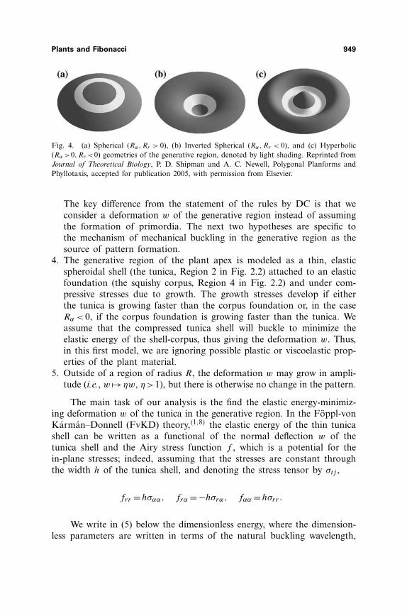
3. The curvature of the annular generative region can be described bysigned radii of curvature Rα and Rr in the angular and radial direc-tions, with Rj taken to be positive if the surface along the j coordinateline bends away from the normal vector (see Fig. 4). In this article, weassume that Rα =Rr so that the curvature of the generative region is aspictured in either Fig. 4 (a) or (b), depending on the sign of Rα. Moregeneral shapes are included in,(16) but are not essential for our argu-ment. The coordinates r and α are placed on the annular generativeregion by projection to the polar coordinates on the plane; see Fig. 4.


Fig. 4. (a) Spherical (Rα,Rr > 0), (b) Inverted Spherical (Rα,Rr < 0), and (c) Hyperbolic(Rα >0,Rr <0) geometries of the generative region, denoted by light shading. Reprinted fromJournal of Theoretical Biology, P. D. Shipman and A. C. Newell, Polygonal Planforms andPhyllotaxis, accepted for publication 2005, with permission from Elsevier.

The key difference from the statement of the rules by DC is that weconsider a deformation w of the generative region instead of assumingthe formation of primordia. The next two hypotheses are specific tothe mechanism of mechanical buckling in the generative region as thesource of pattern formation.

4. The generative region of the plant apex is modeled as a thin, elasticspheroidal shell (the tunica, Region 2 in Fig. 2.2) attached to an elasticfoundation (the squishy corpus, Region 4 in Fig. 2.2) and under com-pressive stresses due to growth. The growth stresses develop if eitherthe tunica is growing faster than the corpus foundation or, in the caseRα < 0, if the corpus foundation is growing faster than the tunica. Weassume that the compressed tunica shell will buckle to minimize theelastic energy of the shell-corpus, thus giving the deformation w. Thus,in this first model, we are ignoring possible plastic or viscoelastic prop-erties of the plant material.

5. Outside of a region of radius R, the deformation w may grow in ampli-tude (i.e., w �→ηw, η>1), but there is otherwise no change in the pattern.

The main task of our analysis is the find the elastic energy-minimiz-ing deformation w of the tunica in the generative region. In the Foppl-vonKarman–Donnell (FvKD) theory,(1,8) the elastic energy of the thin tunicashell can be written as a functional of the normal deflection w of thetunica shell and the Airy stress function f , which is a potential for thein-plane stresses; indeed, assuming that the stresses are constant throughthe width h of the tunica shell, and denoting the stress tensor by σij ,

frr =hσαα, frα =−hσrα, fαα =hσrr .

We write in (5) below the dimensionless energy, where the dimension-less parameters are written in terms of the natural buckling wavelength,


namely the length of the most linearly unstable mode. The natural wave-length is given by 2π�, where

�4 = Eh3ν2

κ + Eh

R2α

,

for Young’s modulus E, Poisson’s ratio ν and the Hooke’s constant κ ofthe elastic foundation. Two parameters in the energy express the geometryof the generative region and two give the stress tensor.

The first geometric parameter is the ratio

� = R

�

of the circumfrance 2πR of the central circle in the generative regionto the natural wavelength 2π�; this is roughly the inverse of the DCparameter � and will play an analogous role in our model. Approximatingthe Laplacian by the Euclidean Laplacian � = ∂2

r + 1�2 ∂2

α (instead of theLaplacian ∂2

r + 1�∂r + 1

�∂2α we simplify the analysis; notice that this simplifi-

cation is similar to that used by DC in that it is valid if pattern formationis determined by what happens on the circle of radius R. Assuming thatthe two radii of curvature in the generative region are of equal magnitude(so the apex is spherical; more general shapes are discussed in ref. 18), thesecond geometric parameter expresses the dimensionless curvature

C = �2

Rαhν

of the apex in the generative region. This is analogous to the DC conici-ty parameter N , but notice that, whereas C is strictly relevant at radius R

from the apex summit where new primordia are forming, the parameter N

expresses the conicity of the entire apex and is essential for determing theeffect of old primordia on newly formed primordia.

Experimental evidence indicates that the largest compressive stress inthe generative region is along the angular coordinate line;(5) the principlestresses (averaged through the width of the shell) are thus Nrr =hσrr andNαα =hσαα. The corresponding dimensionless parameters are

P =−Nαα�2

Eh3ν2, χ = Nrr

Nαα

.

Scaling the radial coordinate by 2π�, the dimensionless elastic energyfunctional is given by


E(w,f )=∫

⎡

⎣12 (�w)2+V (w) −1

2P(χ∂rw+ 1

�2 ∂αw)2

+f(C�w− 1

2ν�2 [w,w])

− 12 (�f )2

⎤

⎦dr dα,

(5)

where [f,w] = frrwαα + fααwrr − 2frαwrα, and consists of the followingterms: The first term in (5) resists buckling and corresponds to the bend-ing energy of the shell. V (w) is a potential coming from the elastic foun-dation and an applied pressure from corpus growth; we take V (w) =κ2 w2 + γ

4 w4 for spring constants κ and γ . The next two terms are a strainenergy, approximately equal to the Airy stress function multiplied by theGaussian curvature.(7) The final term arises from in-surface deformations.The dimensionless FvKD equations for an overdamped shell are the vari-ational equations ζwt =− δE

δw, 0=− δE

δf, so that, after scaling t ,

wt +�2w +κw +γw3 +P

(

χ∂2r w + 1

�2∂2αw

)

+C�f − 1ν�2

[f,w]=0,

�2f −C�w + 12ν�2

[w,w]=0. (6)

The first equation is the stress equilibrium equation, and the second givesa compatibility condition relating w and f . Note that the parameter � canbe hidden in the equations by scaling α �→ 1

�α.

When the stress P is larger than some critical value Pc, the uniformstatic solution w0 =0, f0 =−P(χr2 +α2) of the FvKD equations is linearlyunstable and certain shapes and configurations are preferentially ampli-fied. We write the deviations w(r,α, t) from w0 as

∑Nj=1(Aj (t)eilj r+imj α+

complex conjugate) and the deviations f (r, α, t) from f0 in terms of theAj(t) by solving iteratively the compatibility equation 0 = δE

δf. Substitut-

ing these expressions into (5) and averaging over space, the perturbationenergy E(w,f ) becomes

E = −∑

�k∈A

σj (lj ,mj )AjA∗j −

∑τ123

(A1A2A3 +A∗

1A∗2A

∗3

)

+N∑

c,d=1

γcdAcA∗cAdA∗

d . (7)

Details of the calculation are given in.(16) The first sum in (7) is taken overall wavevectors which are in the active set A, which is the set of �kj for


which the (real) linear growth rates σ(lj ,mj ) are greater than some smallnegative number (to allow for subcritical bifurcations). The cubic termsin (7) arise from all wavevector triads in A–that is, all triplets �k1, �k2, �k3of wavevectors in A such that �k1 + �k2 = �k3. The coefficient τ123(�k1, �k2, �k3 =�k1 + �k2), given below, is a function of the triad wavevectors. The quarticterms are positive definite and are mainly due to the elastic foundation(the squishy corpus). As the system is overdamped, the time dependenceof the Aj(t) are given by gradient flows ζ ∂

∂tAj = − δE

δA∗j, and therefore

{Aj(t)}N1 relax to local minima in E. Our task is to find energy-minimizingconfigurations.

As the energy-minimizing amplitudes Aj are found to be real num-bers, the energy-minimizing deformation w(r,α) = ∑N

j=1(Aj (t)eilj r+imj α+complex conjugate) can be written as w(r,α) = ∑

aj cos(�kj · �x), aj = 2Aj ,�x = (r, α). This energy-minimizing w(r,α) is the theoretical calculation forthe buckling pattern in the generative region. Assuming that the patternformed in the generative region remains the same as material moves radi-ally outward from the generative region (our hypotheses 2. and 5.), afterthe tip has grown a length rg, the observed pattern is given by the graphof the function w(s,α), 0 < s < rs , where s = r, rs = rg or s = ln(r), rs =ln(rg), depending on if the radial growth is constant or exponential. Thisleads in the former case to a pattern with the plastochrone difference, andin the latter case to one with the plastochrone ratio.

It will convenient for the analysis in Section 4 to connect the defor-mation w(r,α) with the phyllotactic lattice generators 2 in the case when

w(r,α)=N∑

j=1

aj cos(�kj · �x), (8)

where the wavevectors �kj are integer combinations of two wavevectors�km = (lm,m) and �kn = (ln, n) (for example, if w(r,α) = ∑3

j=1 aj cos(�kj · �x),where �k1 + �k2 = �k3). The maxima of the deformation (8), where each wave-vector is an integer combination of

�km = (lm,m)=(

2π

λ(q −md),m

)

, �kn = (ln, n)=(

2π

λ(p −nd), n

)

,

(9)

for given choices of d, λ,m,n and p,q such that pm−qn=±g, occur ona lattice spanned by the generators of phyllotactic lattices given by (2),


namely

�ωm = 1g

(λm,2π(md −q)), �ωn = 1g

(λn,2π(nd −p)). (10)

The relationship between a pair of wavevectors (9) and the dual pair (10)of lattice generators can be expressed by defining the matrices

K=( �kn

�km

)

=( 2π

λ(p−nd) n

2πλ

(q−md) m

)

, �=(�ωm, �ωn)= 1g

(λm λn

2π(md−q) 2π(nd−p)

)

such that

K�=±2πI.

As the radial coordinate in (5) is scaled by the natural wavelength 2π�,the modulus A=2π λ

gR� of the determinant of the matrix

�′ = ( �ωm, �ωn)= 1g

(λ�m λ�n

2πR(md −q) 2πR(nd −p)

)

approximates the area of a newly formed primordium (ignoring the curva-ture of the apex in the generative region and assuming that the size of theprimordium is small compared to R).

4.2. Energy-Minimizing Configurations

4.2.1. The Most Unstable Mode; Ridge Planforms

The first task in minimizing the energy (7) is to determine the set Aof active modes and the properties of the coefficient σ(l,m). The lineargrowth of a mode with wavevector �k = (l,m) is

σ(l,m)=−(

l2 + 1�2

m2)2

+P

(

χl2 + 1�2

m2)

−1. (11)

The smallest value of P for which there is a mode with nonnegative lineargrowth is the critical value Pc =2, at which σ(l =0,m=�)=0. For P >Pc,there is a set of modes with positive linear growth rates, but the criticalwavevector �kc = (0,�) remains the mode with the largest linear growth rate.The derivation of the energy (7) assumes that the stress parameter P is


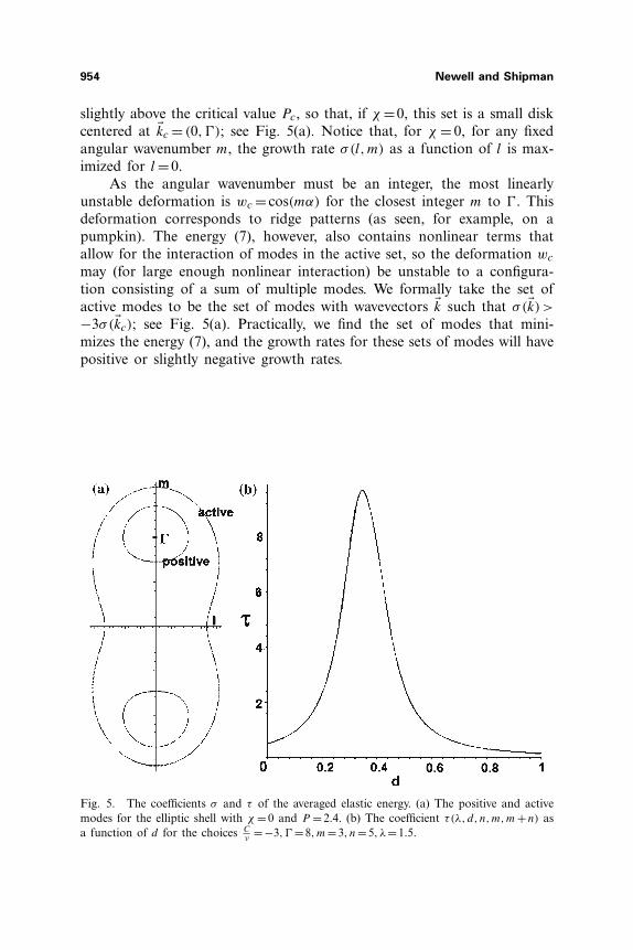
slightly above the critical value Pc, so that, if χ =0, this set is a small diskcentered at �kc = (0,�); see Fig. 5(a). Notice that, for χ = 0, for any fixedangular wavenumber m, the growth rate σ(l,m) as a function of l is max-imized for l =0.

As the angular wavenumber must be an integer, the most linearlyunstable deformation is wc = cos(mα) for the closest integer m to �. Thisdeformation corresponds to ridge patterns (as seen, for example, on apumpkin). The energy (7), however, also contains nonlinear terms thatallow for the interaction of modes in the active set, so the deformation wc

may (for large enough nonlinear interaction) be unstable to a configura-tion consisting of a sum of multiple modes. We formally take the set ofactive modes to be the set of modes with wavevectors �k such that σ(�k)>

−3σ(�kc); see Fig. 5(a). Practically, we find the set of modes that mini-mizes the energy (7), and the growth rates for these sets of modes will havepositive or slightly negative growth rates.

Fig. 5. The coefficients σ and τ of the averaged elastic energy. (a) The positive and activemodes for the elliptic shell with χ = 0 and P = 2.4. (b) The coefficient τ(λ, d, n,m,m+n) asa function of d for the choices C

ν=−3,� =8,m=3, n=5, λ=1.5.


4.2.2. The Most Unstable Triad; Hexagon Planforms

As the key nonlinear interaction is encoded in the cubic coefficient

τ(�kr , �ks, �kr+s = �kr + �ks)= τ(r, s, r + s) = − C

ν�2(lrms − lsmr)

2

×∑

j=r,s,r+s

1

l2j + 1

�2 m2j

, (12)

we first describe key characteristics of how τ depends on the parametersand choices of wavevectors.

0. As in σ , the angular wavenumber m and parameter � only appear in τ

in the ratio m�

. The parameter � can be scaled, through m, out of theenergy (7).

1. τ is proportional to the curvature constant C; when C =0 the quadraticcoefficient in the amplitude equations vanishes. This means that ridgesare the only stable solutions of the amplitude equations when C = 0.Note that the appearance of C in the amplitude equations comes fromthere being nonzero curvature in the original, unbuckled shell. τ is pos-itive for C < 0 (i.e., for the hyperbolic or inverted spherical generativeregion, Fig. 4 (b,c)) and negative for C > 0 (i.e., for the spherical gen-erative region, Fig. 4(a)).

2. As lrms − lsmr = lrmr+s − lr+smr = lsmr+s − lr+sms , τ(�kr , �ks, �kr+s) is asymmetric function of the wavevectors.

3. What values of the radial wavenumbers maximize τ ? For a fixed valueof mj , the fraction

1(l2j + 1

�2 m2j

)2

is maximized for lj = 0. If, however, two radial coordinates are equalto zero, then τ also equals 0 due to the factor (lrms − lsmr)

2. For fixedangular wavenumbers, the coefficient τ achieves local maxima at whereexactly one of the radial coordinates is zero.Writing the radial wavevectors in terms of the phyllotactic coordinates,τ(r, s, r + s) becomes

τ =−C

ν(2π)2

⎡

⎢⎢⎣

1

2π(�

q−mdg

)2+m2 λ2

g2

+ 1

2π(�

p−ndg

)2+n2 λ2

g2

+ 1

2π(�

p+q−(m+n)dg

)2+(m+n)2 λ2

g2

⎤

⎥⎥⎦ (13)


From this last expression, we see that the condition that exactly one ofthe radial coordinates is zero means that τ(m,n,m+n), as a function ofd, achieves local maxima at the three values d = p

n,

qm

,p+qm+n

that make oneof the radial coordinates equal to zero. In fact, τ is a very sensitive func-tion of d, as illustrated in the graph of τ as a function of d in Fig. 5(b).Also from (13) one sees that the coefficient τ is larger for smaller λ–thatis, for larger l1, l2.

4. What values of the angular wavenumbers maximize τ ? Writing �k1 =(l1,m3 − m), �k2 = (l2,m), �k3 = (l1 + l2,m3), fixed m3 and arbitrary val-ues of C and �, τ is maximized at m = |l2|m3

|l1|+|l2| . In particular, we willbe interested in the case l1 =−l2, �k3 = (0,m3 =�), for which τ is maxi-mized at �k1 = (l,

m32 ), �k2 = (−l,

m32 ).

We first assume for simplicity that � =2N for some integer N . Then,the most unstable mode as P increases above threshold has wavevector�kc = (0,� = 2N). However, for large enough τ(�km, �kn, �kc) this ridge solu-tion, with amplitude Ac = σ(0,2N)

3γ, can become unstable to a triad of

modes with wavevectors �km, �kn, �kc, where �km + �kn = �kc. The energy (5)allows for multiple triads, but as a first step we seek to find the mostunstable single triad configuration. Writing �km = (l,m)= 1

g( 2π

λ(q −md),m)

and �kn = (−l, n) = 1g( 2π

λ(p − nd), n), we need to determine what choices

of l m and n (or, equivalently, what choices of λ and d and m,n) andcorresponding amplitudes Am, An, Ac give the lowest energy single-triadconfiguration. The following points in this consideration correspond innumbering to the list of properties for τ .

0. The parameter � only affects the chosen triad through a scaling of theangular wavenumbers.

1. As τ is proportional to C, for C = 0, ridges (Ac = σ(�kc)3γ

, Am = 0 = An)are the only solution to the amplitude equations. For larger |C| thereare special triads for which τ is large enough for there to be a “hexa-gon” solution with all three amplitudes nonzero. For C <0 (the invertedsphere), the amplitudes are all positive, whereas for C >0 (the sphere),the amplitudes are all negative.

2. As τ is a symmetric function of the wavevectors, from the inequalityσ(�kc)>σ(�kn) for all wavevectors �kn in A follows the amplitude inequal-ity |Ac| > |An|. We will, in fact, find |Ac| > |Am| � |An|, with the ratio|An||Ac| increasing to 1 as |C| increases.

3. The linear growth rates σ(�km) and σ(�kn) are largest for m,n as closeas possible to � = 2N under the constraint m+n= 2N ; also, assumingthat τ =τ(�km, �kn, �kc = (0,2N)), τ is maximized for the choice m=n=N .


Numerical experiments give m=n=N as the energy-minimizing choiceof angular wavenumbers.

4. As �kc = (lc =0,2N), we have that �km = (l,m=N), �kn = (−l, n=N). Theretension between σ and τ as to the best choice of l; σ is maximized forl =0, whereas τ is maximized for l =∞. However, the critical wavenum-ber choice lc =0, i.e., d = p+q

m+n, is in the range of large τ even for small

choices of l. This allows for there to be a compromise choice, numer-ically determined to be l � 1 for χ = 0; larger values of χ give largervalues of l, but l remains near 1 for reasonable values of χ .

Hence, for � = 2N and large enough |C|, the energy-minimizingtriad configuration is w = ∑

j=m,n,m+n Aj cos(�kj · �x) with �km = (l,N), �kn =(−l,N), and �km+n = �kc = (0,2N) and with positive (respectively, negative)real Aj for C <0 (respectively, C >0). For � =2N +1, it is no longer pos-sible to choose m=n; in the energy-minimizing configuration, m=N,n=N + 1. Examples for � = 12 and C < 0 are shown in Fig. 1(a) and, forlarger |C|, in Fig. 1(b). For C > 0, the centers of the hexagons would bethe minima instead of the maxima of the configuration.

We next address the question of transitions between these configura-tions as the size of � increases. As � increases from 2N to 2N +1 and onup, the energy-minimizing triad changes in the sequence

�kN = (l,N) �kN = (l,N) �kN+1 = (l,N +1)�k′N = (−l,N) → �kN+1 = (−l,N +1) → �kN+1 = (−l,N +1) →·· · .

�k2N = (0,2N) �k2N+1 = (0,2N +1) �k2N+1 = (0,2(N +1))

(14)

As � increases from 2N to 2N +1 and then from 2N +1 to 2N +2, thereis an abrupt change in the optimal triad, but the triad always has theform �km = (l,m), �kn = (−l, n), �km+n = (0,m + n = �), where we find that l

does not depend on � (l is of order 1 and does depend on χ as discussedabove). Writing the wavevectors in the standard form �km = (lm = 2π

λ(q −

md),m), �kn = (ln = 2πλ

(p −nd), n), �km+n = ( 2πλ

(p + q − (m+n)d),m+n), wesee that �km+n = (0,�) implies that d = p+q

m+n= p+q

�, and therefore l = lm =

−ln = ±2πgλ

1�

. As l is constant with respect to �, the ratio gλ

changes

like �. As a consequence, the area A = 2π λgR� = 2π λ

g��2 = (2π�)2

lof a

primordium is constant with respect to �.These are transitions of Type I. As noted in Section 2, these transi-

tions are observed in nature, particularly on plants (e.g., saguaro cacti) forwhich the configuration is dominated by ridges (i.e., on plants for which|A1||A3| is small), although they can also be observed on plants with hexago-nal configurations, as in Fig. 6(a). Also note that one wavevector is pre-served in each transition of the sequence (14). If one draws the curves


Fig. 6. (a) On a plant that undergoes a Type I transition one observes two dislocations(black and grey lines) and a family of spirals (white lines) that has no defect. (b) A TypeI transition from a (2,2,4) alternating 2-whorl phyllotaxis (large values of s) to (2,3,5)-spiralphyllotaxis (small s) is drawn schematically. One spiral family (white lines) does not changeduring the transition. A penta-hepta pair is formed where the two dislocations in the otherspiral families meet. The corresponding wavevectors are illustrated in (c) and (d) along withthe typical boundary of the set of active modes. Reprinted from Journal of Theoretical Biol-ogy, P. D. Shipman and A. C. Newell, Polygonal Planforms and Phyllotaxis, accepted forpublication 2005, with permission from Elsevier.

joining the maxima of the surface deformation in adjoining regions withdifferent patterns, one sees dislocations in two families of spirals, corre-sponding to the two wavevectors that changed, and a penta-hepta defectat the point where the two dislocations meet. In Fig. 6, we illustrate thisin the (s, α)-plane, with the transition between the phyllotactic lattices ofthe alternating 2-whorl (2,2,4) and (2,3,5)-spiral patterns.

4.2.3. Four-mode Configurations; Parallelogram Planforms

We have found that the most unstable triad is of the form �km =(l,m), �kn = (−l, n), �km+n = (0,m + n), where m � n. The energy (7) allowsfor the interaction of multiple triads, and particularly for larger values ofP there may be other triads in the active set that overlap with the optimal


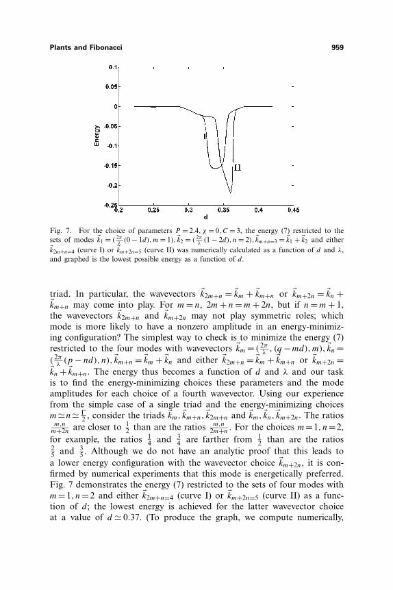
Fig. 7. For the choice of parameters P = 2.4, χ = 0,C = 3, the energy (7) restricted to thesets of modes �k1 = ( 2π

λ(0 − 1d),m = 1), �k2 = ( 2π

λ(1 − 2d), n = 2), �km+n=3 = �k1 + �k2 and either

�k2m+n=4 (curve I) or �km+2n=5 (curve II) was numerically calculated as a function of d and λ,and graphed is the lowest possible energy as a function of d.

triad. In particular, the wavevectors �k2m+n = �km + �km+n or �km+2n = �kn +�km+n may come into play. For m = n, 2m + n = m + 2n, but if n = m + 1,the wavevectors �k2m+n and �km+2n may not play symmetric roles; whichmode is more likely to have a nonzero amplitude in an energy-minimiz-ing configuration? The simplest way to check is to minimize the energy (7)restricted to the four modes with wavevectors �km = ( 2π

λ, (q −md),m), �kn =

( 2πλ

(p − nd), n), �km+n = �km + �kn and either �k2m+n = �km + �km+n or �km+2n =�kn + �km+n. The energy thus becomes a function of d and λ and our taskis to find the energy-minimizing choices these parameters and the modeamplitudes for each choice of a fourth wavevector. Using our experiencefrom the simple case of a single triad and the energy-minimizing choicesm�n� �

2 , consider the triads �km, �km+n, �k2m+n and �km, �kn, �km+2n. The ratiosm,n

m+2nare closer to 1

2 than are the ratios m,n2m+n

. For the choices m=1, n=2,for example, the ratios 1

4 and 34 are farther from 1

2 than are the ratios25 and 3

5 . Although we do not have an analytic proof that this leads toa lower energy configuration with the wavevector choice �km+2n, it is con-firmed by numerical experiments that this mode is energetically preferred.Fig. 7 demonstrates the energy (7) restricted to the sets of four modes withm=1, n=2 and either �k2m+n=4 (curve I) or �km+2n=5 (curve II) as a func-tion of d; the lowest energy is achieved for the latter wavevector choiceat a value of d � 0.37. (To produce the graph, we compute numerically,


for values of d and λ in a reasonable range, the energy-minimizing ampli-tudes and the value of the energy (7); the graph shows, for each value ofd, the lowest energy as a function of λ.) Note that this value of d is notexactly a value that makes any of the radial wavenumbers equal to 0; theenergy-minimizing choice of d is possibly irrational. Due to the indepen-dence of the energies (5) and (7), after scaling, on �, similar results holdfor larger values of m,n. In this case, the energy-minimizing amplitudesare such that am �am+2n <an �am+n; this produces parallelogram patternswith parastichy pair m,n; see Section 4.2.4.

4.2.4. Five Modes and Bias

Rather than separately testing the sets of overlapping triads �km, �kn,�km+n, �k2m+n and �km, �kn, �km+2n, we may allow for all five modes to competetogether. That is, we restrict the energy (7) to the five modes �km = ( 2π

λ, (q −

md),m), �kn = ( 2πλ

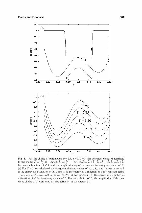
(p − nd), n), �km+n = �km + �kn, �k2m+n = �km + �km+n, �km+2n =�km + �km+n, and find the energy-minimizing choices of λ, d and modeamplitudes. In Fig. 8(a) we show (curve I) the graph of the energy as afunction of d for the choice m = 2, n = 3,� = m + n = 5. In this case, theenergy reaches a local minimum at the choices d �0.388 (for which choicethe amplitude A7 is small and A2 �A8 <A3 �A8) and d �0.412 (for whichchoice the amplitude A8 is small and A2 �A7 <A3 �A5). The latter choiceis slightly lower, so that a parastichy pair (5,7) minimizes the energy.

This calculation, however, disregards the effects of a previousconfiguration that has formed for a smaller value of � and moved radiallyoutward from the generative region. The effect of having, as a boundarycondition, a previously produced configuration is to add constant terms cj

to the amplitude equations so that the evolution of the amplitudes is givenby ∂tAj =− δE′

δA∗j, where E′ =cjAj +complex conjugate+E. Redoing the cal-

culation of Fig. 8(a), curve I, but adding constant terms c2 = c3 = c5, c7 =0=c8 to refect the chosen amplitudes for smaller �, the energy as a functionof d is as shown in Fig. 8(a), curve II. In this case, it is the amplitude con-figuration A2 � A8 < A3 � A5,A7 � 0 and d � 0.378 that are favored. Nowincreasing � in steps of 0.25 and using, as the constants cj , the energy-minimizing choices of amplitudes from the previous value of �, the choiced � 0.378 and the parastichy pair (5,8) remain preferred (Fig. 8(b)). Thus,the bias of a previous configuration helps to give preference to a parallelo-gram configuration with modes �km, �kn, �km+n, �km+2n.

In these five-mode experiments, one mode, either that with wavevector�k2m+n or �km+2n had a very small amplitude so that the energy-minimiz-ing configuration was close to the solution of a four-mode competition


Fig. 8. For the choice of parameters P = 2.4, χ = 0,C = 3, the averaged energy E restrictedto the modes �k2 = ( 2π

λ, (1 − 2d),2), �k3 = ( 2π

λ(1 − 3d),3), �k5 = �k2 + �k3, �k7 = �k2 + �k5, �k8 = �k3 + �k5

becomes a function of d, λ and the amplitudes An of the modes for any given value of �.(a) For � = 5 we calculated the energy-minimizing values of d, λ,An, and shown in curve Iis the energy as a function of d. Curve II is the energy as a function of d for constant termsc2 =c3 =c5 =0.5, c7 =c8 =0 in the energy E′. (b) For increasing �, the energy E is graphed asa function of d for increasing values of �. For each choice of �, the amplitudes of the pre-vious choice of � were used as bias terms cj in the energy E′.


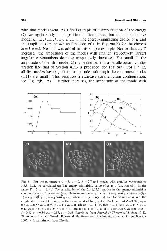
with that mode absent. As a final example of a simplification of the energy(7), we again study a competition of five modes, but this time the fivemodes �km, �kn, �km+n, �km+2n, �k2m+3n. The energy-minimizing choice of d andthe amplitudes are shown as functions of � in Fig. 9(a,b) for the choicesm=3, n=5. No bias was added in this simple example. Notice that, as �

increases, the amplitudes of the modes with smaller (respectively, larger)angular wavenumbers decrease (respectively, increase). For small �, theamplitude of the fifth mode (21) is negligible, and a parallelogram config-uration like that of Section 4.2.3 is produced; see Fig. 9(a). For � � 12,all five modes have significant amplitudes (although the outermost modes(3,21) are small). This produces a staircase parallelogram configuration;see Fig. 9(b). As � further increases, the amplitude of the mode with

Fig. 9. For the parameters C = 3, χ = 0, P = 2.7 and modes with angular wavenumbers3,5,8,13,21, we calculated (a) The energy-minimizing value of d as a function of � in therange � = 5, . . . ,18. (b) The amplitudes of the 3,5,8,13,21 modes in the energy-minimizingconfiguration as � increases. (c–e) Deformations w = a3 cos(�k3 · x) + a5 cos(�k5 · x) + a8 cos(�k8 ·x) + a13 cos(�k13 · x) + a21 cos(�k21 · �x), where �x = (s = ln(r), α) and for values of d and theamplitudes aj as determined by the experiment of (a,b), (c) at � = 8, so that d = 0.383, a3 =0.3, a5 = 0.52, a8 = 0.58, a13 = 0.3, a5 = 0, (d) at � = 11, so that d = 0.3815, a3 = 0.15, a5 =0.42, a8 = 0.53, a13 = 0.53, a21 = 0.15, and (e) at � = 14, so that d = 0.3815, a3 = 0.05, a +5 = 0.32, a8 = 0.54, a13 = 0.55, a21 = 0.38. Reprinted from Journal of Theoretical Biology, P. D.Shipman and A. C. Newell, Polygonal Planforms and Phyllotaxis, accepted for publication2005, with permission from Elsevier.


angular wavenumber 3 decreases to zero and the planform is again thatof parallelograms (Fig. 9(e)). Thus, a continuous transition from one par-allelogram planform to another is achieved through a continuous changein amplitudes and divergence angle.

4.2.5. Type I or II Transitions

We have, for simplicity, separately considered the cases of 3,4, or 5modes. To unite these ideas and give reasons for the choice of Type Ior II transitions, we suggest the following picture: Imagine that, for thechoice � =m+n, a sum of modes with amplitudes . . . , am−n, am, an, am+n,

am+2n, . . . is the energy-minimizing configuration. The configuration mayconsist of more modes, but the central modes are of largest amplitudeas the growth rate of a mode with radial wavenumber j decreases forj further from m + n. The relative size of the amplitudes is determinedby the parameters P and C. For small P , the linear growth rates, andtherefore the amplitudes, of the outer modes, will be small (negligible), sothat the configuration will be essentially that of a hexagon configuration(m,n,m + n). For large (but not too large) P , the outer amplitudes areno longer negligible, and the configuration is that of parallelograms orstaircase parallelograms. Similarly, a larger |C| yields a larger interactionbetween modes with angular wavenumbers (m−n,m,n) and thus increasesthe amplitude of the outer mode m − n even if it is relatively stronglylinearly damped.

Now suppose that the configuration . . . , am−n, am, an, am+n, am+2n, . . . ,formed for � � m + n, moves to the outer edge of the generative regionand acts as a bias on a newly forming configuration. If � does not change,then the new configuration will be as the old one. However, if � increases,say to m+n+1, then the linear growth rate of the m+2n-mode increases,as does the linear growth rate of the mode m+n+1.

I. The true energy-minimizing configuration involves the optimal triadwith radial wavenumbers (m,n + 1,m + n + 1) and a Type I transitionfrom the (m,n,m+n) configuration.

II. However, if the amplitude am+2n is large in the bias configuration, itcan grow continuously with � and give preference to a Type II transi-tion in which the amplitudes am+n and am+2n grow continuously as theamplitudes am−n, an decay.

Thus, Type II transitions are more likely when the outer members ofa sequence of amplitudes are larger. As a consequence, the theory predictsthat ridge-dominated planforms are more likely to undergo Type I transi-tions, whereas parallelogram planforms are more likely to undergo Type II


transitions. In agreement with the results of DC, the pattern produced byType II transitions are not necessarily absolute energy minimizers, but ratherlocal minimizers that are easily accessed from the previous configuration. Itis important therefore to not only find energy-minimizing configurations,but also to understand how they can be accessed from the previous state.

5. DISCUSSION

We now return to the question posed in the introduction, namely

(i) Can the same theory describe ridge-shaped and polygonal plan-forms?

(ii) In the case of polygonal planforms, what determines the posi-tions at which primordia (the polygons) form near the plant tipand therefore the phyllotactic pattern that develops?

(iii) What determines the type of phyllo that a primordium willdevelop into?

The first question is not addressed by DC, who assume that primor-dia of a given size and circular shape form on a parabaloid. Thus, in theDC model, the only difference in shape is the azimuthal elongation of pri-mordia as determined by the conicity parameter N . Our model allows forall the commonly seen simple planforms and also suggests that there isa connection between ridge or hexagon patterns and Type I transitionsand parallelogram patterns and Type II transitions–Type II transitions aremore likely when there is more than one triad with significantly largeamplitudes. Furthermore, the DC experiments suggest that the decussate(alternating 2-whorl) pattern can only be produced with azimuthally elon-gated primordia or conical apices and short-range interaction. Our modelalso produces ridge-dominated decussate patterns with radially elongatedprimordia as seen in some cacti.

To address the second question, which was the focus of the DCmodel, we first compare the parameters that were essential to both models.The main geometric parameter in the DC model is the ratio � = d0

Rof the

diameter of a newly formed primordium to the radius of the generativecircle. This parameter has almost an exact analog in our model, namelythe parameter � giving the ratio of the circumference of the central circleof the annular generative region to the natural wavelength; � is analogousto the inverse of �. Higher order phyllotactic patterns are produced as �

(respectively, �) is increased (respectively, decreased).The second geometric parameter concerns the curvature of the apex;

DC define a conicity parameter N which determines the curvature ofthe apex. Our curvature parameter C is different in that it is only


relevant in the generative region. In order to produce hexagon patternsin which the centers of the hexagons are the maxima (rather than theminima) of the deformation, our model requires that the geometry of thegenerative region be that of an inverted circle or hyperbolic, as depicted inFig. 4(b,c). Our parameter C is also analogous to the DC stiffness param-eter α. While α measures the degree that old primordia influences newones (and thus a sort of interaction between primordia), in our modelC measures the degree of interaction between triads of modes in thegenerative region. The essential difference between our two models is thatprimordia interact in the DC paradigm, whereas the elementary compo-nents that interact in our model are periodic modes.

DC propose, based on their paradigm, that the essential componentsfor a mechanical model are that it (i) defines a finite area for new pri-mordia, and (ii) allows for “repulsion” of some sort. Our mechanism doesdefine a finite area A = 2π λ

gR� which is essential for the results, but,

instead of a repulsion between primordia, the essential points are that (1)the critical mode has wavevector (0,�), (2) the interaction coefficient τ issensitive to d and dependent on λ, (3) bias, which is relevant if there isone than one triad present, is essential to producing Type II transitionsand the Fibonacci sequence. However, even if there is bias, if the defor-mation is dominated by one mode, Type I transitions are preferred overType II transitions.

Regarding the difference between Type I and II transitions, DC pro-pose that Type I transitions are preferred unless a quick change in �

allows a continuous Type II transition to take hold. In our model, theType I transition is also energetically preferred unless the deformationconsists of more than one overlapping triad and a bias allows a modeof small amplitude to continuously grow in size with �. A consequenceof this is the prediction that ridge-dominated planforms are more likelyto undergo Type I transitions, whereas parallelogram planforms are morelikely to undergo Type II transitions. While this conclusion conforms withour observations of cacti, there are no published data for a wide varietyof plants. Green et al.(11) proposed that the difference between the forma-tion of whorls and spirals (and thus, presumably between Type I and IItransitions) is based on the width of the annular generative region. Thisis not included in our model, as we have approximated the Laplacian bythe Euclidean Laplacian ∂2

r + 1�2 ∂2

α; a further modification of our modelcould test the idea of Green.

The DC model produces periodic (in d) transients during transi-tions between a (1,2,3) spiral and a decussate (2,2,4) phyllotactic pattern.Our model as presented here produces a sudden transition in which one


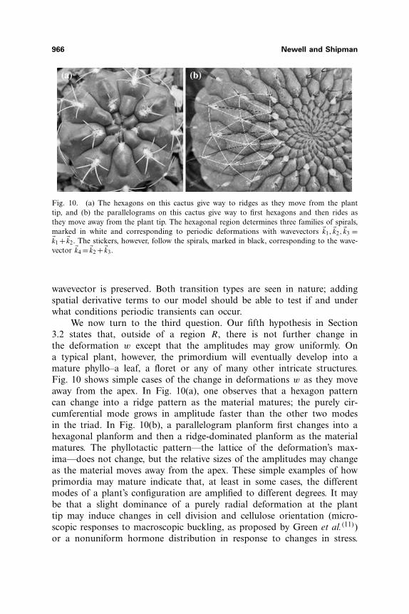
Fig. 10. (a) The hexagons on this cactus give way to ridges as they move from the planttip, and (b) the parallelograms on this cactus give way to first hexagons and then rides asthey move away from the plant tip. The hexagonal region determines three families of spirals,marked in white and corresponding to periodic deformations with wavevectors �k1, �k2, �k3 =�k1 + �k2. The stickers, however, follow the spirals, marked in black, corresponding to the wave-vector �k4 = �k2 + �k3.

wavevector is preserved. Both transition types are seen in nature; addingspatial derivative terms to our model should be able to test if and underwhat conditions periodic transients can occur.

We now turn to the third question. Our fifth hypothesis in Section3.2 states that, outside of a region R, there is not further change inthe deformation w except that the amplitudes may grow uniformly. Ona typical plant, however, the primordium will eventually develop into amature phyllo–a leaf, a floret or any of many other intricate structures.Fig. 10 shows simple cases of the change in deformations w as they moveaway from the apex. In Fig. 10(a), one observes that a hexagon patterncan change into a ridge pattern as the material matures; the purely cir-cumferential mode grows in amplitude faster than the other two modesin the triad. In Fig. 10(b), a parallelogram planform first changes into ahexagonal planform and then a ridge-dominated planform as the materialmatures. The phyllotactic pattern—the lattice of the deformation’s max-ima—does not change, but the relative sizes of the amplitudes may changeas the material moves away from the apex. These simple examples of howprimordia may mature indicate that, at least in some cases, the differentmodes of a plant’s configuration are amplified to different degrees. It maybe that a slight dominance of a purely radial deformation at the planttip may induce changes in cell division and cellulose orientation (micro-scopic responses to macroscopic buckling, as proposed by Green et al.(11))or a nonuniform hormone distribution in response to changes in stress.


Furthermore, note in Fig. 10(b) that, even as one spiral mode (marked inblack) decays in amplitude, the stickers that form are aligned along thedirection of this decaying mode. Thus, although the processes that lead tointricate phylla such as leaves or florets are much more involved than thesesimple examples, the presence of elementary modes suggest simple ways inwhich to study the feedback mechanisms between stresses, chemistry andgrowth.

In contrast to the suggestion made above that mechanical bucklinginitiates primordia and is followed by changes in plant hormone concen-trations, a growing biological community believes that the initiation of pri-mordia is also chemical. In particular, recent work has focused on thegrowth hormone auxin and the role of the PIN1 protein in auxin trans-port; see Reinhardt,(14) for a review. Models based on these ideas are ableto reproduce spiral or whorl patterns, but, like the DC model, do notexplain ridge patterns.

In,(16) we further discuss predictions of the mechanical model andsuggest experiments and observations to test the theory.

REFERENCES

1. T. M. Atanackovic and A. Guran, Theory of Elasticity for Scientists and Engineers (Birk-haeuser, 2000).

2. S. Douady and Y. Couder, phyllotaxis as a physical self-organizing growth process, Phys.Rev. Lett. 68:2098–2101 (1992).

3. S. Douady and Y. Couder, Phyllotaxis as a dynamical self-Organizing process, part i: Thespiral modes resulting from time-periodic iterations, J. Theor. Biol. 178:255–274 (1996).

4. S. Douady and Y. Couder, Phyllotaxis as a dynamical self-organizing process, part ii: Thespontaneous formation of a periodicity and the coexistance of spiral and whorled pat-terns, J. Theor. Biol. 178:275–294 (1996).

5. J. Dumais and C. R. Steele, New Evidence for the role of mechanical forces in the shootapical meristem, J. Plant Growth Reg. 19:7–18 (2000).

6. J. Farber, H. C. Lichtenberger, A. Reiterer, S. Stanzl-Tschegg, and P. Fratzl, Cellu-lose microfibril angles in a spruce branch and mechanical implications, J. Mat. Sci.36:5087–5092 (2001).

7. A. J. Fleming, S. McQueen-Mason, T. Mandel, and C. Kuhlemeier, Induction of LeafPrimordia by the Cell Wall Protein Expansin, Science 276:1415–1418 (1997).

8. P. L. Gould, Analysis of Plates and Shells, (Prentice Hall, 1999).9. P. Green, Expression of Pattern in Plants: Combining Molecular and Calculus-Based

Biophysical Paradigms, Am. J. Bot. 86:1059–1076 (1999).10. P. B. Green, Expression of form and pattern in plants. a role for biophysical fields, Cell.

Dev. Biol. 7:903–911 (1996).11. P. B. Green, C. S. Steele, and S. C. Rennich, How plants produce patterns. A review and

a proposal that undulating field behavior is the mechanism, in Symmetry in Plants, RogerV. Jean and Denis Barabe, eds. (World Scientific, 1998).

12. L. H. Hernandez and P. B. Green, Transductions for the Expression of StructuralPattern: Analysis in Sunflower, Plant Cell 5:1725-1738 (1993).


13. W. Hofmeister, Allgemeine Morphologie der Gewachse, Handbuch der PhysiologischenBotanik, (Engelmann, 1868).

14. D. Reinhardt, A new chapter in an old tale about beauty and magic numbers, CurrentOpinion in Plant Biology 8:1–7 (2005).

15. P. D. Shipman and A. C. Newell, Phyllotactic patterns on plants, Phys. Rev. Lett.92:168102 (2004).

16. P. D. Shipman and A. C. Newell, polygonal planforms and phyllotaxis on plants,J. Theo. Biol. 236:154–197 (2005).

17. M. Snow and R. Snow, Minimum areas and leaf determination, Proc. Roy. Soc. 545–566(1952).

18. C. R. Steele, Shell stability related to pattern formation in plants, J. Appl. Mech. 67:237–247 (2000).

19. H. Yamamoto, generation mechanism of growth stresses in wood cell walls, Wood Sci.and Technol. 32:171–182 (1998).

plants and fibonacci - university of...

Documents