local normal forms for geodesically equivalent pseudo...
TRANSCRIPT

Local normal forms for geodesically equivalent
pseudo-Riemannian metrics
Alexey V. Bolsinov∗† & Vladimir S. Matveev‡§
Abstract
Two pseudo-Riemannian metrics g and g are geodesically equivalent, if they share thesame (unparameterized) geodesics. We give a complete local description of such metricswhich solves the natural generalisation of Beltrami problem for pseudo-Riemannian metrics.
1 Introduction
1.1 Definition and history
Two pseudo-Riemannian metrics g and g on one manifold Mn are geodesically equivalent, if everyg-geodesic, after an appropriate reparameterisation, is a g-geodesic. Theory of geodesically equiv-alent metrics has a long and rich history, the first examples were constructed already by Lagrange[23], and many important results about geodesically equivalent metrics were obtained by clas-sics such as Beltrami [3, 4, 5], Levi-Civita [25], Painleve [35], Lie [26], Liouville [27], Fubini [18],Eisenhart [16, 17], Weyl [43], Thomas und Veblen [40, 41, 42]. In the 50th-90th, the theory ofgeodesically equivalent metrics was one of the main research areas of the Soviet and Japanesedifferential geometry schools, see the surveys [2, 34]. In the recent time, the theory of geodesicallyequivalent metrics has a revival because of new mathematical methods that came here, in par-ticular, from the theory of integrable systems [28] and from parabolic Cartan geometry [12, 15].Using these methods led, in the last ten years, to the solution of many problems explicitly statedby classics including Sophus Lie problems [11, 33], Lichnerowicz conjecture [31], and Weyl-Ehlersproblems [20, 32].
In the present paper we solve the natural generalization of one more problem explicitly stated bya classic to the pseudo-Riemannian metrics, namely
Beltrami Problem1. Describe all pairs of geodesically equivalent metrics.
From the context it is clear that Beltrami actually considered this problem locally and in a neigh-borhood of almost every point, so do we. From the contex it is also clear that Beltrami thoughtabout two dimensional Riemannian surfaces; in our answer we do not have this restriction: thedimension of the manifold, and the signatures of the metrics are arbitrary.
Special cases of the Beltrami problem were known before. The two-dimensional Riemannian casewas solved already by Dini [14]: he has shown that two Riemannian geodesically equivalent metricson a surface in a neighborhood of almost every point are given in a certain coordinate system by
∗School of Mathematics, Loughborough University, LE11 3TU, UK [email protected]†Partially supported by Ministry of Education and Science of the Russian Federation (14.B37.21.1935)‡Institute of Mathematics, 07737, Jena, Germany [email protected]§Partially supported by DFG (GK 1523) and DAAD (Programm Ostpartnerschaft)1Italian original from [3]: La seconda . . . generalizzazione . . . del nostro problema, vale a dire: riportare i
punti di una superficie sopra un’altra superficie in modo che alle linee geodetiche della prima corrispondano linee
geodetiche della seconda
1

the following formulas
g = (Y (y) − X(x))(dx2 + dy2) and
(1
X(x)−
1
Y (y)
)(dx2
X(x)+
dy2
Y (y)
)
. (1)
Here X and Y are functions of the indicated variables. For every (smooth) functions X,Y suchthat the formulas (1) correspond to Riemannian metrics (i.e., 0 < X(x) < Y (y) for all (x, y)) themetrics g and g are geodesically equivalent.
For an arbitrary dimension, the Beltrami problem in the Riemannian case was solved by Levi-Civita [25]. We will recall the Levi-Civita’s 3-dimensional analog of the formulas (1) below, inExample 2.
The methods of Levi-Civita and Dini can not be directly generalized to the pseudo-Riemanniancase. Levi-Civita and Dini consider the tensor G defined by the condition g(G., .) = g(., .). Levi-Civita has shown, that the eigenspaces of this tensor are simultaneously integrable which impliesthat (in a neighborhood of almost every point) there exists a local coordinate system
(x1, ..., xn) = (x11, ..., x
m11 , ..., x1
k, ..., xmk
k )
such that in these coordinates the matrix of g is blockdiagonal with k blocks of dimensionm1,m2, ...,mk and the matrix of G is diagonal diag(ρ1, ..., ρ1
︸ ︷︷ ︸
m1
, ..., ρk, ..., ρk︸ ︷︷ ︸
mk
). In the two-dimensional
Riemannian case considered by Dini, the existence of such coordinate system is obvious. Now, inthis coordinate system, the partial differential equations on the entries of g and on ρi expressingthe geodesic equivalence condition for g and g = g(G., .) are relatively easy (though they are stillcoupled) and, after some nontrivial work, can be solved.
The methods of Levi-Civita also work in the pseudo-Riemannian case under the additional as-sumption that G is diagonalizable. Unfortunately, in the pseudo-Riemannian case the tensor Gmay have complex eigenvalues and Jordan blocks. From the point of view of partial differentialequation, the case of many Jordan blocks poses the main difficulties: unlike the case when G isdiagonalizable, there is no ‘best’ coordinate system, and the equation corresponding to the entriesof the metrics coming from different blocks are coupled in a very nasty manner.
This difficulty was overcome in [9]. In §1.2 we recall the main result of [9] and explain that thedescription of geodesically equivalent metrics g and g in a neighborhood of almost every point canbe reduced to the case when the tensor G has one real eigenvalue only, or two complex-conjugatedeigenvalues. The biggest part of our paper is devoted to the local description of geodesicallyequivalent metrics under this assumption.
Special cases of the local description of geodesically equivalent pseudo-Riemannian metrics wereknown before. The 2-dimensional case was described essentially by Darboux [13, §§593, 594], seealso [7, 8]. Three dimensional case was solved by Petrov [36], it is one of the results Petrov obtainedin 1972 the Lenin prize for, the most important scientific award of the Soviet Union. According to[2], under the additional assumptions that the metrics g and g have Lorentz signature, the Beltramiproblem was solved by Golikov [19] in dimension 4, and by Kruchkovich [22] in all dimensions;unfortunately, we were not able to find and to verify these references.
It was generally believed that the Beltrami problem was solved in full generality in [1]. Unfortu-nately, this result of Aminova seems to be wrong. More precisely, in view of [1, Theorem 1.1] andthe formulas [1, (1.17),(1.18)] for k = 1, n = 4 and all ε’s equal to +1, the following two metricsg and g given by the matrices (where ω is an arbitrary function of the variable x4)
0 0 0 3x3 + 3ω (x4)
0 0 1 2x2
0 1 0 x1
3x3 + 3ω (x4) 2x2 x1 4x1x2
,
2

26666666666666666640 0 0 3
x3+ω(x4)
x45
0 0 2 x4−5 −3 x3−3 ω(x4)+2 x2x4
x46
0 2 x4−5
−x4−6 3 x3+3 ω(x4)−2 x2x4+x1x4
2
x47
3x3+ω(x4)
x45
−3 x3−3 ω(x4)+2 x2x4x4
63 x3+3 ω(x4)−2 x2x4+x1x4
2
x47
(−3 x3−3 ω(x4)+2 x2x4)�2 x1x4
2+3 x3+3 ω(x4)−2 x2x4
�x4
8
3777777777777777775should be geodesically equivalent, though they are not (which can be checked by direct calcula-tions).
1.2 Splitting and gluing construction: why it is sufficient to assume that
G has one real eigenvalue or two complex-conjugated eigenvalues.
Given two metrics g and g on the same manifold, instead of considering the (1, 1)-tensor Gij =
gikgkj , we consider the (1, 1)−tensor L = L(g, g) defined by
Lij :=
(det(g)
det(g)
) 1n+1
gikgkj , (2)
where gik is the contravariant inverse of gik. The tensors G and L are related by a simple relation
L = det(G)1
n+1 G−1, G = 1det(L)L
−1, (3)
so in particular they have the same structure of Jordan blocks (though the eigenvalues are, ingeneral, different). Since the metric g can be uniquely reconstructed from g and L, namely:
g(· , ·) = 1det(L)g(L−1· , ·) (4)
the condition that g is geodesically equivalent to g can be written as a PDE-system on the compo-nents of L. From the point of view of partial differential equations, the tensor L is more convenientthan G: the corresponding system of partial differential equations on L turns out to be linear. Inthe index-free form, it can be written as the condition (where “∗” means g−adjoint)
∇uL =1
2(u ⊗ dtrL + (u ⊗ dtrL)∗), (5)
which should be fulfilled at every point and for every vector field u.
In tensor notation, the condition (5) reads
Lij,k = λ,igjk + λ,jgik, (6)
where Lij := Lkj gki and λ := 1
2Lii = 1
2 tr (L). The tensor Lij defined in (2) is essentially the same
as the tensor introduced by Sinjukov (see equations (32, 34) on the page 134 of the book [37], andalso Theorem 4 on page 135); the equation (6) is also due to him, see also [6, Theorem 2].
Remark 1. If n is even, the tensor L is always well defined. If n is odd, the ratio det(g)/det(g)may be negative, and then formula (2) has no sense. There is the following way to avoid this(rather, formal) difficulty: we can replace g by −g and make the ratio det(g)/det(g) positive andL well defined. Moreover, since the equations (5) are linear, we can assume that L is close to 1
in the neighborhood we are working in, implying that g and g have the same signatures, and theproblem with the sign does not appear at all.
We say that the (1,1)-tensor L is compatible with g, if it is g-selfadjoint, nondedenerate at everypoint, and satisfies (5) at any point and for all tangent vectors u. As we explain above, L iscompatible with g if and only if g(., .) = 1
det(L)g(L−1., .) is a pseudo-Riemannian metric geodesically
equivalent to g.
3

Let us now recall the gluing construction from [9]. The construction, and also the splitting con-struction to be recalled below, is due to [9]; in the Riemannian case it appeared slightly earlier,see [29, §4], [31, Lemma 2] and [30, §§2.2, 2.3].
Consider two pseudo-Riemannian manifolds (M1, h1) and (M2, h2). Assume that L1 on M1 iscompatible with h1, and that L2 on M2 is compatible with h2. Assume in addition that L1 andL2 have no common eigenvalues in the sense that for any two points x ∈ M1, y ∈ M2 we have
SpectrumL1(x) ∩ SpectrumL2(y) = ∅. (7)
Then one can naturally and canonically construct a pseudo-Riemannian metric g and a tensor Lcompatible with g on the direct product M = M1 ×M2. The new metrics g differs from the directproduct metric h1 + h2 on M1 × M2 and is given by the following formula involving L1 and L2:we denote by χi, i = 1, 2, the characteristic polynomial of Li: χi = det(t ·1i −Li) (where 1i is theidentical operator 1i : TMi → TMi). We treat the (1, 1)−tensors Li as linear operators acting onTMi. For a polynomial f(t) = a0 + a1t + a2t
2 + · · · + amtm and an (1, 1)-tensor A we put f(A)to be the (1, 1)-tensor
f(A) = a0 · 1 + a1A + a2A ◦ A + · · · + am A ◦ · · · ◦ A︸ ︷︷ ︸
m times
.
If no eigenvalue of A is a root of f , f(A) is nondegenerate; if A is g-selfadjoint, f(A) is g-selfadjointas well.
For two tangent vectors u = ( u1︸︷︷︸
∈TM1
, u2︸︷︷︸
∈TM2
) , v = ( v1︸︷︷︸
∈TM1
, v2︸︷︷︸
∈TM2
) ∈ TM we put
g(u, v) = h1 (χ2(L1)(u1), v1) + h2 (χ1(L2)(u2), v2) , (8)
L(v) = (L1(v1), L2(v2)) . (9)
We see that the (1, 1)−tensor L is the direct sum of L1 and L2 in the natural sense.
It might be convenient to understand the formulas (8, 9) in the matrix notation: we considerthe coordinate system (x1, ..., xr, yr+1, ..., yn) on M such that x’s are coordinates on M1 and y’sare coordinates on M2. Then, in this coordinate system, the matrices of g and L have the blockdiagonal form
g =
(h1χ2(L1) 0
0 h2χ1(L2)
)
, L =
(L1 00 L2
)
. (10)
If (7) is fulfilled, then g is a pseudo-Riemannian metric (i.e., symmetric and nondegenerate) andL is nondegenerate and g-selfadjoint.
Theorem 1 (Gluing Lemma from [9]). If L1 is compatible with h1 on M1 and L2 is compatiblewith h2 on M2, and if the condition (7) is fulfilled, then L given by (9) is compatible with g givenby (8).
Example 1 (Gluing construction and Dini’s Theorem). As the manifolds M1,M2 we take twointervals I1 with the coordinate x and I2 with the coordinate y. Next, take the metrics h1 = dx2 onI1 and h2 = −dy2 on I2. Consider the (1,1)-tensors L1 = X(x)dx⊗ ∂
∂xon I1 and L2 = Y (y)dy⊗ ∂
∂y
on I2. We assume that 0 < X(x) < Y (y) for all x ∈ I1 and y ∈ I2. The tensors L1 and L2 arecompatible with h1 resp. h2 (which can be checked by direct calculation and which is trivialin view of the obvious fact that in dimension 1 all metrics are geodesically equivalent). Then,χ1 = (t − X(x)), χ2 = (t − Y (y)), so the formulas (10) read
g =
(Y (y) − X(x)
Y (y) − X(x)
)
, L =
(X(x)
Y (y)
)
.
4

Now, combining this with (4), we obtain that this g is geodesically equivalent to the metric
g =Y (y) − X(x)
X(x)Y (y)
(1
X(x)1
Y (y)
)
=
(1
X(x)−
1
Y (y)
)( 1X(x)
1Y (y)
)
.
Comparing the above formulas with (1), we see that gluing construction applied to two intervalsproves Dini’s local description of geodesically equivalent metrics in one direction.
One can iterate this construction: having three pseudo-Riemannian manifolds (M1, h1), (M2, h2),(M3, h3) carrying gi-compatible (1, 1)-tensors Li such that the condition (7) is mutually fulfilled,one can glue M1 and M2 and then glue the result with M3. Actually the gluing constructionis associative. Indeed, one obtains the same metric g and the same g-compatible (1, 1)-tensor Lon M1 + M2 + M3 if one first glues (M1, h1, L1) and (M2, h2, L2) and then glues the result with(M3, h3, L3), or if one first glues (M2, h2L2) and (M3, h3, L3) and then glues (M1, h1, L1) with theresult:
((M1, h1, L1)
glue
+ (M2, h2, L2)) glue
+ (M3, h3, L3) = (M1, h1, L1)glue
+((M2, h2, L2)
glue
+ (M3, h3, L3)).
The gluing construction is commutative as well:
(M1, h1, L1)glue
+ (M2, h2, L2)iso= (M2, h2, L2)
glue
+ (M1, h1, L1),
where “iso=” means the existence of a diffeomorphism that preserves the metric and L. Actually,
this diffeomorphism is given by the natural formula
M1 × M2 ∋ ( x︸︷︷︸
∈M1
, y︸︷︷︸
∈M2
) 7→ ( y︸︷︷︸
∈M2
, x︸︷︷︸
∈M1
) ∈ M2 × M1.
In the case we “glue” k manifolds (Mi, hi) (i = 1, . . . , k) such that each manifold is equipped withhi-compatible Li, we obtain a metric g on M = M1 × · · · × Mk and g-compatible L on M suchthat in the matrix notation in the natural coordinate system they have the form
g =
h1χ2(L1) · · ·χk(L1)h2χ1(L2)χ3(L2) · · ·χk(L2)
. . .
hkχ1(Lk) · · ·χk−1(Lk)
, (11)
L =
L1
L2
. . .
Lk
. (12)
Example 2 (Gluing construction and Levi-Civita’s Theorem in dim 3). We now take three intervalsI1, I2, I3 with the coordinates x, resp. y, z, the metrics h1 = dx2, h2 = −dy2, h3 = dz3, and thehi-compatible (1, 1)-tensors L1 = X(x)dx ⊗ ∂
∂x, L2 = Y (y)dy ⊗ ∂
∂y, and L3 = Z(z)dz ⊗ ∂
∂z. We
again assume that the spectra of Li are mutually disjunkt at every point, without loss of generalitywe assume
0 < X(x) < Y (y) < Z(z) ∀x ∈ I1, ∀y ∈ I2 ∀z ∈ I3.
Applying the gluing construction two times, we obtain that, on M3 = I1×I2×I3 with the naturalcoordinate system, the (1, 1)-tensor L below is compatible with the metric g below.
g =
(Y (y) − X(x))(Z(z) − X(x))(Y (y) − X(x))(Z(z) − Y (y))
(Z(z) − Y (y))(Z(z) − X(x))
,
5

L =
X(x)Y (y)
Z(z)
.
Combining this with (4), we obtain a special case of Levi-Civita’s local description of geodesicallyequivalent metrics in dimension 3 (when the tensor G has three different eigenvalues).
The splitting construction is the inverse operation. We will describe its local version only since itis sufficient for our goals.
Suppose g is a pseudo-Riemannian metric on Mn and L is compatible with g. We consider anarbitrary point p ∈ M .
We take a point p of the manifold such that in the neighborhood U(p) of this point the eigenvaluesof L do not bifurcate (i.e., the number of different eigenvalues is constant in the neighborhood).Then, the eigenvalues are smooth possibly complex-values functions: we denote them by
λ1, λ1, ... , λr, λr : U(p) → C, λr+1, ... , λk : U(p) → R.
We assume that for i ≤ r the eigenvalue λi is complex-conjugate to λi. We think that theeigenvalue λi has algebraic multiplicity mi, 2m1 + · · · 2mr + mr+1 + · · ·mk = n.
Next, let us consider the polynomial functions χi : R × U(p) → R:
χi = (t − λi)mi(t − λi)
mi for i = 1, ..., r and χi = (t − λi)mi for i = r + 1, ..., k,
and the polynomial function χ := χ1 + ... + χk, where χi = χχi
and χ = det(t · 1 − L) is the
characteristic polynomial of L. It is easy to see that the (1,1)-tensor χ(L) is g-selfadjoint andnondegenerate. Then we can introduce a new pseudo-Riemannian metric h on U(p) by
h(u, v) := g(χ(L)−1u, v), u, v ∈ TqM, q ∈ U(p). (13)
Theorem 2 (Follows from the splitting Lemma, see §2.1 of [9]). In a neighborhood of p thereexists a coordinate system
(x1, ... , xk) =(x1
1, ... , x2m11 , · · · , x1
r, ... , x2mrr , x1
r+1, ... , xmr+1
r+1 , · · · , x1k1, ... , x
mk
k
)
such that in this coordinate system the matrices of h and of L are given by
h =
h1
h2
. . .
hk
, L =
L1
L2
. . .
Lk
. (14)
Moreover,
• the entries of the blocks hi and Li depend on the coordinates xi only;
• for i = 1, ... , r the eigenvalues of Li are λi and λi, and for i = r+1, ... , k the only eigenvalueof Li is λi;
• Li is compatible with hi for every i = 1, ... , k (i.e., for every i = 1, ..., k the restriction ofL to the coordinate plaque of the coordinates xi, which in the coordinates xi is given by thematrix Li, is compatible with the restriction of h to this plaque, which in coordinates xi isgiven by the matrix hi).
Example 3 (Splitting construction and Dini’s Theorem). We consider a two dimensional manifoldM2 and geodesically equivalent Riemannian metrics g and g on it. We take a point where themetrics are not proportional; then, L(g, g) has two (real) eigenvalues in every point of a small
6

neighborhood U(p). Then, in the notation of Theorem 2, k = 2, r = 0, and m1 = m2 = 1. Then,χ1 = t − λ1, χ2 = t − λ2 and χ = (t − λ2) + (t − λ1). Then, there exists a coordinate system x, ysuch that h, L, and χ(L) are given by the matrices
h =
(X(x)
Y (y)
)
, L =
(X(x)
Y (y)
)
, χ(L) =
(Y (y) − X(x)
X(x) − Y (y)
)
.
Combining this with (4), (13), we see that the metrics g and g are given by
g = (Y (y) − X(x))(X(x)dx2 + Y (y)dy2) and
(1
X(x)−
1
Y (y)
)(
X(x)dx2
X(x)+
Y (y)dy2
Y (y)
)
.
By a coordinate change of the form xnew = xnew(x), ynew = ynew(x) one can ‘hide’ X in dx2 andY in dy2 and obtain the metrics of the form (1).
We call a point p ∈ M regular, if in some neighborhood U(p) of p the Jordan type of L is constant(that is, the number of eigenvalues and Jordan blocks is the same at all points x ∈ U(p); the sizesof Jordan blocks are assumed to be fixed too, whereas the eigenvalues can, of course, depend onthe point). It is easy to see that almost every point of M is regular, that is, the set of regularpoints is open and everywhere dense on the manifold.
Now, applying the Splitting Lemma in the neighborhood of a regular point, we obtain the metricshi on 2mi- or mi dimensional discs, and (1,1)-tensors Li compatible with hi. Moreover, each Li
has one real or two complex eigenvalues, and the Jordan type of Li is the same at all points.
If we describe all possible hi and Li satisfying these conditions, we will describe then all possiblegeodesically equivalent metrics g and g near regular points: all possible g and g-compatible L canbe obtained by the gluing construction (which is given by explicit formulas (11,12), and the metricg is constructed from g and L by the formula g(· , ·) = 1
det(L)g(L−1· , ·).
Finally, in order to describe the metric and L in the neighborhood of almost any point, it issufficient to describe the metrics hi and the hi-compatible Li such that Li has one real eigenvalue,or two complex-conjugate eigenvalues, and the type of the Jordan block is the same in the wholeneighborhood. We will formulate the result in § 1.3, see Theorems 3, 4, 5 there, the proof of thesetheorems will be given in Sections 2, 3 and 4.
1.3 Canonical forms for basic blocks
Throughout this section we assume that p ∈ M is a regular point, i.e. the Jordan type of L remainsunchanged in some neighborhood of p. Our goal is to find local normal forms for compatible Land g nearby p.
According to the previous section (Theorem 2), it is sufficient to describe the structure of com-patible pairs (g, L) in the case when L either has a single real eigenvalue λ, or has a pair ofcomplex eigenvalues λ, λ. However even in these cases, the situation depends essentially of thealgebraic structure of L, more precisely of the geometric multiplicity of λ, i.e., the number of lin-early independent eigenvectors. There are three essentially different possibilities: 1) the geometricmultiplicity of λ is at least two, 2) L is conjugate to a real Jordan block (i.e. L has a single realeigenvalue λ of geometric multiplicity one) and 3) L is conjugate to a pair of complex conjugateJordan blocks (i.e., L has a pair of complex conjugate eigenvalues each of geometric multiplicityone). These cases are described by Theorems 3, 4 and 5 below.
We start with the case of multiplicity ≥ 2. This situation turns out to be very special. Namely,the following statement holds.
Theorem 3. Let g and L be compatible, i.e., satisfy (5) and in a neighborhood U of a point p ∈ Mthe operator L has either a unique real eigenvalue λ = λ(x) or a unique pair of complex conjugate
7

eigenvalues λ(x), λ(x). Suppose that the geometric multiplicity of λ is at least two at each pointx ∈ U . Then the function λ(x) is constant and L is covariantly constant in U , i.e., ∇L = 0. Inparticular the metrics g and g given by (4) are affinely equivalent.
Thus, in the case of geometric multiplicity ≥ 2, our problem is reduced to another rather non-trivial problem of local classification of pairs g, L satisfying ∇L = 0, which has been recentlycompletely solved by Charles Boubel and we refer to his work [10] for further details.
We now give the answer for L being conjugate to a single real Jordan block, in other words weassume that the eigenvalue λ is real and L possesses a unique (up to proportionality) eigenvector.
Theorem 4. Let g and L be compatible, i.e., satisfy (5), and L be conjugate to a single Jordanblock with a real eigenvalue λ. Then there exists a local coordinate system x1, . . . , xn such that
g =
an−1
1 an−2
. .. ...
1 a1
an−1 an−2 . . . a2
∑n−2i=1 aian−i−1
and
L =
λ(xn) 1 a1
λ(xn) 1 a2
. . .
λ(xn) an−1
λ(xn)
wherea1 = λ′
xnx1,
a2 = 2λ′xn
x2,
. . .
an−2 = (n − 2)λ′xn
xn−2,
an−1 = 1 + (n − 1)λ′xn
xn−1.
and λ = λ(xn) is an arbitrary function. Conversely, if λ = λ(xn) is an arbitrary smooth functionsuch that λ(xn) 6= 0 for all xn, then g and L given by the above formulas are compatible (in thedomain where g is non-degenerate, i.e. 1 + (n − 1)λ′
xnxn−1 6= 0).
Remark 2. Equivalently, one can write g as the symmetric 2-form
n∑
k=1
(dxk + (k − 1)λ′xn
xk−1dxn)(dxn−k+1 + (n − k)λ′xn
xn−kdxn).
The (1,1)-tensor L, in this notation, takes the following form:
L = λ(xn) · 1 +
n−1∑
k=1
∂xk⊗ dxk+1 + λ′
xn
(n−1∑
k=1
kxk∂xk
)
⊗ dxn.
Remark 3. In the case when λ′xn
6= 0 at the point p, we can simplify these formulas even furthertaking λ(xn) as a new coordinate. After the change xnew
n = λ(xn) we obtain the following normalforms for L and g (we keep the “old” notation xn for the “new” coordinate).
Let g and L be compatible, i.e., satisfy (5), and L be conjugate to a Jordan block with a realeigenvalue λ. If dλ(p) 6= 0, then in a neighborhood of p ∈ M there exists a local coordinate system
8

x1, . . . , xn such that λ = xn and
g =
h(xn)+(n−1)xn−1
1 (n − 2)xn−2
. .. ...
1 x1
h(xn)+(n−1)xn−1 . . . . . . x1
∑
(15)
and
L =
xn 1 x1
xn 1 2x2
. . ....
xn h(xn)+(n−1)xn−1
xn
(16)
where∑
=∑n−2
i=1 i(n − i + 1)xixn−i−1 and h(xn) is an arbitrary function such that h(0) 6= 0.Conversely, g and L given by these formulas are compatible for every h(xn) (in the domain whereh(xn) + (n − 1)xn−1 6= 0).
Remark 4. it follows immediately from the proof (see Section 3) that the canonical coordinatesystem (and hence canonical forms) for g and L from Theorem 4 is uniquely defined (up to a finitegroup) if we fix the position of the initial point p ∈ M by saying that p is the origin of the canonicalcoordinate system. If we do not fix p, i.e., move the origin to another point p′ ∈ U(p), then thefunction h(xn) playing the role of the parameter for canonical forms (15) and (16) changes. It isnot difficult to check that the transformation that preserves the structure of (15) and (16) has thefollowing form:
xn = xn,xn−1 = xn−1 + p(xn),xn−2 = xn−2 −
1n−2p′(xn),
. . .xn−k = xn−k + (−1)k−1 1
(n−2)(n−3)...(n−k)p(k−1)(xn),
. . .x1 = x1 + (−1)n−2 1
(n−2)!p(n−2)(xn).
Here p(xn) is an arbitrary polynomial of degree n − 2 and p(k) denotes its kth derivative. Thefunction h(xn) after this change of variables takes the form h(xn) − (n − 1)p(xn). Thus we seethat the function h, the parameter of our canonical form, is defined modulo a polynomial of degreen − 2.
The next case is a complex Jordan block, i.e. we assume that the only eigenvalues of L are a pairof complex conjugate numbers λ and λ for each of which there is a single (up to proportionality)eigenvector over C. Equivalently, this means that the corank of the real operator (L−λ·1)(L−λ·1)is two. In this case, the normal form for g and L can be described in the following way.
Theorem 5. Let g and L be compatible, i.e., satisfy (5), and L be conjugate to a complex Jordanblock with complex conjugate eigenvalues λ and λ (Im λ 6= 0). Then there exists a complex structureJ and a local complex coordinate system (z1, . . . , zn) such that
1. the eigenvalue λ is a holomorphic function of zn,
2. L is a complex linear operator on (TP M,J) given in this coordinate system by the matrix:
LC =
λ(zn) 1 a1
λ(zn) 1 a2
. . .
λ(zn) an−1
λ(zn)
9

3. the metric g is the real part of the complex bilinear form on (TP M,J) given in this coordinatesystem by the matrix:
gC = −i
an−1
1 an−2
. .. ...
1 a1
an−1 an−2 . . . a1
∑n−2j=1 ajan−j−1
(LC − λ · 1)n,
wherea1 = λ′
znz1,
a2 = 2λ′zn
z2,
. . .
an−2 = (n − 2)λ′zn
zn−2,
an−1 = 1 + (n − 1)λ′zn
zn−1.
In the real coordinate system x1, y1, x2, y2, . . . , xn, yn (where zk = xk + iyk), the operator L andmetric g are defined by the 2n×2n real matrices which can be obtained from LC and gC by followingthe standard rule:
— each complex entry a + ib of LC is replaced by the 2 × 2 block
(a −bb a
)
— each complex entry a + ib of gC is replaced by the 2 × 2 block
(a −b−b −a
)
.
Conversely, g and L defined by the above formulas are compatible for every holomorphic functionλ(zn) (in the domain where det g 6= 0, i.e. 1 + (n − 1)λ′
znzn−1).
As we see, the case of a complex Jordan block is very similar to the real one. However, there isone very essential difference: the additional factor (LC − λ · 1)n in the formula for g. Notice, bythe way, that unlike LC the components of gC are not holomorphic functions on M because of λinvolved in this formula.
Remark 5. If the differential of λ does not vanish at the point p, then just in the same way asin the case of a real Jordan block, we can take λ as the coordinate zn and obtain the followingversion of Theorem 5.
Let g and L be compatible, i.e., satisfy (5), and L be conjugate to a complex Jordan block withcomplex conjugate eigenvalues λ and λ (Im λ 6= 0). If dλ(p) 6= 0, then in a neighborhood of pthere exists a complex structure J and a local complex coordinate system (z1, . . . , zn) on M suchthat
1. L is a complex linear operator on (TP M,J) given in this coordinate system by the matrix:
LC =
zn 1 z1
zn 1 2z2
. . ....
zn h(zn)+(n−1)zn−1
zn
2. the g is the real part of the complex bilinear form on (TP M,J) given in this coordinate
10

system by the matrix:
gC = −i
h(zn)+(n−1)zn−1
1 (n − 2)zn−2
. .. ...
1 z1
h(zn)+(n−1)zn−1 . . . . . . z1
∑
where∑
=∑n−2
i=1 i(n−i+1)zizn−i−1 and h(zn) is a holomorphic function such that h(0) 6= 0.
The passage from the complex coordinates zi to real coordinates xk, yk (zk = xk + iyk) follow thesame rules as explained in Theorem 5.
Remark 6. We can easily rewrite this result in real coordinates. Namely, if the differential of thecomplex eigenvalue λ does not vanish at the point p ∈ M , then in a neighbourhood of this pointthere exists a local coordinate system x1, y1, . . . , xn, yn such that the metric g and operator L aregiven as follows
L = C−1L0C, g = C⊤g0Ln0C
where
L0 =
Zn 12
Zn
. . .
. . .. . .
Zn 12
Zn
, L0 =
2iYn 12
2iYn
. . .
. . .. . .
2iYn 12
2iYn
,
g0 =
12
12
. ..
12
12
, C =
12 02
12 Z1
. . ....
12 (n − 2)Zn−2
H + (n − 1)Zn−1
.
Each of the indicated entries represents a 2 × 2-matrix of the following form:
12 =
(1 00 1
)
, 12 =
(0 11 0
)
, 02 =
(0 00 0
)
, Zi =
(xi −yi
yi xi
)
, 2iYn =
(0 −2yn
2yn 0
)
and
H =
(u −vv u
)
with u = u(xn, yn), v = v(xn, yn) being functions satisfying the Cauchy–Riemann
conditions (i.e., h = u + iv is a holomorphic function of zn = xn + iyn).
1.4 Perspectives and first global results
It is hard to overestimate the role of the Levi-Civita theorem in the local and global theory ofgeodesically equivalent Riemannian metrics. Almost all local results are based on it, or can beeasily reproved using it. Though Levi-Civita theorem is local, most global (= when the manifoldis compact) results on geodesically equivalent Riemannian metrics also use Levi-Civita theoremas an important tool. Roughly speaking, using the Levi-Civita description one can reduce anyproblem that can be stated using geometric partial geometric equations (for example, any probleminvolving the curvature) to solving or analysing a system of ODEs.
We expect that our result will play the same role in the pseudo-Riemannian case. We suggestto use it to prove the natural generalization of the projective Lichnerowicz-Obata conjecture andthe Sophus Lie problem for the pseudo-Riemannian case, see [9, §2.2] for the description of theproblems. Note that the Lichnerowicz-Obata conjecture was solved in the Riemannian case, in [38]
11

under additional assumptions and in [31] in full generality, and the solution essentially used theLevi-Civita theorem. The Sophus Lie problem was solved in the Riemannian case for dimensionsn > 2 in [38]; the solution again used the Levi-Civita theorem, and in the 2-dimensional casefor all signatures of the metrics in [33], and the solution essentially used the description of twodimensional Riemannian and pseudo-Riemannian metrics obtained for example in [8].
We also hope that our description will be helpful in understanding of the global structure of themanfolds carrying geodesically equivalent pseudo-Riemannian metrics. One of the ultimate goalscould be to understand the “possible topology” of such manifolds. Though our main theorem islocal, it can be effectively used (as it was the case with the Levi-Civita theorem) in the globalsetting as well, we will demonstrate this to prove the following results:
Theorem 6. Let Mn be a closed connected manifold. Suppose g and g are geodesically equivalentmetrics on it. Suppose L given by (2) has a complex (= not real) eigenvalue λ in one point. Then,at every point of M this number λ is an eigenvalue of L.
Corollary 1. Let M3 be a closed connected 3-dimensional manifold. Suppose g and g are geo-desically equivalent metrics on it. Suppose L given by (2) has a complex (= not real) eigenvalueα + iβ at least at one point. Then, the manifold can be finitely covered by the 3-torus.
2 Proof of Theorem 3: case of geometric multiplicity ≥ 2
We assume that (M, g) is connected and that (a selfadjoint (1, 1)-tensor) L is compatible with g.Our first goal is to prove
Proposition 1. Assume that in a neighborhood U ⊆ M there exists a continuous function λ :U → R or λ : U → C such that for every x ∈ U the number λ(x) is an eigenvalue of L at x ofgeometric multiplicity at least two. Then, the function λ is constant; moreover, for every pointx ∈ M the number λ is an eigenvalue of L at x of geometric multiplicity at least two.
Proof. Our proof will use the following theorem due to [6, 28, 39]. For any (1, 1)-tensor A on M ,let us denote by co(A)T the (1,1)-tensor whose matrix in a local coordinate system is the comatrixof (= adjoint matrix to) A transposed. It is indeed a well-defined tensor field: smoothness followsfrom the fact that the components of co(A)T are algebraic expressions in the components of A.The correct transformation law w.r.t. to the coordinate change is trivial if A is nondegenerate,since in this case co(A)T = det(A)A−1. Since nondegenerate matrices are dense in the set of all(quadratic) matrices, the correct transformation law w.r.t. to the coordinate change holds for allA.
Theorem 7. Let L be compatible with g. Then for any t ∈ R, the function
It : TM → R, g(co(L − t · 1)T ξ, ξ) (17)
is an integral of the geodesic flow of the metric g.
Recall that a function I is an integral, if for every geodesic γ parameterized by a natural parameters (such that ∇γ γ = 0), the function s 7→ I(γ(s)) is constant.
We will first consider the case when the function λ is real. We assume without loss of generalitythat the (algebraic) multiplicity of the eigenvalue λ(x) is the same at all points x ∈ U . Then, λ isa smooth function.
First we prove that λ is constant. By contradiction, assume that there exists p ∈ U where thederivative of λ is not zero. Then, in a small neighborhood of p, the set
Mλ(p) := {q ∈ M | λ(q) = λ(p)}
12

is a smooth submanifold of M of codimension 1. At every point of Mλ(p), the matrix of the tensor(L − λ(p) · 1) has rank at most n − 2 so co(L − λ(p) · 1)T = 0. Consequently, for every pointq ∈ Mλ(p) and for every ξ ∈ TpM we have Iλ(p)(ξ) = 0. Now, take a point x ∈ U , x 6∈ Mλ(p), andconsider all geodesics γq,x connecting the points q ∈ Mλ(p) with x. We assume that the parameters on the geodesic is natural and γq,x(0) = q ∈ Mλ(p), γq,x(1) = x. Since Mλ(p) has codimensionone, for all x that are sufficiently close to p, the vectors that are proportional to the velocity vectorsγq,x(1) of such geodesics contains an open nonempty subset. Then, co(L−λ(p) ·1)T is zero at thepoint x. It follows immediately that λ(p) is an eigenvalue of L at the point x. Then, λ is constantin a neighborhood of p which contradicts our assumption that dλ|p 6= 0. The contradiction showsthat λ is a constant on U .
Let us now consider the case when L has two complex-conjugate eigenvalues λ, λ : U ⊆ M → C.We again assume without loss of generality that the algebraic multiplicity of the eigenvalue λ(x) isthe same at all points x ∈ U , which in particular implies that λ is a smooth function. We first notethat, for every (1, 1)-tensor A, the (1, 1)-tensor co(A − t · 1)T is a polynomial in t of degree n − 1whose coefficients are (1, 1)-tensors. Then, for every complex number τ , the real and imaginaryparts of the complex-valued function
Iτ : TM → C, Iτ (ξ) := g(co(L − τ · 1)T ξ, ξ)
are also integrals. Since rank (L(q) − λ(q) · Id) ≤ n − 2, for every q such that λ(q) = τ we havethat Iτ (ξ) = 0 for every ξ ∈ TqM .
Suppose λ is not constant in U ; then for a certain point p of U its differential is not zero. Supposefirst that the differential of the real part of λ is proportional to the differential of the imaginarypart in all points of a certain neighborhood of p. Then, in a sufficiently small neighborhoodU ′(p) ⊆ U of p the set Mλ(p) := {q ∈ M | λ(q) = λ(p)} is a submanifold of dimension n − 1, as itwas in the case of a real eigenvalue λ. Then, repeating the same arguments as above we concludethat λ(x) = λ(p) for all x from a small neighborhood of p, which gives us a contradiction withthe assumption that the differential of λ does not vanish at p. The contradiction shows that λ isa constant provided the differential of the real part of λ is proportional to the differential of theimaginary part in some U ′ ⊆ U .
Let us now suppose that the differential of the real part of λ at the point p is not proportionalto the differential of the imaginary part. Then, the set Mλ(p) := {q ∈ M | λ(q) = λ(p)} is (ina sufficiently small neighborhood U ′(p) ⊆ U) a submanifold of dimension n − 2. We again takean arbitrary point x that is sufficiently close to p and consider all geodesics γq,x connecting thepoints q ∈ Mλ(p) with x assuming as above that γq,x(0) ∈ Mλ(p) and γq,x(1) = x. The set of thetangent vectors at x that are proportional to the velocity vectors to such geodesics at the point xcontains a submanifold of codimension 1 implying that the real part of Iτ (ξ) is proportional to theimaginary part of Iλ(p)(ξ) for all ξ ∈ TxM (the coefficient of the proportionality is a constant oneach TxM but may a priori depend on x). Now, since both functions, the real and the imaginaryparts of Iλ(p), are integrals, the coefficient of the proportionality of these functions is an integral aswell implying it is constant. Then, for a certain complex constant a + ib 6= 0, for every x ∈ U ′(p)and every ξ ∈ TxM we have (a + ib)Iλ(p)(ξ) = (a − ib)Iλ(p)(ξ) so
(a + ib)co(L − λ(p) · 1)T = (a − ib)co(L − λ(p) · 1)T . (18)
For points x such that λ(x) 6= λ(p) the matrix L− λ(p) · 1 is nondegenerate and (18) implies thatL is proportional to 1 which contradicts the assumption that λ is not real. The contradictionshows that at all points of the neighborhood U (such that λ(x) is a eigenvalue of L of geometricmultiplicity at least two at every point x) the function λ is a constant.
Let us now show that this (real or complex) constant λ is an eigenvalue of L of geometric mul-tiplicity at least two at every point of the whole M . We first consider a point p ∈ M \ U suchthat one can connect it with a point of U by a geodesic γ, where U is a neighborhood such thatat each its point L has (constant) eigenvalue λ of multiplicity at least 2; we think that γ(0) = p
13

and γ(1) ∈ U . We consider a small open neighborhood V ⊆ TpM of ξ = γ(0). If V is sufficientlysmall, for every η ∈ V the point γp,η(1) of the geodesic γp,η such that γ(0) = p and γ(0) = ηlies in U . Since at each point of U the constant λ is an eigenvalue of L of multiplicity at least2, Iλ(γp,η(1)) = 0 implying Iλ(γp,η(0)) = 0. Hence, Iλ ≡ 0 on an nonempty open subset of TpMimplying Iλ ≡ 0 on the whole TpM so λ is an eigenvalue of L at p of multiplicity at least two. Now,if p can be connected by a geodesic with a point of U , then any point from a sufficiently smallneighborhood of p can also be connected by a geodesic with a point of U so λ is an eigenvalueof L of multiplicity at least two at every point of a small neighborhood of p. To come to thesame conclusion on the whole M , it suffices to notice that every point x ∈ M can be joint withU by a piecewise smooth curve such that its each smooth segment is a geodesic. Proposition 1 isproved.
Corollary 2. In the hypotheses of Proposition 1, assume in addition that λ is the unique eigen-value of L (or λ, λ are unique eigenvalues of L, if λ ∈ C), then L is covariantly constant, i.e.,∇L = 0 or, equivalently, g and g are affinely equivalent.
The proof is obvious: since λ is constant, so is tr L. Hence, the right hand side of (5) vanishes,and we get ∇L = 0.
Thus, if the eigenspace of L has dimension ≥ 2, then our problem is reduced to the classificationof pairs of affinely equivalent pseudo-Riemannian metrics, which has been recently obtained byBoubel in [10].
3 Proof of Theorem 4: case of a real Jordan block
3.1 Canonical frames and uniqueness lemma
Let L be g-selfadjoint operator on a real vector space V . It is a natural question to ask to whichcanonical form we can reduce (the matrices of) L and g simultaneously by an appropriate changeof a basis. The answer is well known (see, for example, [24]) and is given by the following
Proposition 2. There exists a canonical basis e1, . . . , en ∈ V in which L and g can be simulta-neously reduced to the following block diagonal canonical forms:
Lcan =
L1
L2
. . .
Ls
, gcan =
g1
g2
. . .
gs
,
where
gj = ±
11
. ..
11
(19)
and
Lj =
λ 1
λ. . .
. . . 1λ
(20)
14
in the case of a real eigenvalue λ ∈ R (real Jordan block), or
Lj =
a −bb a
1 00 1
a −bb a
. . .
. . .1 00 1a −bb a
(21)
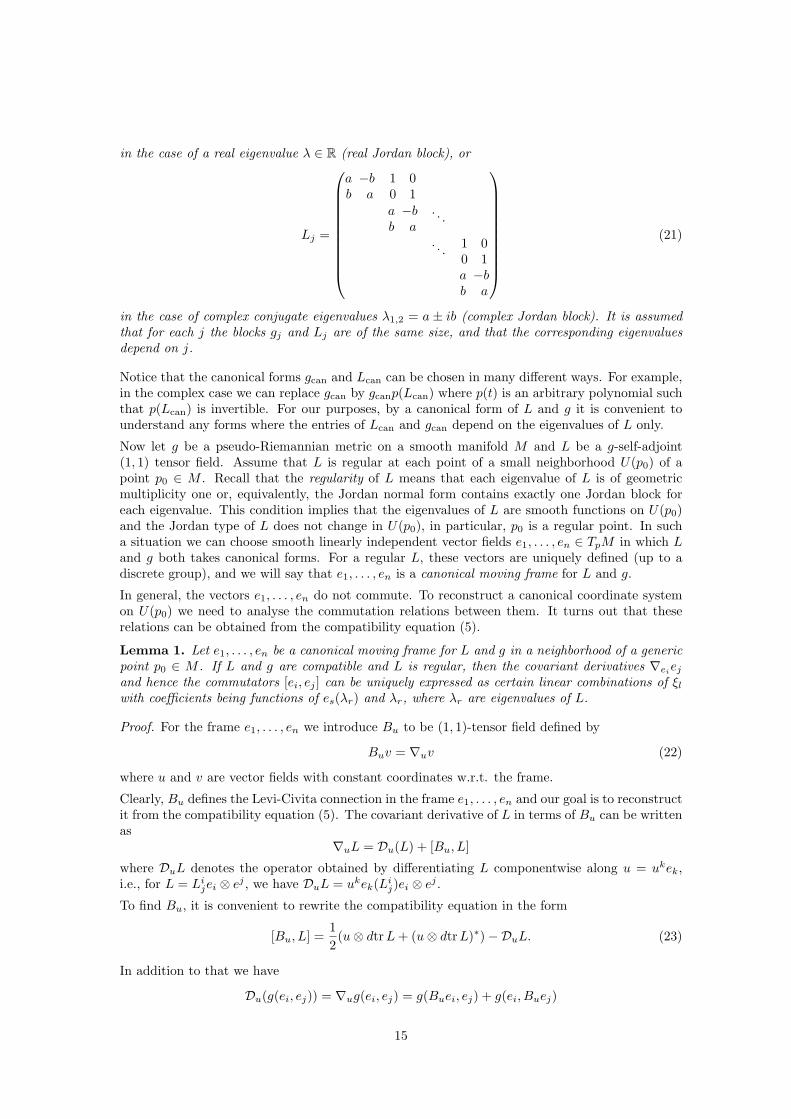
in the case of complex conjugate eigenvalues λ1,2 = a ± ib (complex Jordan block). It is assumedthat for each j the blocks gj and Lj are of the same size, and that the corresponding eigenvaluesdepend on j.
Notice that the canonical forms gcan and Lcan can be chosen in many different ways. For example,in the complex case we can replace gcan by gcanp(Lcan) where p(t) is an arbitrary polynomial suchthat p(Lcan) is invertible. For our purposes, by a canonical form of L and g it is convenient tounderstand any forms where the entries of Lcan and gcan depend on the eigenvalues of L only.
Now let g be a pseudo-Riemannian metric on a smooth manifold M and L be a g-self-adjoint(1, 1) tensor field. Assume that L is regular at each point of a small neighborhood U(p0) of apoint p0 ∈ M . Recall that the regularity of L means that each eigenvalue of L is of geometricmultiplicity one or, equivalently, the Jordan normal form contains exactly one Jordan block foreach eigenvalue. This condition implies that the eigenvalues of L are smooth functions on U(p0)and the Jordan type of L does not change in U(p0), in particular, p0 is a regular point. In sucha situation we can choose smooth linearly independent vector fields e1, . . . , en ∈ TpM in which Land g both takes canonical forms. For a regular L, these vectors are uniquely defined (up to adiscrete group), and we will say that e1, . . . , en is a canonical moving frame for L and g.
In general, the vectors e1, . . . , en do not commute. To reconstruct a canonical coordinate systemon U(p0) we need to analyse the commutation relations between them. It turns out that theserelations can be obtained from the compatibility equation (5).
Lemma 1. Let e1, . . . , en be a canonical moving frame for L and g in a neighborhood of a genericpoint p0 ∈ M . If L and g are compatible and L is regular, then the covariant derivatives ∇ei
ej
and hence the commutators [ei, ej ] can be uniquely expressed as certain linear combinations of ξl
with coefficients being functions of es(λr) and λr, where λr are eigenvalues of L.
Proof. For the frame e1, . . . , en we introduce Bu to be (1, 1)-tensor field defined by
Buv = ∇uv (22)
where u and v are vector fields with constant coordinates w.r.t. the frame.
Clearly, Bu defines the Levi-Civita connection in the frame e1, . . . , en and our goal is to reconstructit from the compatibility equation (5). The covariant derivative of L in terms of Bu can be writtenas
∇uL = Du(L) + [Bu, L]
where DuL denotes the operator obtained by differentiating L componentwise along u = ukek,i.e., for L = Li
jei ⊗ ej , we have DuL = ukek(Lij)ei ⊗ ej .
To find Bu, it is convenient to rewrite the compatibility equation in the form
[Bu, L] =1
2(u ⊗ dtr L + (u ⊗ dtr L)∗) −DuL. (23)
In addition to that we have
Du(g(ei, ej)) = ∇ug(ei, ej) = g(Buei, ej) + g(ei, Buej)
15
or, equivalentlyBu + B∗
u = g−1Dug
Thus, Bu satisfies two equations of the form
[Bu, L] = CBu + B∗
u = D(24)
where C and D are certain operators (whose components w.r.t. the moving frame are functionsof the eigenvalues λr and their derivatives es(λr)).
The uniqueness of the solution (if it exists!) is a purely algebraic fact. Indeed, consider thecorresponding homogeneous system
[Bu, L] = 0Bu + B∗
u = 0(25)
The first equation means that Bu commutes with L, i.e., belongs to the centralizer of L. Since Lis regular, its centralizer is generated by powers of L, i.e., 1, L, L2, . . . , Ln−1. It follows from thisthat Bu is g-selfadjoint. But then the second equation can be rewritten simply as 2Bu = 0. Thus,the homogeneous system has the only trivial solution which proves the statement.
The commutators [ei, ej ] can now be uniquely reconstructed by means of the standard formula:[ei, ej ] = ∇ei
ej −∇ejei = Bei
ej − Bejei.
In the next section we show how the commutation relations between the elements of the canonicalmoving frame can be found in practice.
Notice that Lemma 1 does not say that (24) is always consistent for every C and D. In fact, thesematrices have to satisfy some additional relations (for example, trCLk = 0). These equations, inparticular, imply vanishing of the Nijenhuis torsion of L and, therefore, the fact that es(λr) = 0for those es which “do not belong” to the λr-block. Another condition of this kind is discussedbelow in Lemma 2.
3.2 Canonical frame and canonical coordinate system for a real Jordan
block
Let L be conjugate to a Jordan block with a real eigenvalue. Then we can chose a moving framee1, . . . , en in which L and g take the following canonical forms:
Lcan =
λ(x) 1
λ(x). . .
. . . 1λ(x)
, gcan = ±
11
. ..
1
(26)
Here we apply the ideas from § 3.1 to describe the commutation relations between ξ1, . . . , ξn andthen to solve them in order to construct a canonical coordinate system for the pair g and L.
As usual, it is convenient to decompose L canonically into the semisimple and nilpotent parts:
L = λ(x) · 1 + N.
Obviously, N is self-adjoint with respect to g. The compatibility equation can naturally be rewrit-ten in terms of N :
∇u(L) = u(λ) · 1 + ∇uN =n
2
(u ⊗ dλ + (u ⊗ dλ)∗
)
or[Bu, N ] =
n
2
(u ⊗ dλ + (u ⊗ dλ)∗
)− u(λ) · 1, (27)
16

where Bu, as before, is defined by (22), and we use the fact that the components of N in the frameare all constants so that ∇uN = [Bu, N ]. This equation implies
Lemma 2. We have ei(λ) = 0, for i = 1, . . . , n − 1.
Proof. This property is well known for L with zero Nijenhuis torsion (for L this condition isfulfilled, see e.g. [6, Theorem 1]). However, we can easily derive this fact from (27). Indeed,multiply the both sides of this equation by N and take the trace. For the left hand side we get:
tr(N · [Bu, N ]
)= 0.
For the right hand side:
tr(
N ·(n
2
(u ⊗ dλ + (u ⊗ dλ)∗
)− u(λ) · 1
))
= n · Nu (λ) − u(λ) · trN = n · Nu (λ).
Thus, for any vector v = Nu ∈ Im N , we have v(λ) = 0. It remains to notice that ImN =span(ξ1, . . . , ξn−1).
Thus, in our basis dλ = (0, . . . , 0, en(λ)). This allows us to get the following explicit form for theright hand side of (27):
∇uN = [Bu, N ] = en(λ)
n−22 un
n2 un−1
n2 un−2 . . . n
2 u2 nu1
−unn2 u2
−unn2 u3
. . .
−unn2 un−1n−2
2 un
(28)
According to Lemma 1, the solution of this equation is unique. We just give the final answer(reader can check this result by substitution into (28)).
Bu = en(λ)
n2 un−1
n2 un−2 . . . n
2 u2n2 u1 0
(1 − n2 )un −n
2 u1
(2 − n2 )un −n
2 u2
. . .
(n2 − 2)un −n
2 un−2
(n2 − 1)un −n
2 un−1
(29)
The next step is to find pairwise commutators [ei, ej ].
Lemma 3. The vector fields e1, . . . , en−1 commute.
Proof. Let u = u1e1 + . . . unen. It follows from (29) that
∇uej = en(λ)(n
2un−je1 + (j −
n
2)unej+1
)
, j < n.
Hence ∇eiej = en(λ)n
2 e1 if and only if i + j = n, otherwise ∇eiej = 0. In any case
[ei, ej ] = ∇eiej −∇ej
ei = 0
for i, j < n.
It remains to find the commutators [ei, en].
Lemma 4. For i = 1, . . . , n − 1, we have
[ei, en] = −ien(λ) · ei+1.
17

Proof. From (29) we have
∇eien = −
n
2en(λ) · ei+1 and ∇en
ei = −(i −n
2)en(λ) · ei+1.
Thus,
[ei, en] = −en(λ)(n
2ei+1 + −(i −
n
2)ei+1
)
= −ien(λ) · ei+1,
as stated.
Our goal now is to find a coordinate system with respect to which N and g have the simplestform. Since the vector fields e1, . . . , en−1 commute we can choose a coordinate system x1, . . . , xn
in such a way that e1 = ∂x1, . . . , en−1 = ∂xn−1
. To make our choice unambiguous, we assume thatour point p0 ∈ M has all coordinates zero and, in addition,
en = ∂xnon the xn-axes, (30)
i.e. on the curve x1 = x2 = · · · = xn = 0. Notice that the foliation generated by ImN is given byxn = const and the eigenvalue λ depends on xn only.
To rewrite L and g in this coordinate system we just need to find the transition matrix betweene1, . . . , en and ∂x1
, . . . , ∂xn. Since ∂xi
= ei, i = 1, . . . , n−1, it remains to determine the coefficients(yet unknown) of the linear combination
∂xn= a0e1 + · · · + an−1en
First we use the fact that λ does not depend on x1, . . . , xn−1. Therefore
λ′xn
= ∂xn(λ) = (a0e1 + · · · + an−1en)(λ) = an−1en(λ).
Since ∂xnmust commute with each ei = ∂xi
(i < n), we obtain a system of differential equationson aj :
0 = [ei, a0e1 + · · · + an−1en] =
n∑
l=1
∂al−1
∂xi
· el − an−1 ien(λ) · ei+1 =
n∑
l=1
∂al−1
∂xi
· el − iλ′xn
· ei+1,
or, equivalently,
∂al−1
∂xi
= 0, if l 6= i + 1 and∂ai−1
∂xi
= iλ′xn
, i = 1, . . . , n − 1.
In other words, a0 = a0(xn), whereas ai−1 depends on xi−1 and xn and satisfies the equation
∂ai−1
∂xi−1= (i − 1)λ′
xn, i 6= 1,
which can be easily solved. Its general solution is
ai−1(xi−1, xn) = (i − 1)λ′xn
xi−1 + fi(xn),
where fi(xn) is an arbitrary function. But we have a kind of initial condition (30) that requires
ai−1(0, . . . , 0, xn) = 0 for i 6= n, and an(0, . . . , 0, xn) = 1.
It follows immediately from this that
ai−1 = (i − 1)λ′xn
xi−1, i 6= n, (31)
andan−1 = (n − 1)λ′
xnxn−1 + 1. (32)
18

Thus, the transition matrix C has been found:
(∂x1, . . . , ∂xn
) = (e1, . . . , en) · C, with C =
1 a0
1 a1
. . ....
an−1
and a1, . . . , an defined by (31) and (32).
Now to obtain the form of g and L in the local coordinates x1, . . . , xn, we only need to apply thestandard rule
Lcan −→ L = C−1LcanC, gcan −→ g = C⊤gcanC.
where Lcan and gcan are defined by (26). A straightforward computation of L and g gives thestatement of Theorem 4.
The converse statement easily follows from direct verification (also one may notice that the abovearguments are, in fact, invertible and therefore L and g given by Theorem 4 satisfy the compati-bility equation (5) automatically).
4 Proof of Theorem 5: a pair of complex conjugate Jordan
blocks
In this section we assume that L has two complex conjugate eigenvalues λ = a+ ib and λ = a− ib,b 6= 0 (each of geometric multiplicity one), so that L and g can be simultaneously reduced to thefollowing canonical forms
Lcan =
a −bb a
1 00 1
a −bb a
. . .
. . .1 00 1a −bb a
and gcan =
11
. ..
11
(33)
By using the “moving frame” machinery as above, we can find the commutation relations betweenthe elements of the canonical frame (associated with the canonical forms (33) of L and g) anddescribe the corresponding canonical coordinate system. However, this approach leads to serioustechnical difficulties because the commutation relations turn out to be quite complicated. Tosimplify them we will change the canonical forms L and g in a certain way which is, in fact,motivated by the splitting construction from [9] which we recalled in § 1.2. Namely, we set:
Lcan = Loldcan, gcan = gold
can
((Lold
can − λ · 1)n + (Loldcan − λ · 1)n
), (34)
where Loldcan and gold
can are as in (33), and n = 12 dimM . Notice that the operator
((L − λ · 1)n +
(L − λ · 1)n)
is real, so gcan is a real symmetric matrix.
Let e1, f1, e2, f2, . . . , en, fn be the canonical frame associated with these (real) canonical forms.To simplify the commutation relations between them, we need one more modification. Namely,we pass from ei, fi (i = 1, . . . , n) to the natural complex frame ξ1, . . . , ξn, η1, . . . , ηn by putting
ξk =1
2(ek − ifk), ηk =
1
2(ek + ifk) = ξk, (35)
Thus, from now on we allow ourselves to use formal complex combinations of tangent vectors, i.e.,we pass from the real tangent bundle TM to its complexification T CM . In particular, we consider
19

the complex vector fields ξ = e + if , e, f ∈ Γ(TM), and treat them as differential operators onthe space of complex-valued smooth functions w(x) = u(x) + iv(x) on M :
ξ(w) = (e(u) − f(v)) + i(e(v) + f(u)).
The commutators of complex-valued vector fields and other objects of this kind are defined in thenatural way.
According to Lemma 1, we now can uniquely reconstruct the commutation relations between theelements of the frame ξ1, . . . , ξn, η1, . . . , ηn and information about derivatives of λ and λ alongthese elements. Here is the result
Proposition 3. Let e1, f1, e2, f2, . . . , en, fn be the canonical frame associated with canonical forms(34). Then the complex frame
ξ1, . . . , ξn, η1, . . . , ηn
defined by (35) satisfies the following properties:
1. ξk and ηm commute for all k,m;
2. ξ1, . . . , ξn−1 commute and η1, . . . , ηn−1 commute (in particular, all real vector fields ek andfm commute for all k,m ≤ n − 1);
3. the only non-trivial derivatives are ξn(λ) and ηn(λ);
4. non-trivial commutation relations are:
[ξ1, ξn] = − ξn(λ) · ξ2, [η1, ηn] = − ηn(λ) · η2,[ξ2, ξn] = −2ξn(λ) · ξ3, [η2, ηn] = −2ηn(λ) · η3,[ξ3, ξn] = −3ξn(λ) · ξ4, [η3, ηn] = −3ηn(λ) · η4,. . . . . .[ξn−1, ξn] = −(n − 1)ξn(λ) · ξn, [ηn−1, ηn] = −(n − 1)ηn(λ) · ηn.
Proof. One can find these relations by straightforward (linear-algebraic) computation, but weshall give another proof based on the splitting construction (see §1.2) and the uniqueness lemma(Lemma 1).
Before discussing the case of a complex Jordan block (more precisely, of two complex conjugateblocks), consider the case of two real Jordan blocks with distinct eigenvalues as an illustratingexample. Take two compatible pairs (g1, L1) and (g2, L2), each of which represents a single Jordanblock with eigenvalue λi ∈ R (see the previous section for complete description). Let ξ1, . . . , ξn
be the canonical frame for the first pair (g1, L1) and η1, . . . , ηk for the second one (g2, L2). Thegluing lemma (Theorem 1) allows us to construct a new compatible pair L, g by putting:
L =
(L1 00 L2
)
, g =
(g1χ2(L1) 0
0 g2χ1(L2)
)
=
(g1 00 g2
)
(χ1(L) + χ2(L)) (36)
where χi(t) is the characteristic polynomial of Li. The compatibility of Li and gi, i = 1, 2,guarantees the compatibility of L and g.
Now ask ourselves the converse question. Let ξ1, . . . , ξn, η1, . . . , ηk be the canonical frame for acompatible pair g, L having the (non-standard) canonical form (36) with Li, gi being the standardcanonical forms as (26). What are commutation relations between the elements of the frame andconditions on the derivatives of the eigenvalues λ1 and λ2 along the frame? We mean, of course,those relations which can be derived from the compatibility equation for g and L.
Using the uniqueness result (Lemma 1), we immediately conclude that these relations will beexactly the same as for two separate Jordan blocks, namely, ξi’s commute with ηj ’s and therelations within each of these two groups will be those given in Lemmas 3 and 4.
20

We now notice that in this construction noting changes if we allow λ1 and λ2 to be complexconjugate, i.e., λ1 = λ and λ2 = λ, Imλ 6= 0. The elements ξ1, . . . , ξn, η1, . . . , ηk of the canonicalframe will be, of course, vectors of the complexified tangent space (TP M)C. The point is thatLemmas 1, 2, 3 and 4 are of purely algebraic nature and therefore can be applied for comlexifiedobjects without any change.
If e1, f1, e2, f2, . . . , en, fn is the canonical frame associated with the (real) canonical forms (34),then in the complex frame ξ1, . . . , ξn, η1, . . . , ηn defined by (35), Lcan and gcan take the form:
Lcan 7→ L′can =
λ 1
λ. . .
. . . 1λ
λ 1
λ. . .
. . . 1λ
=
(Lλ 00 Lλ
)
,
gcan 7→ g′can =1
2
−i
. ..
−ii
. ..
i
·(χ1(L
′can) + χ2(L
′can)
),
where χ1(t) = (t − λ)n and χ2(t) = (t − λ)n are the characteristic polynomials of Lλ and Lλ
respectively.
According to Lemma 1, we now can uniquely reconstruct the commutation relations between theelements of the frame ξ1, . . . , ξn, η1, . . . , ηn and information about derivatives of λ and λ alongthese elements. This reconstruction can be done by straightforward computation, but we do notneed to repeat it once again. Instead it suffices to notice that we are now exactly in the samesituation as in the case of two real Jordan blocks, see formula (36) and discussion around. So wecan repeat the above argument to get the conclusion of Proposition 3.
The canonical coordinate system x1, y1, x2, y2, . . . , xn, yn can now be reconstructed from theserelations. To do it in the most natural way, notice that L induces a complex structure J on M .Indeed, we can introduce J in the invariant way as follows. Let L = Ls + Ln be the canonicaldecomposition of L into semisimple and nilpotent parts. Then J = 1
b(Ls − a) where λ = a + ib is
the eigenvalue of L. It is easy to see that J2 = −1 and the integrability of J , i.e., vanishing of itsNijenhuis torsion N(J) follows from the same condition for L.
Remark 7. The fact that the Nijenhuis torsion N(L) of L vanishes is well known (see e.g. [6]),the implication N(L) = 0 ⇒ N(J) = 0 can be verified directly. Alternatively, one can use [9,Lemma 6]. Indeed, J can be represented as J = f(L) where f is the analytic (locally constant!)function defined on C \ R in the following way: f(a + ib) = i if b > 0 and f(a + ib) = −i if b < 0.
For the basis vectors ξk and ηk we have Jξk = iξk and Jηk = −iηk. This means that for anyholomorphic coordinate system z1, . . . , zn, the vectors ξk’s are linear combinations of ∂zk
and ηk’sare linear combinations of ∂zk
. Moreover, item 1 of Proposition 3 says that the vector fieldsξ1, . . . , ξn are holomorphic.
From now on we can forget about ηk’s and work with ξk’s only. The following repeats the argumentsfor the real Jordan blocks, but in the complex (holomorphic) setting. Since the holomorphic vector
21

fields ξ1, . . . , ξn−1 pairwise commute we can find a local complex coordinate system z1, . . . , zn suchthat
ξk = ∂zkk = 1, . . . , n − 1
Moreover, this coordinate system can be chosen in such a way that on the two-dimensional surfacez1 = z2 = · · · = zn−1 = 0, we have
ξn = ∂zn. (37)
The eigenvalue λ is a holomorphic function (since ξk’s are holomorphic and [ξn−1, ξn] = −(n −1)ξn(λ) · ξn). Moreover, λ depends of zn only because ξk(λ) = ∂zk
(λ) = 0, k = 1, . . . , n − 1.
Now our goal is to determine the transition matrix between two bases ξ1, . . . , ξn and ∂z1, . . . , ∂zn
,.As before, we consider the relation
∂zn=
n∑
k=1
ak−1ξk =n−1∑
k=1
ak−1∂zk + an−1ξn.
Applying this differential operator to λ we obtain:
λ′zn
=∂λ
∂zn
= an−1ξn(λ)
Next applying it to zk, k = 1, . . . , n − 1, we see that ak depends on zk and zn only and satisfies:
∂ak
∂zk
= kan−1λ′ = k
∂λ
∂zn
.
These equations can be easily solved:
ak = kzk
∂λ
∂zn
+ hk(zn, zn)
And taking into account the initial conditions (37), we conclude that
a0 = 0,
a1 = λ′zn
z1,
a2 = 2λ′zn
z2,
. . .
an−2 = (n − 2)λ′zn
zn−2,
an−1 = 1 + (n − 1)λ′zn
zn−1.
(38)
These formulas are, of course, identical to those for the real case. The only difference is that nowwe work with complex variables.
Now we have all the information to rewrite the formulas for L and g in the basis ∂zi. Notice that
L commutes with the complex structure J and therefore L can be treated as a complex operator.The form g is also compatible with J in the sense that g(Ju, v) = g(u, Jv) so that g can beunderstood as the real part of the complex form on TP M treated as an n-dimensional complexspace (w.r.t. J). This allows us to represent L and g by n×n complex matrices. In the canonicalframe ξ1, . . . , ξn these matrices are:
LC
can =
λ 1
λ. . .
. . . 1λ
22

gC
can =
−i
. ..
−i
· (LC
can − λ · 1)n
To determine L and g (more precisely their complex representations LC and gC) in the coordinatesz1, . . . , zn, we use the standard transformation:
LC
can 7→ LC = C−1LC
canC, gC
can 7→ gC = C⊤gC
canC
with the transition matrix C
(∂z1, . . . , ∂zn
) = (ξ1, . . . , ξn)C, C =
1 a0
1 a1
. . ....
1 an−2
an−1
where ak are defined by (38).
Now a straightforward computation of gC and LC immeditely leads to the conclusion of Theorem5.
5 Applications: some global results
Here we give the proofs of Theorem 6 and Corollary 1.
5.1 Proof of Theorem 6
Consider two projectively equivalent pseudo-Riemannian metrics g and g on M and the (1, 1)-tensor fields L = L(g, g) defined by
Lij =
(det g
det g
) 1n+1
gikgkj .
Theorem 6 can be reformulated as follows:
If M is compact, then L has no non-constant complex eigenvalues. In other words, complexeigenvalues of L are all constant.
The idea of the proof is very natural. As we know from § 4, the complex eigenvalue is a holomorphicfunction in an appropriate coordinate system. Roughly speaking, our proof is somehow equivalentto saying that “a holomorphic function on a compact manifold has to be constant”. However, tomake sense out of this principle we have to deal with two issues:
• the complex structure J (see Theorem 5 and Section 4) is not globally defined;
• the complex eigenvalues may collide and near the collision points the complex eigenvaluesare not well defined functions (these points should be considered as branching points foreigenvalues).
To avoid these difficulties, we use the following two observations:
• a natural complex structure J is well defined as soon as we have complex eigenvalues evenat collision points,
23

• complex eigenvalues λi of L (which are not well defined at collision points) can be replacedby symmetric polynomials of them, like
∑λi, which are still holomorphic and well defined.
These two ideas are formalized in the following lemma. Let χL(t) be the characteristic polynomialof L. Clearly, the coefficients of χL(t) are smooth real functions on M .
Lemma 5. Let µ0 be a complex root of χL(t) of multiplicity k at a point p0 ∈ M , Im µ0 6= 0.Then in a neighborhood of p0 there is a local coordinate system x1, . . . , xk, y1, . . . , yk, v1, . . . , vl,2k + l = dimM , such that the characteristic polynomial of L admits the following factorization:
χL(t) = pz(t) · pz(t) · qv(t) (39)
wherepz(t) = tk + ak−1(z)tk−1 + · · · + a1(z)t + a0(z)
with coefficients am(z) being holomorphic functions of the complex variables zj = xj + iyj,
pz(t) = tk + ak−1(z)tk−1 + · · · + a1(z)t + a0(z),
andqv(t) = tl + bl−1(v)tl−1 + · · · + b1(v)t + b0(v)
where bm(v) are smooth real valued functions of v1, . . . , vl, and the polynomial pz(t) at the pointp0 takes the form (t − µ0)
k.
Proof. We first notice (exactly in the same way as we did in our splitting construction [9]) thatin a neighborhood of p0 the characteristic polynomial χL(t) can be uniquely factorized into twomonic polynomials of degree 2k and l respectively with smooth real coefficients
χL(t) = χ1(t)χ2(t)
in such a way that the roots of χ1(t) at point p0 are µ0 and µ0, both with multiplicity k. Locally, ina neighborhood of p0 these polynomials do not have common roots. This factorization immediatelylead (see [9, Theorem 2]) to the existence of a coordinate system u1, . . . , u2k, v1, . . . , vl in whichL splits into blocks each of which depend on its own group of coordinates:
L =
(L1(u) 0
0 L2(v)
)
,
so that χ1(t) and χ2(t) are the characteristic polynomials of L1 and L2. In other words, locally wemay think of M with L as a direct product (M1, L1) × (M2, L2) of two “independent” manifoldswith (1,1)-tensor fields on them. We put qv(t) = χ2(t) and continue working, from now on, withthe first factor (M1, L1) only.
In a neighborhood of p0, the characteristic polynomial χ1(t) of L1 admits a further factorization:
χ1(t) = pu(t)pu(t)
into two complex conjugate polynomials with smooth complex valued coefficients satisfying therequired property: at the point p0 we have pu(t) = (t − µ0)
k. So far this construction is purelyalgebraic. But now we need to pass from real coordinates u to complex coordinates z = x + iy insuch a way that the coefficients of p(t) become holomorphic functions of z.
First we construct a natural complex structure J on M1. The spectrum of L1 in the neighborhoodof p0 consists of complex eigenvalues only located nearby either µ0 or µ0. In this case J can bedefined as an analytic function of L1, i.e.,
J = f(L1)
24

Here f : C → C is a locally constant function defined on the disjoint union of two small discsB(µ0) and B(µ0) centered at µ0 and µ0:
f(z) =
{
i, if z ∈ B(µ0),
−i, if z ∈ B(µ0)
For definiteness, we assume that Im µ0 > 0, and Im µ0 < 0
An equivalent definition of J is as follows. Let L1 : V 2n → V 2n be a linear operator whoseeigenvalues are all complex (with non-zero imaginary parts!). We consider the decomposition ofV C into two L1-invariant subspaces U+⊕U− corresponding to eigenvalues of L1 with positive andnegative imaginary parts respectively. Such a decomposition is obviously unique. Now we defineJ to be the multiplication by i on U+ and multiplication by −i on U−. It is easy to see that Vas a subspace of V C is J-invariant, i.e., J gives a well-defined operator on V , satisfying J2 = −1and commuting with L1.
Thus, J = f(L1) is a well-defined almost complex structure in a neighborhood of p0. By Lemma 6from [9], the vanishing of the Nijenhuis torsion of L1 implies the same property for J . Therefore,J is integrable and is indeed a complex structure in a neighborhood of p0.
We now need to show that the coefficients of p(t) are holomorphic with respect to J . Though itcan be done independently, we shall easily derive this property from § 4.
Indeed, in § 4 we have shown that in a neighborhood of every generic point each complex eigenvalueλi of L is a holomorphic function (in the “singular” case studied in § 2, λi is constant, so thisproperty holds automatically). On the other hand the coefficients aj(z) of pz(t) are symmetricpolynomials in λi, so they are holomorphic at each generic point too. Now it remains to noticethat generic points form open everywhere dense subset and aj(z) are smooth everywhere. Thisobviously implies that aj(z) are holomorphic on the whole neighborhood of p0. This completesthe proof.
Remark 8. In the final part of the proof we have used the fact that the complex structure J isin natural sense compatible with the complex structures defined in § 4 (cf. Remark 7). Moreprecisely, in a neighborhood of a generic point, J from Lemma 5 is the direct sum of the complexstructures constructed for each individual (λi, λi)-block by the method explained in § 4. Therefore,“holomorphic on a single complex Jordan block” implies “holomorphic on the sum of all complexJordan blocks”.
We also shall use the following almost obvious statement.
Lemma 6. Let pz(t) = tk+ak−1(z)tk−1+· · ·+a1(z)t+a0(z) be a polynomial in t whose coefficientsare holomorphic functions of z = (z1, . . . , zk) ∈ U , where U ⊂ C
k is an open connected domain.
Assume that at some point z0 ∈ U the polynomial takes the form pz0(t) = (t − µ0)
k and at anyother point z ∈ U all the roots λi(z) of pz(t) satisfy the condition
Im λi(z) ≤ c = Imµ0, i = 1, . . . , k.
Then λi(z) ≡ µ0 for all z ∈ U , i.e., the roots of pz(t) are all constant and equal to µ0. Inparticular, pz(t) ≡ (t − µ0)
k on U .
Proof. Consider the sum∑k
i=1 λi(z) of the roots of pz(t). Since∑k
i=1 λi(z) = −ak−1(z), this sum is
a holomorphic function on U . On the other hand, we see that Im(−ak−1(z)) = Im(∑k
i=1 λi(z))
≤
k · c and Im(−ak−1(z0)) = k · c, i.e., the imaginary part of the holomorphic function −ak−1(z)attains maximum at a certain point z0 ∈ U . This implies (by maximum principle) that ak−1(z) isconstant on U . From this, in turn, it is easy to derive that the imaginary part of each λi(z) and,therefore, λi(z) itself is constant.
We are now ready to complete the proof of Theorem 6.
25
Consider the roots λ1(P ), . . . , λn(P ), n = dimM of the characteristic polynomial χL(t) at P ∈ Mand let
c = maxP∈M, i=1,...,n
Imλi(P )
We assume that some complex eigenvalues exist, so c > 0.
Since the roots λi(P ) depend on P continuously (in natural sense) and M is compact, then c isattained, i.e., there is a point Q ∈ M at which χL(t) has a complex root µ0 such that Imµ0 = c.In general, µ0 may have different multiplicities at different points. Let k be maximal multiplicityof µ0 on M .
Consider the following subset A ⊂ M :
A = {Q ∈ M | µ0 is a root of χL(t) of multiplicity k at the point Q}.
By our assumption A is not empty, and the standard continuity argument shows that A is closed.Let us show that A is open. Indeed, let p0 ∈ A. We first apply Lemma 5 at this point toget the factorization (39) in some neighborhood U(p0), and then apply Lemma 6 to see thatχL(t) = (t − µ0)
k(t − µ0)kqv(t) on U(Q)/ In other words, µ0 is a root of χL(t) of multiplicity k
for all points P ∈ U(Q), i.e. U(Q) ⊂ A and therefore A is open.
Thus, A is open, closed and non-empty. Hence, A = M and we see that χL(t) = (t − µ0)k(t −
µ0)kq(t) everywhere on M . In other words, µ0 is a constant complex eigenvalue of L of multiplicity
k on the whole manifold M .
If q(t) has some complex roots at some points of M , we simply repeat the same argument to showthat these roots have to be constant. This completes the proof of Theorem 6.
Remark 9. The proof is based on the fact that the Nijenhuis torsion of L vanishes identicallyon M . This condition itself implies the conclusion of Theorem 6. In other words, one can provethe following more general fact: if the Nijenhuis torsion of L vanishes identically on a compactmanifold M , then the complex eigenvalues of L have all to be constant.
5.2 Proof of Corollary 1
Thus, we need to prove the following result:
Let M3 be a closed connected 3-dimensional manifold. Suppose g and g are geodesically equivalentmetrics on it. Suppose L given by (2) has a complex (= not real) eigenvalue α+ iβ at least at onepoint. Then, the manifold can be finitely covered by the 3-torus.
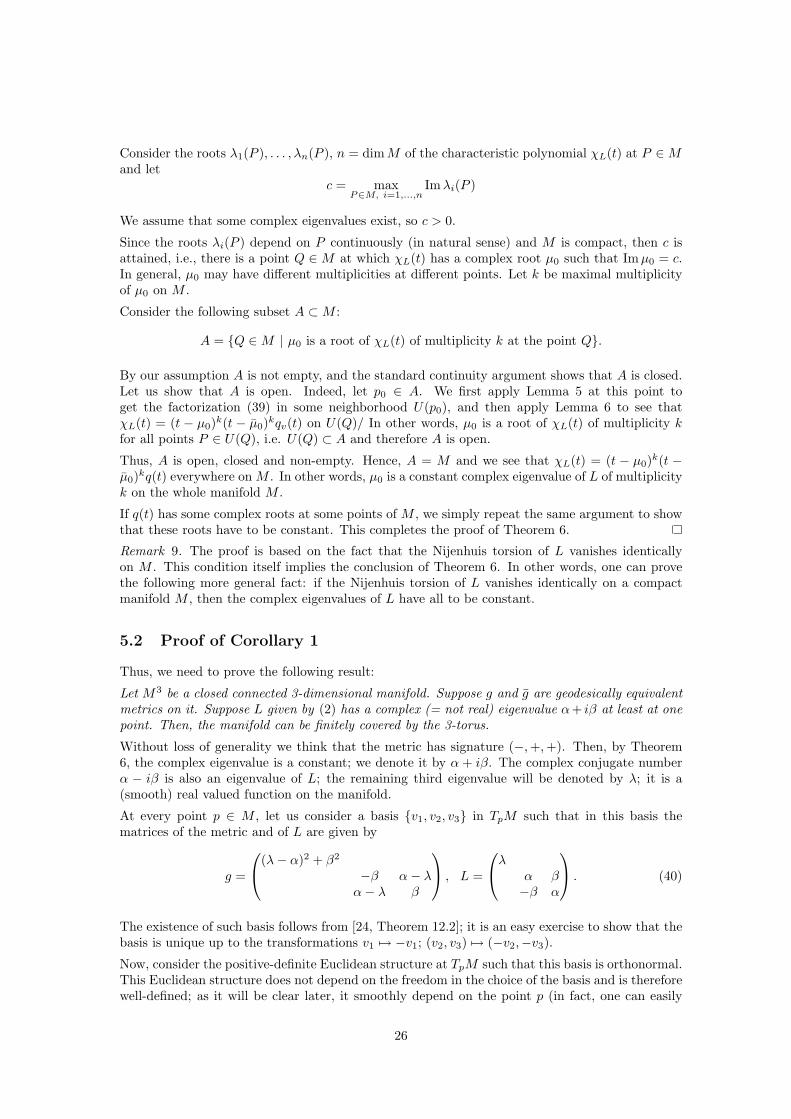
Without loss of generality we think that the metric has signature (−,+,+). Then, by Theorem6, the complex eigenvalue is a constant; we denote it by α + iβ. The complex conjugate numberα − iβ is also an eigenvalue of L; the remaining third eigenvalue will be denoted by λ; it is a(smooth) real valued function on the manifold.
At every point p ∈ M , let us consider a basis {v1, v2, v3} in TpM such that in this basis thematrices of the metric and of L are given by
g =
(λ − α)2 + β2
−β α − λα − λ β
, L =
λα β−β α
. (40)
The existence of such basis follows from [24, Theorem 12.2]; it is an easy exercise to show that thebasis is unique up to the transformations v1 7→ −v1; (v2, v3) 7→ (−v2,−v3).
Now, consider the positive-definite Euclidean structure at TpM such that this basis is orthonormal.This Euclidean structure does not depend on the freedom in the choice of the basis and is thereforewell-defined; as it will be clear later, it smoothly depend on the point p (in fact, one can easily
26
show the smoothness using the implicit function theorem) and therefore generates a Riemannianmetric on M which we denote by g0. Let us show that the metric g0 is flat.
In order to do it, we will use our description of the compatible pair (g, L). As we explained in§1.2, in a neighborhood of every point the metric g could be obtained by gluing (I, h1, L1) and(U2, h2, L2) such that
• I is one-dimensional, the metric g1 is positively definite, and the eigenvalue of L1 is λ.
• U2 is two-dimensional, g2 has signature (−,+) and the eigenvalues of L2 are α + iβ, α− iβ.
Then, for the certain choice of the coordinate x1 on I the metric g1 is (dx1)2 and the only
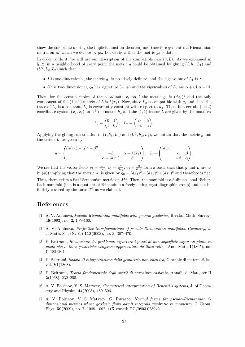
component of the (1× 1)-matrix of L is λ(x1). Now, since L2 is compatible with g2 and since thetrace of L2 is a constant, L2 is covariantly constant with respect to h2. Then, in a certain (local)coordinate system (x2, x3) on U2 the metric h2 and the (1, 1)-tensor L are given by the matrices
h2 =
(0 11 0
)
, L2 =
(α β−β α
)
.
Applying the gluing construction to (I, h1, L1) and (U2, h2, L2), we obtain that the metric g andthe tensor L are given by
g =
(λ(x1) − α)2 + β2
−β α − λ(x1)α − λ(x1) β
, L =
λ(x1)α β−β α
.
We see that the vector fields v1 = ∂∂x1
, v2 = ∂∂x2
, v3 = ∂∂x3
form a basic such that g and L are as
in (40) implying that the metric g0 is given by g0 = (dx1)2 + (dx2)
2 + (dx3)2 and therefore is flat.
Thus, there exists a flat Riemannian metric on M3. Then, the manifold is a 3-dimensional Bieber-bach manifold (i.e., is a quotient of R
3 modulo a freely acting crystallographic group) and can befinitely covered by the torus T 3 as we claimed.
References
[1] A. V. Aminova, Pseudo-Riemannian manifolds with general geodesics, Russian Math. Surveys48(1993), no. 2, 105–160.
[2] A. V. Aminova, Projective transformations of pseudo-Riemannian manifolds. Geometry, 9.J. Math. Sci. (N. Y.) 113(2003), no. 3, 367–470.
[3] E. Beltrami, Risoluzione del problema: riportare i punti di una superficie sopra un piano inmodo che le linee geodetiche vengano rappresentate da linee rette, Ann. Mat., 1(1865), no.7, 185–204.
[4] E. Beltrami, Saggio di interpetrazione della geometria non-euclidea, Giornale di matematiche,vol. VI(1868).
[5] E. Beltrami, Teoria fondamentale degli spazii di curvatura costante, Annali. di Mat., ser II2(1968), 232–255.
[6] A. V. Bolsinov, V. S. Matveev, Geometrical interpretation of Benenti’s systems, J. of Geom-etry and Physics, 44(2003), 489–506.
[7] A. V. Bolsinov, V. S. Matveev, G. Pucacco, Normal forms for pseudo-Riemannian 2-dimensional metrics whose geodesic flows admit integrals quadratic in momenta, J. Geom.Phys. 59(2009), no. 7, 1048–1062, arXiv:math.DG/0803.0289v2.
27

[8] A. V. Bolsinov, V. S. Matveev, G. Pucacco, Dini theorem for pseudo-Riemannian metrics,Math. Ann. 352(2012), 900–909, arXiv:math/0802.2344.
[9] A. V. Bolsinov, V. S. Matveev, Splitting and gluing lemmas for geodesically equivalent pseudo-Riemannian metrics, Transactions of the American Mathematical Society, 363(2011), no 8,4081–4107, arXiv:math.DG/0904.0535.
[10] Ch. Boubel, The algebra of the parallel endomorphisms of a germ of pseudo-Riemannianmetric, arXiv:math.DG/1207.6544.
[11] R. L. Bryant, G. Manno, V. S. Matveev, A solution of a problem of Sophus Lie: Normalforms of 2-dim metrics admitting two projective vector fields, Math. Ann. 340(2008), no. 2,437–463, arXiv:0705.3592.
[12] R. L. Bryant, M. Dunajski, M. Eastwood, Metrisability of two-dimensional projective struc-tures, J. Diff. Geom. 83(2009), no. 3, 465–499.
[13] G. Darboux, Lecons sur la theorie generale des surfaces, Vol. III, Chelsea Publishing, 1896.
[14] U. Dini, Sopra un problema che si presenta nella teoria generale delle rappresentazioni ge-ografice di una superficie su un’altra, Ann. di Math., ser.2, 3(1869), 269–293.
[15] M. Eastwood, V. S. Matveev, Metric connections in projective differential geometry, Symme-tries and Overdetermined Systems of Partial Differential Equations (Minneapolis, MN, 2006),339–351, IMA Vol. Math. Appl., 144(2007), Springer, New York, arXiv:0806.3998.
[16] L. P. Eisenhart, Non-Riemannian Geometry, American Mathematical Society ColloquiumPublications VIII(1927).
[17] L. P. Eisenhart, The geometry of paths and general relativity, Ann. of Math. (2) 24(1923),no. 4, 367–392.
[18] G. Fubini, Sui gruppi transformazioni geodetiche, Mem. Acc. Torino 53(1903), 261–313.
[19] V. I. Golikov, Geodesic mappings of gravitational fields of general type, Trudy Sem. Vektor.Tenzor. Anal., 12(1963) 79–129.
[20] V. Kiosak, V. S. Matveev, Complete Einstein metrics are geodesically rigid, Comm. Math.Phys. 289(2009), no. 1, 383-400, arXiv:0806.3169.
[21] G. I. Kruckovic, A. S. Solodovnikov, Constant symmetric tensors in Riemannian spaces, Izv.Vys. Uchebn. Zaved. Matematika 1959 no. 3(10), 147–158.
[22] G. I. Kruchkovich, Equations of semireducibility and geodesic correspondence of Lorentzspaces, Trudy Vsecsoyuz. Zaochn. Energet. Inst., 24(1963), 74–87.
[23] J.-L. Lagrange, Sur la construction des cartes geographiques, Noveaux Memoires del’Academie des Sciences et Bell-Lettres de Berlin, 1779.
[24] P. Lancaster, L. Rodman, Canonical forms for hermitian matrix pairs under strict equivalenceand congruence, SIAM Review, 47(2005), 407–443.
[25] T. Levi-Civita, Sulle trasformazioni delle equazioni dinamiche, Ann. di Mat., serie 2a,24(1896), 255–300.
[26] S. Lie, Untersuchungen uber geodatische Kurven, Math. Ann. 20 (1882); Sophus Lie Gesam-melte Abhandlungen, Band 2, erster Teil, 267–374. Teubner, Leipzig, 1935.
[27] R. Liouville, Sur les invariants de certaines equations differentielles et sur leurs applications,Journal de l’Ecole Polytechnique 59 (1889), 7–76.
28

[28] V. S. Matveev, P. J. Topalov, Trajectory equivalence and corresponding integrals, Regular andChaotic Dynamics, 3(1998), no. 2, 30–45, MR1693470, Zbl 0928.37003.
[29] V. S. Matveev, Hyperbolic manifolds are geodesically rigid, Invent. math. 151(2003), 579–609.
[30] V. S. Matveev, On projectively equivalent metrics near points of bifurcation, In “Topologicalmethods in the theory of integrable systems”(Eds.: Bolsinov A.V., Fomenko A.T., OshemkovA.A.; Cambridge scientific publishers), 213–240, arXiv:0809.3602.
[31] V. S. Matveev, Proof of projective Lichnerowicz-Obata conjecture, J. Diff. Geom. 75(2007),459–502, arXiv:math/0407337.
[32] V. S. Matveev, Geodesically equivalent metrics in general relativity, J. Geom. Phys., 62(2012),no. 3, 675–691.
[33] V. S. Matveev, Two-dimensional metrics admitting precisely one projective vector field, Math.Ann. 352(2012), 865–909, arXiv:math.DG/0904.0535.
[34] J. Mikes, Geodesic mappings of affine-connected and Riemannian spaces. Geometry, 2, J.Math. Sci. 78(1996), no. 3, 311–333.
[35] P. Painleve, Sur les integrale quadratiques des equations de la Dynamique, Compt.Rend.,124(1897), 221–224.
[36] A. Z. Petrov, Geodesic mappings of Riemannian spaces of an indefinite metric (Russian),Uchen. Zap. Kazan. Univ., 109(1949), no. 3, 7–36.
[37] N. S. Sinjukov, Geodesic mappings of Riemannian spaces, (in Russian) “Nauka”, Moscow,1979.
[38] A. S. Solodovnikov, Projective transformations of Riemannian spaces, Uspehi Mat. Nauk(N.S.) 11(1956), no. 4(70), 45–116, MR0084826, Zbl 0071.15202.
[39] P. J. Topalov, Geodesic Compatibility And Integrability Of Geodesic Flows, Journal of Math-ematical Physics 44(2003), no. 2, 913–929.
[40] T. Thomas, On the projective theory of two dimensional Riemann spaces, Proc. Nat. Acad.Sci. U. S. A. 31(1945) 259–261.
[41] O. Veblen, T. Thomas, The geometry of paths, Trans. Amer. Math. Soc. 2(1923), no. 4,551–608.
[42] O. Veblen, J. Thomas, Projective invariants of affine geometry of paths, Ann. of Math. (2)27(1926), no. 3, 279–296.
[43] H. Weyl, Zur Infinitisimalgeometrie: Einordnung der projektiven und der konformen Auffa-sung, Nachrichten von der K. Gesellschaft der Wissenschaften zu Gottingen, Mathematisch-Physikalische Klasse, 1921; “Selecta Hermann Weyl”, Birkhauser Verlag, Basel und Stuttgart,1956.
29