Calhoun: The NPS Institutional Archive

Theses and Dissertations Thesis Collection

1968-05

Loading characteristics of a charge-constrained

synchronous generator.

Regan, James Peter

Massachusetts Institute of Technology

http://hdl.handle.net/10945/40082

LOADING CHARACTERISTICS OF A

CHARGE- CONSTRAINED

SYNCHRONOUS GENERATOR

Author:

Thesis Supervisor:

Date Submitted:

James Peter Regan

Prof. J. R. Melcher

May 17, 1968

LOADING CHARACTERISTICS

OF A

CHARGE-CONSTRAINED

SYNCHRONOUS GENERATOR

by

JAMES PETER ' GAN

B.E.E., VILLfu10VA~IVERSITY

(1963)

SUBMITTED TO THE DEPARTMENT OF NAVAL ARCHITECTURE AND MARI NE

ENGINEERING IN PARTIAL FULFILLMENT OF THE REQUIREMENTS OF

THE MASTER OF SCIENCE DEGREE I N EL~CTRICAL ENGINEERING

AND THE PROFESSIONAL DEGREE, NAVAL ENGINEER

at the

MASSACHUSETTS I NSTITUTE OF TECHNOLOGY

May, 1968

Signature of Author • . .. . . . . . . . . . . . . . . . Department of Naval Architecture and Marine Engineering, May 17, 1968

Certified by • . . . . . . . . . . . . . . . . . . . . . . . .

Certified by . • . • • • • • • •

Accepted by . • . . • • • • • •

Thesis Supervisor

. . . . . . . . . . . . .. . . . . . . Reader for the Department

Chairman, Departmental Committee on Graduate Students

. - '

•

ii LIBI~ARY

NAVAL POSTGR .DUATE SCHOO LOADING CHARACTERISTICS OF DUDLEY KNOX LIBRARY MONTEREY, CALIF . 93940 AL POSTGRADUA'TE SCHOOl.

A CHARGE-CONSTRAINED SYNCHRONOUS GENERA~~V "' MONTEREY, CA 93943-5101

BY

JAMES PETER REGAN

ABSTRACT

Submitted to the Department of Naval Architecture and Marine Engineering on ~-iay 17, 1968, in partial fulfillment of the requirements for the Mas­ter of Science Degree in Electrical Engineering and the Professional Degree, Naval Engineer.

Previous electric-field-type electromechanical energy converters have relied on a variable capacitance, with terminal voltage constrained. An electrostatic generator is studied which employs a spatially varying charge distribution with the potential unconstrained. Energy is converted from mechanical to electrical form by means of ·a synchronous interaction between the excitation charge wave on the moving medium and the fixed load. Power output characteristics for both a continuum and discrete loading arrange­ments are derived and analyzed. A study of the effects of discrete loading is essential to understanding operation with a finite number of phases.

It is shown that such generators may be modeled by an equivalent circuit containing a current source in parallel with a characteristic internal capacitance and a load impedance. The values of these circuit elements are determined by the excitation charge wave and geometrical factors such as: load-to-charge wave spacing , charge-to-ground potential distance, and interelectrode spacing and number of phases in the discrete loading case.

For the discretely loaded generator, the output theory is derived by assum­ing the form of the potential distribution along the loading electrodes. The discreteness requires that Four:i.er techniques be used and that the dis­tribution be treated as an infinite sum of spatial harmonics of the funda­mental wavenumber of the exciting charge wave. A six-phase, discretely loaded generator with an -electrode-to-interelectrode width ratio e~ual to 1.54 is analyzed in detail. It is shown that this generator can deliver 75% of the power available from a continuously loaded generator having the same excitation and physical parameters. Data are presented to predict output power for discrete loadings, with the number of phases .varying from five to 42. A six-phase laboratory generator is used to determine the equivalent circuit element values.

The theory predicts the current source magnitude to within 6%. With the stray capacitance due to electrode structure quantified and included, the characteristic internal capacitance is predicted to within 5% by the theory.

Thesis Supervi sor: J ames R. Melcher Title: Associate Professor of Electrical Engineering

•

iii

ACKNOWLEDGEMENTS

The author wishes to express his appreciation to all those

who helped to make the completion of this thesis possible. He

especially thanks Professor James R. Melcher for suggesting this prob­

lem and for guidance and assistance at all stages of the research.

The author particularly appreciates the assistance of Mr. Edmund

B. Devitt, who checked calculations throughout the preparation. He

also wishes to thank Mrs. Evelyn Homes for her efficient typing of this

manuscript, and Mr. Harold Atlas, who provided invaluable assistance

in the construction of the laboratory apparatus.

Grateful thanks are also due my wife, Janet, for her patience and

understanding .

Financial support for this research was provided by the National

Aeronautics and Space Administration and the United States Navy.

I ·~ ..

. .

iv

LIST OF FIGURES

Page No.

2.1 Cross-sectional view of a continuously loaded

generator channel . . . . . . . . . ~ . . . . . . 2.2 Equivalent circuit diagram for a continuously

loaded generator . • . • • • . • . • • . 10

2.3 Plot of generator output versus load conductance. . • 11

3.1 Cross-sectional view of a discretely loaded generator

channel . • • • • • l3a

3.2 Model for potential distribution of one electrode

phase as used in Fourier analysis

3.3 Total assumed potential distribution along load

electrodes for a 6-phase generator •

3.4 Equivalent circuit diagram for a discretely loaded

generator ..

· Curve 3.1 Plot comparing characteristic capacitances of continu­

ously and discretely loaded generators for a

16

. 16

• • 24

range of phases • • • • • • . ~ ~· ' . . . . . . 29

Curve 3.2 Plot comparing optimum power outputs of .continuously

and discretely loaded generators for a range

of phases . • • . • • 30

Curve 3.3 Plot of discretely loaded generator utilization

efficiency for a range of phases . . . . • . • 31

4.1 Detail sketch of electrode attachment to the load

section of the experimental generator.

4.2 Illustration of the structural capacitance inherent to

the experimental generator • • • • •

Curve 4.1 Plot of the surface charge distribution on the charge

disk of the experimental generator •

• 38

• • 38

• • 43

v

(List of Figures continue d )

Curve 4.2 Plot showing determination of characteristic capaci­

tance of' experimental generator with purely

resistive loading . • • • • • • . . • • • • • • • • 44

Curve 4.3 Plot showing determination of characteristic capa­

citance of experimental g~nerator with resistive

plus capacitive loading . . . • • 45

Curve 4.4 Plot of power output versus load resistance for the

experimental generator • • 46

A.l Cross-sectional viev of experimental generator . • . . . • • 49

A.2 View illustrating the plexiglas layer above the

load electrodes in the experimental generator .••• 50

A.3 View illustrating the asymmetric channel and plexi-

glas charge disk of the experimental generator. 53

B.l Illustration of the plexiglas load and charge wave

disks of the experimental generator

B.2 Photographs of the experimental generator showing

electrode phases loaded in parallel (a)

and individually (b) ••.••.••

58

59

vi

TABLE OF CO~TENTS

Page No.

TITLE PAGE • . . . • . . . . . . . • . • . . . . . . . . • . . i

ABSTRACT ii

LIST OF FIGURES

ACKNOVlLEDGMENTS . . . . . . . . . . . . . . . . . . . . . . . . iv iii

CHAPTER I., Introduction and Background ••.•...•••••• 1

CHAPTER II. , Continuous Loading . . • • • • . • . • • • • • • • • 6

· a) Introduction . . . . . . • • . . . • . . . . . . • . • 6

b) Governing Equations . ~ • • • • • . . • • • . • • • • • • 6 ··

c) Boundary Conditions .•. •. . . 7

d) Solutions . . . .. . . . . 8

e) Equivalent Circuit 9

f) Power Output Calculation 11

g) Power Optimization . • • 11

CHAPTER III., Discrete Loading . 13

a) Introduction . . . . 13

b) Voltage Distribution Model

c) Fourier Analys~s •••

d) Governing Equations

e) Boundary Conditions ..

• 13

. . 17

. . . 18

. . 19

f) Solutions . . . . . . . . . . . . . . . . . . . . . 20

g)

h)

i)

Equivalent Circuit

Power Output • • . •

Power Optimization . . . . . . . . . . . j) Comparison of Discrete and Cont inuous l y Loaded

Generators .

20

• 24

25

• • • . 25

vii

CHAPTER IV., Experiment a l Comparison with Theoreti cal Prediction •.• 32

a)

b)

c)

d)

e)

f)

Introduction • . • • • • • • . . . . . . . . . . . . . . Short Circuit Current Heasurement and Char ge Prediction. •

Evaluation of I~ternal Capacitance Predicted by Theory.

Sources of Capacit cnce Not Accounted for in Theory.

Prediction of Matching Load . • • • . • • • . • • •

Experimenta l I2termination of a Matched Load

g) Discussion of Results . . . . . . . . . .

CHAPTER V., Conclusions •••••• . . . . .. . . . . . . .

• • 32

. . 33

36

37

39

• 40

• 42

47

APPENDIX A, Modifications to Theory for Experimental Generator • . • • 49

a)

b)

c)

Introduction . . . . . . . . . . . . . . . Effect of Plexi glas Layer Above Electrodes . . . . . . . Effect of Asymmetric Loading and Plexi glas Char ge Disk

49

• 50

52

APPENDIX B, EX"Oerimental Generator • • . -· • • • • • • • • • • • • • · • 55

a)

b)

General Generator Arrangement

Measurement of Disk Charge Density •.•

APPENDIX C, Computer Progr ams •••••••••••••

55

57

. . • • • 60

REFERENCES . . . . . . . . . . . . . . . . . . . . . . . . . . .. 63

CHAPTER I

INTRODUC'l'ION AliJ D BACKGROUND

The past several dec~des h~ve seen tne development of electromechanical

energy conversion machinery which has provided our industrial societies with

a means for rapid technological growth. The scientists who experimented with

electrical phenomena a century ago would not have predicted the posture of

electricity in today's ~orld, even in their most optimistic dreams. Since

its implementation, electrical power has become an integral part of man's

daily activity.

Tne dependence of modern society on electric machinery is due to strong

economic factors. Kinetic energy from a natural water fall may be converted

cheaply and efficiently to electrical energy and then transmitted, with small

loss, over great distances to industrial and population centers s o as to pro-

vide useful work.

With relatively few exceptions, magnetic fields sei~e as the energy

coupling mechanism for modern electromechanical energy conversion equipment.

Until recently, the development of electric-field-b?sed energy conversion

machinery as a practical source of significar.t amounts of electrical power

has received only passing interest. Historically, electric-field energy

conversion devices w0re of great interest to those most intently involved

in the development of electrical science dllring the nineteenth century.

These machines were for the most part direct current generators vli th an

energy storage capability, and were employed principally as experimental

laboratory apparatus. (9 ) 'l'he twentieth century thus far has sP.en the Van

de Graaff high-voltage direct current generator as :probably the most signi-

ficant develcpment in electric-field energy conversion machinery.

•

- 2-

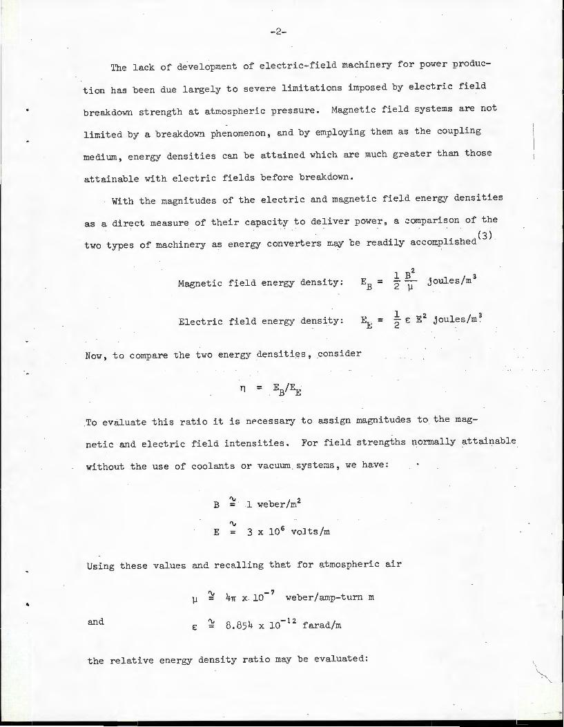
The lack of development of electric-field machinery for powe r produc-

tion has been due largely to severe limitations imposed by electric field

breakdown strength at atmospheric pressure. Magnetic field systems are not

limited by a breakdow~ phenomenon, and by employing them as the coupling

medium, energy densities can be attained which are much greater than those

attainable with electric fields before breakdown.

With the magnitudes of the electric and magnetic field energy densities

as a direct measure of their capacity to deliver power, a ~omparison of the

t t f h . rt '"' d.l l. h d( 3 ) wo ypes o mac lnery as energy conve ers may ~ e rea l y accomp lS e

Magnetic field energy density: joules/m 3

Electric field energy density:

Nm-T , to compare "the two energy densi ti <=s , consider

n =

.To evaluat e this r at io it is nPcessary to assign magnitudes to the mag-

netic and electric field intensities . For field strengths normally attainable

without the use of coolants or vacuum systems, vre have:

B 1 weber/rr?

"v

E = 3 x 10 6 voJts/m

Using these values and recalling that for atmospheric air

and

"v lJ 4 -7

iT X 10 weber/amp-turn m

£ "' 8. 854 x 10- 12 f a r ad/m

the relative energy density ratio may be evaluate d :

"' '/

-3-

This calculation has expose d the advantage which has propelled magnetic

field equipment i nto its present monopolistic position among low-frequency

electromechanical energy conversion machinery.

However, modern technology has made available high vacuum systems and

techniques for efficiently employing them which promote a questioning atti-

tude toward the efficacy of the above energy density comparison. In a high-

( '7) vacuum environment, it has been demonstrated that an improvement by a

factor of 30 in electric field breakdown strength is not out of reach.

In light of this information it is important to ask the question, "If

given a very large electric field energy density, can it be practically em-

played in a generator as the coupling medium for power production?" It is

with the objective of answering this question, at least partially, that this

paper is being prepared . .

The impetus for the research was provided by the recent work done inves-

tigating electrofluid-dynamic (EFD) power sources, conducted by the Continuum

Electromechanics Group here at M.I.T. In turn, the need for such equipment

has been supplied by the space industry and their applications for light-

weight electric power generators aboard space vehicles. Electric-field-based

generators offer a distinct advantage in power delivered per unit weight over

their magnetic held counterparts.

An EFD generator, characterized by a high voltage, low current output, was

d d t t d th b . t of two recent '·1.I.T. Theses(lO,ll). propose an cons rue e as e su Jec 1

The scheme employed a high velocity air flow with entrained particles which

were sinusoidally ctar ge d in a corona exciter. The flow, a traveling wave

cf charge, pa ssed from the exciter through a long , slender channel surrounded

-4-

by a conducting medium. The charge wave interacted synchronously vrith the

conductor, converting kinetic energy from the particle flow into electric

energy which was dissipated as heat. The energy conversion interaction used

in this generator is the electric field analogue of the interaction which

converts kinetic energy to electric energy for magnetic field synchronous

machines.

'l'he synchronous electric field generator proposed and built during the

research for this paper resulted from an attempt to model the charged par-

ticle flow realized in the EFD generator in order that loading character-

istics could be studied. Details of the generator built are set forth in

Appendix B. A standing wave of charge density on a rotating disk was used

to approximate a traveling charge wave passing through a long slender chan-

nel. Synchronism was obtained by establishing an integral number of wave-

lengths of charge distribution around the disk periphery.

Other attempts to build electric field synchronous generators are not

unknown. (7) However, these have been voltage-constrained machines deuending

on a spatial rate of change of capacitance to provide the mechanism for

energy conversion. These types of synchronous machines are the electric field

analogue of the synchronous reluctance machinery in the magnetic field system.

'I'he EFD generator discussed and the one built for this thesis research are

charge-constrained synchronous generators requiring ~ s patial gradient in

the exciting charge density, and no spatial capacitance gradient, for energy

conversion. The magnetic field analogue for this machine is what is known

simply as a 'smooth-air-gap synchronous generator'.

It is interesting to note some of the salient advantages that the charge-

-5-

constrained machine possesses over the voltage-constrained machine.

The electrode blade structure in the voltege-constrained machine under­

goes very rapidly alternating electric pressure forces which present

designers with the possibility of an instability occurring in one of sev­

eral possible modes of vibrat ion. The severity of this problem is obvious

when the blade spacing i s of the order of a millimeter and the rotational

speeds approach 30,000 RPM. The torque-time history for such a machine

shows rapid fluctuations due to the time-varying electric traction as the

blades move in and out of each other's influence. Both of these problems

impose severe limitations on the feasibility of high rotational velocity

operation, which is essential to the production of large amounts of power.

In contrast, the charge-constrained synchronous generator does not

require a spatial gr adi ent in capacitance, hence removes these linitations

on the feasibility of high speed operation. For this machine, the elec­

trical traction force on each part of the rotor (and therefore the mechani­

cal torque) is constant in time. Also, the severity of the alternating

pressur2 forces acting on the electrode structure is greatly diminished

with several electrodes per wavelength of induced voltage . For continuous

loading, as is discussed in Chapter II, this effect is even further reduced.

In s ummary , this research concerns itself with a charge-constrained

synchronous gene rator placing particular emphasis on providing a theory by

which the output of such a generator miglrt be predicted from its physical

parameters and charge wave description. An actual generator was built to

allow for a direct comparison of theory and expe riment. Through this com­

parison, it js hoped that a step forward in the development of a new scheme

for the generation of electrical power has been made .

CONTINUOUS LOADING

Introduction:

-6-

CHAPTER II

A detailed analysis of the continuously loaded, charge-constrained

synchronous generator can provide an excellent insight into the energy

conversion interaction involved. ~his development will serve as the basis

for subsequent analysis in Chapter III of the discretely loaded generator.

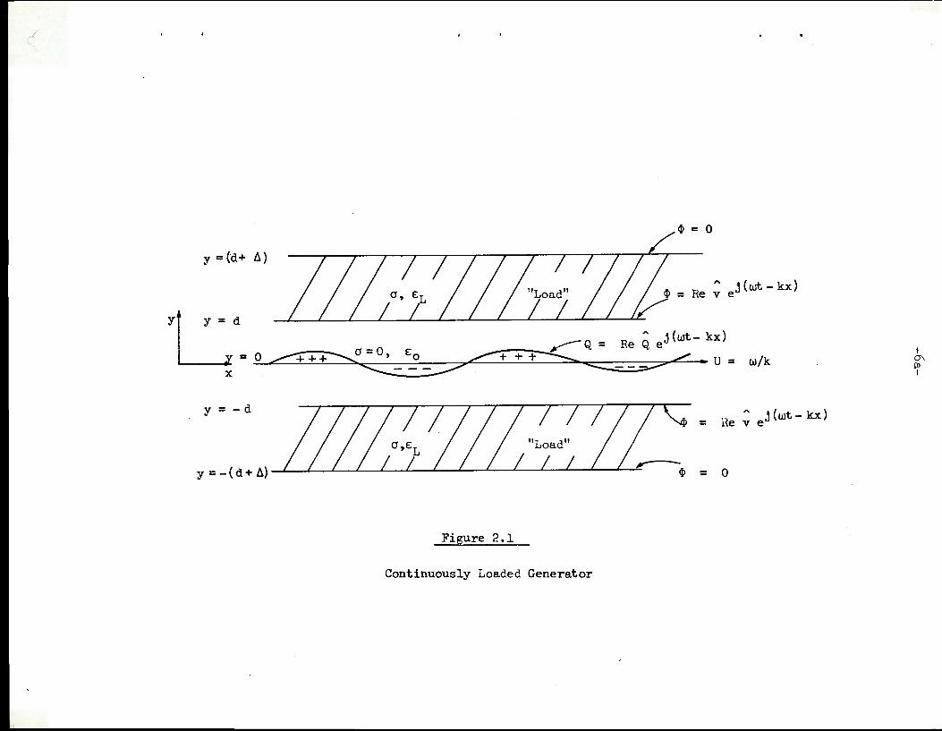
The geometry of the continuously loaded generator will be modeled as shown

in Figure 2.1. The excitation source for this generator is a sheet of

sinusoidally distributed surface charge density traveling along the chan­

nel centerline at a fixed velocity. To an observer fixed in the frame of

the load, this would appear as a t~aveling wave of charg~. The power out­

put of the generator will be measureable in terms of resistive heating in

the conducting load. In this chapter, the source and l0ad will be reduced

to lumped circuit elements normalized to channel load interfacial aree,.

This equivalent circuit approach will prove to be a powerful technique for

studying such a generator ru1d will be extended to the discretely loaded

case in Chapter III.

Governing Equations:

From Fig. 2.l,this problem involves two distinct regions, the lead and

the channel. The most direct method for determination of the fields is to

assume a potential distribution at the load-channel interface, solve the

bulk equations independently in each region, and then match solutions at

the interface. Because of the symmetry of the problem about the y = 0 axis,

it is apparent that the problem need be solved only for the upper region,

with solutions for the lowe r region taking the same form.

_(

$ = 0

y = (d+ t.)

4> = Re ~ ej (wt- kx)

yt y = d

L--r = o ~a=O, e: ,_-Q = Re Q ej(wt- kx) .....:: o ..............-+ + +:::::.......... L -------~ . ............... ;;_;;;;>"- • u = X

w/k

y = - d He ~ e J ( wt - kx )

y=-(d+t.) 0

Figure 2.1

Continuously Loaded Generator

I 0\ Ill I

-7-

From !0:ax:well ' s equation, the gove r ning equat ions for the two regions

of interes t are:

(a) Region (l) 'V2¢ = 0 0 ..5_Y <d c -(2.1)

(b) Region (2) 'V2<P = 0 d. ~y < d + b. L -

Since the potentials in both r egions are established due to the influ-

ence of the traveling wave of charge , t hey will be assumed to be traveling

waves in form also, with the s ame wavenumber as the charge wave . Potential

variations in the z direction may be neglected , as the channel is assumed

slender and ~oride such that 2d/W « l. On this basis, the potential distri-

butions m~st take the form:

= A

Re ¢(y) j (wt - kx) e (2.2)

Substitution of the assumed form of t he potential solution (Eq . 2.2) into

the governing equations (2.1) yields for each region:

(2.3)

The potential solutions therefore are:

(a ) o-:_y2 d

A (2.4)

(b) <PL(y) = AL cosh ky + BL sinh ky d < y 2 d+ b.

Bounda~ Conditions:

Evaluat ion of t he four consta.Dts in equation (2 . 4) ~orill complete the

dete rminat i on of the potential di stribution . This r equi r es four independent

'-.

- 6-

• boundary conditions on the fields . By specifying an assumed potential dis -

t r ibution along the interface as indicated on Fig . 2 . 1, and by specifying

the location of zero potential at the outer boundary of the conductor ,

three boundary conditions are available:

"' (a) ¢c(y=d) = v

"' "' (b) ¢1 (y=d) = v (2 .5)

(c ) ¢1 (y=d + 6) 0

The last boundary condition is obtained from the cha.r ge sheet. At the sheet,

the normal component of the electric field is equal to one-half the magnitude

of the charge density divided by t he dielectric constant. The factor of one-

half is due to the symmetry of the channel; half of the charge excites the

upper region and half excites the lmrer r egion . This boundary condition

becomes:

(d)

Solutions:

d$c<Y~ dy )

y=O

=

Applying the boundary conditions of equation (2.5) to potential solu-

tions expressed in equation (2 . 4) leads to the following matrix equetion for

t he unknown constants.

cosh kd sinh kd 0 0 Ac v

0 1 0 0 Be - Q/ 2£ k 0 (2.6 )

=

0 0 cosh ktl sinh kf:, ~ 0

0 0 1 0 B1 v

- 9-

Evaluation of the constants and substitution into EQuation (2.4) com-

plately specifies the fields in terms of the char ge density and the assumed

potential distribution on the interface .

G, tanh kd] (a) ¢c(y )

v Q cosh ky - Q • h ky = kd + 2£ k 2£ k Sl.n cosh

0 0 (2.7)

A A "' (b) ¢L (y) = v cosh k (y- d)- v coth k6 sinh k (y- d)

E51ui valent Circuit:

Using eQuation (2.7') it is now poss ible to develop an eQuivalent cir-

cuit which characterizes the channel and load interaction. First the load

is characterized by calculating the total current density, conduction current

plus displacement current, which flows into the load region normal to the

interface as a function of the assumed potential distribution . This load

current density is a traveling wave with the s ame wavenumber as that of the

potential and its complex amplitude is given by:

aD~ Tf y=d

oiy) +

fy=d

(a) (2. 8) =

In terms of the potential distribution of eQuation (2.7 b),

(b)

Performing this calculation and defining eQuivalent circuit elements completely

characterizes the load region.

A

JL = [jwC1 + G1 ]V amps / m2 y=d (2 . 9)

where: (a) c :: kc:1

coth k6 farads/m 2 (2.10) L

(b) G = L ok coth kll mhos /m2

-10-

The channel may nm-r be characterized in a manner similar to that used

for the load to obtain the current density normal to the interface out of

the channel reg ion.

" = [- jwCCV + J8

] amns/m2 y=d

where an equivalent capacitance and source have been defined.

(a)

(b) =

ke: tanh kd 0

jwQ 2 cosh kd

farads/m 2

(2.11)

(2.12)

The equivalent circuit may no;.r be obtained by recognizing that there is no

time rate of free surface charge at t he interface, and therefore the current

densities out of and into the interface,as represented by equations (2.9)

and (2.11) respectively,must be equal.

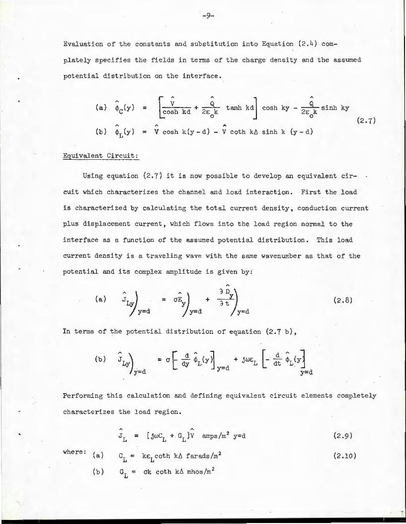
" " = - jw CCV + J 8 (2.13)

'I'he equivalent circuit for the generator which represents the load-channel

interface as a terminal pair is shmm below in Figure 2. 2.

J s

-11-

Power Output Calculation:

The computation of the time average ,ower delivered to the load oL a

per square meter of channel-load interfacial area basis is straightforward,

'\. making use of the equivalent circuit of Figure (2 .2). The power output

found in this •ray is the power delivered to the upper load region only; it is

multiplied by two to account for the lower load. The total power output is:

= I A "*] Re l JG~

In terms of known quantities:

J =

therefore:

. < p >

Power O~timization:

watts/m 2

2 watts/m

(2.14)

(2 .15)

(2 .16)

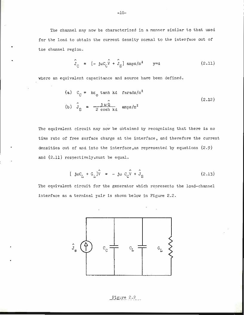
The power output expression of equation (2.16) can be plotted as a func-

tion of load conductance for fixed channel and load geometry and fixed charge

flow condition.

1\

t:Y v I

GL -Fig. 2.3

-12-

From Fig . 2.2, it is obvious that there exists some optimum conduc-

tance GOPT for which the maximum .amount of power is delivered across the

interface to the load. Tc locate this optimum, maximize Equation (2.19)

over GL:

a <P> ----= 0 a GL (2.17)

Carrying out the calculation specified by Equation (2.17) yields:

= (2.18)

The optimum power is obtained by substitution of Eq. (2.18) into (2.16):

(2.19)

It is importan~ to note that Eq. (2.19) is only a limited optimization.

In general,

<P> = (2.20)

This function may be considered as an eight-dimensional vector which

traces some complex surface as the values of the independ~nt variables

are ranged. The absolute optimum power can be found only be considering

all eight variables. The preceding optimization ranged but one variable

couducti vi ty.

Another important factor to take into account when optimizing is the

electric field breakdown strength. (5) It will determine whether or not an

optimum point is indeed physir.ally realizable.

DISCRETE LOADING

Introduction:

-13-

CHAPTER III

The continuously loaded, charge-constrained synchronous generator

analyzed in Chapter II provided a simple mathematical model which placed

particular emphasis on the salient features of generator operation. In

terms of this model, the fundamental energy conversion interaction may be

readily understood. However, as a practical matter, a generator of this

type is of very limited value for use as a source of electrical power.

Most equipment requiring electrical power for operation has discrete elec­

trical terminals, and cannot be considered as a continuous type of load.

Therefore, of more direct interest in determining the feasibility for power

production would be an analysis of a discretely lvaded generator. Rather

than an infinite continuous loading , there would be discrete e:ectrodes of

finite width used to tap off the electrical power, which could then be

transmitted to the locations where electrical machinery and/or equipment

are employed. The nurriller of phases would be determined by the number of

electrodes per wavelength of exciting charge wave.

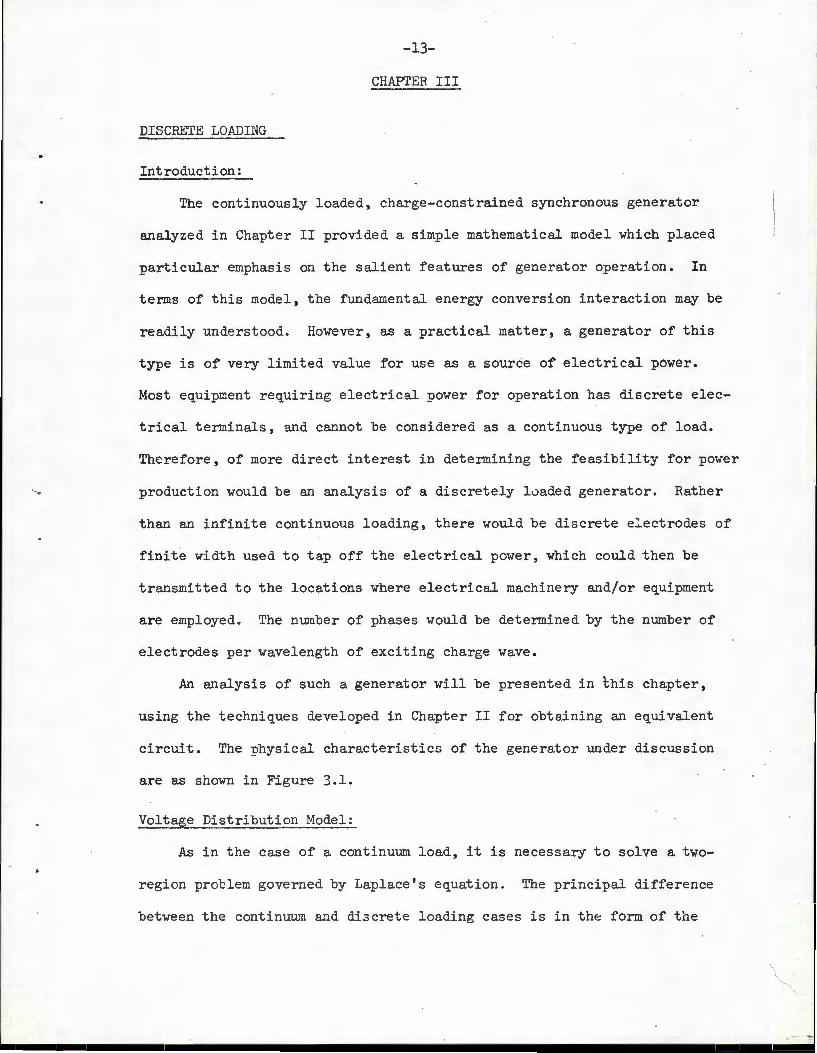
An analysis of such a generator will be presented in this chapter,

using the techniques developed in Chapter II for obtaining an equivalent

circuit. The physical characteristics of the generator under discussion

are as shown in Figure 3.1.

Voltage Distribution Model:

As in the case of a continuum load, it is necessary to solve a two­

region proclem governed by Laplace's equation. The principal difference

between the continuum and diacrete loading cases is in th~ form of the

\

'

,- -

./ ..

Load Impedance.

:'

y=dH I f 11 /$=

0

co yLY = d -L --'- --'- --'- j_ j_ j_ £o $ = Re L $n ej(wt+knxl __ . _L - - n = -co

y = 0 " ~ .c::::::£ · £ ~ Q = Re Q ej(wt-k x)

'""' - - :::;::::>" + + t::::::::,. 0 + 1 Load ~--:..,?'~ u = w/k

• • •

X

Electrode 1

y = - d co ITT-- -- ~ j (wt + ]{ x) Re L A

4> = ql e n n • e • e:

0 n=-co

y =.-(d+l\)) ) ) )

' 4> = 0

depth w

Figure 3.1

Discretely Loaded Generator

I ,_. w sr

'

-14-

potential distribution along the electrodes on the channel boundary. Due

to the finite electrode structure, it is incorrect to assume a potential

wave with the same wavenumber as the exciting charge wave. Rather, spatial

harmonics of the fundamental wavenumber are introduced and the potential

distribution takes the form of a sum of an infinite series of traveling

waves. Thi s allovrs t he problem to be analyzed by means of Fourier tech­

niques.

In order to proceed with a Fourier analysis, it is necessary to obtain

a model for the potential distribution along the channel electrodes. The

first and most obvious constraint on this distribution model is that the

potentiru across e ach electrode must be a constant, since they are assumed

to be perfect conductors. To determine the potential distribution between

adjacent electrodes , to be use d in the model, two possible courses of action

present t hemselves. ~be first is to specify that there is zero net current

density flow normal to the channel axis into the load channel interface.

That is to say, there is no time rate of change of free charge on the inter­

face in the interelectrode regions. 1~e second course of action is to assume

the form of the potential distribution between electrodes, based on physical

reasoning.

With the electrode spacing assumed to be small compared to a wavelength

of the exciting charge wave, a linear potential distribution between elec­

trodes is felt to be a. good approximation, and therefore the second course

of action will be follove d in the ensuing analysis. It is acknowledgEd that

the first alternative would provide a more exact solution; however, the

increased complexity of the problem woul d serve only to confuse, rather than

-15-

to expose the basic principles involved in discrete l oading . It will be

shown in Chapter IV that the r esults pre di cted by this model are reas onably

close to those re alize d from an actual gene rator. It should be note d here

that the slope of the assumed linear distribution must be kept finite, as an

infinite slope such as would result from a stepped potential distribution

, implies an infinite capac itance. Fortunately , as will become clear in the

analysis, tr.e capacitance is not a strong function of slope.

Now that the general form of the potential distribution model has been

determined, the pieces must be put togethe r in such a way as to maintain the

identity of each e l ect rode in the solution. 1~is is desirable, since, when

using the gene r ator, each ele.ctrode' s output must be determinable in terms

of its own loading and that of each of the other electrodes. This may be

accomplished by isolating all electrodes of the s ame phase as a periodic

potential distribution in space, which can then be Fourier-analyzed inde­

pendently of t he electrodes contained in the other phases. The total poten­

tial distribution in space can then be obt aine d by summing these Fourier

series over the numbe r of phases per fund&~ental wavelength. The identity

of each phase is maintained by assigning to it an index. The time frequency

of each Fourier c.:>mponent in this analysis will be ident ical to the time

frequency of t he cha r ge distribution wave .

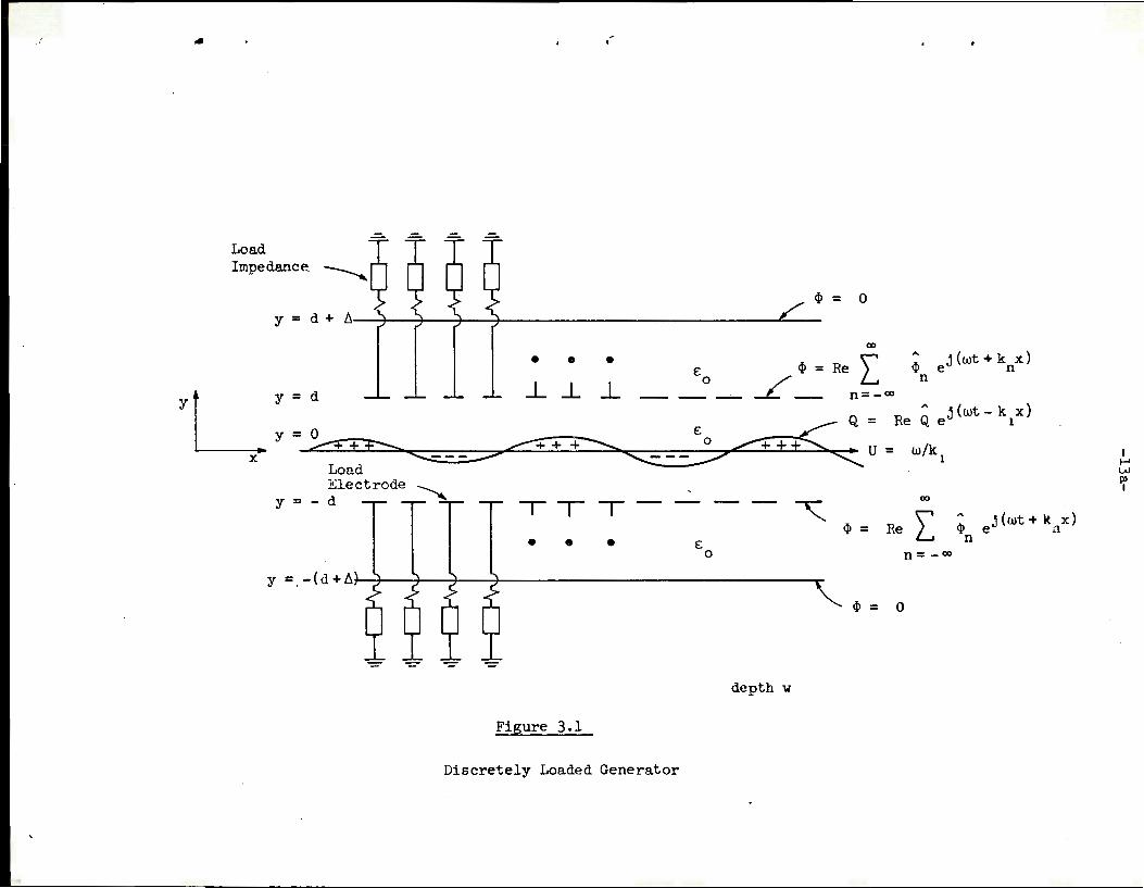
Consider t he case where there are s electrodes pe r fundament al wave­

length, then the pot ential dist ribution associated with the r'th electrode

phase will be assumed to be of t he following form:

' ,

l

jwt e

-16-

Figure 3 . 2

jwt e

jwt e nv

/! l\ r - )"

c = a+ b

.A = sc

X

vr/b[ x-(r-l)c] ( r-1 ) c $ x ~ ( r-1) c + b

v (x) = r

v r

(r-l)c+b ~ x ~ rc (3.1)

rc ~ x . 5 rc + b

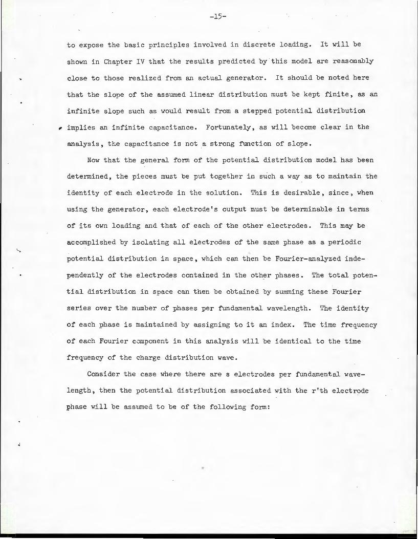
A wave l ength of potenti a l dist ribut i on for t he c ase o f s i x ( 6 ) e l e ctrodes

per wave l ength 1vould t hen have t he following f orm.

v(x)

\ \ \ \

y

Fi gure 3.3

1

\ \ \ \

.A = 6c

X

-17-

Fourier Pnalysis:

In terms of t he pre ceding discussion , the potential distribution on

the electt·ode s may be expre c sed as

s

v(x,t) = Re~ "' jwt v (x)e' r

The compl ex amplitudes are determined from the infinite s ure .

where

v (x) = r

k = n

00

:c L 2rm sc

n= _oo

(3.2)

(3.3)

(3.4)

The ?ourier coefficients for the series (3.3) are obtained from the follow-

ing sum of integrals using Equat ion (3.1).

v = r n

(r-l)c + b

J : [x-(r-l)c]e-jknx dx+

(r-l)c

rc +b

+ [b -x +rc]

rc

-jk X n e dx

rc

(3.5)

Performing t he above-indicated integrations yields the following Fourier

coeffi ci ents for the r'th electrode:

v r

n =

v r knc . .kn

2b]

sin 2 s1n (3.6)

'···

'C

-18-

Using this result togethe r with Equation s (3.2) and (3.3) completely speci-

fies the complex amplitude of the potential distribution along the electrodes

in terms of the assumed model and its phase amplitudes.

s co

v(x) = L L (3.7)

r=l n= - 00

This completes the Fourier analysis and provides the basis for characterizing

the generator by an equivalent circuit.

Governing Equations:

From Fig. 3.1 the symmetry of the generator channel about its center-

line is apparent. It is therefore only necessary to solve the fields prob-

· lem in the upper channel and load region, since the lower solution must take

the same form. The governing equations for the two regions are the s&~e, as

in the case of continuous loading.

(a)

(3.8) (b) d~y~d+!J.

In the preceding section the potential distribution along the load electrodes

was analyzed as an infinite sum of harmonically related traveling waves.

Since the potential in both the channel and load regions must equal the

assumed distribution at the interface, it is efficient to think of the po-

tcntial distribution in these regions as also being made up of an infinite

sum 9f traveling waves, harmonically related to the exciting charge wave.

Each of these harmonics vrill therefore be required to satisfy equation (3.8)

independently. Tha~ is to say, for both regions of interest the potential

~rave will be of the form:

-19-

co

I ex ,y, t) L "' = Re ~ (x ,y, t) (3.9)

n= -co

where "' ej (wt + knx) :tcx,y,t) = ¢ (y)

n (3.10)

For such an anal ysis , the governing equation (3. 8) is also rewritten as:

(a) (3.11)

(b)

Substituting the assumed form for the solution, equation (3.10) into the

governing equation and solving determines the potent ial distribution in

terms of four (4) unknown constants. These constants must be determined

for each harmonic.

(a) ¢n (y) = ~c c cosh knY + Bn sinh kny

c ( 3.12)

(b) ¢n (y) = A cosh kny + B sinh k y L nL nL n

Boundary Condi~ions~_

As with continuous loading ,spe cification of t he potenti a l distribution

along the inte rface and on the outside boundary of the load region rrovides

three (3) of the r equired four boundary conditions . These can bP. expressed

for each harmonic using Equations (3.7) and (3.12).

"' "' (a) ¢ (y=d) = v

nc n

(b) "' "' (3.13) ¢nL (y=d) = v n

(c) ¢n1 (y =d+ M = 0

- 20-

The fourt h boundary condition is proviied by the charge distribut ion, again

as done in the continuous load case. Hmrever, only the fundamental harmonic

is involved in matching the channe l distribution to the exciting charge

wave.

(d) d¢n (y~ = dy

y=O

where: n = - 1

n 'f - l

Solutions:

Application of the boundary conditions expressed in E~uation (3.13)

to the governing e~uation distributions of equation (3.12) completely

specifies the potential distribution in the load and channel regions in

terms of the phase complex amplitudes.

=

A "'·

+ Q o_w J

2E k o n

cosh k y -n'

Qo -1n ---2E k o n

sinh k y n

<P = v [cosh k (y -d) - coth k 6 sinhk (y-d)] nL n n n n

where: s -jknrc A =I V e

[4 jkna/2 k c knb J jk x r sin JL sin v

scbk e -2- e n n 2 n

r=l

as developed in the Fourier analysis section.

Equivalent Circuit:

(3.14)

( 3 .15 )

(3.16)

The ana~ysis involved to obtain an equivalent circuit for the discretely

loaded gene rator is analogous to t hat followed in Chapter II for the continuum

-21-

loaded generator. To characterize the channel and load regions, solve for the

net current density normal to the interface as a function of the potential

distribution along the elect.rodes. Then to include the effect of the lumped

th loading , as shown in Fig. 3.1, consider the ~ electrode and apply conser-

vation of current.

= (3.17)

In the expression the current density is also represented as an infinite

series of harmonically related traveling waves. The complex amplitude for

each harmonic is determined by the l umped circuit chara.cterization of the

load and channel r egions.

"' J = J - j.u [ C + C ]v

n s n n n

The source term is the same form as found in the continuous ca.se.

J = s

jwQo -1n 2

-2--h~k-d amps/m cos n

The lumped capacitance characterizing the channel region is:

c = E: k tanh k d farad/m 2

nc o n n

and that characterizing the load region :

c = E: k coth k /j farad/m2

nL o n n

(3.18)

(3.19)

(3.20)

(3.21)

Interchanging t he order of surrmation and integrat ion in Equation ( 3.17) and

carrying out the integr ation yields:

·'-.. ..

- ,..

-22-

A A

kla/2 00

jk £-c -jk a]

V£,Y£. jwQ sin -jk (£c- a/2 )

L v e n [C + c ~ ][ 1- e n

n nc :nL

= e 1 - w g k cosh k d k

l 1 n n=- oo (3 . 22 )

Equation (3.22) is the most general form of solution for the voltage on the

£th electrode as a function of its load admittance, and t~e voltages and

load admittances of all other s - 1 electrodes. It is convenient to consider

Equat i on (3.22) as a vector equation of the form.

a a l l 12

a 21

or in vector notation:

A V = D

a 15

a ss

where the elements of A are of the form:

={ ;r 0

"' co

+ jWEO I 8V a£r 0~y-[tanh g £-r sc n

n= _ oo

k~cJ} t kna . knb . sin 2

Sln __ Slll 2

A

and of D A jwQ sin k a/2 - j k ( £c - a I 2 )

D£ 1 l e 1 = k cosh k d

l l

knd

A

v D l 1

v D 2 2

= (3.23)

"' "' v D s s _,

(3.24)

jkn (£-r )c + coth knll.]e

(3.25)

(3.26 )

·'--....

- 23-

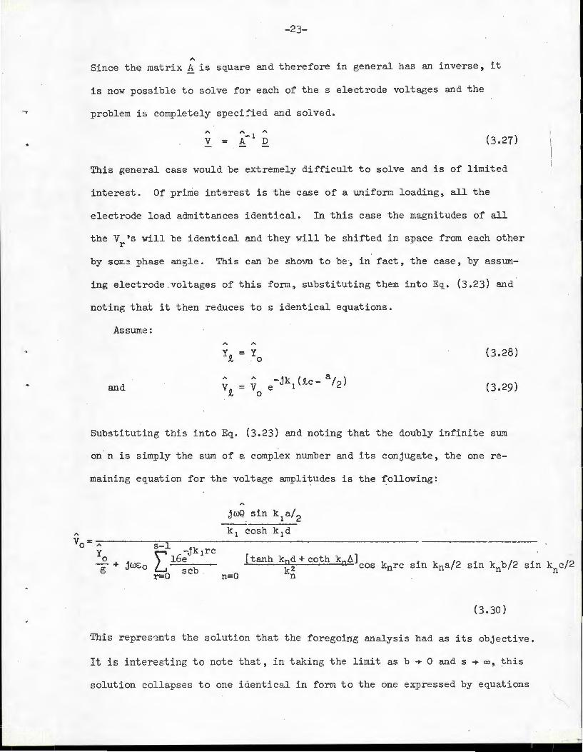
Since the matri x A is square and t here fore in general has an inve-rse , it

i s now possible to solve for each of the s electrode volt aees and the

pr obl em i s completely speci~ied and solved.

v = (3 .27 )

Thi s general case would be extremely diffi cult to solve and is of limited

i nterest. Of prime i nt erest is the case of a uni form l oading , all t he

e l e ct r ode l oad admittances i denti cal . I n this case the magnitudes of all

the V 's wi l l be i denti cal and they will be shi fted in space from each other r

by s orr.2 phase angle . Thi s can be shmm to be ·, i n f act , the case , by as sum-

ing electrode volt ages of this form, substituting them into Eq. (3 . 23) and

noting t hat it t hen reduces t o s i dentical equations .

As sume :

(3 . 28 )

and -jk (Q,c- a / 2 )

e 1 (3 . 29)

Substituting this into Eq. (3 . 23 ) and noting t hat the doubl y infinite sum

on n is simpl y the sum of a complex number and its conjugate , the one re -

mai ning equat i on for the vol taee ampl itudes is t he foll owing:

jwQ s in kla/2

kl cosh kld Vo= "' [I -,1k 1rc Yo 16e [tanh knd + coth kn6 ] kna/2 knb / 2 -+ jWEo knrc sin sin g r =O scb . k 2 cos

n=O n

(3 . 30 )

sin knc/2

This repres ~nt s t he solution t hat t he foregoi~g analys is had as its obj e ctive .

It is interesting to not e t hat , in t aki ng t he limit as b ~ 0 and s ~ oo , this

solution collapse s t o one iaentica l in fo rm to t he one expr e ssed by equations

-24-

(2.9) and (2.10).

Equation (3.30) can be represented as an equivalent circuit which

characterizes the discretely loaded generator in lumpe d elements on a per

meter of channel depth basis.

K

where:

s-1 -jk It! (X)

L 16e 1 I CT = e: g 0 scb

r=O n=O

and the source is defined:

K =

Power Output:

-'---

Figure 3.4

[tanh knd + coth kntd cos k0

rc k2

n

jwQg sin k 1 a /2

k1

cosh k1 d amps

sin k a sin k b sin n n 2 2

farads

(3.32)

Using the equivalent circuit of Fig. 3.4 , the output power for the dis-

k c n 2

cretely loaded generator is readily calculated. Since only the upper half of

the generator was analyzed, this power figure must be multiplied by two in order

to give the total power output. Consider pure resistive loading Y0

= G , then: 0

-25-

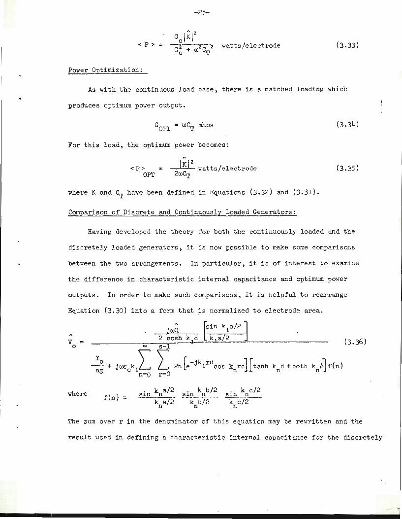
< p > = watts /electrode (3.33)

Power Optimization:

As with the continuous load case, there is a matched loading which

produces optimum power output.

(3.34)

For this load, the optimum power becomes:

" <P> .

. OPT IKI 2

~~-=+--watts/electrode 2wCT

(3.35)

where K and CT have been defined in Equations (3.32) and (3.31).

Comparison of Discrete and Continuously Loaded Generators:

Having developed the theory for both the continuously loaded and the

discretely loaded generators, it is now possible to make some comparisons

between the two arrangements. In particular, it is of interest to ex~~ine

the difference in characteristic internal capacitance and optimum power

outputs. In order to make such comparisons, it is helpful to rearrange

Equation (3.30) into a form that is normalized to electrode area.

v 0 =

where f(n) =

sin kna/2

k a/2 n

. k b/2 s~n n

k b/2 n

. k c/2 s~n n k c/2 .n

(3 0 36)

The 3um over r in the denominator of this equation may be rewritten and t~e

result used in defining a ~haracte ristic internal capacitance for the discretely

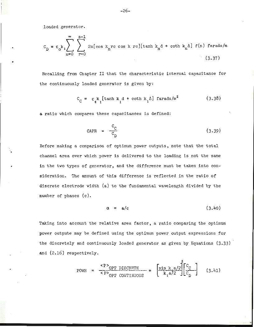
-26-

loaded generator.

oo s-1

CD= E0k

1L L 2n[cos knrc cos k rc][tanh knd + coth kn6] f(n) farads/m

n=O r=O (3.37) ..

Recalling from Chapter II that the characteristic internal capacitance for

the continuously loaded generator is given by:

E k [tanh k d + coth k 6] farads/m 2

0 1 1 1 (3.38)

a ratio which compares these capacitances is defined:

CAPR = (3.39)

Before making a comparison of optimum power outputs, note that the total

'· channel area over which power is delivered to the loading is not the same

in the two types of generator, and the difference must be taken into con-

sideration. The amount of this difference is reflected in the ratio of

discrete electrode width (a) to the fundamental wavelength divided by the

number of phases (c).

ex = a/c (3.40)

Taking into account the relative area factor, a ratio comparing the optimum

power outpute may be defined using the optimum power output expressions for

the discretely and continuously loaded generator as given by Equations (3.33)

and (2.16) respectively.

PO\ffi = < p > OPI' DISCRETE

< P> OPI' CONTINUOUS (3.41) =

-27-

Due to the double sums involved in the above ratios, the computer was

used to make s 'ample calculations for curve plottin.g, a.11d the programs

designed and employed fer this purpose are contained in Appendix C.

Curves 3.1 and 3.2 demonstrate how the ratios : expressed in Eq. (3.39)

and Eq. (3.41) vary according to the number of phases used per wavelength

and the degree to which the discrete electrodes occupy the channel inter­

facial area. It should be emphasized that these curves are only as good

as the model frnm which they were obtained. For this reason, they should

not be expected to give valid results at the extremes of the ranges.

The range of a studied is felt to correspond to that range over which

the discrete generator model is valid. From curve 3.1, note that CAPR is

a maximum overall s for a= .5, and decreases symmetrically for a greater

or less than this value.

Curve 3.2 demonstrates the effects of a and s on output power. It

appears from these curves that large a and s would be the most desirable

arrangement. 1be power ratio goes asymptotically to a as s is increased

to large values and is always less than a due to the area difference

between discrete and continuous loading. However, as a · and s are increased,

the spacing gets very small and electric field breakdown strength becomes

of critical importance.

Using curve 3.2, one is led to make the optimistic judgment that dis­

cretely loade j charge-constrained generators compare very favorably with

continuously loaded ones on the basis of power output. An energy conver­

sion efficiency which quantifies the degree to which the maximum amount of

power available is removed from a discretely loaded generator as a function

of a and s is displayed on curve 3.3. The information used to plot this

- 28-

curve is contained in curve 3 . 2 a~d is not a reflection of me chanical to

electrical conversion efficiency. All generators conside red are assumed

to be 100 per cent efficient in this regard, as no losses have been included

in the model.

Experiments on an actual generator are now in order so that the theory

on which the preceding calculations are based may be verified .

1.0

.9

. 8 I

tx; ~ • 7 u

I . 6

. 5

. 4

. 3

. 2

. 1

CAPR -CContinuous

CDiscrete

---------------------------

a.= .5 - -

a.=·3~ -

a=

Asymptote:

0 2 4 6 8 10 12 14 16 18 20 22 24 26

- s -

Curve 3.1

k d = .18 1

k !:.. = 50 1

a = Electrode width

sc = Wavelength

s = Number of phases

a. = a/c

28 30 32 34 36 38 4o

I [\)

"' I

1. 0

o9

o8

o7

o6

0 5 I

~ oh 0 p..,

I

o3

. 2

ol

0

< P> oprr DI SCRETE

POWR = < p > OPT CONTINUOUS

Asymptote ~ - - _,.-

k d = .18 1

k 6 = 50 1

a = Electrode width

sc = Wavelength

s = Numbe r of phases

CL = a/c

--- --------------------------------------------------

CL =

------------- --------------------------------------CL = o 5

--------------------------------------------------CL = . 3

2 4 6 8 10 12 14 16 18 20 22 24 26 28 30 32 34 36 38 40

s

Curve 3.2

I w 0 I

I

» ()

~ <1>

•r-i ()

•r-i c.-. c.-. ~

~ 0

•r-i

~ 1:-l

·r-i rl •r-i ~ ;:::,

!-< 0 ~ rj !-< <1> ~ Q)

0

100

95

90

85

80

75

70

65

60

55

50

..

100%

----------------- --- -- ---- -- --- -- --- -- ----------- -- -- -- --- ---

k d = .18 1

k 1::. = 50 l

a = Elect rode wi dth

sc = Wavelength

s = Numbe r of phases

a = a/c

Asymptote:

0 2 4 6 8 10 12 14 16 18 20 22 24 26 28 30 32 36 38 40

s

Curve 3.3

I w f-' I

-32-

CHAPTER IV

EXPERIMENTAL COMPARISON l,.JITH THEORETICAL PREDICTIONS

Introduction:

In Chapter III, a general theory was developed for determining the

loadigg characteristics of the charge-constrained synchronous generator.

Modifications to this theory, to account for the geofletry of the experi-

mental generator, have been developed and are presented in Appendix A.

It is now possible to present a theory which applies strictly to the

laboratory generator and to make predictions concerning its output

characteristics.

From Equation (3.30), the output voltage for any electrode in the

uniform loading situation is: ·

where:

v 0 =

yo - + jw g

D 00

f(n)

n=O

k a/2 sin knb/2 sin knc/2 f(n) = cos knrc sin n

(4.1)

(4.2)

In Appendix A, the modifications for D, Cn c

and C are developed, taking nL

into account the char act er of the actual channel. The result for the source

term, using (A.ll), was:

" D =

The modified capacitance for t he channel is:

£ k [e: f + tanh k d) o n r 1 n [1 + £ f t anh knd]

r 1

(4.3)

(A.lO)

r

t

•

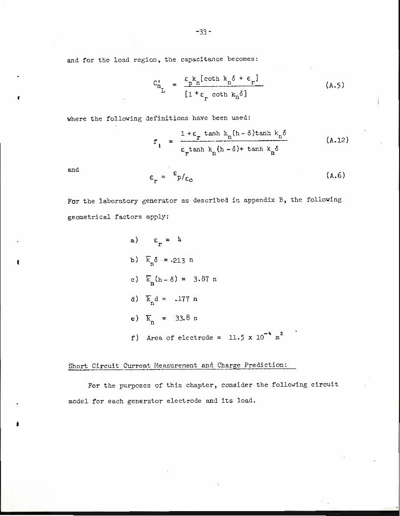
-33-

and for the load region, the capacitance becomes:

C' n L

= £ k [coth k o + £ ] p n n r

[1 + £r coth kno]

where the following definitions have been used:

1 + £ tanh k (h- o )tanh k o r n n =

£ tanh k (h - o )+ tanh k o r n n

and

(A. 5)

(A.l2)

(A.6)

For the laboratory generator as described in appendix B, the following

geometrical factors apply:

a)

b)

c)

d)

e)

f)

£ = 4 r

k o · = ·213 n n

k (h- 0) = n 3.87 n

k d = .177 n n

K" = 33.8 n n

Area of electrode -It 2 = 11.5 X 10 m

Short Circuit Current Measurement and Charge Prediction:

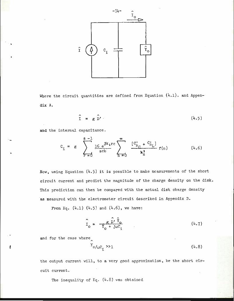
For the purposes of this chapter, consider the following circuit

model for each generator electrode and its load •

\ '-~ ..

' ..

(

" I c. ].

-34- A

_..._ --

Where the circuit quantities are defined from Equation (4.1). and Appen-

dix A.

" " I = g D'

and the internal capacitance.

c. = g ].

(4.5)

(4.6)

Now, using Equation (4.5) it is possible to make measurements of the short

circuit current and predict the magnitude of the charge density on the disk.

This prediction can then be compared with the actual disk charge density

as measured with the electromete r circuit described in Appendix B.

From Eq. (4.1) (4.5 ) and (4.6), we have:

I = 0

and for the case where

" " g D' Yo

yo + jwCi (4.7)

(4.8)

the output current will , to a very good approximation, be the short cir-

cuit current .

The inequal ity of Eq. (4. 8 ) •ras obtained

r -

-35-

on the experimental generator by loading with a pure resistance that

gave: Y = 2 x 10- 7 ohms

0 (4.9)

It will become clear later that this loading does indeed satisfy the

condition i mposed by Eq. (4.8).

To determine the relationship between the short circuit current and

the surface charge density, recall:

A

III = k1

cosh k d[l + e: f tanh k d] 1 r 1

(4.10)

Since the ele ctrode current is given by the integral of the current den-

sity over the area of the electrode, and since the dimensions of the

electrodes vary due to the cylindrical arrangement, it is appropriate to

let

g = Area of Electrode a

(4.11)

where a is the electrode width over which the integr ation (3.17) was

carried out.

Using the nume rical values presented in Eq. (4.4), a relationship

for predicting the disk surface char ge density from the source (i.e.,

short circuit) current is obtained . Evaluation yields:

A A

jQj = 3.4llrl coul/m 2 (4.12)

The following short t able compar es the magnitude of the surface charge

density as pred~cted from the short-circuit current and that measured

with the electrometer to demonstrate the validity of equa-

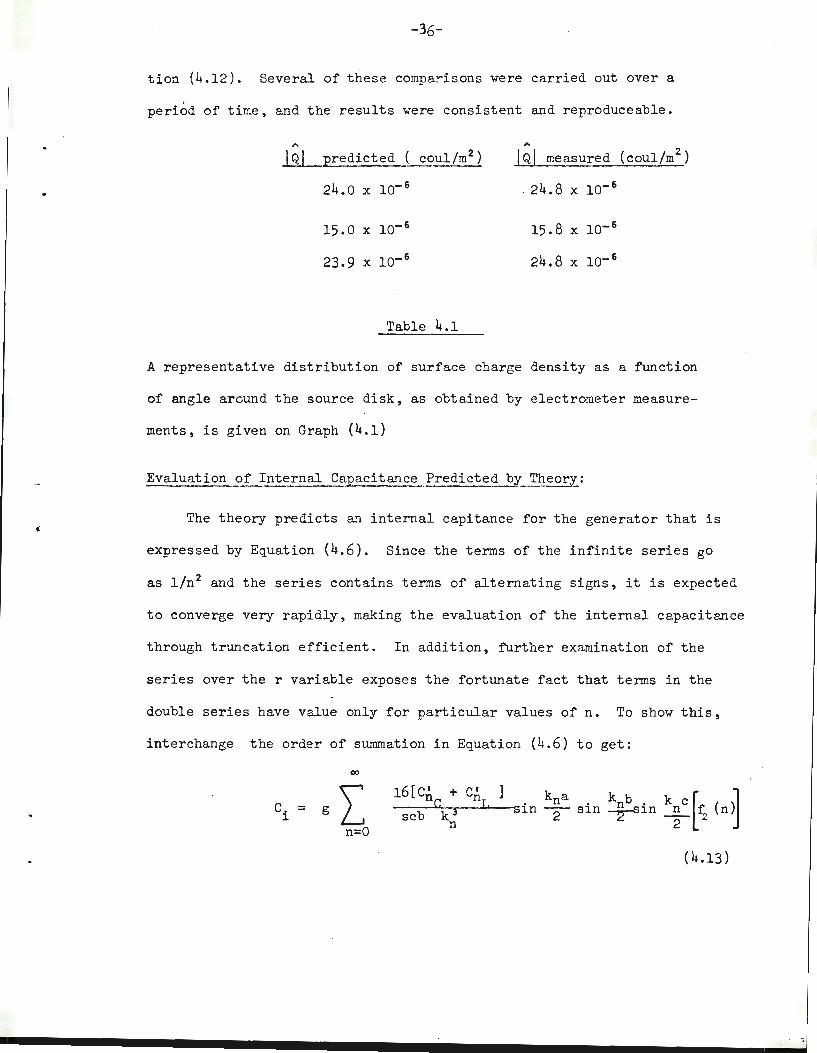
-36-

tion (4.12). Several of these comparisons were carried out over a

period of time, and the results were consistent and reproduceable.

" " IQI predicted ( coul/m 2) JQI measured (coul/m 2

)

24.0 X 10- 6

Table 4.1

. 24.8 X 10- 6

15.8 X 10- 6

24.8 X 10- 6

A representative distribution of surface charge density as a function

of angle arcund the source disk, as obtained by electrometer measure-

ments, is given on Graph (4.1)

Evaluation of Internal Capacitance Predicted by Theory:

The theory predicts an internal capitance for the generator that is

expressed by Equation (4.6). Since the terms of the infinite series go

as l/n2 and the series contains terms of alternating signs, it is expected

to converge very rapidly, making the evaluation of the internal capacitance

through truncation efficient. In addition, further examination of the

series over the r variable exposes the fortunate fact that terms in the

double series have value only for particular values of n. To show this,

interchange the order of summation in Equation (4.6) to get:

go

L 16[C~ + C' c. = g c nr. ~ scb k3

n=O n

(4.13)

..

-37-

where s-1 j2n(n+l)r -j2n(n-l)r ) e s + e s ~ --=---~2----'----- (4.14)

In Eq. (4.14) the exponential form of cos k rc and the definition of n

Eq. (3.4) have been used.

Examination of Eq. (4.14) reveals:

3 n=l; n+l n-1 1,2,3 --= m· --= m m = ...... s ' s

f (n) = (4.15)

0 otherwise o:: of s roots of l)

This of course greatly facilitates the evaluation of the internal capa-

citance predicted by the theory. For the case s = 6:

(X)

__.§£_ L[c.' + c I ] k a k b k c nc nL sin sin sin c. = k3 n n n

1 cb il 2 2 2

n=O (4.16)

n = 1,5,7,11,13,17,19 ----

Using the physical characteristics of the generator as presented in

Appendix B and truncating the infinite series, one obtains for the inter-

nal capacitance associated with each electrode, as predicted by the theory:

c. = 1

-12 4.7 x 10 farads

Sources of · C a~acitance Not Accounted for in Theory:

The theory as modified in Appendix A does not fully account for all

the capacitance that characte rizes the generator. The most significant

source of capacitance unaccounted for in the theory has to do with the

finite dimension of the electrodes in the vertical coordinate and the

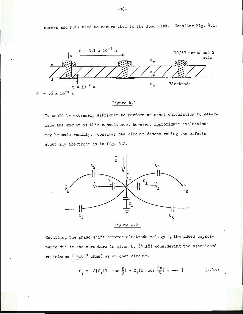
-38-

screws and nuts used to secure them to the load disk.

-2 c = 3.1 x 10 m

t = 10- 3 m

o = .6 x 10-2 m

Figure 4.1

Consider Fig. 4.1.

10/32 screw and 2 nuts

Electrode

It would be extremely difficult to perform an exact calculation to deter-

mine the amount of this capacitance; however, approximate evaluations

may be made readily. Consider the circuit demonstrating the effects

about any electrode as in Fig. 4.2.

Figure 4.2

Recalling the phase shift between electrode voltages, the added capaci-

tance due to the structure is given by (4.18) considering the associated

resistance ( ~10 10 ohms) as an open circuit.

(4.18)

- r

•

-39-

Using the impedance bridge , it was possible to get an experimental

measurement of the capacitance involved in Equation (4.18)

Using these results:

c 1

c 2

c3

c It

c s

= = =

"' '"'

=

1.5 pf

-75 pf

.25 pf

0

12 4.8 X 10- farads (4.19)

Unfortunately this capacitance is approximately equal in magnitude

to that predicted by the theory as inherent to the generator. However,

any st::cucture that might be devised to hold the electrodes would have

some capacitance associated with it. With both the intern~ and struc-

tural capacitances so small, the result of any attempt . to further reduce

them would be difficult to detect. The structure capacitance wa? inclu-

ded in the equivalent generator circuit used to predict output. This

total capacitance was considered as the characteristic capacitance of each

electrode.

Prediction of Matching Load

= c. + c l. s

-12 = 9.5 x 10 farads

(4.20)

The experimental generator contains five wavelengths of electrodes

with six (6) electrodes per wavelength, as is described in Appendix B.

To avoid the problems involved in loading each electrode as a separate

source, the experiments were conducted with electrode outpu~of the same

phase connected in parallel. This required the attachment of only six

-40-

loads to obt ain ~haract eri z ing output data. The modifications to the

generator equivalent circuit are obvious:

"' "' (a) I -+ 5 I

(b) CT -+ 5 CT (4.21)

"' " (c) y -+ 5 y

0 0

Using the generator so configured, that is, like phase assembled in paral-

lel, it was possible to predict the loading for maximum power output

using the results of Chapter III and Equation (4.20).

(a) y = 5 w CT mhos (4.22) LOPI'

and for w=377 rad/sec

(b) y = 17.9 X 10- -9 mhos LOPI'

and t 6

(c) R = 56 X 10 ohms LOPI'

This represents the loading that is predict~d by the theory for the

generator to produce maxi mum power with five electrodes of the same phase

wired in parallel. On a per-electrode basis, if each electrode was loaded

individually, the required loading is as predicted in Equation (4.21):

280 x 106 ohms (4.23)

The effect of parallel operation in dete rmining the matched load condi-

tion increases t he flexibility in appl ication of such generators.

Experi mental Dete rmi nat ion of a Matched Load:

To obtai n t he output dat a f rom t he experimental gener ator, for the

purpose of i dentifyi ng the actual internal capacitance, it was wire d in

parallel, as described in t he pr evious section .

-41-

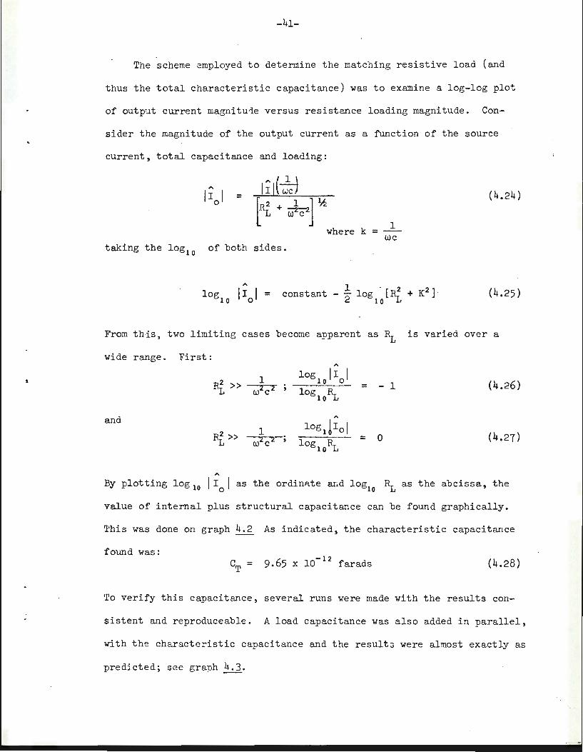
The scheme employed to determine the matching resistive load (and

thus the total characteristic capacitance) was to examine a log-log plot

of output current magnitu1e versus resistance loading magnitude . Con-

sider the magnitude of the output current as a function of the source

current, total capacitance and loading:

" II I 0

=

taking the log10

of both sides.

where k = 1 we

(4.24)

" log II I =

10 0 constant - ! log - [R2 + K2] ·

2 10 L (4.25)

From this, two limiting cases become apparent as R1 is varied over a

wide range. First: "'

1 log II I R2 10 0

- 1 (4.26) >> ~T = L log R1 10

and "'

R2 >> 1 log1biol 0 (4.27) ~-; = L log ~

10

" By plotting log 10 I I I as the ordinRte aLd log R1 as the abcissa, the 0 10

value of internal plus structural capacit~~ce can be found graphically.

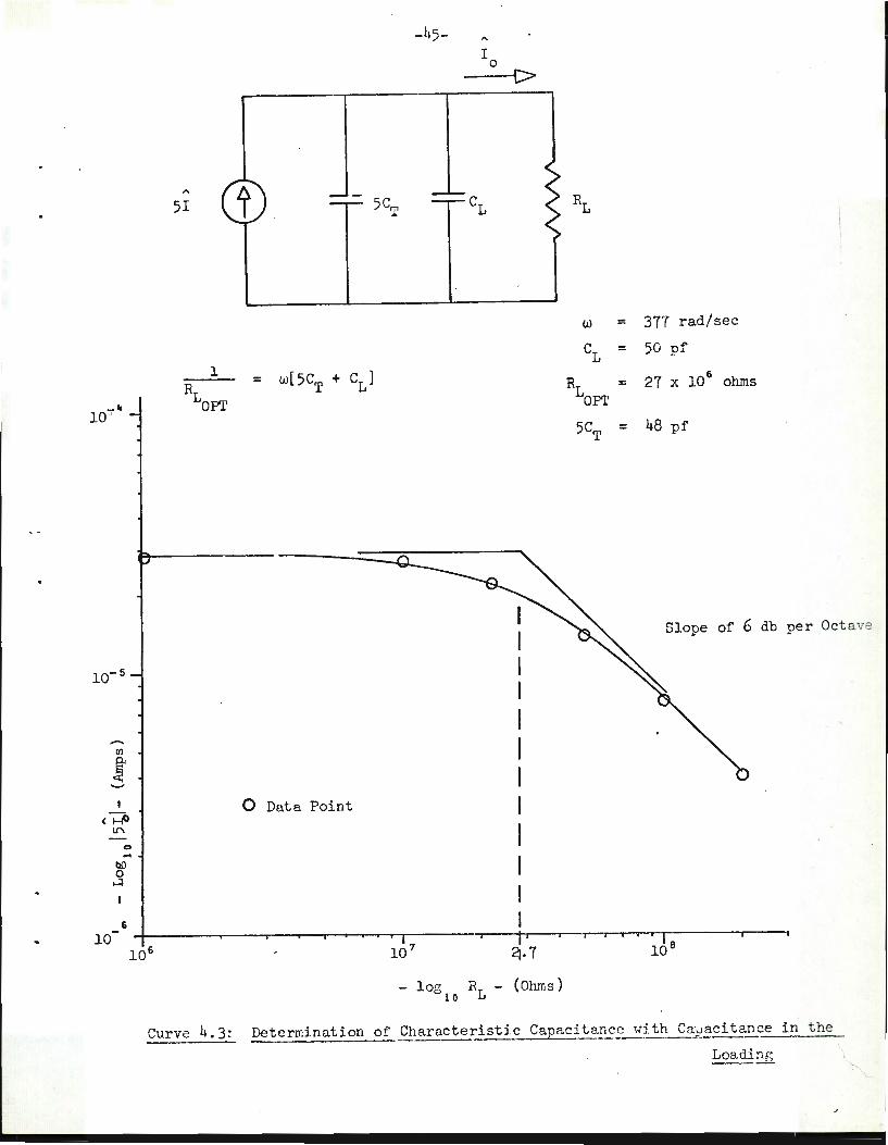
This was done on graph 4.2 As indicated, the characteristic capacitance

found vras: CT = 9.65 x 10- 12 farads (4.28)

•ro verify this capacitance, several runs vrere made with the results con-

sistent and r eproduceable. A load capacitance was also added in parallel,

with the characteristic capacitance and the result3 were almost exactly as

predicted; see graph 4.3. - --

(

-42-

The power output curve as a function of loading was also calculated

and plotted on graph 4.4. Note that the maximum power output occurs at

matched loading .

Discussion of Results:

The validity of the theoretical model assumed to characterize the

charge-constrained generator has been demonstrated in the previous sec­

tions. In particular, the magnitude of the equivalent current source may

be accurately predicted by the theory for a known surface charge density.

The experiments have shown the actual internal capacitance to be

approximately twice that which would be predicted by the theory alone.

However, this predicted capacitance did not include that capacitance

associated with the structure of the generator. When this extra capaci­

tance had been estimated and included as part of the characteristic in­

ternal capacitance of the generator, then the theoretical prediction

accurately matched the actual generator characteristics. However, it is

felt that the most accurate method of characterizing a generator in terms

of equivalent circuit elements, for application, would be to obtain a plot

of equation (4.24). The theory serves the purpose of providing an approxi­

mation of the capacitance for design purposes, but due to the structure the

actual capacitance would _have to be determined after construction. This

does not dif~er from the procedure followed for designing and characteri­

zing magnetic field machines.

Cll)

1•1·

I 0 rl

>< ~

Ul .0 s 0 rl ;::j 0 u ~

I

bO !=:

•rl 'd ro I]) ~

H 11! +' (!) p d H +' (.) Q)

rl ;:-.J

...

1.5

1.0

.5

0

-.5

-1.

-1.5

Q =

if

Electrometer Reading

Area of Probe

r4~0 ~ 't 90

Curve 4.1: Disk Charge Distribution

coul/m2 _.. 2 Area of probe = 5.25 x 10 m

t 18~t t 2;5° t 27~~ ~ 3~5° t I

~3~ 0 I Q .t::' .. lAl I

360°

0 = Data Point

Q = Angular Position on Disk

'

10 _ ..

0 ...

R

5I

1 5 CT =

1oPT

0 Data Point

- 44-

I 0

--t>

w R . 10PT

5CT

= =

=

- Log R1

- (Ohms ) 10

Curve 4 . 2

377 r ad/ s e c

56 X 106

ohms

47. 5 pf

Slope of 6 db pe r

octave

_ .. 10 "

I

< .....,<~ ll"\

0 ... bO 0

...:I

6

51

1 w[5CT + c1 ] = R LOPI'

0 Data Point

- 45-

10 7

I 0

---t>

- l og R1 - (Ohms ) 1 0

-R

w = 377 rad/sec

CL = 50 pf

27 X 10 6 ohms = LOPI'

5CT = 48 -pf

Slope of 6 db per Oct ave

Curve 4.3 : Dete rmination of Characterist ic Caoaci t ance vith Ca~acitan ce in the

Loading_

'- -20

19

15

10

0

0 I

56

-46-

Powe r Output per 5 Elect r odes Vs Load R1

51

< p > = Powe r Delive r ed to R1 "' 5lrl = 40 X 10- Amps

5 CT = 47.5 pf

R = 56 Hegohms 1oPT

< P >0PT= 19 Mi lliwat t s per 5 Electrodes

100

6. Data Point

200

- R1 - (Megohms )

Curve 4. 4

300

-47-

CHAPTER V

Conclusion:

The application of charge-constrained synchronous generators in

the production of large amounts of electrical power is to a great extent

dependent on the feasibility of power removal with a finite number of

discrete electrodes. That is, such generators must have output terminals

with a finite number of phases through which they can deliver power.

Otherwise, they are strictly limited to continuum type loading.

In Chapter III a discretely loaded generator with an arbitrary num- ·

ber of phases was analyzed. By modeling the potential distribution between

adjacent electrodes as a linear function, it was possible to obtain a ter­

minal pair representation for each electrode's output. The equivalent

circuit for each electrode was shown to be accurately represented by a

current source in parallel with a characteristic internal capacitance.

It was then demonstrated in Chapter IV that the magnitudes of both of

these equivalent lumped elements was accurately predicted by the theore­

tical model. The need for a means of obtaining an accurate estimation of

that part of the internal capacitance due to the physical structure of

the load electrodes was demonstrated in the experimental section of this

research.

Of prime interest in the use of discretely loaded generators is the

amount of power din1inution that occurs comparative to the case of contin­

uous loading. It has been shown that this penalty need not be severe if

the electrode spacing and number of phases are carefully chosen. With the

power output per fund&~ental wavelength of channel length directly proper-

'~ :

-48-

tional to the electrode area it becomes important to make the inter-

electrode spacing as small as field breakdown strength -.rill allow.

It is this factor which has the most significant effect in reducing

power output when using discrete vice continuous loading.

It has been shown theoretically that a discretely loaded generator

can perform efficiently as an energy converter. However, in this regard

there are several unanswered questions which may serve as the basis for

further investigations in the development of a practical system. The

ability of such a generator to run self-excited, from start-up, is of

obvious interest. Mechanical energy storage schemes have been propose~J2) to accomplish just this, but is is yet to be demonstrated on an actual

device. Questionable is the feasibility of constructing a generator with

rotational speeds in excess of 30,000 rpm and providing it with a high

vacuum environment so that high electric field intensities may be sup-

ported. And lastly is the obvious problem as yet unconsidered, of

adapting a six-phase plus generator to provide power for a three-phase

world. Needed for this is a very efficient, lightweight phase transfor-

mer or system of capacitors which would combine the phases.

APPENDIX

l

-49-

APPENDIX A

Modification to Theory for Experimental Generator

Introduction

For the generator built to provide experimental verification

of the theoretical model considered in Chapter III, it was necessary to

make some changes to the load and channel arrangements. Practical con-

sideration dictated that the channel be asymmetrically loaded and that

plexiglas disks be used to support the electrodes and to carry the

exciting charge distribution. These changes do affect the field dis-

tribution, and therefore must be reflected in any theory applied to

predict output for this particular generator. Conceptually there are

no changes; however, the equivalent source and internal capacitance-

lumped elements predicted in Chapter III must be modified. A cross-

sectional view of the laboratory generator is given in Figure A.l,

and demonstrates these changes.

y

h

€: 0

w m

C..l:--- Rotating

• • d + 6 T·n_ v~::L-L-.L..LJ.I~~-11-..JLJ.....t....l..~'-<-L_._.::!;;A~ V I I I II

shaft

Plexiglas disk supporting load­ing electrodes

Plexiglas disk with surface charge density

Ground plane

Figure A.l

y

-50-

Appendix A

Since the voltage distribution along the electrodes is as sume d known,

it is efficient to consider the modifications to the theory in two steps.

First, consider the effect of the plexiglas l aye r above the electrodes on

the characterist ic capacitance of the load CnL' as defined in Chapte r III.

Secondly, consider t he effect of the plexiglas l aye r below the electrodes

and the asymmetric loading on the source term JS, and characteristic

channel capacitance cn.c • both as defined in Chapter III. 'l'hese modified

equivalent lumped elements should be used in msking theoretical predic-

tions for the experimental generator.

Effect of Plex i gl as Layer A~?ve Electrodes

'!'he theoretical developments for this and the next section are car-

ried out using techni ques i dentical to those used in Chapter III. Any

question conce r n ing procedure should be referred to this chapte r, as it

is not felt to be necessary to go into the same amount of detail in the

expositions of this appendix.

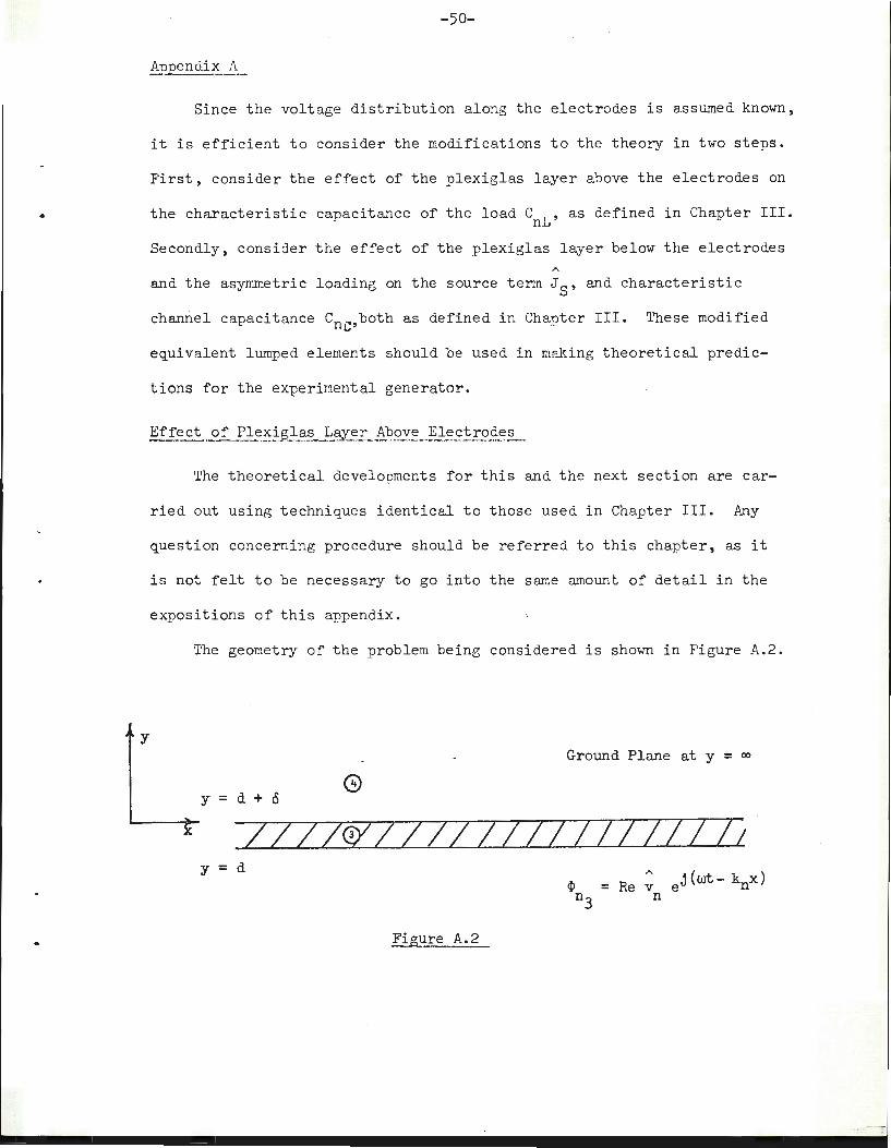
The geometry of the problem beins conside red is shown in Figure A.2.

Ground Plane at y = co

y = d + 0

ZZZZWZZZZIII/ZZZZZZZI y = d

Figure A.2

= Re v n

i

-51-

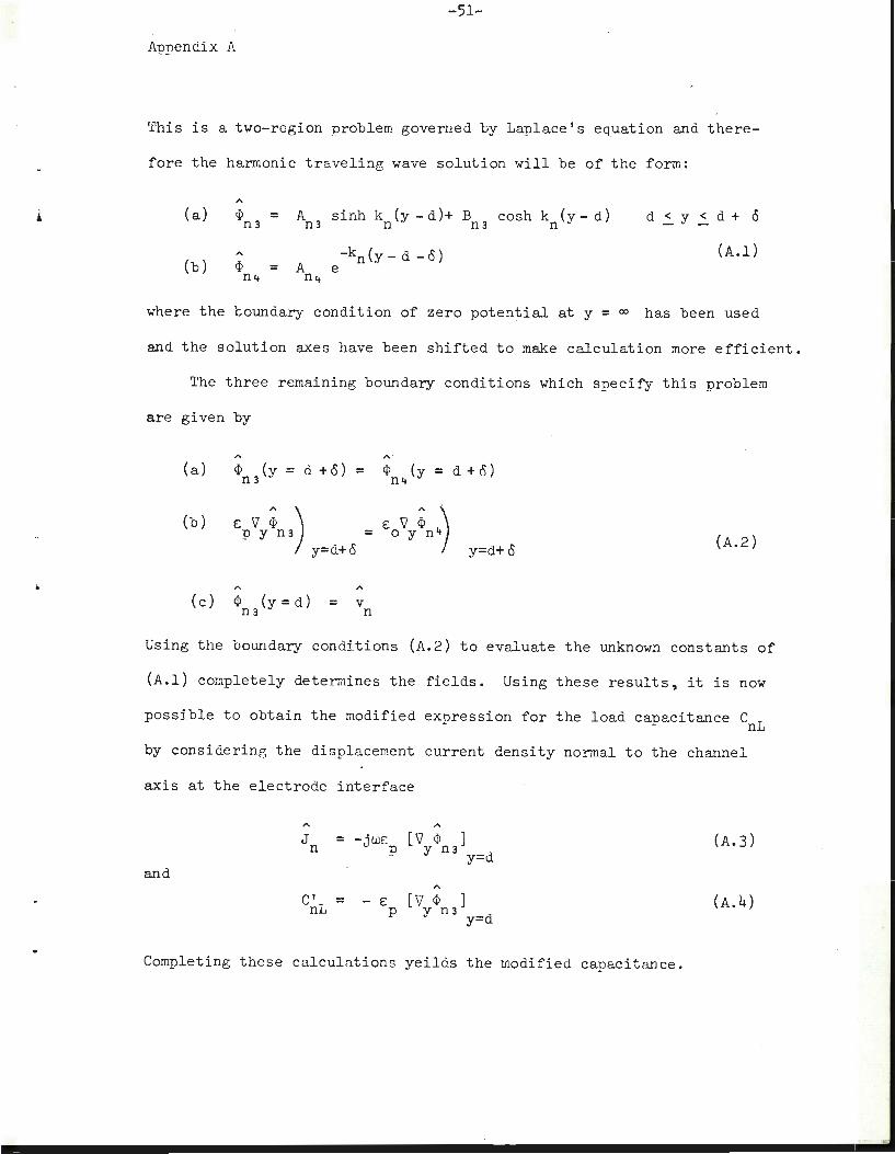
Appendi x A

This is a two-region problem governed by Laplace's equation and there-

fore the harmonic traveling wave solution will be of the form:

(a) .p = A sinh k (y- d)+ B cosh k (y- d) d::._y::._ d+ 0 n3 n3 n · n3 n

-kn(Y- d-o) (A.l) (b) ¢ = A e nLt n4

where the toundary condition of .zero potential at y = oo has been used

and the solution axes have been shifted to make calculation more efficient.

The three remaining boundary conditions which specify this problem

are given by

A ·

(a) ¢ (y = d + 0) = .p (y = d + 0) n3 nLt

(b) e: 'V¢) e:'V ¢4)' p y n3 = o y n y=d+o y=d+o (A.2)

(c) .p (y=d) = v n3 n

Using the boundary conditions (A.2) to evaluate the unknown constru1ts of

(A.l) completely determines the fields. Using these results, it is now

possible to obtain the modified expression for the load capacitance CnL

by considering the displacement current density normal to the channel

axis at the electrode interface

J = -jws ['Vy.Pn3] n p y=d

(A. 3)

and A

C' = E: [ 'V Q ] nL p y n3 y=d (A. 4)

Completing t hese calculations yeilds t he modified capacitance.

Appendix A

whe r e

-52-

e: k [ coth k o + e: ] C' = p n n r

nL [ 1 + e: coth k o] r n

2 farads/m

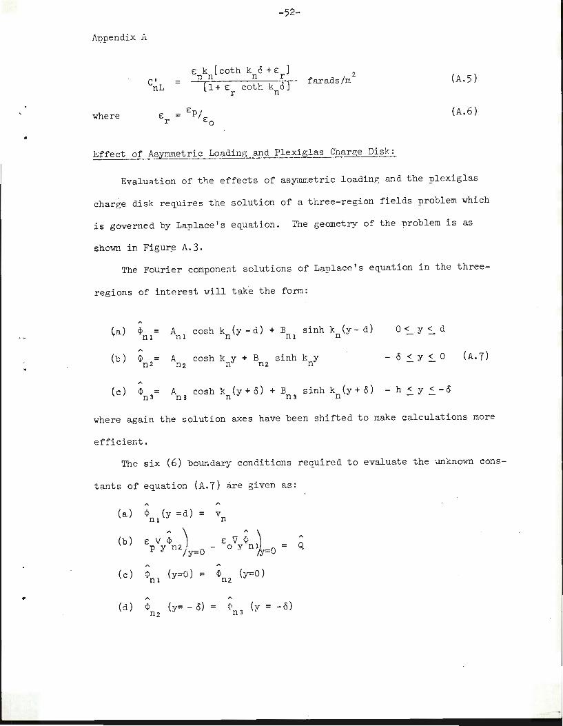
Ef fe ct of A~etric Loading and Plexiglas Charge Dis~~

(A. 5 )

(A .6 )

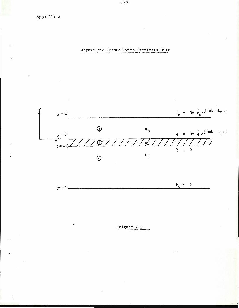
Evaluation of the effects of asyillmetric loading and the plexiglas

charge disk requires the s ol ut i on of a three- region fields probl em which

is gove r ned by Laplace ' s equat ion. The geometry of the problem i s as

shown i n Figur~ A. 3.

The Fourier component solutions of La~lace's equation i n the th r ee-

r egions of i nterest vill take the form :

" ( a ) ¢ = A cosh k (y - d ) + B sinh kn( y - d ) 0 -:._y~ d

n l n 1 n nl

" (b) ¢ = A cosh k y + B s i nh k y - 0 :_y ~ 0 (A. 7 )

n2 n 2 n n 2 n

(c) ¢ = n3 A n3 cosh k (y + o ) + B n n3

sinh k (y + o ) n - h .:s_ y.::_ - o

where again the sol ut i on axes have been shi fted to make calculat i ons more

efficient .

The six (6) boundary condit i ons r equired t o evaluate the unknown cons -

t ant s of equation (A .7 ) are gi ven as :

" " (a) ¢ (y =d ) = v

nl n

(b) e: 17 ¢ ) p y n2 / y=O

e: 17 ¢ " ~ - o y n 1 =O = Q

" (c) ¢ (y=O) = ¢ (y=O )

n1 n 2

( d ) <P (y= - o) = cp (y= - o) n2 n 3

-53-

Appendix A

Asymmetric Channel with Plexiglas Disk

..

= Re v" ej (wt- knx) y=d ~ n

------------------------------------------------~------~~--

Q = Re Q e j ( wt - k1 x)

<P = 0 y=-h--------------------------~--------------U-----------

Figure A.3

-54-

Appendix A

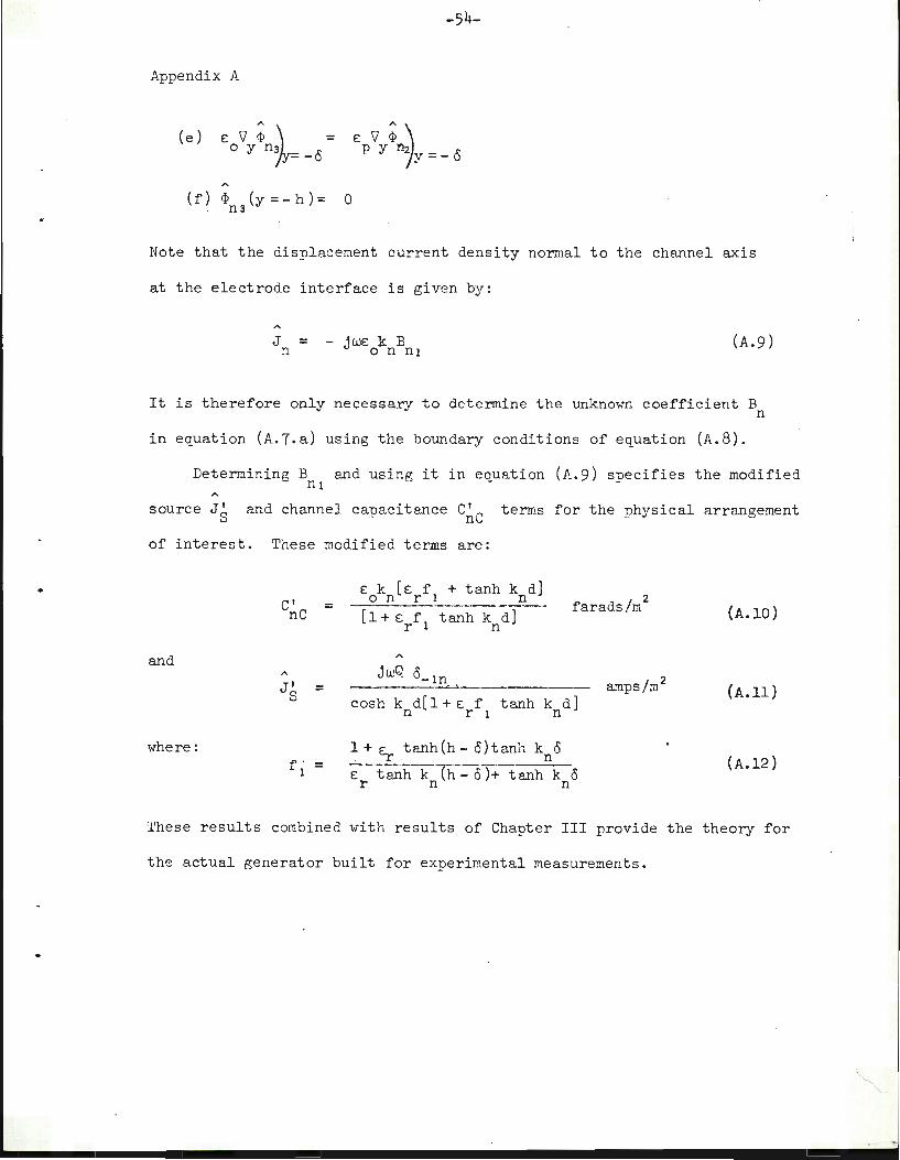
"' A ~ (e) E: 'i7 ¢ ~ = E: 'i7 ¢

o y n3 = _6 P n2 - y y=-6

"' (f) ¢ (y=-h)= 0 n3

Note that the displacement current density normal to the channel axis

at the electrode interface is given by:

J = - jwe: k B n o n n1 (A . 9)

It is therefore only necessary to determine the unknown coefficient B n

in equation (A.7.a) using the boundary conditions of equation (A.8).

Determining B and using it in equation (A.9) specifies the modified nl

source JS and channel capacitance C~C terms for the physical arrangement

of interest. These modified terms are:

and

where:

C' = nC

J ' = s

f' = l

e: k [ e: f + tanh k d ) o n r 1 n [1+ e: f

1 tanh k d) r n

jwQ 6-ln - .

2 farads/m

amps/m 2

cosh k d[ 1 + e: f n r 1 t anh k d) n

1 + ~ tanh(h- o)tanh kno

z- tanh k lh-- 0 ) + tanh k 0 r n n

(A. lO)

(A.ll)

(A.l2)

These results combined with results of Chapter III provide the theory for

the actual generator built for experimental measurements .

-55-

APPENDIX B

Experimental Generator:

General Generator Arrangement:

An asymmetrically loaded, charge-constrained synchronous generator

was designed and built as part of this thesis project so as to provide

verification of theoretical results. A sketch of the device built is

presented in figure B.l.

The physical measurements of this generator are given below and should

be used in any application of theory to predict output. Note that a mean

wavelength, and therefore mean wavenumber, is used to characterize the

load section. This is necessary since the wavelengths at the inside and

outside tips of the load electrodes are different, due to the cylindrical

geometry. Since the theory considers a rectangular channel this consti-

tutes an approximation; however, the results as shown in Chapter IV indi-

cate that it is a good one.

I = 18.6 X 10-2 m 1

k = 1

33.8 m-1

0 = ,6 X 10- 2 m

-2 d = .5 x 10 m

(h- 0) = 10.9 X 10 -2 m

A 11.5 10-lt 2 = X m electrode

a/c = .61

Q) = 60 cps e

w = 10 cps m

e: = 4.0 r

8.854 -12 e: = x 10 farad/m 0

-5~-

Appendix B

Plexiglas was chosen as the material to be used for the structural sup-

port of the load electrodes because of its inherent attributes such as

' easy workability and transparency and its electrical properties are known.

The plexiglas ~as chosen for the charge disk material principally for its

extremely long characteristic relaxation time for bulk free charge.

Charges placed on the disk by rotating it through the corona exciter sec-

tion remain in place long enough to easily complete a full set of experi-

mental measurements. The charge disk can be fully energized in less than

10 sec. and then the corona section may be turned off to eliminate noise

in the electrode output signals.

In order that the corona exciting field would be in synchronism with

the charge wave established on the disk, it was required that disk rota-

tional frequency be diviS.ible into the exciting voltage frequency an

integer number of times. For the laboratory generator:

w 10 cps mechanical

welectrical 60 HZ = -- = 6

This establishes six wavelengths of charge distribution around the peri-

phery of the disk. The disk speed was obtained by using an 1800 rpm

synchronous motor driving the shaft with a toothed, flexible belt and a

set of 3:1 speed-reducing pulleys. With both the motor and corona being

driven from the same electrical mains, the maintenance of synchronism was

, not a problem. Electrodes were arranged on the load disk at six electrodes

per wavelength of charge distribution. Although there were six full wave-

lengths of charge distribution about the load section circumference, only

1

'-''

-57-

Appendix B

five wavelengths of load electrodes were installed. The sixth wave­

length was left clear to accommodate the corona source.

Measurement of Disk Charge Density:

An important variable in describing the generator output is the

magnitude of the charge distribution wave on the disk. It is not pos­

sible to gat an accurate measure of this charge magnitude simply by

knowing the magnitude of the corona voltage. A direct measurement of

the distribution was obtained using a Kuthly Electrometer model 610B in

conjunction with a flat plate sensing proble of known area. The probe

was mo1L.'1ted in the location >There the corona source is set during the

disk charging cycle. Manually rotating the disk then puts the probe

under the influence of the charge, the magnitude being a function of

position.

The electrometer is a de instr1Lment which measures the charge by

integrating the current required to set up image charges for that charge

influencing its probe. For this reason, it was necessary to make the

rotation of the disk for charge distribution purposes extremely slow.

Using this scheme for charge measurement gave consistent, reproduceable

results which compared very well with theoretical predictions as shown

in Table 4 .1.

Pictures of the loading section with the electrodes loaded individ­

ually and in parallel· are given in Figure B.2. These pictures also show

the electrometer probe and corona source as they appear when mounted.

- 58-

>. m

g

l 14 .. I

8;2

Elect r ode Load Disk

Rl = 14.0 x 10- 2 m

_2 R = 21.5 X 10 m

2 •

IV = 6,0°

e = 6 . 1°

-2 a = l.Ox 10 m

1

-2 a = 2.15 x 10 m

2

g = 7,5 X 10 -2

m

w e l ectrical w = m 6

I . Charge Disk

Figure B. 1

-59-

(a)

View Showing Load Electrodes of the Same Phase Connected in Parallel.

Note Corona Source in Position in Foreground.

(b)

View Showing Each Electrode with Individual Resistive Loading. Note Elec­

trometer Char ge Measuring Probe in Position ip Foreground.

Figure B.2

-60-

APPENDIX,C

Computer Programs for Calculat ion:

The programs C.l and C.2 can be us ed to calculate the capacitance

ratio CAPR and power ratio POHR of Equations (3.39) and (3.41), respec-

tively. These ratios provide a comparison between discretely loaded and

continuous loaded, charge-constrained synchronous generators . If it is

desired to calculate both of these r at ios at the s ame time, the programs

may be efficiently combined to decrease the computer time required.

The require d inputs have, for the most part, been defined in Chapters

I and II.

KD = k d 1

KDELTA = k 6 1

ALPHA = a/c

s = number of phases

The integer M sets the upper limit on the summation over n. This series

· converges rapidly and six contributing terms provide v e ry good accuracy.

Recall from Chapter IV that terms in this sum are contributed only for:

n = 1;

The outputs are:

(n + 1) s

= integer ; (n- 1)

s = integer

H = capacitance for continuous generator

F = total value of double sum over s and n

K = CAPR or PO\..ffi (depending on program being used)

..

•

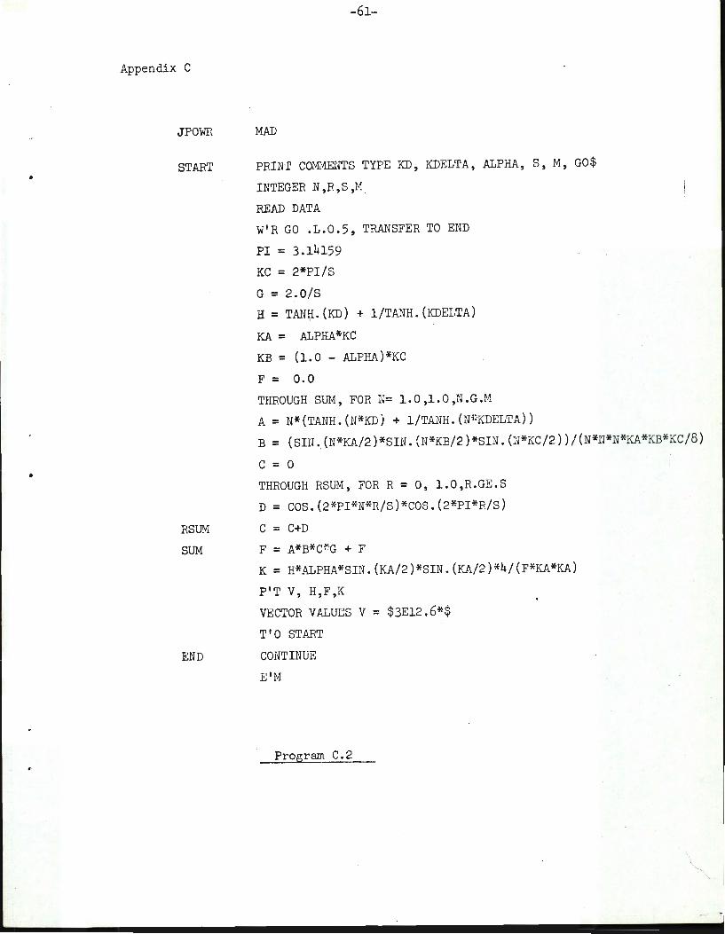
Appendix C

JPOWR

START

-61-

MAD

PRIN·r COMMENTS TYPE KD, KDELTA, ALPHA, S, M, GO$

INTEGER N,R,S,M

READ DATA

W'R GO .1.0.5, TRANSFER TO END

PI = 3.14159

KC = 2*PI/S

G = 2.0/S

H = TANH. (KD) + 1/TAJ-IH. (KDELTA)

KA = ALPHA *KC

KB = (1.0 - ALPHA)*KC

F = 0.0

THROUGH SUM, FOR N= l.O,l.O,N.G.M

A = N*(TANH. (N*KD) + 1/TANH. (N""KDELTA))

B = (SIH .. (N*KA/2 )*SIN. (N*KB/2 )*SIN. (N*KC/2)) /(N*f!*N*KA*KB*KC/8)

c = 0

THROUGH RSill~ , FOR R = 0, 1.0,R.GE.S

D = COS.(2*PI*N*R/S)*COS.(2*PI*R/S)

RS~ C = C+D

SUM F = A*B*C~·G + F

K = H*ALPHA*SIN.(KA/2)*SIN.(KA/2)*4/(F*KA*KA)

P'T V, H,F,K

VECTOR VALUES V = $3E12.6*$

T'O START

END CONTINUE

E'M

Program C.2

'-....

•

•

Appendix C

JCAPR

START

RSUM

SUM

-62-

MAD

PRINT COMiviENT$ TYPE KD, KDELTA, ALPHA, S,M,GO$

INTEGER N,R,S,M

READ DATA

W'R GO .1.0.5, TRANSFER TO END

PI = 3.14159

KC = 2*PI/S

G = 2.0/S

H = TANH. (KD) + 1/RANH. (KDELTA)

KA = ALPHA*KC

KB = (1.0 ~ ALPHA)*KC

F = 0.0

THROUGH SUM , FOR N= 1.0,1.0,N.G.M

A= N*(TANH.(N*KD) + 1/~ANH.(N*KDELTA))

B = (SIN.(N*KA/2)*SIN.(N*KB/2)*SIN.(N*KC/2))/(N*N*N*KA*KB*KC/8)

c = 0

THROUGH RSill~, FOR R=0,1.0,r.GE.S

D = COS.(2*PI*N*R/S)*COS.(2*PI*]/S)

C = C+D

F = A*B*C*G + F

K = H/F

P'T V, H,F,K

VECTOR VALUES V = $3E12.6*$

T'O START

END CONTINUE

E'M

R 1.033 + .283

Program C.1

I

:..63-

LIST OF REFERENCES

1. Woodson, H. H., and Melcher, J.R., Electromechanical Dynamics~ Chap­

ter 7, (in publication, John Wiley & Sons, Inc., New York, N.Y.

2. Trump, J. G., "Electrostatic Sources of Electric Power", Electrical

Engineering, June 1947.

3. Fitzgerald, A. E., and Kingsley, C. Jr., Electric Machinery, 2nd Ed.

(1961), McGraw-Hill Inc., New York, N.Y., p. 83.

4. Marks; A., Barreto, E., and Chu, C. K., "Charged Aerosol Energy Con­

verter", AIAA Journal _g_, No. 1, January 1964.

5. Devitt, E. B., "Power Density on An AC Charged Particle Generator",

Int. Ivtemorandum No. 140, Continuum Electromechanics Grou, MIT, 1968

6. Kahn, C., and Gourdine, M. C., "Electrogasdynamic Power Generation",

AIAA Journal _g_, No. 8, August 1964, pp. 1423-1427

7. Zipkin, M. A., and Edwards, R. N, ''Power Systems for Space Flight 11,

Academic Press, New York, N.Y. 1963, p. 917, and "Electrostatic

Power G~ne ration for Space" by Coenraads, C. , De.1holm A. S. , and

8.

9.

Lavelle, J. E. , and McCoy, F. J.

Van de Graaff, R. J., Trump, J. G., and Buechner, W. W. "Electrostatic

Generators for the Acceleration of Charged Particles", Reports on

Progress in Ph:ysics, Yol. XI, p. l (1948).

Gray, J. "Electrical Influence Machines", Whittaker and Co., London,

England, 1890.

10. Reeve, W. F., "Traveling-Wave SS!nchronous Electrohydrodynamic Power

Generation", S.M. Thesis, Dept. of Electrical Engineering, MIT,

(1967).

11. Herold, L., "Traveling- Wave Charged Particle Generation", S. M. Thesis,

Dept. of Electrical ~ngineering, MIT, (1967).

12. Melcher, J .R. "A Self-Exc ited Traveling-vlave Electrostatic and Elec­

trohydrodynamic Genera.tor", Int. Memorandum No. 135, Continuum

Elec-+; rome chanics Group , HIT, Dec. 1967

-64-

13. Regan, J. P., 11 A Cylindrical Charge-Constrained Synchronous Generator"

Internal Memo . No. 134, Continuum Electromechanics Group, HI'r,

l November 1967.

i

.•

r