1

Load Frequency Control in an AC

Microgrid

K Mahesh Dash (110EE0192)

Makhes Kumar Behera (110EE0120)

Vamsi Krishna Angajala (110EE0201)

Department of Electrical Engineering

National Institute of Technology, Rourkela

2

Load Frequency Control in an AC Microgrid

Bachelor of Technology in Electrical Engineering

SUBMITTED BY

K Mahesh Dash

ROLL NO - 110EE0192

Makhes Kumar Behera

ROLL NO-110EE0120

Vamsi Krishna Angajala

ROLL NO-110EE0201

Under supervision of

Prof. Susmita Das

Department of Electrical Engineering

National Institute of Technology, Rourkela

May 2014

3

DEPARTMENT OF ELECTRICAL ENGINEERING

NATIONAL INSTITUTE OF TECHNOLOGY, ROURKELA- 769 008

ODISHA, INDIA

CERTIFICATE

This is to certify that the thesis entitled “Load frequency control in an AC Microgrid”,

submitted by K Mahesh Dash (110EE0192), Makhes Kumar Behera (110EE0120) and

Vamsi Krishna Angajala (110EE0201) in partial fulfillment of the requirements for the

award of Bachelor of Technology in Electrical Engineering during session 2013-2014

at National Institute of Technology, Rourkela. A bonafide record of project work carried

out by them under my supervision and guidance.

Place: Rourkela

Dept. of Electrical Engineering Prof Susmita Das

National institute of Technology Professor

Rourkela-769008

4

ACKNOWLEDGEMENT

First and foremost, we are truly indebted and wish to express my gratitude to my

supervisor Professor Susmita Das for her inspiration, excellent guidance, continuing

encouragement and unwavering confidence and support during every stage of this

endeavor without which, it would not have been possible for us to complete this

undertaking successfully. We also thank her for her insightful comments and suggestions

which continually helped us to improve our understanding.

We express our deep gratitude to the members of Scrutiny Committee for their advice and

support. We are also very much obliged to the Head of the Department of Electrical

Engineering, NIT Rourkela Professor Anup Kumar Panda and Prof Sukumar Mishra.

Indian Institute of Technology, Delhi for providing all possible facilities towards this

work. We would also like to thank all other faculty members in the department.

Our whole-hearted gratitude to our parents for their constant encouragement, love,

wishes and support. Above all, we thank the Almighty, who bestowed his blessings upon

us.

K Mahesh Dash

Makhes Kumar Behera

Vamsi Krishna Angajala

5

6

ABSTRACT

In the present scenario, due to the staggering increase in demand for electrical energy,

system stability becomes an important concern. When electrical power demand increases,

it creates unnecessary frequency oscillation and voltage oscillation in the power system,

and hence a lot of pressure are put on it. The increase in the complexity of the power

system and connection of various sources, renewable energy can be considered as one of

the best alternative source. In our complex grid systems, now a days very much increase

in the number of micro-grids (MGs), the existence of a sudden and random load

perturbation, uncertainty in the parameter and due to variation in the structure, the

operating frequency is not the same as the required frequency. For the purpose of

reduction in the frequency deviation and maintaining balance between power generated

and the load, our grid system requires an intelligent, sophisticated and easily controllable

at optimized point. In this age obscure controllers are not efficient enough to facilitate a

wide range of operation.

For this purpose, this thesis presents an integration of both fuzzy logic and conventional

PI controller with various techniques for optimal tuning of our controllers in the AC

micro grid systems. The tuning of PI controller and its control parameters are obtained

from Ziegler-Nichols tuning method to optimized the parameter. The systems including

the transfer function models are designed and simulated in a user friendly and most

reliable MATLAB/Simulink environment.

7

CONTENTS

CERTIFICATE ..............................................................................................3

ACKNOWLEDGEMENT..............................................................................4

ABSTRACT....................................................................................................6

LIST OF TABLES..........................................................................................9

LIST OF FIGURES.......................................................................................10

CHAPTER 1: INTRODUCTION

1.1 Introduction ....................................................................13

1.2 Literature review ............................................................13

1.3 Motivation and Objective of the Thesis .........................15

1.4 Organization of the Thesis..............................................16

CHAPTER 2 : FREQUENCY CONTROL STUDY IN A TYPICAL

MICROGRID SYSTEM

2.1 System Description.........................................................18

2.2 Photo Voltaic Panel.........................................................19

2.3 Wind Turbine Generator………………………….........21

2.4 Energy Storage System...................................................25

CHAPTER 3 : FREQUENCY CONTROL AND SECONDARY

CONTROLLER TUNING AND FUZZY IMPLEMENTATION

3.1 Secondary frequency regulation......................................29

3.2 Ziegler-Nicholas method.................................................29

3.3 Fuzzy logic implementation............................................30

3.4 Static load modelling.......................................................31

3.5 Dynamic load modelling.................................................31

8

CHAPTER 4 : RESULT AND DISCUSSION

4.1 Simulation result of LFC ………………………...........38

4.2 Analysis and result……………………………………..40

4.3 Discussion………………………………………….......41

CHAPTER 5: CONCLUSION AND FUTURE WORK

5.1 Conclusion ......................................................................43

5.2 Future Work....................................................................43

REFERENCES..............................................................................................44

CODES..........................................................................................................45

PUBLISHED PAPER..…………………………………………………….51

9

LIST OF TABLES

Sl. No. Table Number Table Description

1. Table 1.1 PV MODEL DATA

2. Table 1.2 Wind data

3. Table 1.3 Rated power of DG units and load

4. Table 1.4 The parameters values of the AC MG system

for static load

5. Table 1.5 Zeigler Nicholas controller values

6. Table 1.6 The fuzzy rules set

7. Table 1.7 Uncertain parameters and variation range

8. Table 1.8 Calculated values for the performance index

10

LIST OF FIGURES Sl. No. Figure

Number Figure Description

1. Figure 1.1 Simplified AC MG structure

2. Figure 1.2 Equivalent Model of PV cell

3. Figure 1.3 PV curve at constant irradiation

4.

Figure 1.4

Right side curves are at constant temperature

of 298K and irradiance values of

200,400,600,800 and 1000W/m2 (from top to

bottom).

5. Figure 1.5 Wind turbine Mechanical Power output

characteristics

6. Figure 1.6 Frequency response for the AC MG system

7. Figure 1.7 Fuzzy PI based secondary frequency control

8. Figure 1.8 Fuzzy Logic Set

9. Figure 1.9 Fuzzy Logic input membership function

(del(f))

10. Figure 1.10 Fuzzy Logic input membership function (del

(PL))

11. Figure 1.11 Fuzzy Logic output membership function

(kp)

12. Figure 1.12 Fuzzy Logic output membership function (ki)

13. Figure 1.13 Fuzzy Logic input/output membership

function with graphical rules

11

14. Figure 1.14 Fuzzy Logic input/output membership

function with rules

15. Figure 1.15 Fuzzy Logic three dimensional surface

function representation

16.

Figure 1.16

Comparison between frequency tuning in PI

controller and Fuzzy PI controller of Static

load

17. Figure 1.17 Step Response of Dynamic Load

18.

Figure 1.18

Comparison between frequency tuning in PI

controller and Fuzzy PI controller of

Dynamic Load

19.

Figure 1.19

Comparison between frequency tuning in PI

controller and Fuzzy PI controller of

Dynamic Load for 0.1pu of change of load

power

20.

Figure 1.20

Frequency tuning comparison under varying

parameters

21.

Figure 1.21

Frequency tuning comparison under varying

Static Load

12

INTRODUCTION

Introduction

Literature review

Motivation and Objective of the Thesis

Organization of the Thesis

13

1.1 INTRODUCTION

With the increase in demand for electrical power, the surge in the exhaustiveness of the

main grid, due to inclusion of various genuine sources, Renewable energy sources (RESs)

are one of the optional source. But Renewable sources pose the problem of stability with

respect to generation. Also, Renewable energy sources have their own troublesome when

it comes to the point of maintenance and security of the main grid in regard to the system

voltage and frequency that is to be fixed and a proper regulation [1]. All this parameters

are combined in one grid that will be called as Micro-grid (MG). The basic concept of

micro grid was invented in 1998 by the Consortium for Electric Reliability Technology

Solutions (CERTS) [4], [8].

For providing an adequate reliability and a good improve in the monetary and

environmental point of view aspects of the system, the inclusion of MGs comes to the

rescue of power systems. Photovoltaic panels (PV), Fuel cells (FCs), Wind turbines

(WTGs), Diesel engine (DEGs), and battery for quick back-up in order to supply the

power so that sudden power oscillation can be avoided and also these are part of a Micro

Grid, which should be kept near the consumer side and connected with main grid in order

to form a distributed generations (DGs).

1.2 LITERATURE AND REVIEW

Now in the present trend it is very much essential to inter-connect the grid so that the

stability is going to be maintained and due to this the frequency will be stabilised. Now a

days in the state of going simply to the distribution network, it is very much essential to

go for incorporation of micro-grid. In order to avoid the power interruption and to

maintain the reliability, it is very much needed to go for micro-grid. Now in the recent

trend researchers are working in various system in order to have control over the

frequency. Previously the frequency was being stabilised by ordinary PI controller but

now a days that method is obscure [4, 5]. After a long days back fuzzy logic was invented

and this is now very much used in designing the controller [4, 5]. The widespread use of

14

fuzzy logic made the system more sophisticated and due to this the response time of the

system become much faster as compared to the ordinary one.

After a long days later in early 1970’s the introduction of the evolutionary algorithm was

a prodigious attempt towards the stability of the non-linear system. At that time the

discovery of Genetic Algorithm by John Holland, which was based on the evolution i.e.

crossing of parents chromosome pair in order to form a child and so on for the next

generation; the concept made a revolution in field of theoretical science in order to get an

optimised value of any non-linear system. After that, the researcher put their thoughts to

implements the concept in Micro-grid and to optimise the design of the controller [6].

After that, in 2001 et.al Yoshibumi Mizutan published his paper regarding load frequency

control in IEEE journal. After the discovery of GA, researchers again went for most

sophisticated algorithm so that they can a solution which is closer to the actual solution

and, as a result, Sir James Kennedy for the first time in 1995 invented Particle Swarm

Optimisation (PSO) which was supposed to give better performance in order to optimise

the solution. After that many researchers, made an attempt to implement this in order to

stabilise the frequency in a Micro-grid [7]. After that the implementation of both fuzzy

and evolutionary algorithm made the system more stable and closer towards the exact

solution [8]. Now a days researchers are still doing research in order to stabilise the

frequency and voltage at a time. Now a days the algorithm like bacteria foraging and

radial basis function neural logic network are making the design of the controller more

and more sophisticated and much reliable in order to stabilise the frequency in a micro-

grid.

Researchers are also looked upon the time delay effect on micro-grid and hereby the

smoothing effect of the micro-grid can be established. In order to analyse properly about

the LFC in a micro-grid one isolated micro-grid is being considered, and it is being

studied. In order to make an infinite grid system at first two area controls are being

performed and now a days multi-area micro-grid connection are also made in order to

make the system more and more rigid [15].

15

1.3 MOTIVATION AND OBJECTIVE OF THESIS

Load frequency control in a Micro-grid is now a day’s one of the booming area of

research; 30th July 2012 is one of the memorable day where one of the severe blackout

occurred in the great electrically inter-connected nation like India. In the year, two

consecutive blackout occurred in this great country. At first in 1965 the northeast

blackout which occurred at various part of Ontario in Canada and United States and more

than crores of people remained in the dark. Researchers tried to find out the cause for this

type of blackout and the new concept of load frequency control was developed on that

day.

In India due to the hazard of July and August, the Indian scientist also become more

serious towards the Load frequency control. One year, before it was only the main grid

system and distribution system, was there in all over the world, but slowly people invent

the concept of micro-grid which is connected by local controller and at the time of power

scarcity the local source like renewable energy source will provide power to the system

and no power interruption will be there and due to this reason the reliability is going to be

maintained [7]. The use of renewable energy here made the system much more

sophisticated, rigid and stable and was confined as one of the booming area of research.

If a sudden main grid failure is there then still the load is getting power from the other

micro sources which is given to the load and the power from the main grid will be cut off

[11].

The main objective of the thesis are:-

To build of a system which consist of different micro-sources like PV cell, wind

turbine generator, Fly wheel system, battery system, diesel generator by using

MATLAB based SIMULINK models.

The use of PI controller of conventional type in order to stabilise the frequency

when the load power demand will increase or decrease for static load.

16

After the use of the conventional one then we use higher version of the controller

for more efficient performance. For better performance than the conventional

one, fuzzy PI controller is used.

After the use of static load, the use of dynamic load which is closer towards the

realistic and that’s why here a 5th order Induction motor model is considered as

load. The induction motor model was found out by state space averaging method

(SSA).

After that an analysis between the two controller and for this the integral square

error (ISE) and integral absolute error (IAE) are calculated.

1.4 ORGANISATION OF THESIS

CHAPTER 1- This chapter comprises of introduction, motivation & objective of

the project along the literature review of “Load frequency Control in an AC micro

grid.”

CHAPTER 2- this chapter comprises of system model and its description, PV

model and its design, wind turbine model, and various energy storage system.

CHAPTER 3- This chapter will give an idea about the load frequency control and

the secondary tuning method. Here the use Zeigler-Nicholas Method is used for

the tuning of the micro grid.

CHAPTER 4- this chapter will give an understanding of fuzzy logic

implementation and its control. Also the very designing model and use of static

and dynamic load is also described here.

CHAPTER 5- Here during the working of project the Terkera substation data was

taken and it is being implemented. Hereby the results are being analysed properly.

CHAPTER 6- In this chapter the conclusion and future work has been discussed.

17

FREQUENCY CONTROL STUDY IN

A TYPICAL MICROGRID SYSTEM

System Description

Photo Voltaic Panel

Wind Turbine Generator

Energy Storage System

18

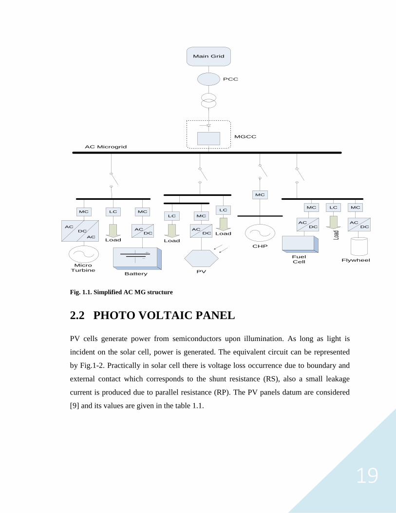
2.1 SYSTEM DESCRIPTION

For the project, an AC micro-grid is assumed to consist of group of distributed loads and

distributed energy low voltage sources, such as PV panels, Wind turbine generators

(WTGs), Diesel engine generators (DEGs), Fuel cells (FCs) and energy storage devices

such as Flywheel energy storage system (FESS) and Battery energy storage system

(BESS). The simplified MG architecture is shown in fig 1-1.

AC sources like DEG and WED are synchronized and DC sources like PV panels, FCs

and Energy storage systems are integrated to the AC Micro grid structure using Power

electronic interfaces. Each DG has its own individual circuit breaker, which disconnects

it from system during lethal grid disturbances to protect it from the fault impact.

The MG model is an isolated Hybrid Renewable power generation model. Detailed in

corresponding clauses are shown in the figure 1.1 where the local loads and controllers

are connected [4].

19

Main Grid

MC LC MC

MC

LC MC

MC LC MC

DC

ACDC

ACAC

ACDC

AC

DC

AC

DC

Flywheel

Load

Fuel

Cell

CHP

PVBattery

Micro

Turbine

Load Load

LC

Load

AC Microgrid

PCC

MGCC

Fig. 1.1. Simplified AC MG structure

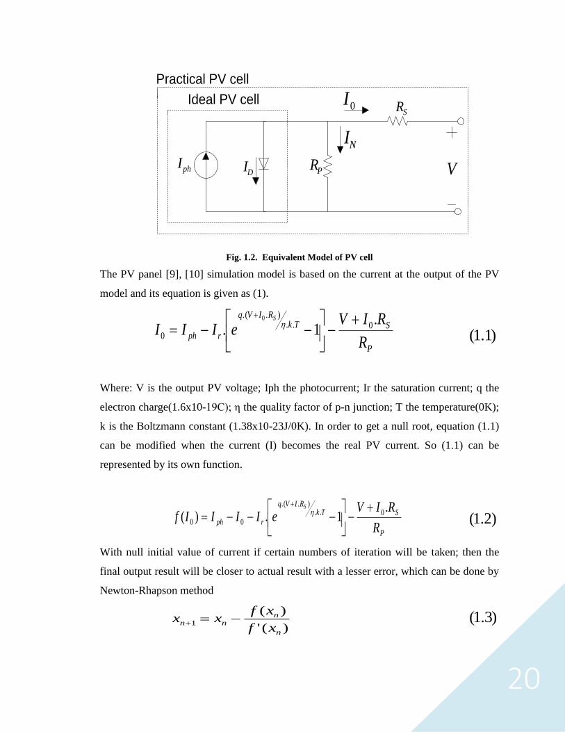
2.2 PHOTO VOLTAIC PANEL

PV cells generate power from semiconductors upon illumination. As long as light is

incident on the solar cell, power is generated. The equivalent circuit can be represented

by Fig.1-2. Practically in solar cell there is voltage loss occurrence due to boundary and

external contact which corresponds to the shunt resistance (RS), also a small leakage

current is produced due to parallel resistance (RP). The PV panels datum are considered

[9] and its values are given in the table 1.1.

20

phIDI PR

SR

V

Ideal PV cell

Practical PV cell

NI

0I

Fig. 1.2. Equivalent Model of PV cell

The PV panel [9], [10] simulation model is based on the current at the output of the PV

model and its equation is given as (1).

P

STkRIVq

rphR

RIVeIII

S .1. 0..

)..(

0

0

)1.1(

Where: V is the output PV voltage; Iph the photocurrent; Ir the saturation current; q the

electron charge(1.6x10-19C); η the quality factor of p-n junction; T the temperature(0K);

k is the Boltzmann constant (1.38x10-23J/0K). In order to get a null root, equation (1.1)

can be modified when the current (I) becomes the real PV current. So (1.1) can be

represented by its own function.

P

STkRIVq

rphR

RIVeIIIIf

S .1.)( 0..

)..(

00

)2.1(

With null initial value of current if certain numbers of iteration will be taken; then the

final output result will be closer to actual result with a lesser error, which can be done by

Newton-Rhapson method

)('

)(1

n

nnn

xf

xfxx )3.1(

21

Thus the derivative of (1.3) will be (1.4)

P

SSTkRIVq

rR

R

Tk

RqeIIf S

..

.1)(

..)..( 0

)4.1(

Electrical parameters of the PV [9]

TABLE- 1-1 PV MODEL DATA

Maximum Power Pmax = 30kW

Voltage at MPP VMPP = 34.5V

Current at MPP IMPP = 4.35A

Open Circuit Voltage Voc = 43.5V

Short Circuit Current Isc = 4.75A

Temperature Coefficient of Isc 0.065 A/oC

NO of series Cell 06

NO of parallel Cell 10

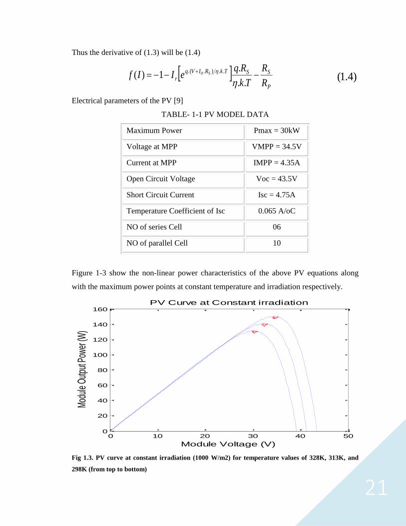
Figure 1-3 show the non-linear power characteristics of the above PV equations along

with the maximum power points at constant temperature and irradiation respectively.

Fig 1.3. PV curve at constant irradiation (1000 W/m2) for temperature values of 328K, 313K, and

298K (from top to bottom)

0 10 20 30 40 500

20

40

60

80

100

120

140

160PV Curve at Constant irradiation

Module Voltage (V)

Mod

ule

Outp

ut P

ower

(W)

22

Fig. 1.4. Right side curves are at constant temperature of 298K and irradiance values of 200,400,600,800

and 1000W/m2 (from top to bottom).

2.3 WIND TURBINE GENERATOR

In the present system's Wind Energy extraction System, wind turbine is modeled as in

[11-12]. The generated power in the WTG is related to the wind velocity(VW). The rotor

mechanical power(PW) produced by the wind turbine is given by equation (1.5)

Pw =1

2ρArCp(γ, β)Vw

3 (1.5)

This equation is used to model the performance coefficient of the wind turbine as a

function of tip speed ratio and blade pitch angle as given in Equation (1.5). It is based on

turbine characteristics in [11]. The tip speed ratio is defined as the ratio of the speed at

the tip of the blade to the wind velocity.

Cp(γ, β) = C1 (C2

γi

− Caβ − C4) e−C5

γi − C6γ (1.6)

0 10 20 30 40 500

20

40

60

80

100

120

140

160PV Curve at Constant temperature

Module Voltage (V)

Mod

ule

Out

put P

ower

(W)

23

Equation for γi is given as equation (1.7). The coefficient C1 to C6 are:- C1 =0.5176, C2

=116, C3=0.4, C4=5, C5=21 and C6=0.0068

1

γi=

1

γ+0.08β−

0.035

β3+1 (1.7)

The wind turbine model considered in the study is with WT having prototype as given in

[11]. For a typical wind turbine blade radius here is taken as 18m, and the rotational

speed of the blade is taken as 3.14rad/s. The air density ρ is 1.25kg/m3 and swept area of

blades is considered as Ar is 1018 m^2. By taking the above parameters into

consideration, the following Table 1-1 is constructed which shows the mechanical output

at different speed with different tip ratio and its' corresponding power coefficient.

The wind model which is considered here for the purpose of the study is providing a rated

output of 190kW. But actual rated output of WT is 216W at 10m/s, which simply states

that it has a conversion efficiency of 88.3% approximately for the associated gear system

plus generator. The cut-in wind velocity for the WT is 4.22m/s. A cut-out velocity of

18m/s is considered for the machine. For wind velocity of 10m/s up to 18m/s, blade pitch

control can be done to achieve rated output of 216kW from the turbine. Wind turbine

speed from 4m/sec to 10m/sec the power varies approximately linearly with the speed of

the wind and after that due to stall control the power is going to be constant irrespective

of the wind turbine speed and due to this the turbine is safe from the high wind speed.

Now after that if the wind speed is going beyond the speed of 18m/sec at that time the

controller will force the turbine speed to come to zero and that moment the turbine will

deliver no power and power cannot be extracted at that time. Here the important thing to

be noted that due to the use of stall controller up to some level the power is going to be

constant, irrespective of wind speed and beyond that speed the power delivered to the

system will be zero but the turbine at that time will be rotated more than the rated speed.

And this is done in order to save the turbine from damage from this type of high speed.

The blade pitch control is achieved in the Simulink model through ‘look-up block’

characteristics curve i.e. output mechanical power versus wind speed for the study of

WT, as shown in Fig 1-4.

24

TABLE 1-2

Wind Velocity

(Vw)in m/sec

Tip Speed ratio (γ) Blade Pitch

angle(β) in

degree

Coefficient Mechanical

Power output

in watts(Pw)

4

4.22

4.6

5

6

7

7.191

8

9

9.5

10

11

11.5

12

12.5

13

13.5

14

14.5

15

15.5

16

16.5

17

17.5

18

19

0

13.4

12.29

11.31

9.42

8.08

7.86

7.07

6.28

5.95

5.65

5.14

4.92

4.71

4.52

4.35

4.19

4.04

3.9

3.77

3.65

3.53

3.43

3.33

3.23

3.14

2.98

0

0

0

0

0

0

0

0

0

0

0

0.7

0.796

0.864

0.911

0.939

0.951

0.948

0.933

0.906

0.87

0.825

0.773

0.712

0.64

0.55

0

0

0.0003

0.1572

0.2786

0.4418

0.48

0.4787

0.4548

0.4016

0.371

0.34

0.2554

0.2235

0.1967

0.1741

0.1547

0.1382

0.1239

0.1115

0.1007

0.091

0.083

0.0757

0.0692

0.0634

0.0583

0.0481

0

13

9731

22157

60706

104740

113244

148130

186233

202367

216287

216287

216287

216287

216287

216287

216287

216287

216287

216287

216287

216287

216287

216287

216287

216287

209819

25

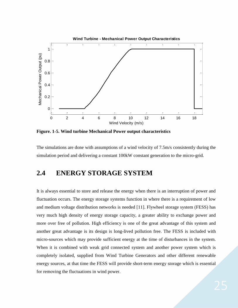
Figure. 1-5. Wind turbine Mechanical Power output characteristics

The simulations are done with assumptions of a wind velocity of 7.5m/s consistently during the

simulation period and delivering a constant 100kW constant generation to the micro-grid.

2.4 ENERGY STORAGE SYSTEM

It is always essential to store and release the energy when there is an interruption of power and

fluctuation occurs. The energy storage systems function in where there is a requirement of low

and medium voltage distribution networks is needed [11]. Flywheel storage system (FESS) has

very much high density of energy storage capacity, a greater ability to exchange power and

more over free of pollution. High efficiency is one of the great advantage of this system and

another great advantage is its design is long-lived pollution free. The FESS is included with

micro-sources which may provide sufficient energy at the time of disturbances in the system.

When it is combined with weak grid connected system and another power system which is

completely isolated, supplied from Wind Turbine Generators and other different renewable

energy sources, at that time the FESS will provide short-term energy storage which is essential

for removing the fluctuations in wind power.

0 2 4 6 8 10 12 14 16 18

0

0.2

0.4

0.6

0.8

1

Wind Velocity (m/s)

Mechanic

al P

ow

er

Outp

ut

(pu)

Wind Turbine - Mechanical Power Output Characteristics

26

Battery energy storage system (BESS) [11] is also one typo which stores electric energy inform

of DC as like in the battery and when it connects to the ac grid it needs a rectifier circuit, and a

dc–ac inverter so that there is an exchange of energy will be there in between the AC system.

In the last decade, the advancement in sealing procedure, recombinant of the lead-acid battery

technology, and also the finest advancement in the compounds have increased the scope utility

in term of economic and regarding the applications of the BESS. The used transfer function and

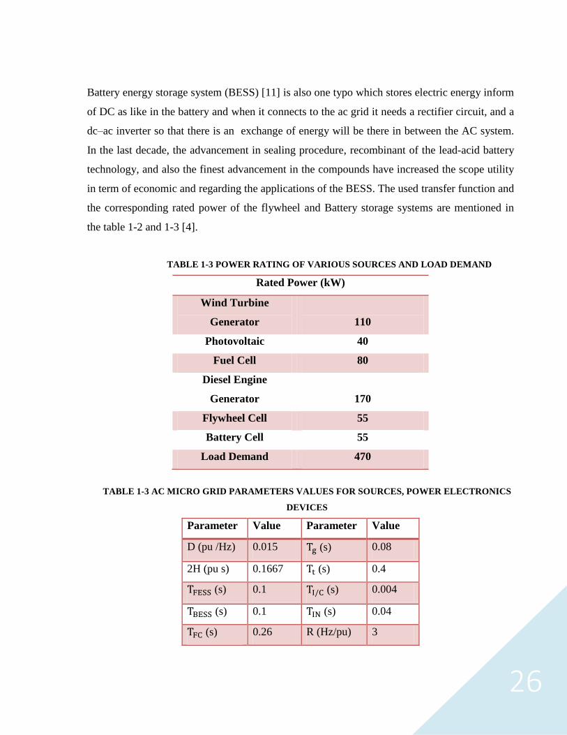
the corresponding rated power of the flywheel and Battery storage systems are mentioned in

the table 1-2 and 1-3 [4].

TABLE 1-3 POWER RATING OF VARIOUS SOURCES AND LOAD DEMAND

Rated Power (kW)

Wind Turbine

Generator

110

Photovoltaic 40

Fuel Cell 80

Diesel Engine

Generator

170

Flywheel Cell 55

Battery Cell 55

Load Demand 470

TABLE 1-3 AC MICRO GRID PARAMETERS VALUES FOR SOURCES, POWER ELECTRONICS

DEVICES

Parameter Value Parameter Value

D (pu /Hz) 0.015 Tg (s) 0.08

2H (pu s) 0.1667 Tt (s) 0.4

TFESS (s) 0.1 TI/C (s) 0.004

TBESS (s) 0.1 TIN (s) 0.04

TFC (s) 0.26 R (Hz/pu) 3

27

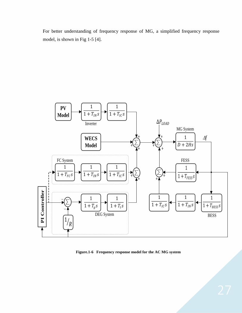
For better understanding of frequency response of MG, a simplified frequency response

model, is shown in Fig 1-5 [4].

DfWECS

Model

PI C

on

tro

ller

∆𝑃𝐿𝑂𝐴𝐷

1

1 + 𝑇𝑔𝑠

1

1 + 𝑇𝑡𝑠

1𝑅

DEG System

1

1 + 𝑇𝐼𝑁𝑠

1

1 + 𝑇𝐼𝐶𝑠

1

1 + 𝑇𝐹𝐶𝑠

FC System

1

1 + 𝑇𝐼𝑁𝑠

1

1 + 𝑇𝐼𝐶𝑠 PV

Model

Inverter

1

𝐷 + 2𝐻𝑠

MG System

1

1 + 𝑇𝐹𝐸𝑆𝑆𝑠

FESS

1

1 + 𝑇𝐵𝐸𝑆𝑆𝑠

1

1 + 𝑇𝐼𝑁𝑠

1

1 + 𝑇𝐼𝐶𝑠

BESS

Figure.1-6 Frequency response model for the AC MG system

28

FREQUENCY CONTROL AND

SECONDARY CONTROLLER TUNING

AND FUZZY IMPLEMENTATION

Secondary frequency regulation

Ziegler-Nicholas method

Fuzzy logic implementation

Static load modelling

Dynamic load modelling

29

3.1 SECONDARY FREQUENCY REGULATION

In the present system natural frequency regulation is provided by rotational inertia and the only

rotational inertia source available is the DEG. DEG is provided with a PI based secondary

controller. The same signal from this controller is used for FC system also. But it is not the

same PI controller used in FC, because the droop used for DG will generate a separate error

signal for the DG set which is not the same as that for the FC signal [4].

For the MG system, secondary controller is to be tuned for proportional gain (Kp) and integral

gain (Ki) such that the frequency is restored to the specified nominal value under load or

generation variation. In traditional power systems, tuning is done with a very small step load

perturbation with respect to a pre-specified operating point. If the PI controller continuously

keeps track of the changes occurring in the power system and change the Kp and Ki values

accordingly in real time, optimal performance will be achieved. Fluctuation in load and

generation are of compatible amount in terms of MG system capacity. Hence, response studies

are done with a practical generation-load imbalance possible in the system, which is considered

of the order of 20-40%. Frequency control action on the MG system is done by secondary

controllers, which are tuned by the following two methods.

3.2 ZIEGLER-NICHOLAS METHOD

Ziegler–Nicholas is one of upmost method to design the tuning parameter of the PI

controller, where at first the Ki (integral) and Kd (derivative) gains are required to set at zero

value. Then the Kp (proportional) gain, has be increased (from zero) until it reaches to

sustain oscillation and at that time the value of the gain will be the ultimate gainKu, Ku when

this oscillation will reach the time period will be Tu which is used to get the Ki, Kd and Kp

values depending on which type of the controller we are using in the system [16].

TABLE1.4 ZEIGLER NICHOLAS CONTROLLER VALUES

Control Type Kp Ki Kd

P Ku/2 -

PI Ku/2.2 1.2Kp/Tu -

PID 0.60Ku 2Kp/Tu TuKp/8

30

3.3 FUZZY LOGIC IMPLEMENTATION In order to have better performance, a better way for online tuning of the PI controller is by

using fuzzy logic, as shown in fig 1-7. A fuzzy PI controller consist of two stages. Stage one

is fuzzy system unit where frequency deviation (∆f) and the change of load power to the

source power (∆P) are taken as input variables and after that fuzzy rules are incorporated

and as far as the mentioned rules, the output variables (proportional gain,𝐾𝑝 and integral

gain,𝐾i) are calculated by the fuzzy set and supplied to the PI controller for tuning. An

important thing needed to be considered here is that at the time of large number of loads, it

is always difficult to calculate the difference of the power and frequency being fed to the

fuzzy logic controller [8]. Hence, secondary frequency control is important and is calibrated

by tuning the PI controller but in changeable operating condition it doesnot give an optimal

solution.

PI Controller Plant

Fuzzy System

pK

iK

fDrefF

fD

loadPD

Figure.1-7. Secondary frequency control with fuzzy PI

31

TABLE 1-5 THE FUZZY RULES SET

∆𝐏/∆𝐟 NL NM NS PS PM PL

S NL NM NS PS PS PM

M NL NL NM PS PM PM

L NL NL NL PM PM PM

The membership functions of the input and output variables are categorised as Positive

Small (PS),Positive Medium (PM), Positive Large (PL), Negative Large (NL), Negative

Medium (NM) and Negative Small (NS),. The fuzzy logic codes are written in the fis.file in

MATLAB where all 18 rules are written. Then AND function is used with Mamdani

environment by using the Triangular Membership function. [4], [8]. Here in fuzzy based PI

controller tuning operation, all the rules are mentioned based on the system consideration

and while performing this, it is very much depends on the membership function which are

being chosen by us, because of this thing all the rules has to select with a great consideration

and should be bounded according to the input and output values. So in order to avoid this

type of hindrance it is always advisable to choose other optimized algorithm with fuzzy

logic so the more dependence thing will be eliminated.

3.4 STATIC LOAD MODELLING

For the modelling of the static load, it can be considered as the step input and according to

the step input it is given as the load variable and the system simulation is being performed.

At first the system is run through the conventional PI controller which is being tuned by the

Zeigler-Nicholas method and after that it was being tuned by the fuzzy logic based tuning

method and the corresponding results are being obtained. For more analysis, the various

changing of the load are taken in to consideration and corresponding frequency deviation are

shown in the Fig 1.21.

3.5 DYNAMIC LOAD MODELLING

For exact validation of the frequency deviation, an induction motor having a 5th order

transfer function is considered as dynamic load. In order to build the transfer function model

of the induction motor [13], state space average method is taken into account and the

32

parameters are being referred as far as the reference [13], [8]. While designing the induction

motor model it is very much important to consider its inertia. It has always one inertia and

our system has also some short of inertia and when both the inertia are being combined at

that time the system will be much more rigid and stable as compare to old static system.

Now this model of induction motor is one type of real time example and all our practical

loads are having some short of inertia.

The second important thing need to be considered that all the system has its own time

constant and it is applicable to all the system but in the static load there is no time constant.

Due to this time constant the system will always exhibit some short of time delay, other time

delays are coming due to inclusion of wind turbine, diesel turbine, battery or flywheel. So

whenever the induction motor torque changes the output power also changes accordingly

and that change of power cause the change in the load demand. So here the step in the load

torque is being performed and its corresponding output change is considered as load change

and then it is applied to the system and its result are shown in the corresponding figure. Here

the insertion of DG, the inertia constant (H) is coming and both are loaded it is always

considered as one stable system.

Damping coefficient (D) is also one of important factor in consideration to the system. The

presence of the induction motor load and the other damping coefficient which is coming due

to turbine rotor mass which are accumulated and finally giving an effective damping factor

which is higher than the previous one. Due to this increase in the damping and inertia

parameter the overall system will be very rigid and stable. And due to this the frequency

deviation is this type of dynamic load is quite less as compare to the static one [13], [8].

Here, for static and dynamic load, various step changes in loads are considered and its

corresponding frequency deviation are depicted in Fig.1.8, 1.9 respectively. From the above

result it is always being found that the fuzzy logic tuned PI controller is providing better

performance as compare to the other one.

33

Fig 1.8: Fuzzy Logic Set

Fig 1.9 Fuzzy Logic input membership function (del(f))

34

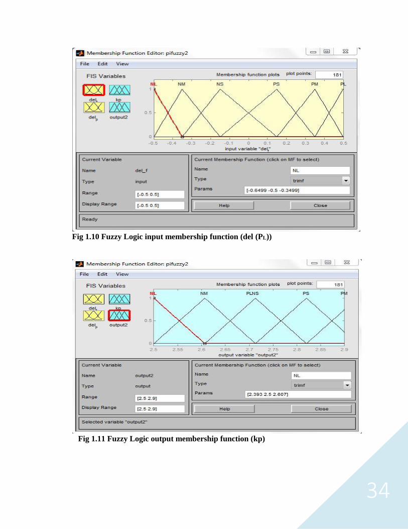
Fig 1.10 Fuzzy Logic input membership function (del (PL))

Fig 1.11 Fuzzy Logic output membership function (kp)

35

Fig1.12 Fuzzy Logic output membership function (ki)

Fig1.13 Fuzzy Logic input/output membership function with graphical rules

36

Fig1.14 Fuzzy Logic input/output membership function with rules

Fig1.15 Fuzzy Logic three dimensional surface function representation

37

RESULTS AND DISCUSSION

Simulation results of LFC

Analysis and result

Discussion

38

4.1 SIMULATION RESULT OF LFC

FIG 1.16: Comparison between frequency tuning in PI controller and Fuzzy PI

controller of Static load

FIG 1.17: Step Response of Dynamic Load

FIG 1.18: Comparison between frequency tuning in PI controller and Fuzzy PI

controller of Dynamic Load

6 7 8 9 10 11 12 13 14-0.08

-0.06

-0.04

-0.02

0

0.02

0.04

Time(sec)

del(f

)

Fuzzy PI Controller

PI Controller

6 8 10 12 14 16 18 20 220

0.01

0.02

0.03

0.04

0.05

0.06

0.07

Time(sec)

del(p

L)

6 8 10 12 14 16 18 20 22-6

-5

-4

-3

-2

-1

0

1

2

3x 10

-3

Time(sec)

de

l(f)

Fuzzy PI COntroller

PI Controller

39

FIG 1.19: Comparison between frequency tuning in PI controller and Fuzzy PI

controller of Dynamic Load for 0.1pu of change of load power

Fig1.20 Frequency tuning comparison under varying parameters

TABLE 1-7 UNCERTAIN PARAMETERS AND VARIATION RANGE Parameter Variation

Range

Parameter Variation

Range

R +30% Tg +50%

D -40% TFESS -45%

H +50% TBESS +55%

Tt -50%

6 7 8 9 10 11 12 13 14-0.03

-0.02

-0.01

0

0.01

Time(sec)

del(f)

Fuzzy PI Controller

PI Controller

6 8 10 12 14 16 18-0.06

-0.05

-0.04

-0.03

-0.02

-0.01

0

0.01

0.02

0.03

Time(sec)

de

l(f)

Fuzzy PI Controller

PI Controller

40

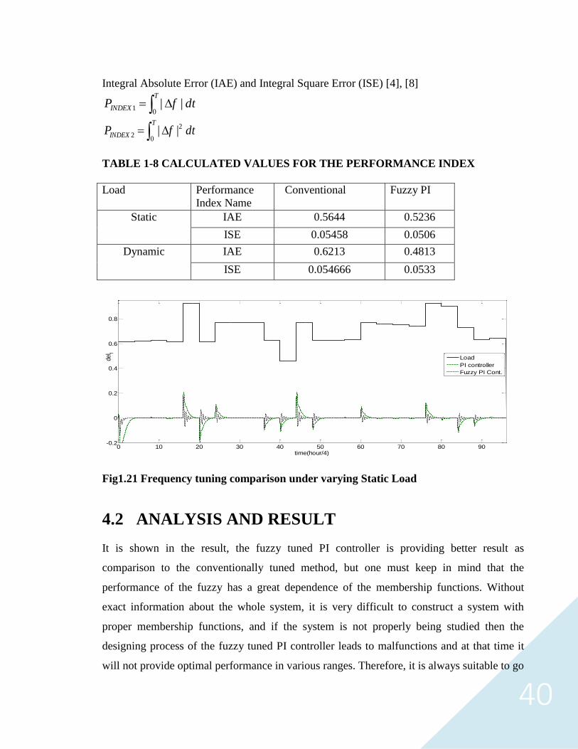
Integral Absolute Error (IAE) and Integral Square Error (ISE) [4], [8]

DT

INDEX dtfP0

1 ||

DT

INDEX dtfP0

2

2 ||

TABLE 1-8 CALCULATED VALUES FOR THE PERFORMANCE INDEX

Load Performance

Index Name

Conventional Fuzzy PI

Static IAE 0.5644 0.5236

ISE 0.05458 0.0506

Dynamic IAE 0.6213 0.4813

ISE 0.054666 0.0533

Fig1.21 Frequency tuning comparison under varying Static Load

4.2 ANALYSIS AND RESULT

It is shown in the result, the fuzzy tuned PI controller is providing better result as

comparison to the conventionally tuned method, but one must keep in mind that the

performance of the fuzzy has a great dependence of the membership functions. Without

exact information about the whole system, it is very difficult to construct a system with

proper membership functions, and if the system is not properly being studied then the

designing process of the fuzzy tuned PI controller leads to malfunctions and at that time it

will not provide optimal performance in various ranges. Therefore, it is always suitable to go

0 10 20 30 40 50 60 70 80 90-0.2

0

0.2

0.4

0.6

0.8

time(hour/4)

del f

Load

PI controller

Fuzzy PI Cont.

41

for complementary algorithm which can be used to regulate the controller by online method

with the use of membership functions. From the above figure data represented in the Fig

1.21, it is seen that, at every hour, the load is different and due to this changing of load, the

deviation in the frequency is happening and for that the oscillation in the frequency occurs.

4.3 DISCUSSION

In the above figures, the comparison between the PI controller of conventional type and

fuzzy PI controller is being performed and from the figures also it is clearly being stated that

the fuzzy logic is providing a better result as compare to conventional one. In order to make

the result more prominent the errors are taken and there also it is seen that the fuzzy logic

stabilizes more in a faster way as compared to the conventional one and that’s why the error

is very less in fuzzy. Here the use 5th order induction motor load provides a define time

delay which is not being performed by the static load and this load has some short of inertia

(parameters mentioned in the appendix) and due to this inertia and the system inertia making

the system more and more stable and due to this the frequency is going to be stabilized in a

faster way as compared to the static load and for this dynamic load the error is also less

compared to the static one.

42

CONCLUSION AND FUTURE WORK

Conclusion

Future Work

43

5.1 CONCLUSION

In this thesis, micro grids and their control have been reviewed. Frequency regulation is

an essential component of ac micro-grids during the presence of disturbances and load

changes. Usually, the output of a conventional PI controller varies significantly with the

changes in surrounding and in presence of disturbance.

In conventional power systems, there is greater need of secondary frequency control

requires and it is usually being done by using conventional PI controllers and at that time the

flywheel storage system and diesel engine system need a greater role in order to stabiles the

frequency. If there is a requirement of any change in the operating conditions, at that time it

is difficult for the PI controllers to provide the desired performance. But, if we make the

system in such a way that the PI controllers can keep a continuous track of the system

changes in the power system, then the optimal performance will be always achieved in a

better way. Any who Fuzzy logic can also be useful for suitable and intelligent control for

online tuning of the PI controller parameters.

5.2 FUTURE WORK

Here in this model the fuzzy PI controller is implemented and now a days many

others methods are being developed. Various evolutionary algorithm like particle

swarm optimization, bacteria foraging, radial basis function, and neural logic

network have to be implemented.

Here only frequency controller is being designed but in the real time when there

is a power interruption both the voltage and frequency dip occur, so the use of

reactive power in order to stabilize the system has to be done.

The system model has to be in such a way that both voltage and frequency control

be done at a time with a different controller not separately.

44

REFERENCES

1) S Prakash,. S.K. Sinha, “Intelligent PI control technique in four area Load

Frequency Control of interconnected hydro-thermal power system”Computing,

Electronics and Electrical Technologies (ICCEET), 2012 International

Conference on Digital Object Identifier ,vol. 12,no.5, pp: 145 – 150, Oct. 2012.

2) R. H. Lasseter, A. Akhil, C. Marnay, J. Stephens, J. Dagle, R. Guttromson, A.

Meliopoulous, and R. J. Yinger, “The CERTS microgrid concept,” White Paper,

Transmission Reliability Program, Office of Power Technologies, U.S. Dept.

Energy,, Apr. 2.

3) Y. H. Li, S. S. Choi, and S. Rajakaruna, “An analysis of the control and operation

of a solid oxide fuel-cell power plant in an isolated system,” IEEE Trans. Energy

Convers., vol. 20, no. 2, pp. 381–387, Jun. 2005.

4) Bevrani, H; Habibi, F; Babahajyani, P; Watanabe, M; Mitani, Y., "Intelligent

Frequency control in an AC Microgrid: Online PSO-Based Fuzzy Tuning

Approach," Smart Grid, IEEE Transactions on , vol.3, no.4, pp.1935,1944, Dec.

2012

5) Rabbani, M.; Maruf, H.M.M.; Ahmed, T.; Kabir, M.A.; Mahbub, U., "Fuzzy logic

driven adaptive PID controller for PWM based buck converter," Informatics,

Electronics & Vision (ICIEV), 2012 International Conference on , vol., no.,

pp.958,962, 18-19 May 2012

6) Daneshfar, F.; Bevrani, H., "Load-frequency control: a GA-based multi-agent

reinforcement learning," Generation, Transmission & Distribution, IET , vol.4,

no.1, pp.13,26, January 2010

7) Bevrani, H.; Daneshmand, P.R.; Babahajyani, P.; Mitani, Y.; Hiyama, T.,

"Intelligent LFC Concerning High Penetration of Wind Power: Synthesis and

Real-Time Application,"Sustainable Energy, IEEE Transactions on , vol.5, no.2,

pp.655,662, April 2014

8) Dash, K Mahesh; Sahoo, Subham; Mishra, Sukumar, "A detailed analysis of

optimized load frequency controller for static and dynamic load variation in an

AC microgrid," Condition Assessment Techniques in Electrical Systems

(CATCON), 2013 IEEE 1st International Conference on , vol., no., pp.17,22, 6-8

Dec. 2013

9) Satapathy, S.; Dash, K.M.; Babu, B.C., "Variable step size MPPT algorithm for

photo voltaic array using zeta converter - A comparative analysis," Engineering

and Systems (SCES), 2013 Students Conference on , vol., no., pp.1,6, 12-14 April

2013

45

10) H. Patel and V. Agarwal, “MATLAB-based modeling to study the effects of partial

shading on PV array characteristics”, IEEE Trans. Energy Convers., vol. 23, no.

1, pp. 302–310, Mar. 2008

11) D.J. Lee and L. Wang, “Small-signal stability analysis of an autonomous hybrid

renewable energy power generation/energy storage system part I: Time-domain

simulations,” IEEE Trans. Energy Convers., vol. 23, no. 1, pp. 311–320, 2008.

12) P. M. Anderson and A. Bose, “Stability simulation of wind turbine system,” IEEE

Trans. Power App. Syst., vol. 102, no. 12, pp. 3791–3795, Dec. 2010

13) Alexandrovitz, A.; Lechtman, S., "Dynamic behaviour of induction motor based

on transfer-function approach," Electrical and Electronics Engineers in Israel,

1991. Proceedings, 17th Convention of, vol., no., pp.328,333, 5-7 Mar 1991.

14) Daugherty, R.H., "Analysis of Transient Electrical Torques and Shaft Torques in

Induction Motors as a Result of Power Supply Disturbances," Power Engineering

Review, IEEE, vol.PER-2, no.8, pp.55,55, Aug. 1982.

15) Yousef, H.A.; AL-Kharusi, K.; Albadi, M.H.; Hosseinzadeh, N., "Load

Frequency Control of a Multi-Area Power System: An Adaptive Fuzzy Logic

Approach," Power Systems, IEEE Transactions on , vol.PP, no.99, pp.1,9.

16) Kumar, A.; Kumar, A.; Chanana, S., "Genetic fuzzy PID controller based on

adaptive gain scheduling for load frequency control," Power Electronics, Drives

and Energy Systems (PEDES) & 2010 Power India, 2010 Joint International

Conference on , vol., no., pp.1,8, 20-23 Dec. 2010

CODES FUZZY LOGIC CODE

[System] Name='pifuzzy2' Type='mamdani' Version=2.0 NumInputs=2 NumOutputs=2 NumRules=18 AndMethod='min' OrMethod='max' ImpMethod='min' AggMethod='max' DefuzzMethod='centroid' range=2;

[Input1] Name='del_f' Range=[-0.7 0.5] NumMFs=6 MF1='NL':'trimf',[-0.94 -0.7 -0.46] MF2='NM':'trimf',[-0.7 -0.46 -0.22]

46

MF3='NS':'trimf',[-0.46 -0.22 0.02] MF4='PS':'trimf',[-0.22 0.02 0.26] MF5='PM':'trimf',[0.02 0.26 0.5] MF6='PL':'trimf',[0.26 0.5 0.74] [Input2] Name='del_p'

Range=[0 0.2] NumMFs=3 MF1='S':'trimf',[-0.08 0 0.08] MF2='M':'trimf',[0.02 0.1 0.18] MF3='L':'trimf',[0.12 0.2 0.28]

[Output1] Name='kp' Range=[0 2] NumMFs=6 MF1='NL':'trimf',[-0.4 0 0.4] MF2='NM':'trimf',[0 0.4 0.8] MF3='NS':'trimf',[0.4 0.8 1.2] MF4='PS':'trimf',[0.8 1.2 1.6] MF5='PM':'trimf',[1.2 1.6 2] MF6='PL':'trimf',[1.8 1.9973544973545 2.25]

[Output2] Name='output2' Range=[0 2] NumMFs=6 MF1='NL':'trimf',[-0.4 6.94e-018 0.4] MF2='NM':'trimf',[0 0.4 0.8] MF3='NS':'trimf',[0.4 0.8 1.2] MF4='PS':'trimf',[0.8 1.2 1.6] MF5='PM':'trimf',[1.2 1.6 2] MF6='PL':'trimf',[1.6 2 2.]

[Rules] 1 1, 1 1 (1) : 1 2 1, 2 2 (1) : 1 3 1, 3 3 (1) : 1 4 1, 4 4 (1) : 1 5 1, 4 4 (1) : 1 6 1, 5 5 (1) : 1 1 2, 1 1 (1) : 1 2 2, 1 1 (1) : 1 3 2, 2 2 (1) : 1 4 2, 4 4 (1) : 1 5 2, 5 5 (1) : 1 6 2, 6 6 (1) : 1 1 3, 1 1 (1) : 1 2 3, 1 1 (1) : 1 3 3, 1 1 (1) : 1 4 3, 5 5 (1) : 1 5 3, 5 5 (1) : 1 6 3, 5 5 (1) : 1

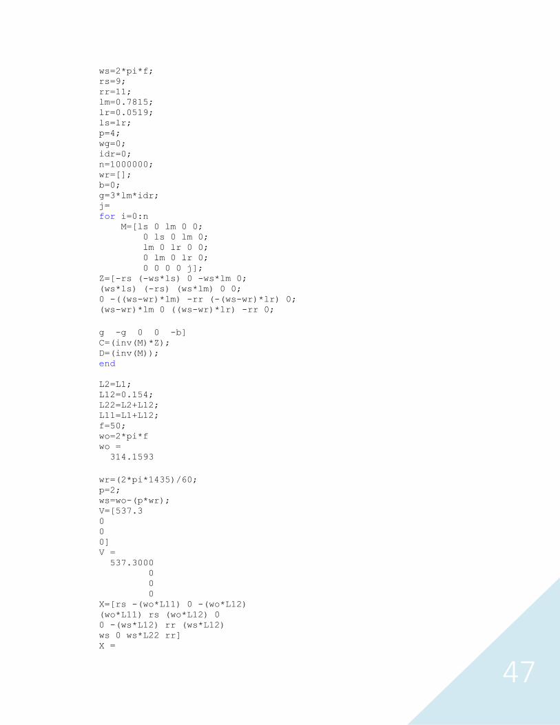
INDUCTION MOTOR CODE f=50;

47

ws=2*pi*f; rs=9; rr=11; lm=0.7815; lr=0.0519; ls=lr; p=4; wg=0; idr=0; n=1000000; wr=[]; b=0; g=3*lm*idr; j= for i=0:n M=[ls 0 lm 0 0; 0 ls 0 lm 0; lm 0 lr 0 0; 0 lm 0 lr 0; 0 0 0 0 j]; Z=[-rs (-ws*ls) 0 -ws*lm 0; (ws*ls) (-rs) (ws*lm) 0 0;

0 -((ws-wr)*lm) -rr (-(ws-wr)*lr) 0; (ws-wr)*lm 0 ((ws-wr)*lr) -rr 0;

g -g 0 0 -b] C=(inv(M)*Z); D=(inv(M)); end

L2=L1; L12=0.154; L22=L2+L12; L11=L1+L12; f=50; wo=2*pi*f wo = 314.1593

wr=(2*pi*1435)/60; p=2; ws=wo-(p*wr); V=[537.3 0 0 0] V = 537.3000 0 0 0 X=[rs -(wo*L11) 0 -(wo*L12) (wo*L11) rs (wo*L12) 0 0 -(ws*L12) rr (ws*L12) ws 0 ws*L22 rr] X =

48

1.3150 -72.8221 0 -48.3805 72.8221 1.3150 48.3805 0 0 -2.0965 1.1920 2.0965 13.6136 0 3.1556 1.1920 Y=inv(X) Y = 0.0010 -0.0059 -0.0374 0.1051 -0.0085 0.0066 -0.1769 -0.0346 -0.0012 0.0294 0.0611 -0.1573 -0.0078 -0.0101 0.2653 0.0549 I=Y*V I = 0.5208 -4.5771 -0.6595 -4.2021 I'=V*Y det=(L11*L22)-(L12)^2 a11=-(rs*L22)/det; a22=a11; a12=(wo*L11*L22)-(ws*(L12)^2); a21=-a12; a13=(rr*L12)/det; a24=a13; a14=(wo*L12*L22-ws*L12*L22)/det; a12=((wo*L11*L22)-(ws*(L12)^2))/det; a21=-a12; a15=((p*L12*6.5208+L22*(-4.2021))*L12)/det; a15=p*((L12*6.5208+L22*(-4.2021))*L12)/det; a25=-p*((L12*6.5208+L22*(-4.2021))*L12)/det; a15=p*((L12*(-4.5771)+L22*(-4.2021))*L12)/det; a25=-p*((L12*(6.5208)+L22*(-0.6595))*L12)/det; a31=(rs*L12)/det; a42=a31; a32=(wo*L12*L11-ws*L12*L11)/det; a41=-(a32); a33=(-rr*L11)/det; a44=a33; a34=-(wo*(L12^2)-ws*L11*L22)/det; a43=-a34; a35=-(p*(L12*(-4.5771)+L22*(-4.2021))*L11)/det; a45=(p*(L12*(6.5208)+L22*(-0.6595))*L11)/det; j=0.047; a51=(-3*L12*(-4.2021))/j; a52=3*L12*(-0.6595)/j; a53=3*L12*(-4.5771)/j; a55=0; a54=-3*L12*6.5208/j; b11=L22/det; b22=b11; b33=L11/det; b44=b33; b13=(-L12)/det; b24=b13; b31=b13; b42=b13; s=0.043;

49

N1=-(L11*(4.5771)+L12*(-4.2021)); N2=(L11*(6.5208)+L12*(-0.6595)); N3=-s*(L12*(-4.5771)+L22*(-4.2021)); N4=s*(L12*(6.5208)+L22*(-0.6595)); b16=(N3*L12-N1*L22)/det; b26=(N4*L12-N2*L22)/det; b36=(N1*L12-N3*L11)/det; b46=(N2*L12-N4*L11)/det; b12=b14=b15=b21=b23=b25=b32=b34=b35=b41=b43=b45=b51=b52=b53=b54=b56=0; ???

b12=b14=b15=b21=b23=b25=b32=b34=b35=b41=b43=b45=b51=b52=b53=b54=b56=0; b12=b14=b15=0; b12=b14=0 B=[b11 0 b13 0 0 b16 0 b22 0 b24 0 b26 b31 0 b33 0 0 b36 0 b42 0 b44 0 b46 0 0 0 0 b55 0] b55=-(1/(j*det)); B=[b11 0 b13 0 0 b16 0 b22 0 b24 0 b26 b31 0 b33 0 0 b36 0 b42 0 b44 0 b46 0 0 0 0 b55 0] B =

7.7227 0 -5.1307 0 0 3.5665 0 7.7227 0 -5.1307 0 -10.7009 -5.1307 0 7.7227 0 0 -2.6809 0 -5.1307 0 7.7227 0 6.9514 0 0 0 0 -708.8598 0 A=[a11 a12 a13 a14 a15 a21 a22 a23 a24 a25 a31 a32 a33 a34 a35 a41 a42 a43 a44 a45 a51 a52 a53 a54 a55] a23=0; A=[a11 a12 a13 a14 a15 a21 a22 a23 a24 a25 a31 a32 a33 a34 a35 a41 a42 a43 a44 a45 a51 a52 a53 a54 a55]

A = -10.1554 551.6300 6.1158 357.4397 -17.2282 -551.6300 -10.1554 0 6.1158 -8.7359 6.7469 357.4397 -9.2055 -223.8572 25.9317 -357.4397 6.7469 223.8572 -9.2055 13.1492 41.3057 -6.4827 -44.9919 -64.0981 0 L=-(3/2)*p*L12; C=[L*(-4.2021) L*0.6595 L*4.5771 L*6.5208 0]

C = 1.9414 -0.3047 -2.1146 -3.0126 0

D=[0];

50

sys_idm = ss(A,B,C,D) a = x1 x2 x3 x4 x5 x1 -10.16 551.6 6.116 357.4 -17.23 x2 -551.6 -10.16 0 6.116 -8.736 x3 6.747 357.4 -9.206 -223.9 25.93 x4 -357.4 6.747 223.9 -9.206 13.15 x5 41.31 -6.483 -44.99 -64.1 0

b = u1 u2 u3 u4 u5 u6 x1 7.723 0 -5.131 0 0 3.566 x2 0 7.723 0 -5.131 0 -10.7 x3 -5.131 0 7.723 0 0 -2.681 x4 0 -5.131 0 7.723 0 6.951 x5 0 0 0 0 -708.9 0

c = x1 x2 x3 x4 x5 y1 1.941 -0.3047 -2.115 -3.013 0

d = u1 u2 u3 u4 u5 u6 y1 0 0 0 0 0 0 Continuous-time model. sys_tf = tf(sys_idm)

Transfer function from input 1 to output: 25.84 s^4 + 1.365e004 s^3 + 6.833e006 s^2 + 2.149e009 s + 1.024e-007 -----------------------------------------------------------------------

-- s^5 + 38.72 s^4 + 4.853e005 s^3 + 1.194e007 s^2 + 3.193e010 s +

7.125e010

Transfer function from input 2 to output: 13.1 s^4 - 3314 s^3 + 6.687e006 s^2 - 2.046e009 s + 2.373e-006 -----------------------------------------------------------------------

-- s^5 + 38.72 s^4 + 4.853e005 s^3 + 1.194e007 s^2 + 3.193e010 s +

7.125e010

Transfer function from input 3 to output: -26.29 s^4 - 1.22e004 s^3 - 7.84e006 s^2 - 2.302e009 s + 1.546e-006 -----------------------------------------------------------------------

-- s^5 + 38.72 s^4 + 4.853e005 s^3 + 1.194e007 s^2 + 3.193e010 s +

7.125e010

Transfer function from input 4 to output: -21.7 s^4 + 6846 s^3 - 8.067e006 s^2 + 2.573e009 s - 2.595e-006 --------------------------------

--------------------------------

s^5 + 38.72 s^4 + 4.853e005 s^3 + 1.194e007 s^2 + 3.193e010 s +

7.125e010

51

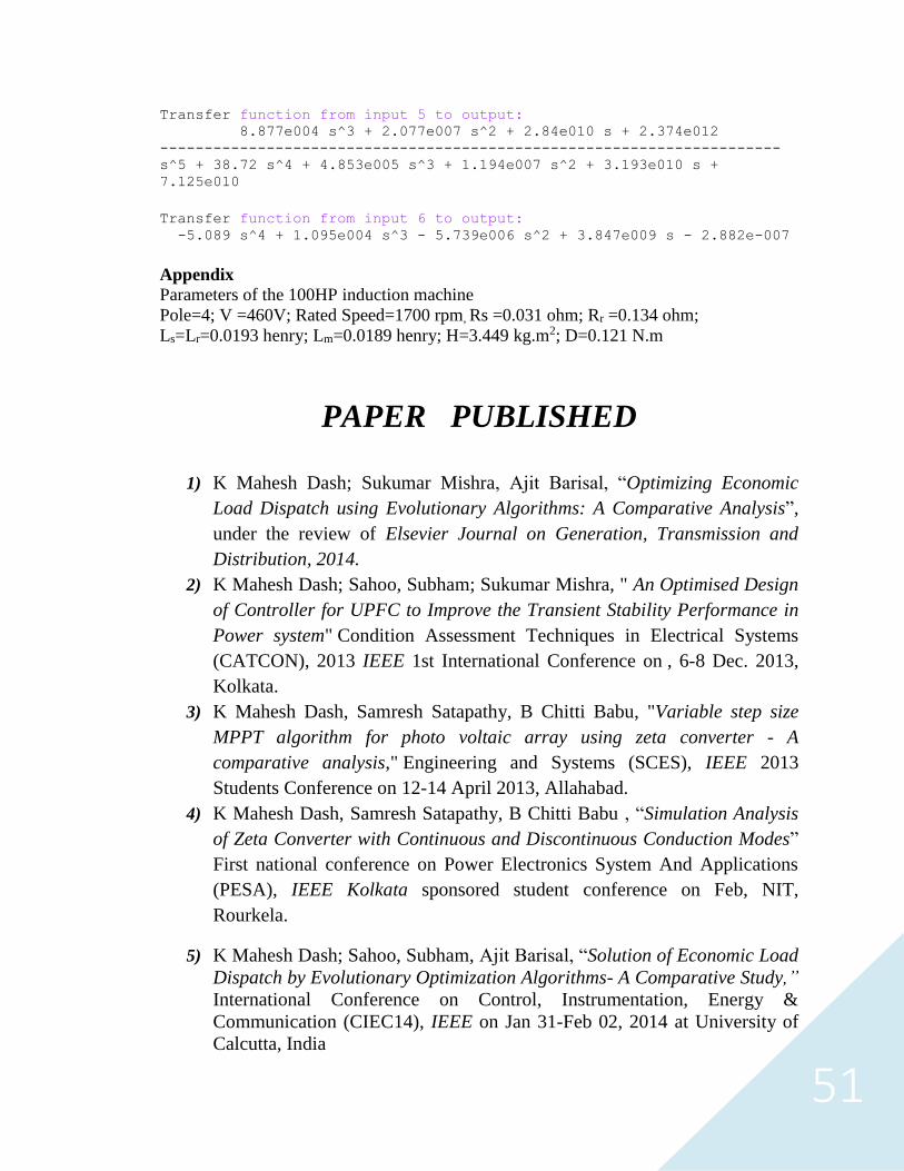
Transfer function from input 5 to output: 8.877e004 s^3 + 2.077e007 s^2 + 2.84e010 s + 2.374e012 ---------------------------------------------------------------------- s^5 + 38.72 s^4 + 4.853e005 s^3 + 1.194e007 s^2 + 3.193e010 s +

7.125e010

Transfer function from input 6 to output: -5.089 s^4 + 1.095e004 s^3 - 5.739e006 s^2 + 3.847e009 s - 2.882e-007

Appendix

Parameters of the 100HP induction machine

Pole=4; V =460V; Rated Speed=1700 rpm, Rs =0.031 ohm; Rr =0.134 ohm;

Ls=Lr=0.0193 henry; Lm=0.0189 henry; H=3.449 kg.m2; D=0.121 N.m

PAPER PUBLISHED

1) K Mahesh Dash; Sukumar Mishra, Ajit Barisal, “Optimizing Economic

Load Dispatch using Evolutionary Algorithms: A Comparative Analysis”,

under the review of Elsevier Journal on Generation, Transmission and

Distribution, 2014.

2) K Mahesh Dash; Sahoo, Subham; Sukumar Mishra, " An Optimised Design

of Controller for UPFC to Improve the Transient Stability Performance in

Power system" Condition Assessment Techniques in Electrical Systems

(CATCON), 2013 IEEE 1st International Conference on , 6-8 Dec. 2013,

Kolkata.

3) K Mahesh Dash, Samresh Satapathy, B Chitti Babu, "Variable step size

MPPT algorithm for photo voltaic array using zeta converter - A

comparative analysis," Engineering and Systems (SCES), IEEE 2013

Students Conference on 12-14 April 2013, Allahabad.

4) K Mahesh Dash, Samresh Satapathy, B Chitti Babu , “Simulation Analysis

of Zeta Converter with Continuous and Discontinuous Conduction Modes”

First national conference on Power Electronics System And Applications

(PESA), IEEE Kolkata sponsored student conference on Feb, NIT,

Rourkela.

5) K Mahesh Dash; Sahoo, Subham, Ajit Barisal, “Solution of Economic Load

Dispatch by Evolutionary Optimization Algorithms- A Comparative Study,”

International Conference on Control, Instrumentation, Energy &

Communication (CIEC14), IEEE on Jan 31-Feb 02, 2014 at University of

Calcutta, India

52