K.S.R.M. COLLEGE OF ENGINEERING,KADAPA.

B. VENKATA RAMUDU G. RAVI CHANDRA PALE-Mail : ramu_305398@yahoo.com E-mail : gandhamravi_g@ yahoo.co.inIII B.Tech. (E.E.E III B.Tech. (E.E.E.)K.S.R.M.C.E, Kadapa K.S.R.M.C.E, Kadapa

TOPIC

DIGITAL LOAD FREQUENCY CONTROL FORINTERCONNECTED POWER SYSTEMS

ABSTRACTThis paper reports on the advanced techniques of digital load frequency

control (LFC) for an interconnected power system under unknown deterministicpower demand. The authors observe that the predominant problem of LFC isresident in the low frequency domain associated with bulk generation change.This problem is highly influenced by limited generation response capability.Moreover, the load supplied by an interconnected power system is muchdependent on consumers and hence the amount of load to be servedinterconnected power system is much dependent on consumers and hence theamount of load to be served at a particulars time instant remains unknown tothe system. Therefore, the LFC is to be formulated as a tracking problemwhere the central role is played by energy source dynamics and the systemload following. This paper describe how the regulation of inter-area power flowscan effectively be improved by proper a user-friendly digital simulator whichsimulates the operation of load frequency controller of a three are closed andopen delta connected power system.

1

INTRODUCTION:

In recent years, rapid technological advancement has immensely increased theuse of electricity in agricultural, industrial, domestic and many other areas, notonly in the developed countries but in the developing countries of the world aswell. The raising demand for electricity has led to the formation of large andcomplicated interconnected power systems where various utilities or area s areconnected over long distance transmission lines, such that they can shareamong themselves their spinning reserve capacities during emergencies andcan take advantage of load diversity for economy of operation. It has beenfound in recent times as power demand is increasing rapidly, the generatingcapacities of the power stations are becoming inadequate for meeting thedemand. Under these circumstances, interconnection of the utilities becomesthe only solution as this, at first, helps to cater for the rising load demandwithout going for enhancement of generating capacities of the power stationsand secondly improves system reliability.

However, interconnected power systems face several operationalproblems as far as sudden load disturbances and faults are concerned. Theinterconnection of neighboring utilities increases the possibility of a healthy areagetting affected by the faults or disturbances taking place in another remote areand disturbance occurring in one area may endanger the stability of the otherareas if the source of disturbance is not quickly located and isolated from therest of the system. Keeping this in view, the power system engineers havefocused their attention on load frequency control (LFC) problem of theinterconnected power systems. During large disturbances or generation shifts,the security constraints or tie-line schedule changes are accommodated givingdue importance to the bulk power flows across potential separation boundarieswithin the network and it is the main purpose of LFC to restore the originalfrequency boundaries within the network and it is the main purpose of LFC torestore the original frequency and tie-line power flows in the system followingthe disturbance by effectively changing the generation of the affected area. Inorder to make the economic dispatch effective, the area generation requirementmust be established by quick execution of the essential function of LFC,. TheLFC is also to provide load tracking capability for the security of power supplyto the load, with persistent changes with the rapid and sustained variationswhich occur during certain periods of normal operation.

2

Linear optimal theory to the LFC has been widely applied to tackle thedamping of inter- area synchronizing swings. But in large interconnected powersystems the predominant problem of LFC resides in lower frequency domainassociated with very large generation change having limited generationresponse capability. In this paper, the authors describe the advance techniquesof digital load frequency control for multiple area interconnected power systemusing PI controllers with giving importance to optimal load tracking approach toLFC with dynamic limitations of thermal power plants including power flowreputation in the presence of immeasurable, sustained load changes.

LOAD FREQUENCY CONTROL PROBLEM

Classical Approach of LFC

The classical approach of regulation function is the concept of tie-line basiscontrol and this is applied for most modern interconnected systems. The tie-linebias control attempts to minimize its area control error (ACE) defined asfollows.

ACE1 = Pied +Bi Fi

The execution of tie- line bias control has the following aspects.

(i) each area regularities its own ACE leading to the overall objectiveof the regulation of the interconnected system, and

(ii) each area can achieve its assigned subtotal of regulating its ACEwithout some sort of inter-area coordination.

It is clear from this point of view that the first aspect can establish thedesired steady-state frequency and tie-line power flows whereas in thesecond aspect the integral control of ACE within each area leads to astable structure with the desired system equilibrium.

Linear Optimal Approach of LFC

The modern control techniques of linear optimal approach to thisproblem incorporate the dynamic aspects LFC. This linear optimal theory

3

is applied to obtain the desired operating state from any perturbed stateunder contingencies. In this formulation, several assumptions becomeimplicit leading to significant effects on the resultant controller.

(i) in the steady-state the system is quite capable to reduce thefrequency errors and the tie-line power flow errors to zero.

(ii) The power demand can be measured directly and

(iii) No constraint is imposed on the power plant other than thegovernment – turbine dynamics.

The aforesaid assumptions indicate that each area is quite capable ofmeeting a specific generation requirement. It is clear that an adequaterange of automatically controlled generation is available in each area forsatisfying the above requirement. Several contingencies, for example,loss of generation tie-line outage, failure in telemetering etc, mayprevent an area to meet its generation obligation. Mention must bemade that the desired steady-state with zero frequency error and zerotie-line flow error cannot be obtained unless each area can meet itsgeneration obligation. It leads to the persistence of abnormal steady-state which is deviated from the normal steady-state. The Fosha –Legend controller can take care of such abnormal situations with thehelp relative weighting parameters in the cost functional.

Since the power demand is not directly measurable, it has significantimpact on the results. The frequency error integrals and tie-lien powererror integrals are outputs and hence they must be driven to zero toachieve the appropriate steady state. Moreover, there is a constraint onthe rate of change of generation for large sustained changes irrespectiveof the type of generation. Sometimes these constraints can dominate theproblem of regulation. Even during normal operation. Manual generationrescheduling may be necessary by system operators during the period ofrapid load-change. This will lead to performance degradation due to theinability of direct measurement of power. Therefore, the power demandestimation is necessary to be incorporated into the controller as aprimary aspect of regulation.

4

The recent application of the optimal regulator theory of LFC has givenprime importance to the dynamic of power system regulation. Thepotentialistic of the approach have been investigated in earlier works butthe following two aspects of LFC should be properly addressed:

POWER SYSTEM INTERCONNECTION

Interconnection between power utilities or areas fro an importantpart of the overall power system and they contribute greatly to increasereliability of supply and economy of power production. In order to studypower production. In order to study power system dynamic under variousdisturbance conditions, it is desirable to model an interconnected powersystem as the importance and application of microcomputers have beengrowing continuously. In this paper, the authors have developed a digitala digital simulator for load frequency controller in order to study thebehaviour of a three area closed and open delta connected systemsunder different contingency conditions.

As area is a power system utility consisting of coherent genitors, whosegeneration must absorb its own load changes. An area is characterizedits combined governing characteristic shown in Fig. 1.

GENERATION (G) IN MW ---------- >Fig 1 Area combined governing characteristic

Steady –state curve that relate area frequency and total generation forchanges in area load. Each charastristics includes variation of area loadwith frequency as well as droop introduced by the combined effects of

5

all the governors on the prime movers for any change in frequency inthe area can be restored with the help of supplementary regulation. I.e.,the curve can be shifted vertically upwards with the same slope whichrepresents the combined effects of pulsing the speed changers of theprime movers within the area. The inverse slope changers of the primemovers within the area. The inverse slope of this curve is calledgovernor regulation and designated R (MW/Hz) and this slope plays animportant role in the steady state and dynamic behaviour o the tie-linecontrollers.

The area connections are shown in Fig. 2 Area # 1 is connected to Area#2 , Area #2 to Area # 3 and Area #3 to area #1 via tile lines. Theoutside arrows along with the tie-lines in Fig. 2. represent scheduledpower interchange at normal frequency. This rigid schedule is disturbed.However ,when a sudden increase in local occurs, for example, in Area#3. since alternator speed cannot change instantly, the load increase isinitially supplied out of the stored kinetic energy of the rotors of all theturbolternators in the three areas resulting in a droop of speed withcorresponding reduction in the system frequency. The governors in eachare them increase are generation of this lower frequency by shifting thearea combined characteristic GC1 to GC 2 as shown shares theincreased load in Area # 3 but at al lower system frequency. To restorethe normal system frequency and to increase the generation only in Area# 3 for accommodating its rise in load, a tie-line bias controller whichrespond to a typical tie-line bias characteristic is shown Fig 3.

The steady – state, linear tie-line bias characteristic of Fig3 relates arefrequency to area net tie-line interchange. P. Net tie-line powerinterchange into the area is considered negative and out of the area,positive. The bias B(MH/Hz) is defined is the inverse slope of this curveand t is and it is arbitrary ie., it can be made equal to smaller or longerthan the area governing regulation R. Each area controller must avail thedata leading to prevailing frequency (F1) and prevailing net interchange(PP) . These data are monitored and transmitted to each controller fromthe area tie-lines. Therefore, all three area

6

Controller know the scheduled net interchange at normal frequency foreach area as shown in Fig 2.AREA #1 AREA#2 AREA#3

P03Po ( Area #1) = Po1 – Po3Po (Area #2) = Po2 – Po1Po (Area #3) = Po3 – Po2

At prevailing frequency (F1 Hz) each controller can calculate prevailingnet interchange for each area as shown in Fig. 2.

PP 1 (Area #1) = P12 – P31PP1 (Area#2) = P23 –P12PP1 (Area #3) = P31– {23

With a bias value as per Fig. 3 each area can then calculate its ownarea requirement or the ACE as given below:

ACE = (Po– PP1) + (P1-P0) + (P1- P0) = P+BF

Where

B = [B]P = P0 – PP1

F = FB – F1

in the above equation, P is the deviation of net interchange from thenormal frequency schedule and B F is the automatic shift of theinterchange schedule with frequency. If the area requirement is positive

P31L1

L3P23

L2

P01P02

P12

7

or negative, the area controller with the help of supplementary regulationcommand will increase or decrease, respectively, the generation in itsarea by an amount of ACE megawatts.

When the system is operating at a normal frequency (F0), regardless, fthe value of the controller bias, the net interchange of tie-line power ofeach area remains on schedule, P0. each area requirement remainszero and each controller remains inoperative. If the value of each areacontroller bias (B) of Fig 2 is made equal to the value of its areagoverning regulation ® for a load increase in Area #2 becomes equal tothe biased scheduled interchange P1. the controllers for all of these areado not change area generations since their area requirements remainzero. However, the net interchange requirement remain(PP1) of Area #3as shown in Fig3, deviates from the bias schedule (P1). Therefore, thecorresponding tie-line bias controller increase generation in Area #3 ,with supplementary regulation command, by ACE mega walls whichequals the load increase the thus the system restores its normalscheduled frequency.

If the value of each controller bias his made greater or smaller than thevalue of its area regulation, then the Areas #1 and #2 initially contributemore or less than their normal share of the load increase in Area #3 andthe system frequency drop less or more severely than the of theprevious case. The end result in steady-state. However , is that Area #3absorbs its own increase of loads at normal frequency by increasing thearea generation.

In case of any contingency , the operation of the load frequencycontroller should be such that the power system must regain its stablecondition with respect to the quality of power within a few seconds.

DEVEOPMENT OF DIGITAL SIMULLATOR

Block Diagram Representation of Three Area interconnected powersystem.

The digital simulator of the typical three area closed delta connectedpower system is represented by a block diagram as shown in the Fig. 4,it is clear from the figure that each area has its own control on its

8

operation there are three main blocks, namely, speed governor , turbineand power system. In this respect, each area s assumed to be similarand hence the time constants of the aforesaid blocks for all the areasfare taken to be 0.88 sec. 0.3 sec, respectively. Rigorous study hasbeen done with different areas having different time constants of theseblocks. A P1 controller is incorporated in each block for obtaining zerosteady – state error for the deviations of both the system frequency andtie-line power. The constants (i) frequency bias constant and (ii) areagoverning regulation are kept different for different areas. Thus the areasbecome different in their performances. The implementation of thecalculation of tie-line powers is done with several blocks as shown in thefigure, Provision has also been make for the display of the followingcharacteristic of all the areas (i) tie-line power flow deviation and (ii) areafrequency with one tie-line delinked as shown in the block diagrammaticrepresentation of Fig. 5. The performance of this open delta powersystem is a bit worse than the delta-connected one, Bu in case of anycontingency the steady state of the system can be regained withoutentering into emergency zone. The deviations in that case are a bit morethan the previous one resulting in the requirement of more time torestore the original steady – state.

Algorithm For Simulator

The simulator package has been implemented for simulating theoperation of four multi-area power systems with different configurations,

9

both with and without the load frequency controller. The programs havebeen developed through M-files in MATLAB version 4.2 c1 in theenvorinment of Microsoft Windows 95. the simulator has been madeextensively interactive, graphic – oriented and user friendly. Thealgorithm is as follows.

(i) initialize the graphic window on the VDU screen,(ii) set the parameters start time, stop time, minimum and maximum

time step sizes and relative error for solving the systemdifferential equations using Runge- Kutta method.

(iii) Draw ‘power system’ transfer function block for Area # 1 withtransfer function form Gp1 (s) ,

(iv) Set the default values of the coefficients of the numerator anddenominator polynomials of GP1(s).

(v) Draw ‘turbine ‘ transfer function block for Area # 1 with transferfunction of the form GT1 (s) = kn /(1+stn) .

(vi) set the default values of the coefficients of the numerator anddenominator polynomials of GT1(s),

(vii) draw 'Speed Governor' transfer function block [or Area #1 with transferfunction of the form GG1 (s) =, KG1/(1 + sT(G1),

(viii) set the default values of the coefficients of the numerator anddenominator polynomials of GG1(s).

(ix) connect the output o[ the' Speed Governor' block 10 (he input of the'Turbine' block to realise the combined transfer function GUT! (s) asshown in Fig 4-7,

10

(x) draw 'PI Controller' transfer function block for Area ill with transferfunction of the form (k1 + k2/s) = (sk1 + k2)/s.. The values of k1 and k2should be with in 0 and 1.0,

(xi) set the default values of the coefficients of the numerator anddenominator polynomials of the transfer function of 'PI Controller',

(xii) draw the gain block B1 for representing frequency bias constantparameter for Area #1 and set its default value, The value of frequencybias constant should be within 0 and 1.0,

(xiii) draw the gain block '1/Rl' for representing the reciprocal of areagoverning regulation for Area #1 and set its default value,

(xiv) draw the step function block PD1' for representing step load input 10Area It I. the value of PD1should preferably be within 0 and 1.0 pu,

(xv) provide option for pointing any block by moving the cursor with the helpof the mouse in order to change the default system and controlparameters through keyboard and/or mouse. It should be I noted that:my parameter can be assigned the realistic values as per any (lowerplant as obtained. There is no limit for setting the values of theparameters, but in order to get actual responses, values arc to beassigned to the parameters around the realistic ones, repeat steps (iii),to(x v) for Area #2,

(xvii) repeat steps (iii) to (xv) for Area ft3,(xviii) draw the gain blocks for representing the '2p T ij

o parameter for thetransmission lines connecting the j-th area,

(xix) draw the required summer and integrator blocks for realizing the blockdiagram of Fig 4-7,

(xx) connect all the blocks with straight line connectors as per the blockinterconnect shown in Fig 4-7.

(xxi) set the names of (he output data files for storing a1l , the timerc.sJ1CJOses for the deviations of area

frequencies, area tic powers and tie -line power flows,(xxii) input the step load change magnitude(s) for one or more area(s),(xxiii) calculate the aforesaid time responses in the form of output parameters,

and(xxiv) store the output parameters in the corresponding output data files.Main Features of Simulator PackageThe main features of all the aforesaid four programs arc discussed thus.In the program, the system configuration is represented as a block diagram.

Each of the power system modules like speed governor, turbine, thecontroller and the control area designated as power system in the

11

programs, are mathematically represented by simple algebraic first ordertransfer functions consisting of a single gain factor and a single timeconstant.

The controller for each control area has been modeled for proportional plusintegral control using transfer functions of the form (k1+k2/s) with a negativefeedback. The individual blocks are interconnected using other blocks likesummer, integrator, sample gain factors and line connectors for realizing theblock diagrams.

All the three control strategies, for example (a) flat frequency control (b)flat tie-line control and (c) tie-line bias control can be accomplished by minormodifications in the programs.

Display of Output parametersThe program calculates the output parameters, namely, the time responses ofthe following:

(i) system frequency deviations f1. f2 and f3 (in Hz)

(ii) area tie- power deviations P tie, 1, P tie, 2 and Ptie 3 ( in pu

MW with respect to area capacity) for the three areas, Area#1,

Area#2 and Area#3 , respectively,

(iii) power flow deviation P tie1,2 ( in pu MW) in the tie-line between

Area #1 and Area#2.

(iv) Power flow deviation P tie23 (pu MW) in the tie-line between

Area #2 and Area #3. and

(v) Power flow deviation P tie 31 (in pu MW) in the tie-line between

Area #3 and Area#1 (only in case of closed delta connected

system )

As per convention, the tie- power flowing out from an area is considered

positive and that flowing into an area is taken to be negative. Tie – line powers

flowing from Area #1 to Area #2 from Area#2 to Area #3 and from Area #3 to

12

Area #1 are taken to be positive and the opposite directions are considered

negative

ANALYSIS OF RESULT OF SIMULATOR

All the studies have been performed on both the closed delta and open

delta configurations of the interconnected power system. The performance of

both the systems are almost similarly except the fact that in the open delta

configuration, the system takes a bit more time to restore its steady state

condition after the incidence of any contingency in the system. The cases are

as follows:

(i) any area loaded by a step load of 0.52 pu.

(ii) Any two areas loaded by a step load of 0.25 pu each,

(iii) All the three areas loaded by a step load of 0.25 pu each

(iv) Any two areas unloaded by an amount of 0.25 pu in one step and

All the three areas unloaded by an amount of 0.25 pu in one step.

13

Fig 6 (a) shows the deviation of frequency of each area and restorationof the original system frequency during a step loading of 0.25 pu to Area# 2 it indicates that the frequency of the concerned area is affectedmore than the others in the transient period. In this case the deviation oftie-powers of each area is shown in Fig 6 (b). Here also the tie-power ofthe concerned area is affected a bit more. Moreover, the deviation of tie-powers of the other areas are in the opposite direction to that of theArea #2 it is clear from both the figures that the system set point isregained within 10 min after the step loading.

14

15

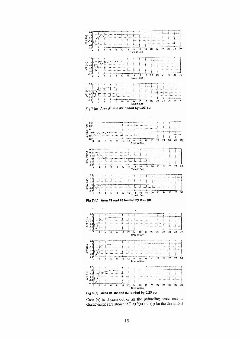
Similar observations are made in Figs 7 (a) and (b) with the secondcase when Area #1 and #3 are loaded by a step load of 0.25 pu each.Here also, the concerned areas are affected in a similar manner unlikethe unloaded one. But the amount of deviations is more in this case thanthe previous one.

In case (iii) all the areas are simultaneously loaded with a step load of0.25 pu each. The deviation of frequency and tie-power characteristicsare shown in Figs 8 (a) and (b) , respectively. In this case the tie-powerof Area #1 is least deviated lively. In this case the tie-power of Area #2and Area #3 are deviated in the directions opposite to each other.Moreover, the setting time is around 14 sec.

16

17

Since the characteristic of all the cases for open delta configuration aresimilar to that of closed delta system, the characteristics of its typicalcase of loading of all the three areas by a step load of 0.25 pu each areshown in Figs 10 (a) and (b) . here the system restoration is bit sluggish.

CONSCLUSION

This paper reports in detail the advanced digital control ofinterconnected power system having performed rigours testing on atypical interconnected power system with the aid of digital simulator. Inthe mathematical modeling part of the digital simulator, the authors haveused both classical and state variable approach of digital simulation. Theresults obtained from this simulator bear a close similarity to a practical

18

interconnected power system. In the view of the authors, though theperformance of open delta connected power system is slightly sluggishstill its performance is satisfactory subject to the reliability and quality ofpower supplied to the consumer’s premises. Mention must be make thatthe closed delta configuration always better than the open delta onethough the open delta configuration is much stable in its performance.Since the state variable approach is appropriate to the state – of – the– art requirement of interconnected power system. The author suggestthis approach to be more acceptable. This simulator is advantageous inthe implementation of any kind of modern control strategy with slightesteffort. The software developed for this simulator is flexible and userfriendly with sufficient interactive graphical interface. Hence it does notimpose any hindrance to the non-experts of this software for itsimmense application in the simulation study of any interconnected powersystem.

REFERENCES:1. C.E. Fosha and O.I. Elgend. “ The Megawatt Frequency Control

problem Anew Approach via Optimal control Theory ‘ IEEETransactions, via PAS – 89 no 4, 1970 p 563.

2. M.S. Calovic’ Linear Regulator Design for a Load and FrequencyControl’ ibid vol PAS –91 no 6,m1972 p 2271.

3. S.M. Miniesy and E.V. Bohn ‘ Optimal Load Frequency Continuouscontrol with Unknown Determinstic power Demand ibid no. 5,1972 p1910.

4. N.N. Benjamin and W.C. Chan ‘ Multilevel Load- Frequency Controlof Interconnected Power System ibid no 3, 1978 p 521.

5. A. Bose and 1 Atiyyah ‘ Regulation Error in Load Frequency Controlibid, vol PAS 99, March/April 1989, p 650.

END

19

20