The supplementary document of “LLR: A latent

low-rank approach to colocalizing genetic risk variants

in multiple GWAS”

Jin Liu∗1, Xiang Wan∗2, Chaolong Wang3, Chao Yang4, Xiaowei Zhou5, and Can Yang†6

1Center of Quantitative Medicine, Duke-NUS Graduate Medical School, Singapore2Department of Computer Science, Hong Kong Baptist University, Hong Kong, China

3Genome Institute of Singapore, A∗STAR, Singapore4Baidu Inc., Shanghai, China

5Computer and Information Science, University of Pennsylvania, USA6Department of Mathematics, Hong Kong University of Science and Technology, Hong

Kong, China

July 9, 2017

1 Details of derivation of likelihood function

The marginalization of equation (5) in the main article can be written as

Pr(Zlk) = Pr(Zlk, ηlk = 1) + Pr(Zlk, ηlk = 0). (S1)

Now we can derive the marginalization over this partition. The first part is

Pr(Zlk, ηlk = 1)

=Pr(ηlk = 1)∑γlk

Pr(Zlk,γlk|ηlk = 1))

=Pr(ηlk = 1)

Ml∑j=1

Pr(Zlk|γlk(j = 1))Pr(γlk(j = 1)|ηlk = 1))

=πk

Ml∑j=1

1

MlPr(Zlk|γlk(j = 1)),

(S2)

∗Joint first author†Correspondence author

1

where Pr(Zlk|γlk(j = 1)) = N(Σl[λlk γlk(j = 1)],Σl

)and Pr(γlk(j = 1)|ηlk = 1)) = 1

Ml(non-

informative prior over Ml configurations of γlk). Note that the second equality holds because we

assumed only one risk SNP in locus l.

The second part is

Pr(Zlk, ηlk = 0)

=Pr(ηlk = 0)Pr(Zlk|γlk = 0)Pr(γlk = 0|ηlk = 0))

=(1− πk)Pr(Zlk|γlk = 0),

(S3)

where Pr(Zlk|γlk = 0) = N (0,Σl) and Pr(γlk = 0|ηlk = 0)) = 1.

Combination of Equations (S2) and (S3) gives Equation (6) in the main article.

2 The theoretical justification of the EM-path algorithm

In this section, we justify our EM-path algorithm by characterizing the update in M-step as steepest

descent such that the ascent condition holds during the EM iterations. Consider the part of the

logistic log-likelihood function in the Q function at the t-th iteration

f(X,x0) =

K∑k=1

L∑l=1

EΘ(t) [ηlk|Z] log πlk + EΘ(t) [1− ηlk|Z] log(1− πlk)

.

The first order Taylor approximation of f(X + W,x0 + w0) is

f(X + W,x0 + w0) ≈ f(X + W,x0 + w0) = f(X,x0) + tr(W>G(t)) + w>0 g(t). (S4)

Since tr(W>G(t)) and w>0 g(t) are linear in W and w0, respectively, f(X+W,x0+w0) can be made

as positive as possible by taking W and w0 large. To make the optimization problem sensible, the

steepest ascent method restricts the norm of W and w0. Let ‖ · ‖m and ‖ · ‖v be any matrix and

vector norms, respectively. The steepest ascent direction is given as

(∆,∆0) = arg maxW,w0

tr(W>G(t)) + w>0 g(t), subject to ‖W‖m ≤ 1, ‖w0‖v ≤ 1, (S5)

2

With the ascent direction, X and x0 can be updated as

X = X + ε∆,

x0 = x0 + ε∆0,(S6)

where ε is the step size. Typically, the step size ε can be chosen by line search. For our applica-

tion, we tried ε = 0.1, 0.05, 0.01, 0.005, 0.001 and find that the choice of step size ε is intensive to

estimation of posterior probabilities Pr(ηlk = 1|Z) and Pr(ηlk = 1,γlk(j = 1)|Z). In our simulation

and real data analysis, we simply set ε = 0.05. We noticed some other strategies for tuning the

step size are available in [? ].

In our case, we consider the nuclear norm ‖ · ‖∗ for matrices and the L2 norm ‖ · ‖2 for vectors.

Hence optimization problem (S5) becomes

(∆,∆0) = arg maxW,w0

tr(W>G(t)) + w>0 g(t), subject to ‖W‖∗ ≤ 1, ‖w0‖2 ≤ 1, (S7)

Note that the updates for W and w0 are separable. We first consider optimization problem

∆ = arg maxW

tr(W>G(t)), subject to ‖W‖∗ ≤ 1.

Using the fact that the dual of the trace norm ‖W‖∗ is the spectral norm ‖W‖2, the closed form

solution is given as [? ] is given by

∆ = uv>, (S8)

with u, v being leading left and right singular vectors, respectively, of G(t). Notice that obtaining

leading singular vectors u and v is much cheaper than singular value decomposition. Clearly, v is

given by the leading eigenvector of [G(t)]TG(t) which is a K ×K matrix, where K is the number

of studies and is much smaller than the number of loci L. Then u = Gv/‖Gv‖2.

Similarly for the intercepts, the optimal solution for 40 can be written as

∆0 = εg(t)

‖g(t)‖2. (S9)

3

Since the steepest accent method ensures the ascent condition Q(Θ(t+1); Θ(t)) ≥ Q(Θ(t); Θ(t)),

we can guarantee the convergence of the EM-path algorithm. For completeness, we summarize the

EM-path algorithm in Algorithm 1.

Algorithm 1: The proposed EM-path Algorithm)

Parameters: Θ = x0,XInitialize x

(0)0 using separate models on each trait k and X(0) = 0.

for t = 1, 2, . . . , t, . . . , T doE-step:update posterior of γ and η.M-step:

update x(t)0 and X(t) using (S6).

end

3 More details about cross validation

For ten-fold cross validation, we randomly partition L×K entries in η into five folds with roughly

equal sizes, Ω1, . . . ,Ω5, such that Ω1 ∪ · · · ∪ Ω5 = Ω and Ω1 ∩ · · · ∩ Ω5 = ∅. For the first around,

denote the training index as Ωtrain1 = Ω1 ∪ · · · ∪Ω4 and Ωtest1 = Ω5. The overall incomplete-data

log-likelihood

`p(Θ) =K∑k=1

L∑l=1

log

(1− πlk)N (0,Σl)

+ πlk

[ Ml∑j=1

1

MlN(Σl[λlk γlk(j = 1)],Σl

)],

(S10)

should be modified for training as

`p(Θ) =∑

(l,k)∈Ωtrain1

log

(1− πlk)N (0,Σl)

+ πlk

[ Ml∑j=1

1

MlN(Σl[λlk γlk(j = 1)],Σl

)].

(S11)

4

Accordingly, log-likelihood on the testing data is given as

`p(Θ) =∑

(l,k)∈Ωtest1

log

(1− πlk)N (0,Σl)

+ πlk

[ Ml∑j=1

1

MlN(Σl[λlk γlk(j = 1)],Σl

)].

(S12)

Indeed, this is the cross-validation strategy often used in matrix completion, e.g., [? ].

4 More results in the simulation experiment.

In this section, we present more simulation results.

5

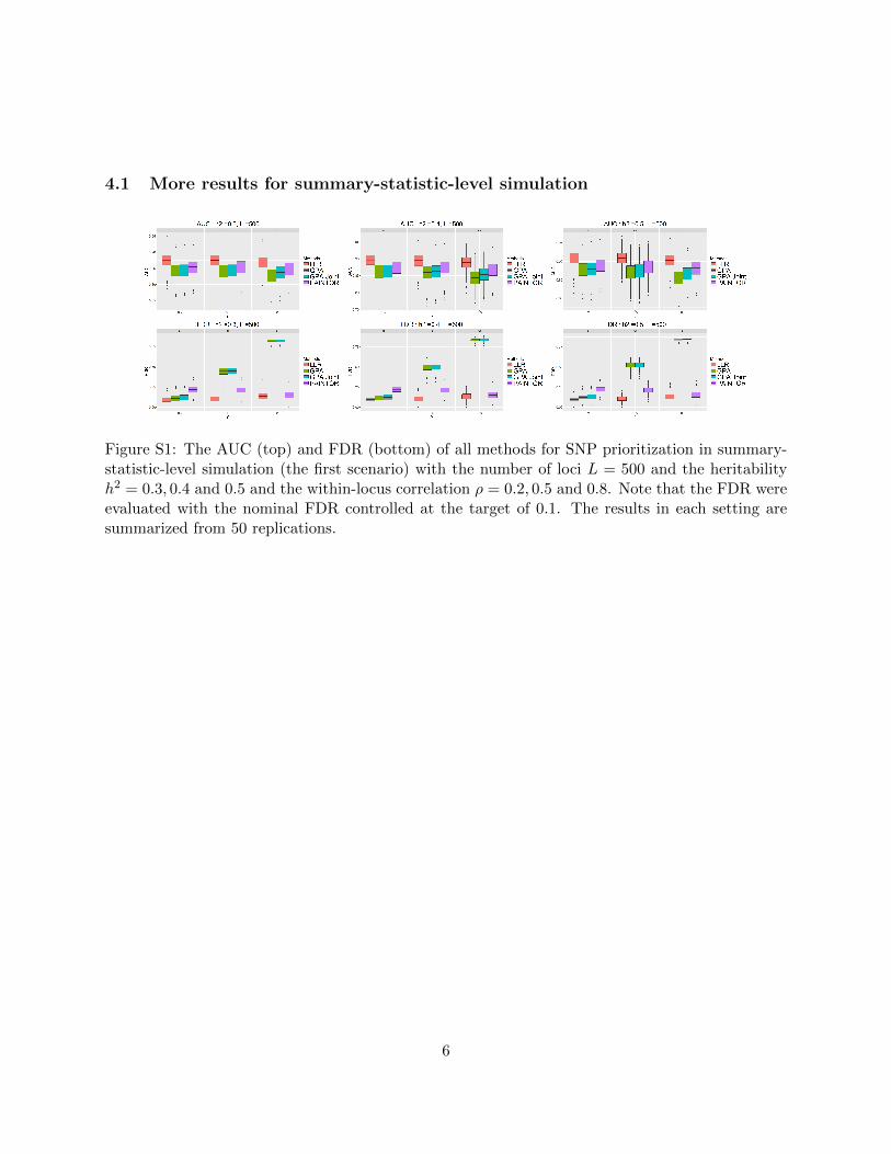
4.1 More results for summary-statistic-level simulation

Figure S1: The AUC (top) and FDR (bottom) of all methods for SNP prioritization in summary-statistic-level simulation (the first scenario) with the number of loci L = 500 and the heritabilityh2 = 0.3, 0.4 and 0.5 and the within-locus correlation ρ = 0.2, 0.5 and 0.8. Note that the FDR wereevaluated with the nominal FDR controlled at the target of 0.1. The results in each setting aresummarized from 50 replications.

6

Figure S2: The AUC (top) and FDR (bottom) of all methods for SNP prioritization in summary-statistic-level simulation (the first scenario) with the number of loci L = 2, 000, the heritabilityh2 = 0.3, 0.4 and 0.5 and the within-locus correlation ρ = 0.2, 0.5 and 0.8. Note that the FDR wereevaluated with the nominal FDR controlled at the target of 0.1. The results in each setting aresummarized from 50 replications.

7

4.2 The performance for individual-level simulation

Figure S3: Performance comparison of LLR, GPA, GPA-Joint and PAINTOR (individual-levelsimulation) with the number of loci L = 500 (left panel) and L = 2000 (right panel). In each panel,the four methods are tested with heritability h2 = 0.3, 0.4, and 0.5, and within-locus correlationρ = 0.2, 0.5, and 0.8. The results in each setting are summarized from 50 replications.

Figure S4: The AUC (top) and FDR (bottom) of all methods for SNP prioritization in individual-level simulation (the second scenario) at the number of loci L = 500 and the heritability h2 = 0.3, 0.4and 0.5 and within-locus correlation ρ = 0.2, 0.5 and 0.8. Note that the FDR were evaluated whenthe nominal FDR was controlled at the target of 0.1. The results in each setting are summarizedfrom 50 replications.

8

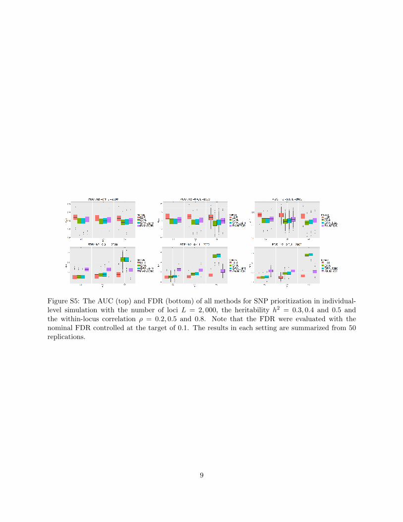
Figure S5: The AUC (top) and FDR (bottom) of all methods for SNP prioritization in individual-level simulation with the number of loci L = 2, 000, the heritability h2 = 0.3, 0.4 and 0.5 andthe within-locus correlation ρ = 0.2, 0.5 and 0.8. Note that the FDR were evaluated with thenominal FDR controlled at the target of 0.1. The results in each setting are summarized from 50replications.

9

4.3 The performance on data sets with no pleiotropy

Figure S6: The AUC (top) and FDR (bottom) of Sep (separate analysis) and LLR for SNP priori-tization accuracy using data sets with no pleiotropy at the number of loci L = 500, the heritabilityh2 = 0.3, 0.4 and 0.5 and within-locus correlation ρ = 0.2, 0.5 and 0.8. Note that the FDR wereevaluated with the nominal FDR controlled at the target of 0.1. The results are based on 50simulations.

Figure S7: The AUC (top) and FDR (bottom) of Sep (separate analysis) and LLR for SNP prioriti-zation accuracy using data sets with no pleiotropy at the number of loci L = 2000, the heritabilityh2 = 0.3, 0.4 and 0.5 and within-locus correlation ρ = 0.2, 0.5 and 0.8. Note that the FDR wereevaluated with the nominal FDR controlled at the target of 0.1. The results are based on 50simulations.

4.4 The performance on the locus level

Figure S8: The AUC (top) and FDR (bottom) of Sep (separated analysis) and LLR for locusprioritization using summary data at the number of loci L = 2, 000, the true NCP at ncp = 2.5, 3and 3.5 and within-locus correlation ρ = 0.2, 0.5 and 0.8. Note that the FDR were evaluated withthe nominal FDR controlled at the target of 0.1. The results are based on 50 simulations.

Figure S9: The AUC (top) and FDR (bottom) of Sep (separated analysis) and LLR for locusprioritization using genotype data at the number of loci L = 2, 000, the true NCP at ncp = 2.5, 3and 3.5 and within-locus correlation ρ = 0.2, 0.5 and 0.8. Note that the FDR were evaluated withthe nominal FDR controlled at the target of 0.1. The results are based on 50 simulations.

4.5 The performance using true NCP

4.5.1 SNP level

Figure S10: The AUC (top) and FDR (bottom) of Sep (separate analysis) and LLR using trueNCP for SNP prioritization accuracy using summary data at the number of loci L = 500, the trueNCP at ncp = 2.5, 3 and 3.5 and within-locus correlation ρ = 0.2, 0.5 and 0.8. Note that the FDRwere evaluated with the nominal FDR controlled at the target of 0.1. The results are based on 50simulations.

4.5.2 Locus level

Figure S11: The AUC (top) and FDR (bottom) of Sep (separated analysis) and LLR using trueNCP for SNP prioritization using summary data at the number of loci L = 2, 000, the true NCPat ncp = 2.5, 3 and 3.5 and within-locus correlation ρ = 0.2, 0.5 and 0.8. Note that the FDRwere evaluated with the nominal FDR controlled at the target of 0.1. The results are based on 50simulations.

Figure S12: The AUC (top) and FDR (bottom) of Sep (separate analysis) and LLR using trueNCP for locus prioritization accuracy using summary data at the number of loci L = 500, the trueNCP at ncp = 2.5, 3 and 3.5 and within-locus correlation ρ = 0.2, 0.5 and 0.8. Note that the FDRwere evaluated with the nominal FDR controlled at the target of 0.1. The results are based on 50simulations.

Figure S13: The AUC (top) and FDR (bottom) of Sep (separated analysis) and LLR using trueNCP for locus prioritization using summary data at the number of loci L = 2, 000, the true NCPat ncp = 2.5, 3 and 3.5 and within-locus correlation ρ = 0.2, 0.5 and 0.8. Note that the FDRwere evaluated with the nominal FDR controlled at the target of 0.1. The results are based on 50simulations.

Figure S14: The comparison of FDR under different thresholds (3.7, 4.6 and 5.3) in LLR.

4.5.3 Simulation study with different correlation structures

For the above simulation studies, we used autoregressive structure to simulate the correlation among

SNPs. We further evaluated our method under different correlation structures:

• Equal correlation matrix

Σ(j, k) =

1 if j = k,ρ if j 6= k.

(S13)

• Banded correlation matrix

Σ(j, k) =

1 if j = k,ρ if |j − k| = 1,ρ/2 if |j − k| = 2,0 otherwise.

(S14)

We varied parameter ρ ∈ 0.2, 0.4, 0.6 to mimic different levels of correlation among SNPs. The

results shown in Figures 4.5.3 and 4.5.3 indicate that the FDR of LLR can be controlled at nominal

level 0.1 with non centrality parameter 5.3 under different correlation structures.

Figure S15: The AUC (top) and FDR (bottom) of all methods for SNP prioritization in summary-statistic-level simulation with the number of loci L = 500 and the heritability h2 = 0.3, 0.4 and 0.5and the within-locus correlation ρ = 0.2, 0.4 and 0.6 under equal correlation structure. Note thatthe FDR were evaluated with the nominal FDR controlled at the target of 0.1. The results in eachsetting are summarized from 50 replications.

Figure S16: The AUC (top) and FDR (bottom) of all methods for SNP prioritization in summary-statistic-level simulation with the number of loci L = 500, the heritability h2 = 0.3, 0.4 and 0.5 andthe within-locus correlation ρ = 0.2, 0.4 and 0.6 under banded correlation structure. Note that theFDR were evaluated with the nominal FDR controlled at the target of 0.1. The results in eachsetting are summarized from 50 replications.

4.6 Comparison between the EM-path algorithm and the standard EM algo-rithm

Figure S17: The solution path from the EM path algorithm and the standard EM algorithm for asynthetic dataset.

Table S2 shows the timing comparison of the EM-path algorithm and the standard EM algorithm

under different choices of L and ρ. The solution paths of these two algorithms are shown in Figure

S17. From Figure S17, we can observe that the solution paths of these two algorithm are very similar

with each other. However, the EM-path algorithm runs about four times faster than standard EM

algorithm.

Table S1: Efficiency comparison of the EM-path algorithm and the standard EM algorithms solvingLLR.

L ρ EM boosting EM regularized

500 0.2 5.88 28.18500 0.5 5.40 26.04500 0.8 5.69 25.91

1000 0.2 11.68 53.831000 0.5 10.92 53.841000 0.8 12.22 54.941500 0.2 30.31 105.991500 0.5 27.73 104.481500 0.8 20.16 91.282000 0.2 50.90 163.462000 0.5 52.39 163.172000 0.8 43.87 151.92

5 Real data analysis

In this section, we provide more details about the real data analysis.

5.1 The details of the data sets

Table S2: GWAS data sets in our experimentID YEAR Traits LinkTAG cpd 2010 smoking http://www.med.unc.edu/pgc/downloads

IGAP 2013 Alzheimer’s disease http://www.pasteur-lille.fr/en/recherche/u744/igap/igap_download.php

GCAN 2014 anorexia nervosa http://www.med.unc.edu/pgc/files/resultfiles/gcan_meta-out.gz

cardiogram 2010 coronary artery disease http://www.cardiogramplusc4d.org/downloads/

FastingGlucose 2012 fasting glucose http://www.magicinvestigators.org/downloads/

SCZ 2011 Schizophrenia http://www.med.unc.edu/pgc/downloads

DHA 2011 plasma DHA http://www.chargeconsortium.com/main/results

MS 2013 multiple sclerosis https://www.immunobase.org/downloads/protected_data/iChip_Data/

Putamen 2015 human subcortical brain structures http://enigma.ini.usc.edu/wp-content/uploads/E2_EVIS/

BMI MEN 2013 body mass index of men https://www.broadinstitute.org/collaboration/giant/index.php/GIANT_consortium_data_files

BMI WOMEN 2013 body mass index of women https://www.broadinstitute.org/collaboration/giant/index.php/GIANT_consortium_data_files

PCV 2012 packed cell volume https://www.ebi.ac.uk/ega/studies/EGAS00000000132

T1D 2008 Type 1 Diabetes https://www.immunobase.org/page/Overview/display/study_id/GDXHsS00004

ADHD 2010 attention deficit-hyperactivity disorder http://www.med.unc.edu/pgc/downloads

MDD 2013 major depressive disorder http://www.med.unc.edu/pgc/downloads

Caudate 2015 human subcortical brain structures http://enigma.ini.usc.edu/wp-content/uploads/E2_EVIS/

BPD 2011 bipolar disorder http://www.med.unc.edu/pgc/downloads

ASD 2013 autism spectrum disorder http://www.med.unc.edu/pgc/downloads

5.2 Details on preprocessing the directions of Z-scores

Since the directions of Z-scores depend on the reference alleles that individual GWASs used, it is

not necessary that the reference panel data set from the 1000 Genome Project used the same set

reference alleles for all SNPs. Thus, we matched the reference alleles in each GWAS with the 1000

Genome reference panel data set. If they were the same, we kept the directions of corresponding Z-

scores. Otherwise, we changed the directions of Z-scores for the corresponding SNPs. In addition,

ambiguity may come from the fact that the reference alleles and non-reference alleles rely on whether

the starting points were from 3’ or 5’. Hence we removed these ambiguous SNPs.

5.3 More results in real data analysis

Figure S18: Manhattan plots of all 18 traits using LLR. The y-axis is − log10 fdrSNP

. Comparingwith Figure S19, it is clear that LLR can identified some variants whose signals are not strongenough to be selected by separated analyses. The numbers of significant hits under different FDRthreshold are given in Table S3 and Table S4.

Figure S19: Manhattan plots of all 18 traits using separate analyses. The y-axis is − log10 fdrSNP

.

Table S3: Number of Locus identified below different threshold for LLR and Sep (separate analysis)

Data Sets Local FDR threshold0.2 0.1 0.05

LLR Sep LLR Sep LLR Sep

TAG cpd 1 1 1 1 1 1

IGAP 35 18 32 13 23 12

GCAN 4 4 4 3 1 1

cardiogram 78 33 72 22 69 15

FastingGlucose 53 26 47 22 39 20

SCZ 72 23 64 13 55 9

DHA 2 2 2 1 1 1

MS 112 67 102 56 89 48

Putamen 5 5 4 4 4 4

BMI-MEN 35 22 31 16 28 13

BMI-WOMEN 39 26 32 20 28 17

PCV 53 21 46 20 38 14

T1D 147 72 129 58 115 49

ADHD 0 0 0 0 0 0

MDD 0 0 0 0 0 0

Caudate 1 1 1 1 1 1

BPD 5 5 4 3 2 2

ASD 2 2 2 2 1 1

Total 644 328 573 255 495 208

Table S4: Number of SNPs identified below different threshold for LLR and Sep (separate analysis)

Data Sets Local FDR threshold0.2 0.1 0.05

LLR Sep LLR Sep LLR Sep

TAG cpd 1 1 1 1 1 1

IGAP 9 7 6 3 4 3

GCAN 2 2 1 0 0 0

cardiogram 36 13 28 7 18 6

FastingGlucose 25 12 17 11 15 11

SCZ 25 7 14 5 10 2

DHA 0 0 0 0 0 0

MS 51 31 39 24 26 18

Putamen 2 2 2 2 1 1

BMI-MEN 5 1 1 0 1 0

BMI-WOMEN 7 4 4 2 2 1

PCV 26 13 18 9 7 5

T1D 63 38 42 30 33 27

ADHD 0 0 0 0 0 0

MDD 0 0 0 0 0 0

Caudate 0 0 0 0 0 0

BPD 1 1 0 0 0 0

ASD 0 0 0 0 0 0

Total 253 132 173 94 118 75

Table S5: New identified variants using LLRData Sets SNP id Chr Pos Type Gene

IGAP rs7812391 8 31121769 intergenic WRN(dist=90492),NRG1(dist=375499)rs3752240 19 1051214 exonic ABCA7rs6024881 20 55020689 intronic CASS4

GCAN rs923768 8 19530963 intronic CSGALNACT1cardiogram rs4675833 2 241947122 intronic SNED1

rs9866277 3 86105340 intronic CADM2rs1992265 4 44531665 intergenic KCTD8(dist=80841),YIPF7(dist=92689)rs6842241 4 148400819 intergenic TTC29(dist=533785),EDNRA(dist=1250)rs1533837 4 171644884 intergenic LINC01612(dist=440011),LOC100506122(dist=316869)rs2395656 6 36662171 intergenic CDKN1A(dist=7055),RAB44(dist=3457)rs1974369 6 73864494 intronic KCNQ5rs2096066 6 151255434 intronic MTHFD1Lrs1495741 8 18272881 intergenic NAT2(dist=14158),PSD3(dist=111932)rs7819541 8 22042151 intronic BMP1rs481294 9 27190890 intronic TEKrs505922 9 136149229 intronic ABO

rs10887650 10 88461699 intronic LDB3rs2297472 10 90984990 intronic LIPArs1180610 10 131859987 intergenic EBF3(dist=97896),LINC00959(dist=2175)rs6590202 11 126274032 intronic ST3GAL4rs11067009 12 114673596 intergenic RBM19(dist=269420),TBX5(dist=118139)rs4306376 13 107236514 intergenic ARGLU1(dist=16000),LINC00551(dist=33644)rs12873154 13 110920852 intronic COL4A1rs10520769 15 95382263 intergenic MCTP2(dist=355082),LOC440311(dist=16329)rs8111989 19 45809208 downstream CKM,MARK4

FastingGlucose rs1996546 4 185714289 intronic ACSL1rs926127 8 127320627 intergenic LINC00861(dist=357186),LOC101927657(dist=17113)

rs12370484 12 61844049 intergenic SLC16A7(dist=1660414),FAM19A2(dist=257980)rs7981007 12 133026146 intergenic LOC101928416(dist=117985),FBRSL1(dist=41011)rs1337645 13 60721640 ncRNA intronic DIAPH3-AS2rs131056 22 47905322 intergenic LL22NC03-75H12.2(dist=22462),LINC00898(dist=111470)

SCZ rs10495658 2 17303288 intergenic FAM49A(dist=456154),RAD51AP2(dist=388698)rs17180327 2 181016133 intergenic CWC22(dist=144353),SCHLAP1(dist=540698)rs1522174 3 71315237 intronic FOXP1rs396861 9 4743626 intergenic AK3(dist=1583),RCL1(dist=49208)rs1025641 10 128307192 intergenic C10orf90(dist=97182),DOCK1(dist=286786)rs545382 11 68171013 exonic LRP5rs1380934 15 39401850 intergenic C15orf53(dist=409611),C15orf54(dist=141020)rs1869901 15 40595627 intronic PLCB2rs4309482 18 52750469 intergenic CCDC68(dist=123730),LOC101927229(dist=22666)

MS rs9821630 3 16970938 intronic PLCL2rs433317 3 28060456 intergenic LOC100996624(dist=184829),CMC1(dist=222668)rs6832151 4 40303633 intergenic RHOH(dist=57249),LOC101060498(dist=5569)rs228614 4 103578637 intronic MANBArs1062158 5 141523000 intronic NDFIP1rs6952809 7 2448493 intronic CHST12rs2214543 7 10796892 intergenic PER4(dist=1121445),NDUFA4(dist=174688)rs2066992 7 22768249 intronic IL6rs1455808 8 76034604 intergenic CRISPLD1(dist=87811),CASC9(dist=100748)rs3004212 10 43642810 intronic CSGALNACT2rs7912269 10 78727604 ncRNA intronic KCNMA1-AS1rs4409785 11 95311422 intergenic LOC100129203(dist=343854),FAM76B(dist=190684)rs491111 11 116238034 intergenic LINC00900(dist=607116),BUD13(dist=380852)

rs12148050 14 103263788 intronic TRAF3rs16959924 15 47982456 intronic SEMA6D

BMI-MEN rs544023 15 52007522 intronic SCG3BMI-WOMEN rs2060604 8 76650334 intergenic HNF4G(dist=171273),LINC01111(dist=668555)

rs8070454 17 38160754 intergenic PSMD3(dist=6541),CSF3(dist=10860)PCV rs3761945 1 230706768 intergenic PGBD5(dist=145094),COG2(dist=71434)

rs17796636 5 148785449 upstream CARMNrs2653570 11 8987823 ncRNA intronic TMEM9B-AS1rs891437 11 121224776 intergenic SC5D(dist=40657),SORL1(dist=98136)rs4765929 12 2518352 intronic CACNA1Crs17111706 14 27243073 intergenic NOVA1(dist=176113),LOC101927062(dist=1628)rs6497196 15 94838829 intergenic LINC01581(dist=187662),MCTP2(dist=2601)rs7216086 17 37709422 intergenic CDK12(dist=18604),NEUROD2(dist=50599)rs7291756 22 30326102 intronic MTMR3

T1D rs1519463 1 221878139 intronic DUSP10rs4672337 2 60217093 intergenic LOC101927285(dist=710558),MIR4432HG(dist=369258)rs2019908 4 4682768 ncRNA intronic STX18-AS1rs7661141 4 88665977 intergenic DMP1(dist=80465),IBSP(dist=54725)rs9341413 6 73900091 intronic KCNQ5rs12676524 8 22703557 intronic PEBP4rs7019909 9 33113322 UTR3 B4GALT1rs11216829 11 118112911 intronic MPZL3rs1680726 14 34509293 intergenic EGLN3(dist=89009),SPTSSA(dist=392851)rs4779910 15 31947042 intronic OTUD7Ars2867316 17 43376447 intronic MAP3K14rs2525109 17 46042327 intergenic PRR15L(dist=7084),CDK5RAP3(dist=5567)