living among giants: habitat modelling of harbour … · living among giants: habitat modelling of...
TRANSCRIPT

Living among giants:
Habitat modelling of Harbour porpoise (Phocoena phocoena)
in the Northern Gulf of St. Lawrence
By
Raquel Soley Calvet
Masters Research in Marine Mammal Science
Supervision by:
Dr. Sonja Heinrich
Dr. Debbie J. Russell
Sea Mammal Research Unit, August 2011

Table of contents
Abstract.................................................................................................................................i
1. Introduction
1.1 Cetacean habitat modelling....................................................................................1
1.2 Ocean Models........................................................................................................2
1.3 The Gulf of St. Lawrence......................................................................................3
1.4 Biology of Harbour Porpoises...............................................................................4
1.5 Aims.......................................................................................................................6
2. Materials and Methods
2.1 Study Area..............................................................................................................7
2.2 Data collection........................................................................................................8
2.3 Generating pseudo-absences.................................................................................10
2.4 Analysis.................................................................................................................11
2.4. a) Generalized linear models and Generalized estimating equations.......... 12
2.4. b) Habitat use models...................................................................................13
2.4. c) Group size models....................................................................................14
3. Results
3.1 Survey data............................................................................................................15
3.2 Habitat use models................................................................................................16
3.3 Group size models.................................................................................................21
4. Discussion....................................................................................................................22
Acknowledgements.......................................................................................................28
References..........................................................................................................................29
Appendix A – Methods...............................................................................................34
Appendix B – Results……………………………......................................................36

Abstract
Habitat preference studies increase the knowledge on the ecology and biology of cetacean
species by analysing environmental proxies to achieve an insight into the underlying reasons
for using a specific area. The presence of harbour porpoises in the eastern Canadian waters
has been studied extensively in the Bay of Fundy but little is known about the Gulf of St.
Lawrence stock. A summer population exists along the Quebec shore where the latest by-
catch estimations indicate that a large number of porpoises are killed by the fishing industry.
Non- systematic survey data collected in the summer seasons from 1997-2003 allowed the
study of harbour porpoise distribution in the western Jacques Cartier Strait. Generalized
Estimating Equations (GEEs) were used to analyse habitat use in relation to environmental
variables derived from an ocean model. Both spatial and temporal variations were found,
although porpoise’s occurrence was highly influenced by local upwelling currents. A
predictive model was also built using GEEs to investigate the presence of large aggregations.
The results suggest that the extent around the Mingan Archipelago in conjunction with
southern sea currents and low turbulent waters enhances the probability of occurrence of big
groups. However, the confidence in the model is dubious due to poor goodness of fit in the
graphical validation, which could not predict more than seven individuals per sighting while
groups made up of twenty individuals were observed. Spatial and temporal occurrence of
harbour porpoises in the study area raises the hypothesis that it may be a calving and nursing
ground. However, further studies with this dataset using different modelling frameworks
could obtain better results than those presented here. Future data collection should include
population-related data such as behaviour or presence of calves for confirmation of this
hypothesis.
Keywords: habitat modelling, Phocoena phocoena, harbour porpoise, generalized estimating
equations.

Mres Marine Mammal Science 2010/ 2011
1
Introduction
1.1 Cetacean habitat modelling
The marine environment is a complex, dynamic and three-dimensional (3D) system variable
at both spatial and temporal scales. Biotic and abiotic factors define the areas animals will
exploit to maximize their fitness (given their physical, behavioural and metabolic
adaptations). The habitats used by the species and individuals will change according to the
requirements needed such as feeding, mating or calving (Acevedo-Gutiérrez 2002). The study
of cetaceans’ distribution represents a huge challenge for the researchers due to its pelagic
nature and the hardly accessible and dynamic environment they live in. Hence, describing
cetacean habitats requires careful selection of the variables and the scale used to explain and
predict their distribution and abundance (Redfern et al. 2006; Redfern et al. 2008).
Several human activities overlap cetacean species distribution affecting negatively on their
habitats (Jefferson et al. 1993; Evans and Raga 2001; Kaschner et al. 2006). Fisheries
(Botsford et al. 1997), by-catch (Read 2006), pollution (Tanabe et al. 1983) or noise
(Richardson et al. 1998) are among the principal threats faced by this taxonomical order. In
order to minimize the potential disturbance and interaction with marine mammals a better
understanding of the habitats they use and select must be achieved.
Habitats in the terrestrial environment have been described and modelled extensively and
some of these analytical approaches used for the marine realm (Guisan and Zimmermann
2000). Identification of cetacean habitats have been made based on sighting locations from
surveys, defining areas of high encounter frequency and density (extended in (Hamazaki
2002) or by relating the observations to environmental variables (Gaskin 1968; Watts and
Gaskin 1985; Morris 1987). These variables can either be static or dynamic (Ross et al. 1987;
Selzer and Payne 1988; Forney 2000). Since cetaceans are highly mobile species and spend
most of their time underwater, descriptions of the habitats where they occur may not suffice
for conservation and management purposes. The development of technologies in the last
decades (satellites, dataloggers or global positioning systems, hereafter GPS), the
improvement of computational power and the implementation of new statistical techniques
from other scientific branches (Guisan and Zimmermann 2000; Guisan et al. 2002; Redfern et
al. 2006) have led to the exponential growth of cetacean habitat modelling studies (Cañadas
Mres Marine Mammal Science 2010/ 2011
2
et al. 2005; Doniol-Valcroze et al. 2007; Panigada et al. 2008; Skov and Thomsen 2008;
Marubini et al. 2009; Žydelis et al. 2011). The design of statistical models predicting
potential habitats is a step forward in the support of management decisions.
The data available, the methodological constraints faced by the researchers or the ecology
and biology of the species should guide the choice of model. Once the description of the
habitat preferences and the potential habitat uses for the target animals to be studied is
explained, increasing knowledge of the ecology of the species can be achieved in order to
better define their ranges (Kaschner et al. 2006), create marine protected areas (Hooker et al.
1999; Cañadas et al. 2005; Hooker et al. 2011) or minimize fisheries interactions (Kaschner
2004).
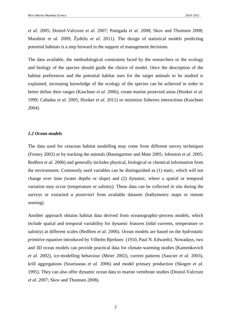
1.2 Ocean models
The data used for cetacean habitat modelling may come from different survey techniques
(Forney 2002) or by tracking the animals (Baumgartner and Mate 2005; Johnston et al. 2005;
Redfern et al. 2006) and generally includes physical, biological or chemical information from
the environment. Commonly used variables can be distinguished as (1) static, which will not
change over time (water depths or slope) and (2) dynamic, where a spatial or temporal
variation may occur (temperature or salinity). These data can be collected in situ during the
surveys or extracted a posteriori from available datasets (bathymetric maps or remote
sensing).
Another approach obtains habitat data derived from oceanographic-process models, which
include spatial and temporal variability for dynamic features (tidal currents, temperature or
salinity) at different scales (Redfern et al. 2006). Ocean models are based on the hydrostatic
primitive equation introduced by Vilhelm Bjerknes (1910, Paul N. Edwards). Nowadays, two
and 3D ocean models can provide practical data for climate-warming studies (Kamenkovich
et al. 2002), ice-modelling behaviour (Meier 2002), current patterns (Saucier et al. 2003),
krill aggregations (Sourisseau et al. 2006) and model primary production (Skogen et al.
1995). They can also offer dynamic ocean data to marine vertebrate studies (Doniol-Valcroze
et al. 2007; Skov and Thomsen 2008).

Mres Marine Mammal Science 2010/ 2011
3
Since marine mammals are not always available to be observed during surveys, satellite
tracking (using animal-borne tags) can indicate where the animals are, how much time they
spend on the selected areas and the what are the conditions they experience below the surface
(Johnston et al. 2005; Biuw et al. 2007; Sveegaard et al. 2011). However, these can come at
an important economic cost. The development of highly complex but realistic 3D ocean
models, can offer the possibility of investigating the vertical environment where the animals
were sighted, without the handicap of handling and tagging. Nevertheless, with this approach,
we are not specifying whether the animal was using the entire water column but a general
idea can be obtained on the motivation underlying the use of that particular area not only on
the surface, but at different depths.
1.3 The Gulf of St. Lawrence
The Gulf of St. Lawrence is located in the eastern shore of Canada on the North-West
Atlantic Ocean (Fig1). It is considered a semi-enclosed sea due to its geography, surrounded
by the Quebec shore on the north, Newfoundland on the East and Nova Scotia throughout the
West and South-West. It opens to the ocean by Cabot Strait (the biggest entrance to the Gulf)
and the Strait of Belle Isle and covers a total area of 236,000 km2 making it the world’s
largest estuary (Dickie and Trites 1983).
Fig. 1: Location of the Gulf of St Lawrence, North-West Atlantic (Canada). The blue rectangle indicates the study area which is described in further detail in section 2.1
Mres Marine Mammal Science 2010/ 2011
4
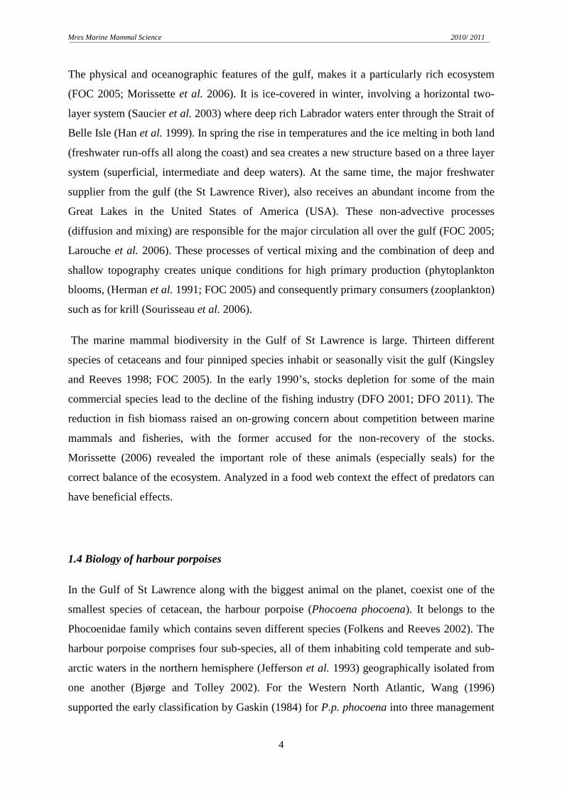
The physical and oceanographic features of the gulf, makes it a particularly rich ecosystem
(FOC 2005; Morissette et al. 2006). It is ice-covered in winter, involving a horizontal two-
layer system (Saucier et al. 2003) where deep rich Labrador waters enter through the Strait of
Belle Isle (Han et al. 1999). In spring the rise in temperatures and the ice melting in both land
(freshwater run-offs all along the coast) and sea creates a new structure based on a three layer
system (superficial, intermediate and deep waters). At the same time, the major freshwater
supplier from the gulf (the St Lawrence River), also receives an abundant income from the
Great Lakes in the United States of America (USA). These non-advective processes
(diffusion and mixing) are responsible for the major circulation all over the gulf (FOC 2005;
Larouche et al. 2006). These processes of vertical mixing and the combination of deep and
shallow topography creates unique conditions for high primary production (phytoplankton
blooms, (Herman et al. 1991; FOC 2005) and consequently primary consumers (zooplankton)
such as for krill (Sourisseau et al. 2006).
The marine mammal biodiversity in the Gulf of St Lawrence is large. Thirteen different
species of cetaceans and four pinniped species inhabit or seasonally visit the gulf (Kingsley
and Reeves 1998; FOC 2005). In the early 1990’s, stocks depletion for some of the main
commercial species lead to the decline of the fishing industry (DFO 2001; DFO 2011). The
reduction in fish biomass raised an on-growing concern about competition between marine
mammals and fisheries, with the former accused for the non-recovery of the stocks.
Morissette (2006) revealed the important role of these animals (especially seals) for the
correct balance of the ecosystem. Analyzed in a food web context the effect of predators can
have beneficial effects.
1.4 Biology of harbour porpoises
In the Gulf of St Lawrence along with the biggest animal on the planet, coexist one of the
smallest species of cetacean, the harbour porpoise (Phocoena phocoena). It belongs to the
Phocoenidae family which contains seven different species (Folkens and Reeves 2002). The
harbour porpoise comprises four sub-species, all of them inhabiting cold temperate and sub-
arctic waters in the northern hemisphere (Jefferson et al. 1993) geographically isolated from
one another (Bjørge and Tolley 2002). For the Western North Atlantic, Wang (1996)
supported the early classification by Gaskin (1984) for P.p. phocoena into three management

Mres Marine Mammal Science 2010/ 2011
5
units: (1) Gulf of Maine-Bay of Fundy, (2) Gulf of St Lawrence (with an estimated northern
population of 21,000 individuals, Kingsley et al. 1998) and (3) Newfoundland.
Reaching between 160-170cm in length and an average of 70kg harbour porpoises are small
stocky animals without a pronounced beak (Read 1999). It is characterized by a dark-grey
dorsal body and diminishing light pattern towards white to the ventral side. They have a
small and falcate dorsal fin which is the most common feature of a sighting (Fig 2). Their life
span is over 20 years, reaching sexual maturity between 3-5 years old (Lockyer 1995).
Mating occurs shortly after giving birth (between May and June) and pregnancy is around 11
months. Lactation follows for 8-12 months post-partum, meaning that females are capable of
being pregnant while still feeding their calves (Gaskin 1984; Lockyer 1995; Read 1999).
Small groups of three individuals might be formed by a female with the older and a new calf
(Read 1999). Group sizes are normally small (1-8) but larger aggregations have been
recorded occasionally probably for migrating and feeding (Hoek 1992; Jefferson et al. 1993;
Van Waerebeek et al. 2002).
The diet of harbour porpoises varies on a regional and seasonal scale (Jefferson et al. 1993)
and is dominated by gadoids, clupeids and squid in the Western North Atlantic (Smith and
Gaskin 1974; Recchia and Read 1989). In the Gulf of St Lawrence important species such as
cod (Gadus morhua) or hake (Merlucidae) represents a minor percentage of harbour porpoise
intakes. Instead, small schooling fish such as capelin (Mallotus villosus) and herring (Clupea
harengus) are the most important prey items making up to 80% of their diet (Fontaine et al.
1994a). Harbour porpoises require food equivalent to approximately 3.5% of their body
weight to be consumed daily and this percentage can increase in lactating females (Yasui and
Gaskin 1986). These fish species satisfy their daily caloric requirements as described for
similar nearby areas such as the Bay of Fundy (Fontaine et al. 1994a). Therefore, harbour
porpoise occurrence is thought to be linked to their prey distribution (Santos and Pierce
Fig. 2: Draw of the external morphology of harbour porpoise. © Maurizio Würtz (http://www.artescienza.org/)

Mres Marine Mammal Science 2010/ 2011
6
2003). Tidal currents, sea bottom depths, temperature and topography are some of the
physical features described as distribution proxies which favours prey concentration,
enhances primary production and thus determine predator distribution (Watts and Gaskin
1985; Lockyer 1995; Weir and O’Brian 2000; Johnston et al. 2005; Johnston and Read 2007;
Skov and Thomsen 2008; Sveegaard 2011).
Due to their energy requirements, harbour porpoise distribution overlap with fisheries. One of
the major threats affecting this species is by-catch and for the late 1980’s Fontaine (1994b)
estimated mortalities close to 2000 porpoises per year in some portions of Gulf of St.
Lawrence. Most of the incidental entanglements of porpoises seemed to occur in groundfish
nets set for Atlantic cod while foraging on capelin and herring (Fontaine et al. 1994a). A
reduction in incidental catches was suspected in the 1990’s after fisheries moratoria due to
fish stock depletion and was confirmed in the Bay of Fundy (Trippel and Shepherd 2004).
The latest estimations for the Gulf of St Lawrence (based on questionnaires to the fisherman
and at-sea observers) indicate a decrease in harbour porpoise by-catch although the authors
recognize imprecise results (Lesage et al. 2004).
1.5 Aims
Harbour porpoise distribution has been related to many different physical features according
to their prey. While in some areas tidal currents seem to be the principal characteristic, in
others underwater topography, temperature or depths are the patterns that better describe their
occurrence. Since diet is slightly different across regions, distribution could be reflected in
the application of different feeding behaviour techniques in order to maximize the energy
income. Harbour porpoises are not socially interacting animals but large aggregations have
been described most likely for migration and feeding purposes. Therefore, the aims of this
study will be:
• Analyse the habitat use of harbour porpoise from the northern Gulf of St.
Lawrence,
• Investigate the relationship between environmental conditions and harbour
porpoise group sizes in the study area.
Mres Marine Mammal Science 2010/ 2011
7
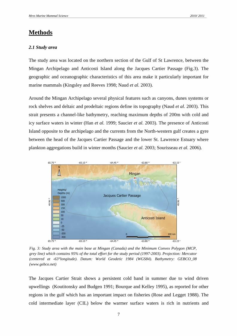
Fig. 3: Study area with the main base at Mingan (Canada) and the Minimum Convex Polygon (MCP, grey line) which contains 95% of the total effort for the study period (1997-2003). Projection: Mercator (centered at -63°longitude). Datum: World Geodetic 1984 (WGS84). Bathymetry: GEBCO_08 (www.gebco.net)
Heights/
Depths (m)
Methods
2.1 Study area
The study area was located on the northern section of the Gulf of St Lawrence, between the
Mingan Archipelago and Anticosti Island along the Jacques Cartier Passage (Fig.3). The
geographic and oceanographic characteristics of this area make it particularly important for
marine mammals (Kingsley and Reeves 1998; Naud et al. 2003).
Around the Mingan Archipelago several physical features such as canyons, dunes systems or
rock shelves and deltaic and prodeltaic regions define its topography (Naud et al. 2003). This
strait presents a channel-like bathymetry, reaching maximum depths of 200m with cold and
icy surface waters in winter (Han et al. 1999; Saucier et al. 2003). The presence of Anticosti
Island opposite to the archipelago and the currents from the North-western gulf creates a gyre
between the head of the Jacques Cartier Passage and the lower St. Lawrence Estuary where
plankton aggregations build in winter months (Saucier et al. 2003; Sourisseau et al. 2006).
The Jacques Cartier Strait shows a persistent cold band in summer due to wind driven
upwellings (Koutitonsky and Budgen 1991; Bourque and Kelley 1995), as reported for other
regions in the gulf which has an important impact on fisheries (Rose and Legget 1988). The
cold intermediate layer (CIL) below the warmer surface waters is rich in nutrients and
Mres Marine Mammal Science 2010/ 2011
8
contributes to the shrimp industry as well as the phytoplankton and nekton communities
(Bourque and Kelley 1995; Naud et al. 2003; Sourisseau et al. 2006). Krill aggregations
remain in this deep layer closely related to bathymetry where they accumulate on most slopes
at the margin of the basin. These aggregations are produced on the eastern side of the strait
where dense Labrador waters from the Strait of Belle Isle pushes organisms along the north
shore of Anticosti Island (Sourisseau et al. 2006). Given the winds and currents occurring in
summer (Han et al. 1999; Saucier et al. 2003), the rich plankton community may attract fish
and thus, the bigger predators.
2.2 Data collection
Data collection was carried out by Mingan Island Cetacean Study (MICS, Longue-Pointe-de-
Mingan, Québec, Canada) as part of their long-term research on baleen whales1. A 7m long
rigid-hulled inflatable boat with outboard engines was employed during the study period
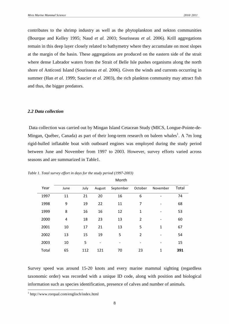
between June and November from 1997 to 2003. However, survey efforts varied across
seasons and are summarized in Table1.
Survey speed was around 15-20 knots and every marine mammal sighting (regardless
taxonomic order) was recorded with a unique ID code, along with position and biological
information such as species identification, presence of calves and number of animals. 1 http://www.rorqual.com/englisch/index.html
Table 1. Total survey effort in days for the study period (1997-2003)
Year
Month
June July August September October November Total
1997 11 21 20 16 6 - 74
1998 9 19 22 11 7 - 68
1999 8 16 16 12 1 - 53
2000 4 18 23 13 2 - 60
2001 10 17 21 13 5 1 67
2002 13 15 19 5 2 - 54
2003 10 5 - - - - 15
Total 65 112 121 70 23 1 391
Mres Marine Mammal Science 2010/ 2011
9
In the early years of this dataset, GPS technology was not available and some sightings were
defined using physical features and subjective measures of distance from shore. Approximate
sighting coordinates were then derived from nautical charts. Areas with numerous small
groups of harbour porpoises were summed over several minutes, resulting in large to very
large group sizes (up to 500 individuals). Initial and ending time and their corresponding
positions were recorded for every track to account for survey effort.
On transect, animal counts were quite precise and recounts of the same animal or group of
animals were considered unlikely. Given the size and behaviour of harbour porpoises, most
of the sightings were within 50m of the boat. In some cases, if animals were spotted further
away, a compass was used to obtain a bearing and an estimated distance was given. Based on
this information a coordinate position was calculated. Overall, it was assumed that harbour
porpoise sightings were contained within 500m from the boat, as their detection decreases
with distance (Palka 1995b).
In the event of a baleen whale sighting, the boat followed the individual to obtain images for
photo-identification purposes. Biopsy samples were also collected or implantable tags
attached for telemetry. However, during these procedures, other marine mammal sightings
were still recorded, but not with the same precision due to the focus on the main activities
mentioned above. This could represent a bias in the data as a result of imprecise counts and
possible re-sampling of harbour porpoise groups while following the baleen whales.
The survey effort was highly dependent on weather conditions, which influenced the area
covered daily and the time spent at sea. In order to avoid potential biases from distant
locations visited only once, a Minimum Convex Polygon (MCP) was generated. The MCP
contained 95% of the total area visited during the entire study period (Appendix A).
Locations falling outside the MCP were not considered for analysis in this study.
Following Doniol-Valcroze et al. (2007; 2008) the environmental data for every sighting was
extracted from the oceanographic model developed by Saucier et al. (2003). This 3D coupled
ice-ocean model is gridded with a horizontal resolution of 5x5km, vertical resolution of 5m
and 5min time-step, offering realistic data for tides, atmospheric, hydrologic and ocean forcing.
These physical variables were derived from pre-defined locations in the study area (model nodes,
App. A). Observed measurements are taken as initial conditions at different depths (to develop
Mres Marine Mammal Science 2010/ 2011
10
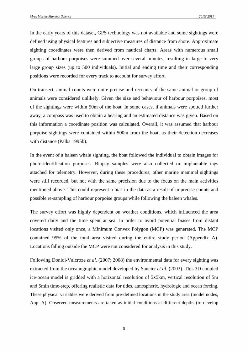
the seasonal model) at specifically designated stations across the Gulf. These stations are located
on the open boundaries, on the Strait of Belle Isle, St. Lawrence Estuary and Cabot Strait (Fig. 4).
Harbour porpoise occurrences were plotted using ArcView 3.1 software and environmental
data was associated by linking the sighting to the nearest 3D node. Temperature (T°), salinity
(S‰), U (East-West), V (North-South) and W (Up/Downwelling) components of water
current (m.s-1) and turbulent kinetic energy (m2s-2) were then calculated from the ocean model
for the specific date-time of the sighting, covering each 5m layer from surface to the
maximum depth of the specific ocean node.
Approximately, 62% of the observation points were lost in the environmental extraction
process. Most of the missing sightings vanished from the dataset for unknown reasons (but
most likely due to the large amount of data) and others were removed because their position
fell outside the grid of the ocean model.
2.3 Generating pseudo-absences
The data obtained during the survey period was solely represented by presences. Different
analysis methods (such as Ecological Niche Factor Analysis, ENFA, or Principal Component
Fig. 4: Open boundaries where oceanographic stations (red circles) retrieve data for the 3D ocean model. From Saucier et al. 2003
Mres Marine Mammal Science 2010/ 2011
11
Analysis, PCA) rely on this type of data, but in order to improve the habitat use analysis
(Brotons et al. 2004; MacLeod et al. 2008), pseudo-absences are created. These false
absences represent locations in the effort area where the target species could have been seen
(a potential suitable area) but assumed they were not at that particular instant in space and
time. Statistically there is no evidence to attribute an absence following this procedure
because of its inherent uncertainty, but it has been proved to be a valuable resource (Doniol-
Valcroze et al. 2007; Žydelis et al. 2011).
For every unique sighting with its correspondent environmental data, a random point was
generated for the same day and time to create an absence location. Pseudo-absences were
distributed randomly within the 95% MCP. Predictive models using presence only data tend
to enlarge the suitable areas for the studied species. Applying this method, explanatory
variables can be better represented in the model and the predictive power of the model highly
improved (Chefaoui and Lobo 2008).
The full dataset containing presences/absences of harbour porpoises with their associated
biological and environmental data produced and personally provided by Thomas Doniol-
Valcroze.
2.4 Analysis
The statistical analysis on this study was conducted with R software (R Core Development
Team 2011) using geepack (Yan and Fine 2004) and car (Fox and Weisberg 2011)
libraries depending on the models and tests to be performed. Maps used to plot results were
generated using Manifold system 8.0 (© CDA International Ltd., 2008). For the present
study, observations with positions not given by a GPS and group sizes over 20 individuals
were dismissed in order to avoid possible biases from the data collection. Given the nature of
the data set an initial standard exploratory analysis was carried out to check for linearity or
patterns in the covariates for both habitat use and group size models.

Mres Marine Mammal Science 2010/ 2011
12
2.4. a) Generalized Linear Models and Generalized Estimating Equations
Generalized linear models (GLMs) are extensions of linear models where the response
variable follows a non-normal distribution (it follows any of the exponential family
distributions instead) and where the mean of the response is a function of the explanatory
variable via a link function (Zuur et al. 2009).
To build a model three steps must be detailed:
(1) The distribution of the response. Let Yi be the response variable, the notation is:
Y i ~ Binomial (ni,p)
(2) The logistic regression model:
logit (ηi)= α+ β1*variable1+…+ βn*variablei
And (3) the link function (logit, ensures model predictions are between 0-1):
����� = log���
1 − ���
Since GLMs allow the response variable to follow a non-normal distribution and non-
constant variance, these models are more flexible and better fitted for ecological data than
standard linear models (Guisan et al. 2002).
However, biological studies frequently result in spatial or temporal correlated data.
Generalized estimating equations (GEEs) are used for nested data where the independence
assumption is violated (Liang and Zeger 1986). As with GLMs, this statistical approach can
be used to model any of the exponential family distributions (Zuur et al. 2009). The steps to
specify a GEE are the same as in a GLM with the addition of a correlation structure.
(1) The systematic part (where i= nested data and s= measure ):
logit (ηis)= α+ β1*variableis+…+ βn*variableis
(2) The random part: Measurements on different groups (or panels) are assumed to be
independent but correlated within the same group. The variance is then related to the

Mres Marine Mammal Science 2010/ 2011
13
mean by a variance function which allows for over-dispersion by estimating a
dispersion parameter:
Var(Yis) = ϕV(pis)
(3) The correlation structure: Needed for the repeated measures and is given in the shape
of a correlation matrix (R (α)). The correlation matrix will describe as much as
possible the correlation between groups. Four different types can be fitted: AR(1),
Unstructured, Independent or Exchangeable (Hardin and Hilbe 2003; Zuur et al.
2009) depending on the data.
2.4. b) Habitat use models
The data supplied by MICS contained sightings of harbour porpoises with associated physical
data and their corresponding pseudo-absence points, with equivalent information. Depending
on the depth of the presence/absence locations, fewer or more environmental data were
available from the different water layers given by the 3D ocean model. A large number of
sites were found to be in shallow areas and thus fewer layers available for analysis. In order
to evaluate and compare the maximum number of observations, only the surface layer was
entered in the computation of the following models.
For the presence/absence distribution a GLM within the binomial family and logit link
function was performed. A model with all the explanatory variables was reduced to the best
fitting model running hypothesis tests performed by Analysis of Deviance (Anova type II
test, using the “car” library) to obtain p-values from a Chi-Square distribution. The covariates
were dropped from the fully saturated model using backwards selection. Once all the
covariates were significant (at a level of significance, α, of 0.05) the explained Deviance (D)
for binary outcomes was calculated to identify the proportion of deviance explained by the
model.
In order to account for possible non-independence in the data, a Binomial-GEE was built as a
fully saturated model and reduced to the best fitting model in a backwards selection process.
The GEE was specified by day as panel with an independent correlation structure. The
underlying reason for the selection of this panel was driven by the physical conditions of the

Mres Marine Mammal Science 2010/ 2011
14
area, influence of winds and currents (Bourque and Kelley 1995; Han et al. 1999), being
more likely the presence of harbour porpoises to be correlated on a daily basis, but
independent across days. The significance of the covariates was determined by Wald chi-
square hypothesis testing set at a 95% confidence level (Rotnitzky and Jewell 1990). This test
performs its analysis adding terms sequentially. Each covariate occupied the last position in
the model to test for its significance and once all the explanatory variables were tested the
one with the highest p-value was dropped from the model. This procedure ran for several
rounds, in which one covariate was removed once the significance of all the variables was
tested. If no existing correlation arises, the model should be the same as the one performed by
the GLM. On the other hand, if a difference between models was detected, the GEE model
was given priority as it would account for the correlation, and thus the biological meaning of
the model would be more accurate.
2.4. c) Group size models
Two Poisson-GLMs with a log link function were performed to investigate the relationship
between the response variables (group size) and the environmental variables. On the first
model all the observed group sizes entered in the analysis whereas in the second model only
the group sizes above the observed mean group size were considered. Due to the highly right-
skewed distribution on the counts, the former was intended to relate group sizes to
environmental conditions while the latest was projected to explore for the likelihood of large
group sizes (up to 20 individuals). To account for possible over-dispersion in the data a full
model with a quasi-poisson link was refitted before the covariates selection. The dispersion
parameter (ϕ) appeared to be higher than one (1.63) and so the models with extra variance
were selected. The fully saturated models were reduced to the best fitting models following
the same method used for the habitat use analysis mentioned above. The D for the Poisson-
GLMs was calculated to quantify the amount of deviance explained by the models in each
case.
GEEs can be considered as an extension of quasi–likelihood models for independent
measurements (Ballinger 2004). Both count GLMs had their own coupled Poisson-GEE
models to be compared so that non-independence in the data could be detected while already
accounting for over-dispersion. The panels and the correlation structures were set to day and

Mres Marine Mammal Science 2010/ 2011
15
independent respectively for both models. Several rounds using Wald chi-squares p-values
(Rotnitzky and Jewell 1990) determined the variables that would be included in the model at
a 0.05 level of significance.
Results
3.1 Survey data
Total distances covered from 1997 to 2003 are summarized in App. B, and on average
8622km (SE ±7522km) were surveyed each year. The number of days spent at sea and the
total number of harbour porpoise sightings recorded is given in Table 1 and App. B
respectively. The dataset offered by MICS included 3751 harbour porpoise sightings and
their linked absences containing seven different environmental variables (Table 2) for the
surface layer given by the 3D ocean model from Saucier et al. (2003).
Table 2. Physical and oceanographic explanatory variables used in the models. The variable Depth refers to the closest ocean model node to the sightings for which the environmental data was derived. The first term in U, V and W component of the water current are described as the positive values. Mean (95% confidence
intervals) and standard deviations (SD) from the sightings, derived from the ocean model nodes are shown.
Explanatory variable Type Units Mean (95% CI) ±SD
Depth Static m 98.05
(96.53-99.58) 43.46
Temperature Dynamic T° 9.12
(9.028-9.215) 2.65
Salinity Dynamic S‰ 28.95
(28.90-29.01) 1.51
U component of water current (East-West)
Dynamic m.s-1 0.04
(0.034- 0.06) 0.36
V component of water current (North-South)
Dynamic m.s-1 -0.06
(-0.07/ -0.05) 0.21
W component of water current (Up-Downwelling)
Dynamic m.s-1 1.98 e-05
(1.628 e-05-2.326 e-05) 9.93 e-05
TKE turbulent kinetic energy Dynamic m2s-2 0.00022
(0.00013-0.00030) 0.0024

Mres Marine Mammal Science 2010/ 2011
16
Along with this information, the GPS position of the sighting, date, time, month, year and
group size were also specified for every observation. However, because of the
aforementioned potential biases in the data collection (non GPS positions and group sizes
over 20 individuals), 637 records were removed leaving a total of 3114 presences (plus their
linked absences), making up a total of 6228 points entered for the analysis.
3.2 Habitat use models
The GLM-GEE based models differed slightly in some covariates. The meaning of these
differences reflects the temporal autocorrelation in the data. The panel used in the GEE
model was day and so model error correlation was permitted on sightings from the same
days. As a result, the GEE model was the one used for predictions for more feasible
biological meaning. The Wald-statistic test retained the factor Year (χ2 =30.717; p-
value<0.001) although two of these levels (2002, 2003) were not significant. The rest of the
coefficients were all significant at the 0.05 level. The estimated correlation parameter (α) was 0
since the correlation structure was chosen as independent.
The goodness-of-fit of the model was assessed by the Deviance (D) for binary data which
offers an equivalent measure of an R2. The D explained by the GLM model was 0.3 (30%).
Since D is based on a likelihood measure, it cannot be applied to the GEE model. As an
alternative, graphical model validation was performed which returned patterns in the errors
Caution is needed when data are treated with a GEE. Depending on the number of panels
used (usually small), estimates may vary using different correlation structures as well as the
significance of the variables. It is normally recommended to have more than 20 clusters
(Prentice 1988; Ballinger 2004). In this analysis, the number of panels was 282 with a
maximum cluster size of 170. The parameter coefficients for the model are summarized in Table 3.
Based on these estimates, there is compelling evidence that presence of harbour porpoise
groups highly increased with upwelling currents, increased with Longitude and Latitude and
slightly increased with depths. In contrast, lower probabilities of porpoise presence are
associated to warmed water masses or northward currents.

Mres Marine Mammal Science 2010/ 2011
17
Although the predicted probabilities of encounter rose in deeper waters, this estimate was
Month dependent (Fig. 5). June appears to be significantly different from the rest of months
in each year. In June, porpoises are more likely to be seen in shallow waters than in deeper
waters, while the opposite is true for the other months.
As temperature and salinity gradients are often linked and determine water masses, a T/S
diagram was created to predict occurrence subject to these two variables (Fig. 6). The model
suggests that the likelihood of harbour porpoise encounters increase in cold and slightly
saline (estuarine) waters. No differences are appreciated between months, indicating that
physical water preferences are not modified along the season and porpoise’s distribution is
related to areas with a considerable input of freshwater. In this model, harbour porpoises
Table 3. Parameter coefficients for the covariates retained in the binomial GEE model for the habitat use analysis. Year and Month estimates differed across the survey period and the minimum and maximum values of the estimates are given. P-values for these covariates (*) are extracted from the hypothesis testing used with the anova function in the geepack library.
Parametric coefficients Estimate Std. error p-value (Wald-statistic)
Intercept
-199.1000
38.3900
<0.001
Longitude 0.6066 0.1520 <0.001
Latitude 4.7560 0.7995 <0.001
Year ((-0.44)-0.6)* - <0.001*
Month ((-1.34)-(-1.84))* - 0.34*
Temperature -0.1409 0.0500 0.005
Salinity 0.0764 0.0361 0.034
V current -0.7228 0.3368 0.032
W current 2598.0000 675.3000 <0.001
Depth 0.1436 0.0333 <0.001
Depth:Month (0.017-0.021)* - <0.001*
Depth:T5 -0.0024 0.0006 <0.001
Depth:S5 -0.0045 0.0010 <0.001

Mres Marine Mammal Science 2010/ 2011
18
Fig. 5: Predicted occurrences by depths across the season for the years entered in the model. Note than June appears to be the month where sighting probability is higher at shallow waters. Annual differences are suspected but were not tested.
appear to be highly related to upwelling currents and no differences are observed across
seasons or years.
Fig. 6: Predicted hydrographic conditions. The model suggests that the sighting probability increases with lower water temperatures and increasing concentrations in the salinity. Maximum probabilities in the flat top area of this graph, with predicted values of 0.99 in extremely low salinity conditions, should not be considered and will be covered in the next section (Discussion)

Mres Marine Mammal Science 2010/ 2011
19
No differences are appreciated taking into account only for the coordinate position (Fig 7).
This graph suggests that the probabilities of sighting are higher in the north-east region of the
study area (close to the Mingan archipelago). The computational power to develop this graph
did not permit the interaction of more variables and this fact may have caused these similar
results.
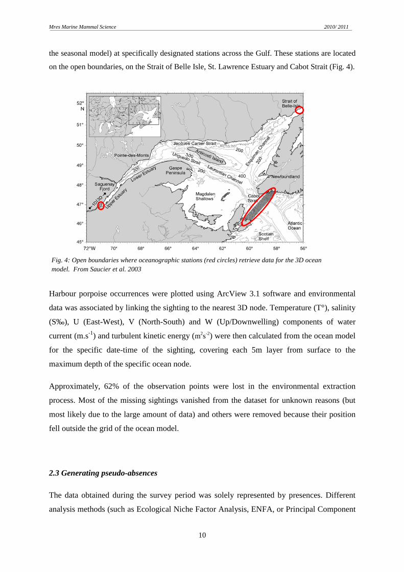
The only variable in the model which reflects any difference in the predicted occurrences
across the season is depth. Prediction maps for two months (June and August) were created to
check for spatial distribution. In June, the GEE model predicted the highest probabilities of
porpoise occurrence in shallow waters, near the coast and over the underwater seamounts
(Fig 8). Predicted sightings in August are localized in the underwater valley north of
Anticosti Island (close to the tail of the Anticosti gyre) and the northern region of the MCP.
The outcome given by the model did not reflect the observed locations for that month,
focusing most of the sightings in the inner, but deeper area of the Jacques Cartier Strait.
Fig. 7: Predicted occurrence based on the geographical position for two months across the season, with mean values for the rest of the variables in the mode. North-east region corresponds to the location of the Mingan archipelago.
Mres Marine Mammal Science 2010/ 2011
20
Fig
. 8
: a
) S
igh
ting
s co
llect
ed
in J
un
e a
cro
ss t
he
su
rve
y p
eri
od
(19
97-
20
03
); b
) P
red
icte
d s
igh
ting
s g
ive
n b
y th
e b
ino
mia
l G
EE
mo
de
l in
Ju
ne
fo
r th
e M
CP
are
a;
c)
Sig
htin
gs
colle
cte
d in
Au
gu
st a
cro
ss t
he
su
rve
y p
er
iod
(1
99
7-2
00
3);
d)
Pre
dic
ted
sig
htin
gs
giv
en
by
the
bin
om
ial G
EE
mo
de
l in
Aug
ust
fo
r th
e M
CP
are
a
a b
c d

Mres Marine Mammal Science 2010/ 2011
21
3.3 Group sizes model
Mean group sizes were similar for the entire study period and were found to be around 2-3
individuals per sighting. The group sizes are highly right skewed being groups bigger than 5
individuals rare. Given the previous analysis of occurrence a coupled GLM-GEE model of
density with Poisson distribution from these observations was modelled. Before the variable
selection process began a quasi-poisson model was fitted to check for over-dispersion in the
data, which resulted in a ϕ value of 1.64. The GLM-GEE pair returned the same variables for
the model, indicating no significant temporal autocorrelation and GLM-Poisson model
preferred. The covariates retained in the model are Latitude and the interaction of year and
depths. The D returned by the model could only explain 2.5% of the variation in the data,
demonstrating a poor fit of the model. Due to this deficient proportion, no more than 3
individuals per group could be predicted while groups of 20 were observed. This
underestimation of the data could be most likely to the scarce large groups observed (groups
5-20 individuals only represented 16.4% of the sightings).
For the last model, only sightings with group sizes over the mean average (more than three
individuals) were modelled. The GLM and the GEE Poisson models differed in the selection
of the most significant variables, representing significant temporal autocorrelation. Under this
circumstance, TKE appeared to be significant in the number of porpoises seen in a group for
the first time. Any of the previous models showed significance for this variable. The GEE
selection process included TKE, V and the interactions formed by depth with Year and
Longitude. Graphical validation revealed weak predictive power with no more than groups of
seven porpoises expected by this model.
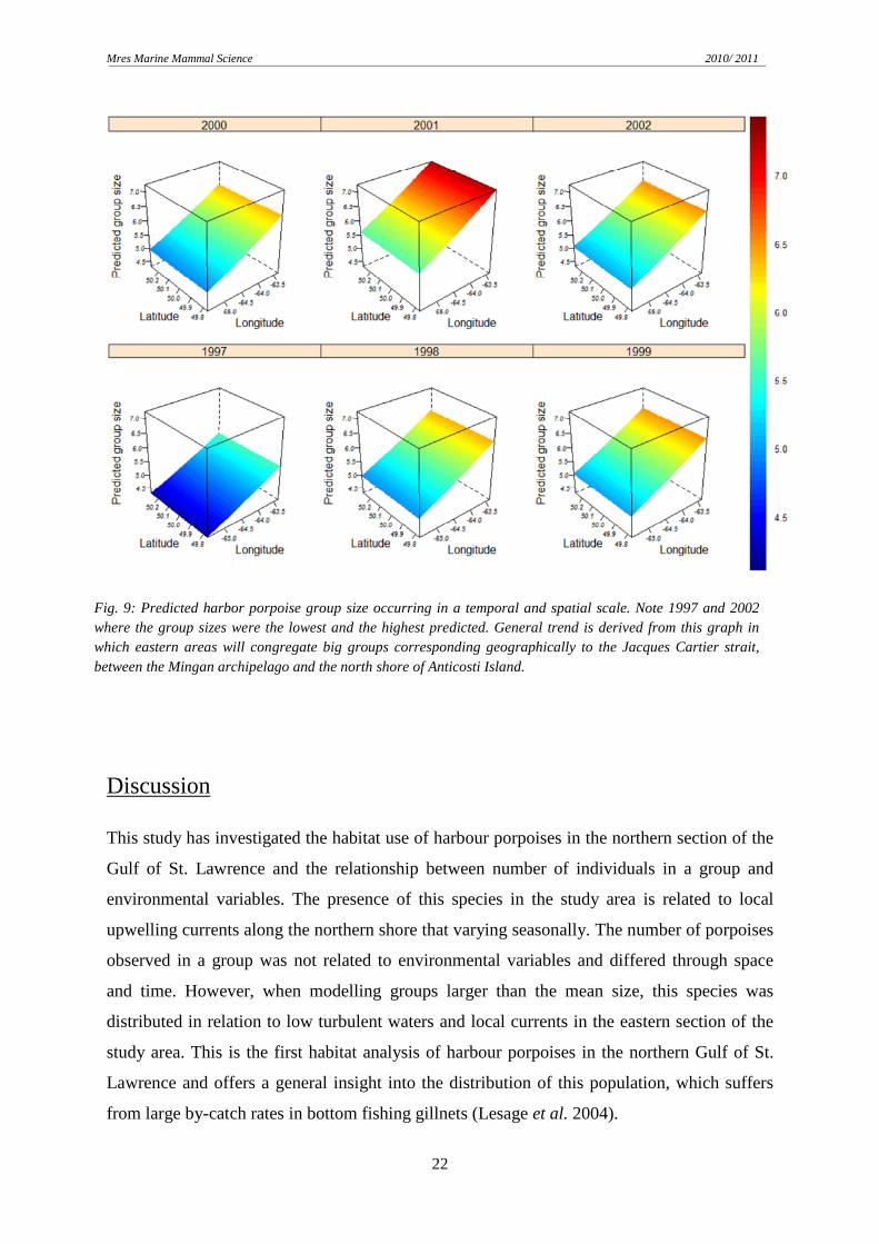
Large groups were predicted to occur in southward currents and low turbulent waters. When
plotting this model for different depths, large interannual variability was discovered. Some
years had bigger groups concentrated in shallow waters while in others, porpoises
congregated in deeper regions. The same phenomenon occurred in a spatial scale (Fig. 9).
Smaller groups were predicted in 1997 while the biggest group size estimation was in 2001
reaching up to 7 individuals. The rest of years considered in the analysis had similar
predictions, but the overall trend was bigger groups occurring in the eastern zone of the study
area, between the Mingan archipelago and the north shore of Anticosti Island (Jacques Cartier
Strait).
Mres Marine Mammal Science 2010/ 2011
22
Discussion
This study has investigated the habitat use of harbour porpoises in the northern section of the
Gulf of St. Lawrence and the relationship between number of individuals in a group and
environmental variables. The presence of this species in the study area is related to local
upwelling currents along the northern shore that varying seasonally. The number of porpoises
observed in a group was not related to environmental variables and differed through space
and time. However, when modelling groups larger than the mean size, this species was
distributed in relation to low turbulent waters and local currents in the eastern section of the
study area. This is the first habitat analysis of harbour porpoises in the northern Gulf of St.
Lawrence and offers a general insight into the distribution of this population, which suffers
from large by-catch rates in bottom fishing gillnets (Lesage et al. 2004).
Fig. 9: Predicted harbor porpoise group size occurring in a temporal and spatial scale. Note 1997 and 2002 where the group sizes were the lowest and the highest predicted. General trend is derived from this graph in which eastern areas will congregate big groups corresponding geographically to the Jacques Cartier strait, between the Mingan archipelago and the north shore of Anticosti Island.
Mres Marine Mammal Science 2010/ 2011
23
The results of the habitat use model suggest a temporal correlation within days motivated by
local currents occurring in the north-eastern sector of the study area. The particular
oceanographic processes in the area, such as the wind-driven upwellings (Bourque and
Kelley 1995), may vary in intensity on a daily basis and thus affect the amount of
zooplankton at the surface. These microorganisms might attract the harbour porpoises’ main
prey to the upper layers, facilitating feeding activity and thus reducing physical effort. Under
favourable upwelling conditions, more sightings will be recorded on the same day. The
higher probabilities observed in the north-east region of the study area can identify two
effects. On the one hand, it offers sheltered areas in the complex topography of the Mingan
Archipelago (Naud et al. 2003) while on the other hand supplies large quantities of prey. The
breeding season of harbour porpoises is short and seasonal (Read 1990), with most of the
births occurring in a nearby area, the Bay of Fundy, in late May-early June (Smith and
Gaskin 1983). The higher predictions of sightings in June would support the hypothesis that
pregnant females search for protected areas to give birth in shallower waters. No information
on the breeding season has been documented for the Gulf of St. Lawrence population but may
become available in future studies. The demanding biological schedule followed by female
porpoises (simultaneous lactation, pregnancy and own survival) would require areas with a
high quantity of available resources to compensate this energy loss in milk production and
gestation. Fortunately, the low energetic requirements of the foetus, allow the mother to
perform both tasks (Read 1999). Within the same context, the porpoise’s main prey in the
study area (capelin and herring) have their spawning events in coastal waters coincident with
the arrival of the porpoises breeding season. Capelin has one large coastal spawn, but
sporadic hatching has been described due to interannual variations in temperature in the west
coast of Newfoundland (DFO 2001). Herring has two spawning stocks in the northern region
of the gulf, in spring and autumn. Tight schools of this pelagic fish start a shoreward
migration in April to spawn along beaches, but can also occur in deeper waters (125m, DFO
2011). This late spring productive peak, could supply the daily energy requirements of
harbour porpoises at a delicate time of the year (Yasui and Gaskin 1986). Following the
completion of capelin and herring first migration, the surviving individuals will undertake the
return journey to deep waters searching for zooplankton. This relocation of prey can be
related to the higher predicted occurrences of harbour porpoises in deeper waters in the
following months. According to previous studies, a large variability exists in an
oceanographic spatial and temporal scale in the Jacques Cartier Strait influencing the annual
primary production and the seasonal distribution of zooplankton (Saucier et al. 2003;
Mres Marine Mammal Science 2010/ 2011
24
Sourisseau et al. 2006). This variability would explain the significance of the variables year
and month added to the model, causing a non-constant monthly and yearly distribution. The
predicted water properties preferred by porpoises did not differ across the season (Fig. 6).
However, it is worth mentioning that the graphical results obtained for this prediction do not
entirely describe the expected trend, and it is most likely an artefact of the predictions code
used for these joined variables. The upper and flat area of the graph retrieves maximum
probabilities in water properties inappropriate from a marine or estuarine environment
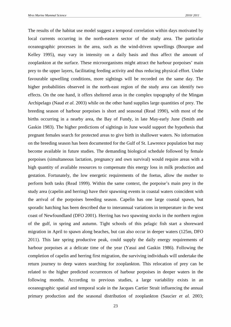
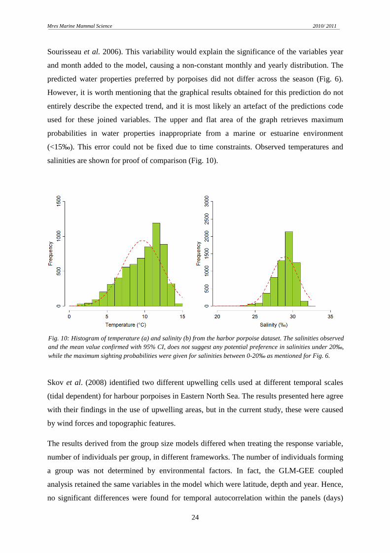
(<15‰). This error could not be fixed due to time constraints. Observed temperatures and
salinities are shown for proof of comparison (Fig. 10).
Skov et al. (2008) identified two different upwelling cells used at different temporal scales
(tidal dependent) for harbour porpoises in Eastern North Sea. The results presented here agree
with their findings in the use of upwelling areas, but in the current study, these were caused
by wind forces and topographic features.
The results derived from the group size models differed when treating the response variable,
number of individuals per group, in different frameworks. The number of individuals forming
a group was not determined by environmental factors. In fact, the GLM-GEE coupled
analysis retained the same variables in the model which were latitude, depth and year. Hence,
no significant differences were found for temporal autocorrelation within the panels (days)
Fig. 10: Histogram of temperature (a) and salinity (b) from the harbor porpoise dataset. The salinities observed and the mean value confirmed with 95% CI, does not suggest any potential preference in salinities under 20‰, while the maximum sighting probabilities were given for salinities between 0-20‰ as mentioned for Fig. 6.
Mres Marine Mammal Science 2010/ 2011
25
but varied across years and location. However, the confidence in this model with a 2.5% of
explained deviance is unconvincing and should not be considered due to its poor quality.
The relationship between large group sizes and environmental variables significantly differed
from the results obtained in the previous Poisson-GLM model. The model for big groups
considered these aggregations as the sets formed by more than three individuals per sighting.
The model presented significant temporal autocorrelation within days and thus the GEE was
used. Bigger groups were predicted to occur in the eastern sector of the study area in southern
currents conditions but low turbulent waters. Hoek (1992) recorded a single event of 800
harbour porpoises in a site close to this study area. The presence of such large aggregations is
not rare (Gaskin 1992; Kingsley and Reeves 1998) in this region and has also been described
in the Bay of Fundy (Read 1990). Yet an improvement was obtained with this model, no
more than seven porpoises per group were predicted, while sightings of up to 20 individuals
were introduced in the analysis. Water depth preferences differed in an interannual mode and
with the exception of 1997 and 1998, the highest predicted group sizes occurred in shallow
waters. These conditions of shallow areas and low turbulence in the eastern sector would
reinforce the theory that there is a calving and nursing area around the Mingan Archipelago
and agrees with the higher observed abundance of harbour porpoise in the Jacques Cartier
Strait (Gaskin 1992; Kingsley and Reeves 1998). Time constraints did not allow investigating
this model in depth, or use the few and hard-computational statistical procedures to validate
the model or explain the importance of the variables could not be inferred.
The analysis carried out in this project employed non-systematic survey methods recording
occurrences of harbour porpoises comprising a wide range of habitat variability (Doniol-
Valcroze 2007). A large number of sightings (7722) were recorded during the study period,
but not the entire dataset could be included in the analysis. The study only focuses on the
harbour porpoise distribution within the MCP, and so the number of sightings missing due to
distant locations did not represent an important loss, but the same is not applied for the extra
lost values. Since the main focus by MICS was not on harbour porpoises, a bias on the
sightability might have been unintentionally introduced. If the emphasis is set to find baleen
whales, the localization of this smaller animal could have involuntary been missed by
inexperienced observers as their sightability decreases with distance (Palka 1995b). In active
search of baleen whales, time spent in some areas may differ from one another and changes
in position due to external factors, such as the weather, could be missed. If no observations

Mres Marine Mammal Science 2010/ 2011
26
were recorded every time the boat changed direction, a bias on the total effort would be
introduced in its computation. Therefore, another approach was considered.
Generating pseudo-absences has proved to be biologically valuable in both land and sea
studies for presence-only data, by allowing some kind of measure of the available space to be
used but assumed it is not at that particular instant in time (Brotons et al. 2004; Doniol-
Valcroze et al. 2007; MacLeod et al. 2008). Creating random points over an area where
porpoises could be seen adds an inherent uncertainty in the data. The probability of an
occurrence at the exact time of a sighting but in a random location over a vast area was not
calculated but can be anticipated to be sufficiently small that would not affect the analysis.
Based on this hypothesis, the data presents locations that would be considered preferred by
the porpoises with other areas of no particular interest.
While focusing in other activities, misdetection and imprecise counts will enter non-realistic
data in the survey. Given the behaviour of this species, incorrect counts in this dataset could
be suspected for large groups due to the lack of an appropriate methodology. A major
concern in counting arises based on how to define a group for these frequently solitary
animals. Several small groups in a big area could be annotated as single events correlated in
time or as a unique observation of numerous individuals in a specific site. Due to equipment
constraints, MICS personnel opted for recording big aggregations as the sum of abundant
smaller groups over a period of time. If this occurrence is very closely related in space and
time, the sum of these smaller groups should be considered as a single event.
Although based on a model and its uncertainty, the environmental data from this ocean model
should be considered adequate (80% goodness-of-fit, Saucier et al. 2003) as positive
economical and ethical aspects are resolved. To study the physical surroundings faced by an
underwater mammal, high technology tags are the only method to directly examine their
habitat. The costs of the tags are avoided here, as well as the capture and handling of the
individual. Nevertheless, an essential limitation is experienced since there is no technique to
recognize whether the individual is using the entire column of water, half of it or just the
surface.
To avoid problems with the non-systematic observations, the GEE model offered the
opportunity to correlate the sightings within days while considering independence across the
survey. This analytical method seemed satisfactory for this data given the diel environmental
variations that occur in the study area created by winds and semi-diurnal tides (Bourque and

Mres Marine Mammal Science 2010/ 2011
27
Kelley 1995; Han et al. 1999). Since the number of strata for each location is determined by
the depth of the sea bottom, a comprehensive analysis of all the layers in the water column
will result in uneven sample sizes. An improved statistical approach could resolve this
problem but time constraints restricted the analysis to the surface layer. In addition,
scheduling did not allow for the performance of different correlation structures and panels for
both the habitat use and group size models. Validation of the model was only given by
graphical summaries where dubious patterns were observed. The non-systematic calculation
of the Quasilikelihood Information Criterion (QIC, Pan 2001) prevented the comparison
between models to account for the better variables to be introduced in the models. This
limitation was undertaken by repeated rounds of Anova, which represented a large amount of
time consumed reducing the full saturated models to the best fitting models. Furthermore,
since the GEEs are based on a quasilikelihood distribution the D explained by the model
could not be obtained and thus the proportion of variation in the data was not identified.
Zheng (2000) developed a formula for marginal models, for instance GEE’s, that he called
Marginal R2 which could be used but time constraints did not allow the computation of this
value. The utilization of this method has increased over the last years (Ballinger 2004;
Panigada et al. 2008; Fieberg et al. 2009) and better models have arisen.
Future work should be focused on the better collection of the biological variables during the
surveys and the systematic tracking of the areas visited per day. The data provided did not
allow for an inference of the effort and this conditioned the generation of the pseudo-
absences. Estimations from better quality data and more biologically descriptive information
(such as behaviour or presence of calves) would improve the analysis. On the early years,
GPS was not available but the development of this technology in the last decade and the
consequent reduction in prices now allows the tracking of all the movements made by the
research vessel. In a statistical context, the large amount of data provided by the ocean model
should be considered in upcoming analysis. The comparison between the significance of
presences in the surface and the adjacent water masses (CIL and deep waters) is encouraged
to be investigated as the zooplankton and prey items are localized at different depths
(Sourisseau et al. 2006). Better techniques to consider for this dataset should include GLMM
and GAMM given the gradual trend in environmental variables (Guisan et al. 2006). Since a
temporal variation was observed over a large scale, individual year models can be attempted
as in Panigada et al. (2008). The methodology and definition used for large groups should be
considered in future seasons in order to better define the causes of this events. The
Mres Marine Mammal Science 2010/ 2011
28
distribution of harbour porpoises in the north shore of Anticosti Island should be considered
in both feeding and social perspectives, since the behaviour and social organisation of
harbour porpoise is poorly understood.
The forthcoming goal to be achieved is to estimate the actual population of harbour porpoises
in this sector of the gulf confirming the calving and nursing area hypothesis in such a rich
feeding ground for marine mammals. The significance of these results can raise the
willingness of a new dedicated survey of abundance (last described in Kingsley and Reeves
1998) in the Northern Gulf of St. Lawrence. The collection of biological parameters (such as
presence of calves) is recommended as the creation of improved habitat models.
Acknowledgements
The development of this project has followed the same life history as a harbour porpoise:
short and intense. Thanks to Richard Sears to kindly reply an e-mail before embarking on the
field. To Christian Ramp to convince me to undertake this long journey, before starting the
new season, Sonja Heinrich to accept supervising it and Clint Blight for the useful maps. To
Thomas Doniol-Valcroze for very valuable comments and kindly helping when everything
meant no-sense and for providing the dataset. To the Canadian Hydrographic Service, and
François Saucier as well as Denis Lefaivre (DFO Canada) for providing the environmental
data, and MICS for collecting data all this years. To Ainhoa Martin Balugo and La Caixa
(Post-graduate scholarships in the UK 2010/2011), for offering me the unique and
unbelievable chance to be part of this. For all the Mres students that shared this experience in
the good and the stressful moments, especially Elisa for making me work harder, Jo for all
the English teaching and Kathleen for all the laughs. For the ones home, supporting me in
every decision I make, and the one that left us too early. Last but not the least, deepest thanks
to Debbie Russell for all the teaching, the guidance, the support and the good vibrations in
every step of this project. You are just awesome!

Mres Marine Mammal Science 2010/ 2011
29
References
Acevedo-Gutiérrez, A. (2002). Habitat use. Encyclopedia of marine mammals B. W. W. F. Perrin, and J. G. M. Thewissen (eds.), Academic Press: 524-528.
Ballinger, G. A. (2004). "Using Generalized Estimating Equations for Longitudinal Data Analysis." Organizational Research Methods 7(2): 127-150.
Baumgartner, M. F. and B. R. Mate (2005). "Summer and fall habitat of North Atlantic right whales (Eubalaena glacialis) inferred from satellite telemetry." Canadian Journal of Fisheries and Aquatic Sciences 62(3): 527-543.
Biuw, M., L. Boehme, C. Guinet, M. Hindell, D. Costa, J.-B. Charrassin, F. Roquet, F. Bailleul, M. Meredith, S. Thorpe, Y. Tremblay, B. McDonald, Y.-H. Park, S. R. Rintoul, N. Bindoff, M. Goebel, D. Crocker, P. Lovell, J. Nicholson, F. Monks and M. A. Fedak (2007). "Variations in behavior and condition of a Southern Ocean top predator in relation to in situ oceanographic conditions." Proceedings of the National Academy of Sciences of the United States of America 104(34): 13705–13710.
Bjerknes, V., T. Hesselberg and O. Devik (1910). Dynamic meteorology and hydrography, Carnegie Institution of Washington.
Bjørge, A. and K. A. Tolley (2002). The harbor porpoise. Encyclopedia of Marine Mammals. B. W. W. F. Perrin, and J. G. M. Thewissen (eds.), Academic Press.
Botsford, L. W., J. C. Castilla and C. H. Peterson (1997). "The Management of Fisheries and Marine Ecosystems." Science 277(5325): 509-515.
Bourque, M. C. and D. E. Kelley (1995). "Evidence of wind‐driyen upwelling in jacques‐cartier strait." Atmosphere-Ocean 33(4): 621-637.
Brotons, L., W. Thuiller, M. B. Araújo and A. H. Hirzel (2004). "Presence-absence versus presence-only modelling methods for predicting bird habitat suitability." Ecography 27(4): 437-448.
Cañadas, A., R. Sagarminaga, R. De Stephanis, E. Urquiola and P. S. Hammond (2005). "Habitat preference modelling as a conservation tool: proposals for marine protected areas for cetaceans in southern Spanish waters." Aquatic Conservation: Marine and Freshwater Ecosystems 15(5): 495-521.
Chefaoui, R. M. and J. M. Lobo (2008). "Assessing the effects of pseudo-absences on predictive distribution model performance." Ecological Modelling 210(4): 478-486.
DFO (2001). Capelin of the Estuary and Gulf of St. Lawrence. DFO Science. Stock Status Report B4-03.
DFO (2011). Assessment of the Quebec North Shore (Division 4S) herring stocks in 2010. Can. Sci. Advis. Sec., Sci. Advis. Rep. 2011/007.
Dickie, L. M. and R. W. Trites (1983). "The Gulf of St. Lawrence." Ecosyst. World 26: 403-425. Doniol-Valcroze, T. (2008). Habitat selection and niche characteristics of rorqual whales in the
Northern Gulf of St. Lawrence (Canada). Department of Natural Resource Sciences. Montreal, McGill University. PhD Thesis: 170.
Doniol-Valcroze, T., D. Berteaux, P. Larouche and R. Sears (2007). "Influence of thermal fronts on habitat selection by four rorqual whale species in the Gulf of St. Lawrence." Marine Ecology Progress Series 335: 207-216.
Evans, P. G. H. and J. A. Raga (2001). Marine mammals: biology and conservation, Kluwer Academic/Plenum Publishers.
Fieberg, J., R. H. Rieger, M. C. Zicus and J. S. Schildcrout (2009). "Regression modelling of correlated data in ecology: subject-specific and population averaged response patterns." Journal of Applied Ecology 46(5): 1018-1025.
FOC (2005). The Gulf of St Lawrence. A unique ecosystem. O. S. Branch, Fisheries and Oceans Canada. Cat. No. FS 104-2/2005.
Folkens, P. A. and R. R. Reeves (2002). Guide to marine mammals of the world, A. A. Knopf, National Audubon Society

Mres Marine Mammal Science 2010/ 2011
30
Fontaine, P.-M., M. O. Hammill, C. Barrette and M. C. Kingsley (1994a). "Summer Diet of the Harbour Porpoise (Phocoena phocoena) in the Estuary and the Northern Gulf of St. Lawrence." Canadian Journal of Fisheries and Aquatic Sciences 51(1): 172-178.
Fontaine, P. M., C. Barrette, M. O. Hammill and M. C. S. Kingsley (1994b). Incidental catches of harbour porpoises (Phocoena phocoena) in the Gulf of St. Lawrence and the St. Lawrence River Estuary, Québec, Canada. Rep. Int. Whaling Comm. Spec. Issue No. 15: 159–163.
Forney, K. (2002). Surveys. Encyclopedia of marine mammals B. W. W. F. Perrin, and J. G. M. Thewissen (eds.), Academic Press: 1203-1205.
Forney, K. A. (2000). "Environmental Models of Cetacean Abundance: Reducing Uncertainty in Population Trends." Conservation Biology 14(5): 1271-1286.
Fox, J. and S. Weisberg (2011). An {R} Companion to Applied Regression, Second Edition. Thousand Oaks CA: Sage. URL: http://socserv.socsci.mcmaster.ca/jfox/Books/Companion.
Gaskin, D. E. (1968). "Distribution of Delphinidae (Cetacea) in relation to sea surface temperatures off Eastern and Southern New Zealand." New Zealand Journal of Marine and Freshwater Research 2(3): 527-534.
Gaskin, D. E. (1984). The harbour porpoise Phocoena phocoena (L.): regional populations, status, and information on direct and indirect catches. Rep Int Whal Commn 34: 569-584.
Gaskin, D. E. (1992). "Status of the harbour porpoise, Phocoena phocoena, in Canada." Can. Field-Nat 106: 36-54.
Guisan, A., T. C. Edwards and T. Hastie (2002). "Generalized linear and generalized additive models in studies of species distributions: setting the scene." Ecological Modelling 157(2-3): 89-100.
Guisan, A., A. Lehmann, S. Ferrier, M. Austin, J. M. C. Overton, R. Aspinall and T. Hastie (2006). "Making better biogeographical predictions of species’ distributions." Journal of Applied Ecology 43(3): 386-392.
Guisan, A. and N. E. Zimmermann (2000). "Predictive habitat distribution models in ecology." Ecological Modelling 135(2-3): 147-186.
Hamazaki, T. (2002). "Spatio-temporal prediction models of cetacean habitats in the mid-western North Atlantic Ocean (from Cape Hatteras, North Carolina, USA to Nova Scotia, Canada)." Marine Mammal Science 18(4): 920-939.
Han, G., J. W. Loder and P. C. Smith (1999). "Seasonal-Mean Hydrography and Circulation in the Gulf of St. Lawrence and on the Eastern Scotian and Southern Newfoundland Shelves." Journal of Physical Oceanography 29(6): 1279-1301.
Hardin, J. W. and J. Hilbe (2003). Generalized estimating equations, Chapman & Hall/CRC. Herman, A. W., D. D. Sameoto, C. Shunnian, M. R. Mitchell, B. Petrie and N. Cochrane (1991).
"Sources of zooplankton on the Nova Scotia shelf and their aggregations within deep-shelf basins." Continental Shelf Research 11(3): 211-238.
Hoek, W. (1992). "AN UNUSUAL AGGREGATION OF HARBOR PORPOISES (PHOCOENA PHOCOENA)." Marine Mammal Science 8(2): 152-155.
Hooker, S. K., A. Cañadas, K. D. Hyrenbach, C. Corrigan, J. J. Polovina and R. R. Reeves (2011). "Making protected area networks effective for marine top predators." Endangered Species Research 13(3): 203-218.
Hooker, S. K., H. Whitehead and S. Gowans (1999). "Marine Protected Area Design and the Spatial and Temporal Distribution of Cetaceans in a Submarine Canyon." Conservation Biology 13(3): 592-602.
Jefferson, T. A., S. Leatherwood and M. A. Webber (1993). FAO Species Identification Guide. Marine mammals of the world. Rome.
Johnston, D. W. and A. J. Read (2007). "Flow-field observations of a tidally driven island wake used by marine mammals in the Bay of Fundy, Canada." Fisheries Oceanography 16(5): 422-435.
Johnston, D. W., A. J. Westgate and A. J. Read (2005). "Effects of fine-scale oceanographic features on the distribution and movements of harbour porpoises Phocoena phocoena in the Bay of Fundy." Marine Ecology Progress Series 295: 279-293.
Kamenkovich, Sokolov and Stone (2002). "An efficient climate model with a 3D ocean and statistical-dynamical atmosphere*." Climate Dynamics 19(7): 585-598.
Kaschner, K. (2004). Modelling and mapping of resource overlap between marine mammals and fisheries on a global scale. Vancouver, University of British Columbia. PhD Thesis: 240.

Mres Marine Mammal Science 2010/ 2011
31
Kaschner, K., R. Watson, A. W. Trites and D. Pauly (2006). "Mapping world-wide distributions of marine mammal species using a relative environmental suitability (RES) model." Marine Ecology Progress series 316: 285:310.
Kingsley, M. and R. R. Reeves (1998). "Aerial surveys of cetaceans in the Gulf of St. Lawrence in 1995 and 1996." Canadian Journal of Zoology 76(8): 1529-1550.
Koutitonsky, V. and G. Budgen (1991). The physical oceanography of the Gulf of St. Lawrence; A review with emphasis on the synoptic variablitiy of the motion. The Gulf of St. Lawrence: Small ocean or big estuary? J. C. Therriault, Can. Spec. Pucl. Fish. Aquat. Sci. 113: 57-90.
Larouche, P., J. M. Boucher and É.Thomassin (2006). Development of a surface feature motion estimation system for the Gulf of St. Lawrence using SST images. Canadian Technical Report of Hydrography and Ocean Sciences 250, Ocean Sciences Branch (Fisheries and Oceans Canada): 27.
Lesage, V., J. Keays, S. Turgeon and S. Hurtubise (2004). Incidental catches of harbour porpoises (Phocoena phocoena) in the gillnet fishery of the Estuary and Gulf of St. Lawrence in 2000−2002. Can. Tech. Rep. Fish. Aquat. Sci.2552. 37 p.
Liang, K.-Y. and S. L. Zeger (1986). "Longitudinal data analysis using generalized linear models." Biometrika 73(1): 13-22.
Lockyer, C. (1995). Aspects of the biology of the harbour porpoise, Phocoena phocoena, from British waters. Developments in Marine Biology. L. W. Arnoldus Schytte Blix and U. Øyvind, Elsevier Science. Volume 4: 443-457.
MacLeod, C., L. Mandleberg, C. Schweder, S. Bannon and G. Pierce (2008). "A comparison of approaches for modelling the occurrence of marine animals." Hydrobiologia 612(1): 21-32.
Marubini, F., A. Gimona, P. Evans, P. Wright and G. Pierce (2009). "Habitat preferences and interannual variability in occurrence of the harbour porpoise Phocoena phocoena off northwest Scotland." Marine Ecology Progress Series 381: 297-310.
Meier (2002). "Regional ocean climate simulations with a 3D ice-ocean model for the Baltic Sea. Part 1: model experiments and results for temperature and salinity." Climate Dynamics 19(3): 237-253.
Morissette, L., M. O. Hammill and C. Savenkoff (2006). "THE TROPHIC ROLE OF MARINE MAMMALS IN THE NORTHERN GULF OF ST. LAWRENCE." Marine Mammal Science 22(1): 74-103.
Morris, D. W. (1987). "Ecological Scale and Habitat Use." Ecology 68(2): 362-369. Naud, M.-J., eacute, B. Long, Br, ecirc, J.-C. thes and R. Sears (2003). "Influences of underwater
bottom topography and geomorphology on minke whale (Balaenoptera acutorostrata) distribution in the Mingan Islands (Canada)." Journal of the Marine Biological Association of the United Kingdom 83(04): 889-896.
Palka, D. (1995b). Abundance estimates of the Gulf of Maine harbour porpoise. Reports of the International Whaling Commission, Special Issue 16, 27-50.
Pan, W. (2001). "Akaike's Information Criterion in Generalized Estimating Equations." Biometrics 57(1): 120-125.
Panigada, S., M. Zanardelli, M. MacKenzie, C. Donovan, F. Mélin and P. S. Hammond (2008). "Modelling habitat preferences for fin whales and striped dolphins in the Pelagos Sanctuary (Western Mediterranean Sea) with physiographic and remote sensing variables." Remote Sensing of Environment 112(8): 3400-3412.
Paul N. Edwards "Before 1955: Numerical models and the prehistory of AGCMs". Atmospheric general circulation modeling: A participatory history. The American Institute of Physics. http://www.aip.org/history/sloan/gcm/prehistory.html.".
Prentice, R. L. (1988). "Correlated Binary Regression with Covariates Specific to Each Binary Observation." Biometrics 44(4): 1033-1048.
R Core Development Team (2011). R: A language and environment for statistical computing. Vienna, Austria, R Foundation for Statistical Computing ISBN 3-900051-07-0, URL http://www.R-project.org.
Read, A. J. (1990). "Reproductive seasonality in harbour porpoises, Phocoena phocoena, from the Bay of Fundy." Canadian Journal of Zoology 68(2): 284-288.
Read, A. J. (1999). Porpoises, Voyageur Press.
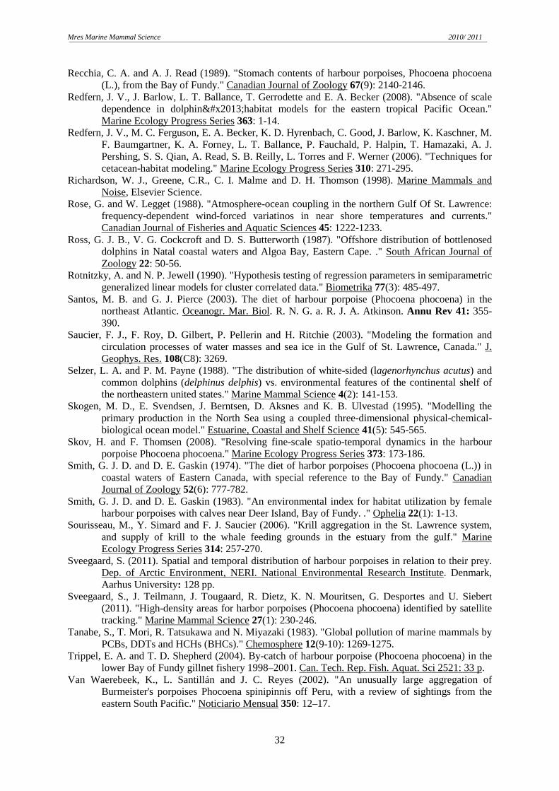
Mres Marine Mammal Science 2010/ 2011
32
Recchia, C. A. and A. J. Read (1989). "Stomach contents of harbour porpoises, Phocoena phocoena (L.), from the Bay of Fundy." Canadian Journal of Zoology 67(9): 2140-2146.
Redfern, J. V., J. Barlow, L. T. Ballance, T. Gerrodette and E. A. Becker (2008). "Absence of scale dependence in dolphin–habitat models for the eastern tropical Pacific Ocean." Marine Ecology Progress Series 363: 1-14.
Redfern, J. V., M. C. Ferguson, E. A. Becker, K. D. Hyrenbach, C. Good, J. Barlow, K. Kaschner, M. F. Baumgartner, K. A. Forney, L. T. Ballance, P. Fauchald, P. Halpin, T. Hamazaki, A. J. Pershing, S. S. Qian, A. Read, S. B. Reilly, L. Torres and F. Werner (2006). "Techniques for cetacean-habitat modeling." Marine Ecology Progress Series 310: 271-295.
Richardson, W. J., Greene, C.R., C. I. Malme and D. H. Thomson (1998). Marine Mammals and Noise, Elsevier Science.
Rose, G. and W. Legget (1988). "Atmosphere-ocean coupling in the northern Gulf Of St. Lawrence: frequency-dependent wind-forced variatinos in near shore temperatures and currents." Canadian Journal of Fisheries and Aquatic Sciences 45: 1222-1233.
Ross, G. J. B., V. G. Cockcroft and D. S. Butterworth (1987). "Offshore distribution of bottlenosed dolphins in Natal coastal waters and Algoa Bay, Eastern Cape. ." South African Journal of Zoology 22: 50-56.
Rotnitzky, A. and N. P. Jewell (1990). "Hypothesis testing of regression parameters in semiparametric generalized linear models for cluster correlated data." Biometrika 77(3): 485-497.
Santos, M. B. and G. J. Pierce (2003). The diet of harbour porpoise (Phocoena phocoena) in the northeast Atlantic. Oceanogr. Mar. Biol. R. N. G. a. R. J. A. Atkinson. Annu Rev 41: 355-390.
Saucier, F. J., F. Roy, D. Gilbert, P. Pellerin and H. Ritchie (2003). "Modeling the formation and circulation processes of water masses and sea ice in the Gulf of St. Lawrence, Canada." J. Geophys. Res. 108(C8): 3269.
Selzer, L. A. and P. M. Payne (1988). "The distribution of white-sided (lagenorhynchus acutus) and common dolphins (delphinus delphis) vs. environmental features of the continental shelf of the northeastern united states." Marine Mammal Science 4(2): 141-153.
Skogen, M. D., E. Svendsen, J. Berntsen, D. Aksnes and K. B. Ulvestad (1995). "Modelling the primary production in the North Sea using a coupled three-dimensional physical-chemical-biological ocean model." Estuarine, Coastal and Shelf Science 41(5): 545-565.
Skov, H. and F. Thomsen (2008). "Resolving fine-scale spatio-temporal dynamics in the harbour porpoise Phocoena phocoena." Marine Ecology Progress Series 373: 173-186.
Smith, G. J. D. and D. E. Gaskin (1974). "The diet of harbor porpoises (Phocoena phocoena (L.)) in coastal waters of Eastern Canada, with special reference to the Bay of Fundy." Canadian Journal of Zoology 52(6): 777-782.
Smith, G. J. D. and D. E. Gaskin (1983). "An environmental index for habitat utilization by female harbour porpoises with calves near Deer Island, Bay of Fundy. ." Ophelia 22(1): 1-13.
Sourisseau, M., Y. Simard and F. J. Saucier (2006). "Krill aggregation in the St. Lawrence system, and supply of krill to the whale feeding grounds in the estuary from the gulf." Marine Ecology Progress Series 314: 257-270.
Sveegaard, S. (2011). Spatial and temporal distribution of harbour porpoises in relation to their prey. Dep. of Arctic Environment, NERI. National Environmental Research Institute. Denmark, Aarhus University: 128 pp.
Sveegaard, S., J. Teilmann, J. Tougaard, R. Dietz, K. N. Mouritsen, G. Desportes and U. Siebert (2011). "High-density areas for harbor porpoises (Phocoena phocoena) identified by satellite tracking." Marine Mammal Science 27(1): 230-246.
Tanabe, S., T. Mori, R. Tatsukawa and N. Miyazaki (1983). "Global pollution of marine mammals by PCBs, DDTs and HCHs (BHCs)." Chemosphere 12(9-10): 1269-1275.
Trippel, E. A. and T. D. Shepherd (2004). By-catch of harbour porpoise (Phocoena phocoena) in the lower Bay of Fundy gillnet fishery 1998–2001. Can. Tech. Rep. Fish. Aquat. Sci 2521: 33 p.
Van Waerebeek, K., L. Santillán and J. C. Reyes (2002). "An unusually large aggregation of Burmeister's porpoises Phocoena spinipinnis off Peru, with a review of sightings from the eastern South Pacific." Noticiario Mensual 350: 12–17.

Mres Marine Mammal Science 2010/ 2011
33
Wang, J. Y., D. E. Gaskin and B. N. White (1996). "Mitochondrial DNA analysis of the harbour porpoise, (Phocoena phocoena), subpopulations in North American waters." Canadian Journal of Fisheries and Aquatic Sciences 53(7): 1632-1645.
Watts, P. and D. E. Gaskin (1985). "Habitat Index Analysis of the Harbor Porpoise (Phocoena phocoena) in the Southern Coastal Bay of Fundy, Canada." Journal of Mammalogy 66(4): 733-744.
Weir, C. and S. O’Brian (2000). Association of the Harbour Porpoise (Phocoena phocoena) with the Western Irish Sea front. Proceedings of the Fourteenth Annual Conference of the European Cetacean Society, Cork, 2-5 April Ireland. pp:61-65
Yan, J. and J. Fine (2004). "Estimating equations for association structures." Statistics in Medicine 23(6): 859-874.
Yasui, W. Y. and D. E. Gaskin (1986). "Energy budget of a small cetacean: The harbour porpoise Phocoena phocoena." L. Ophelia 25: 183–198.
Zheng, B. (2000). "Summarizing the goodness of fit of generalized linear models for longitudinal data." Statistics in Medicine 19(10): 1265-1275.
Zuur, A. F., E. N. Ieno, N. J. Walker, A. A. Saveliev and G. M. Smith (2009). Mixed effects models and extensions in ecology with R, Springer.
Žydelis, R., R. L. Lewison, S. A. Shaffer, J. E. Moore, A. M. Boustany, J. J. Roberts, M. Sims, D. C. Dunn, B. D. Best, Y. Tremblay, M. A. Kappes, P. N. Halpin, D. P. Costa and L. B. Crowder (2011). "Dynamic habitat models: using telemetry data to project fisheries bycatch." Proceedings of the Royal Society B: Biological Sciences.

Mres Marine Mammal Science 2010/ 2011
34
APPENDIX A - METHODS
Fig. A-1: Reconstructed survey effort tracks across the study period from the entire sightings dataset provided by MICS in order to create the MCP containing the 95 % survey effort .From Doniol-Valcroze (2007, 2008)
Fig. A-2: 3D ocean model nodes in the study area where environmental data for sightings and pseudo-absences were retrieved. From Doniol-Valcroze (2008) and Saucier et al (2003)
EFFORT AND OCEAN MODEL NODES

Mres Marine Mammal Science 2010/ 2011
35
Fig. A-3: Harbour porpoise sightings across the study period (1997-2003 provided by MICS
Fig. A-4: Random points (pseudo-absences) created from harbor porpoise sightings within the MCP. Provided by Doniol-Valcroze.
DATA/ RANDOM POINTS

Mres Marine Mammal Science 2010/ 2011
36
APPENDIX B – RESULTS
Table B-1: Total distances from the reconstructed effort tracks in kilometres surveyed per month and year across the study period (1997-2003)
Year
Month
June July August September October November Total
1997 729.14 1889.51 3386.93 2286.13 655.33 - 8947.04
1998 922.43 1776.66 2530.23 1055.15 699.93 - 6984.4
1999 607.19 1328.81 2923.45 1648.32 148.83 - 6656.6
2000 447.61 3262.54 4532.83 1604.57 176.8 - 10024.35
2001 911.61 2020.81 2915 1761.66 282.26 158.52 8049.86
2002 1316.14 3022.38 3768.36 843.85 197.26 - 9147.99
2003 1009.9 911.2 - - - - 1921.1
Total 5944.02 14211.91 20056.8 9199.68 2160.41 158.52 51731.34
Table B-2. Total number of harbour porpoise sightings per month and year across the survey period (1997-2003)
Year
Month
June July August September October November Total
1997 13 52 415 208 146 - 834
1998 4 135 309 39 29 - 516
1999 22 266 470 203 5 - 966
2000 19 846 1073 339 31 - 2308
2001 47 377 819 504 40 3 1790
2002 46 564 436 170 19 - 1235
2003 45 28 - - - - 73
Total 196 2268 3522 1463 270 3 7722
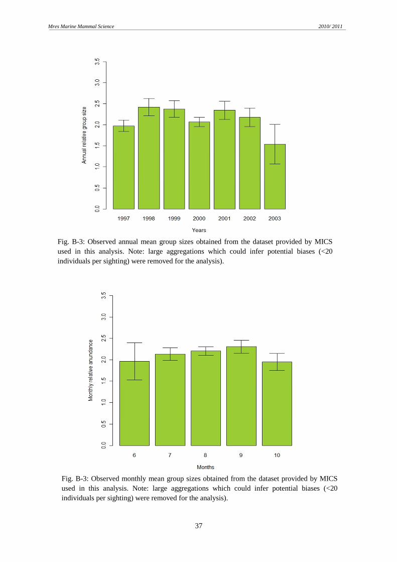
Mres Marine Mammal Science 2010/ 2011
37
Fig. B-3: Observed annual mean group sizes obtained from the dataset provided by MICS used in this analysis. Note: large aggregations which could infer potential biases (<20 individuals per sighting) were removed for the analysis).
Fig. B-3: Observed monthly mean group sizes obtained from the dataset provided by MICS used in this analysis. Note: large aggregations which could infer potential biases (<20 individuals per sighting) were removed for the analysis).