little hankel operators and product bmo - atlanta,...
TRANSCRIPT

OutlineNehari’s Theorem and its Extension
Upper BoundLower Bound & Paraproducts
References
Little Hankel Operators and Product BMO
Michael T. Lacey
Georgia Institute of Technology
March 15, 2005
M.T. Lacey Little Hankels

OutlineNehari’s Theorem and its Extension
Upper BoundLower Bound & Paraproducts
References
Coauthors
Sarah FergusonCUNY Staten Island
Erin TerwillegerU Conn
M.T. Lacey Little Hankels
OutlineNehari’s Theorem and its Extension
Upper BoundLower Bound & Paraproducts
References
1 Nehari’s Theorem and its Extension
2 Upper Bound for Main Theorem
3 Lower Bound & Paraproducts
M.T. Lacey Little Hankels
OutlineNehari’s Theorem and its Extension
Upper BoundLower Bound & Paraproducts
References
CommutatorWeak FactorizationBackground
Hankel and Toeplitz Operators
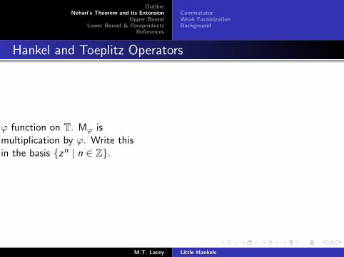
ϕ function on T. Mϕ ismultiplication by ϕ. Write thisin the basis {zn | n ∈ Z}.
We make some restrictions tothe doubly infinite matrix.
M.T. Lacey Little Hankels

OutlineNehari’s Theorem and its Extension
Upper BoundLower Bound & Paraproducts
References
CommutatorWeak FactorizationBackground
Hankel and Toeplitz Operators
ϕ function on T. Mϕ ismultiplication by ϕ. Write thisin the basis {zn | n ∈ Z}.We make some restrictions tothe doubly infinite matrix.
ϕ(0)ϕ(1)ϕ(2)
ϕ(1)
ϕ(2)
M.T. Lacey Little Hankels

OutlineNehari’s Theorem and its Extension
Upper BoundLower Bound & Paraproducts
References
CommutatorWeak FactorizationBackground
Hankel and Toeplitz Operators
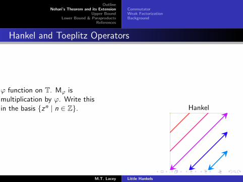
ϕ function on T. Mϕ ismultiplication by ϕ. Write thisin the basis {zn | n ∈ Z}.
We make some restrictions tothe doubly infinite matrix.
Toeplitz
M.T. Lacey Little Hankels
OutlineNehari’s Theorem and its Extension
Upper BoundLower Bound & Paraproducts
References
CommutatorWeak FactorizationBackground
Hankel and Toeplitz Operators
ϕ function on T. Mϕ ismultiplication by ϕ. Write thisin the basis {zn | n ∈ Z}.
We make some restrictions tothe doubly infinite matrix.
Hankel
M.T. Lacey Little Hankels

OutlineNehari’s Theorem and its Extension
Upper BoundLower Bound & Paraproducts
References
CommutatorWeak FactorizationBackground
Nehari’s Theorem (with C. Fefferman H1, BMO duality)
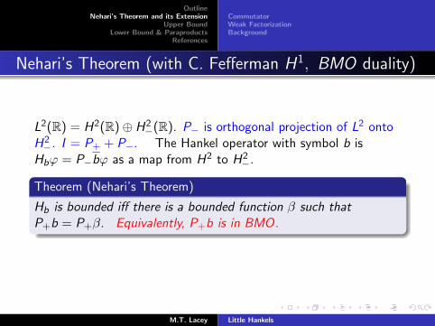
L2(R) = H2(R)⊕ H2−(R). P− is orthogonal projection of L2 onto
H2−. I = P+ + P−.
The Hankel operator with symbol b isHbϕ = P−bϕ as a map from H2 to H2
−.
Theorem (Nehari’s Theorem)
Hb is bounded iff there is a bounded function β such thatP+b = P+β.
Equivalently, P+b is in BMO.
Inner/Outer factorization is key to the proof.
M.T. Lacey Little Hankels

OutlineNehari’s Theorem and its Extension
Upper BoundLower Bound & Paraproducts
References
CommutatorWeak FactorizationBackground
Nehari’s Theorem (with C. Fefferman H1, BMO duality)
L2(R) = H2(R)⊕ H2−(R). P− is orthogonal projection of L2 onto
H2−. I = P+ + P−. The Hankel operator with symbol b is
Hbϕ = P−bϕ as a map from H2 to H2−.
Theorem (Nehari’s Theorem)
Hb is bounded iff there is a bounded function β such thatP+b = P+β.
Equivalently, P+b is in BMO.
Inner/Outer factorization is key to the proof.
M.T. Lacey Little Hankels
OutlineNehari’s Theorem and its Extension
Upper BoundLower Bound & Paraproducts
References
CommutatorWeak FactorizationBackground
Nehari’s Theorem (with C. Fefferman H1, BMO duality)
L2(R) = H2(R)⊕ H2−(R). P− is orthogonal projection of L2 onto
H2−. I = P+ + P−. The Hankel operator with symbol b is
Hbϕ = P−bϕ as a map from H2 to H2−.
Theorem (Nehari’s Theorem)
Hb is bounded iff there is a bounded function β such thatP+b = P+β. Equivalently, P+b is in BMO.
Inner/Outer factorization is key to the proof.
M.T. Lacey Little Hankels

OutlineNehari’s Theorem and its Extension
Upper BoundLower Bound & Paraproducts
References
CommutatorWeak FactorizationBackground
BMO
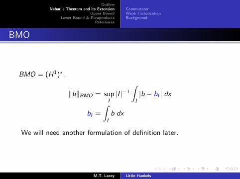
BMO = (H1)∗.
‖b‖BMO = supI|I |−1
∫I|b − bI | dx
bI =
∫Ib dx
We will need another formulation of definition later.
M.T. Lacey Little Hankels

OutlineNehari’s Theorem and its Extension
Upper BoundLower Bound & Paraproducts
References
CommutatorWeak FactorizationBackground
BMO
BMO = (H1)∗.
‖b‖BMO = supI|I |−1
∫I|b − bI | dx
bI =
∫Ib dx
We will need another formulation of definition later.
M.T. Lacey Little Hankels
OutlineNehari’s Theorem and its Extension
Upper BoundLower Bound & Paraproducts
References
CommutatorWeak FactorizationBackground
BMO
BMO = (H1)∗.
‖b‖BMO = supI|I |−1
∫I|b − bI | dx
bI =
∫Ib dx
We will need another formulation of definition later.
M.T. Lacey Little Hankels
OutlineNehari’s Theorem and its Extension
Upper BoundLower Bound & Paraproducts
References
CommutatorWeak FactorizationBackground
Main Theorem
H2(⊗n1C+) denotes the Hardy space of square integrable functions
analytic in each variable separately. Let P be the naturalprojection of L2(⊗n
1C+) onto H2(⊗n1C+). A Hankel operator with
symbol b is the linear operator from H2(⊗n1C+) to H2(⊗n
1C+)given by Hbϕ = Pbϕ.
Theorem
‖Hb‖ ' ‖P⊕b‖BMO(⊗n1C+)
where the right hand norm is the Chang Fefferman product BMO.
M.T. Lacey Little Hankels
OutlineNehari’s Theorem and its Extension
Upper BoundLower Bound & Paraproducts
References
CommutatorWeak FactorizationBackground
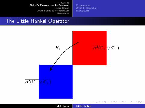
The Little Hankel Operator
H2(C+ ⊗ C+)
H2(C+ ⊗ C+)Hb
M.T. Lacey Little Hankels

OutlineNehari’s Theorem and its Extension
Upper BoundLower Bound & Paraproducts
References
CommutatorWeak FactorizationBackground
Commutator
Define an operator from L2(Rn) to itself by
Cb := [· · · [ [Mb,H1],H2], · · · ,Hn],
in which Mb is the operator of pointwise multiplication by b, andHj denotes the Hilbert transform computed in the jth coordinate.
Corollary
‖Cb‖2 ' ‖b‖BMO(⊗n1R)
This is real BMO.
M.T. Lacey Little Hankels

OutlineNehari’s Theorem and its Extension
Upper BoundLower Bound & Paraproducts
References
CommutatorWeak FactorizationBackground
Weak Factorization of H1(⊗n1C+)
Theorem
A second equivalence gives us a weak factorization result, namely
H1(⊗n1C+) = H2(⊗n
1C+)⊗H2(⊗n1C+)
where the right hand side is the projective tensor product of H2.
‖h‖H2(⊗n1C+)b⊗H2(⊗n
1C+) = inf{∑
j
‖fj‖H2‖gj‖H2 | h =∑
j
fjgj
}
M.T. Lacey Little Hankels
OutlineNehari’s Theorem and its Extension
Upper BoundLower Bound & Paraproducts
References
CommutatorWeak FactorizationBackground
Essential Elements of the Proof
A ‘parameter’ is a free dilation in a coordinate.
The main inequality is ‖Hb‖ & ‖b‖BMO(⊗n1C+). The proof is
inductive on parameters:
The central enemy is the subtle way in which BMO(⊗n1C+) is
built up out of lower parameter BMOs. A new Journe’sLemma is needed to treat this aspect.
A non trivial (but not too dangerous) enemy concerns thedegenerate paraproducts that arise in higher parametersituations.
M.T. Lacey Little Hankels

OutlineNehari’s Theorem and its Extension
Upper BoundLower Bound & Paraproducts
References
CommutatorWeak FactorizationBackground
Background and Notation
L2(R) = H2(C+)⊕ H2(C+), with orthogonal projections P±.
This is extended to L2(⊗n1R) by taking products, thus P±
j is the
one dimensional projection P± applied in the jth coordinate.
P⊕ =n∏
j=1
P+j
Hp(⊗n1C+) is the Hardy space of functions F : ⊗n
j=1C+ −→ C+
that is analytic in each variable separately, and
‖F‖pHp(⊗n
1C+) = lim‖y‖↓0
∫Rn
|F (x + iy)|p dy .
M.T. Lacey Little Hankels

OutlineNehari’s Theorem and its Extension
Upper BoundLower Bound & Paraproducts
References
CommutatorWeak FactorizationBackground
Background and Notation
L2(R) = H2(C+)⊕ H2(C+), with orthogonal projections P±.This is extended to L2(⊗n
1R) by taking products, thus P±j is the
one dimensional projection P± applied in the jth coordinate.
P⊕ =n∏
j=1
P+j
Hp(⊗n1C+) is the Hardy space of functions F : ⊗n
j=1C+ −→ C+
that is analytic in each variable separately, and
‖F‖pHp(⊗n
1C+) = lim‖y‖↓0
∫Rn
|F (x + iy)|p dy .
M.T. Lacey Little Hankels
OutlineNehari’s Theorem and its Extension
Upper BoundLower Bound & Paraproducts
References
CommutatorWeak FactorizationBackground
The Y. Meyer Wavelet
w is a particular Schwartz function w(ξ) supported on [2/3, 8/3].The compact frequency implies that w is rapidly decreasing, andsupported on the whole real line.‘‘Schwarz tails.” Their control dictates most of the technicalitiesof the proof.
M.T. Lacey Little Hankels

OutlineNehari’s Theorem and its Extension
Upper BoundLower Bound & Paraproducts
References
CommutatorWeak FactorizationBackground
The Y. Meyer Wavelet, Cont’d
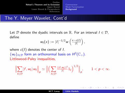
Let D denote the dyadic intervals on R. For an interval I ∈ D,define
wI (x) := |I |−1/2w(
x−c(I )|I |
),
where c(I ) denotes the center of I .
{wI}I∈D form an orthonormal basis on H2(C+).Littlewood-Paley inequalities,∥∥∥∑
I∈D〈f ,wI 〉wI
∥∥∥p'
∥∥∥( ∑I∈D
|〈f ,wI 〉|2|I | 1I
)1/2∥∥∥p, 1 < p <∞.
M.T. Lacey Little Hankels

OutlineNehari’s Theorem and its Extension
Upper BoundLower Bound & Paraproducts
References
CommutatorWeak FactorizationBackground
The Y. Meyer Wavelet, Cont’d
Let D denote the dyadic intervals on R. For an interval I ∈ D,define
wI (x) := |I |−1/2w(
x−c(I )|I |
),
where c(I ) denotes the center of I .{wI}I∈D form an orthonormal basis on H2(C+).
Littlewood-Paley inequalities,∥∥∥∑I∈D
〈f ,wI 〉wI
∥∥∥p'
∥∥∥( ∑I∈D
|〈f ,wI 〉|2|I | 1I
)1/2∥∥∥p, 1 < p <∞.
M.T. Lacey Little Hankels
OutlineNehari’s Theorem and its Extension
Upper BoundLower Bound & Paraproducts
References
CommutatorWeak FactorizationBackground
The Y. Meyer Wavelet, Cont’d
Let D denote the dyadic intervals on R. For an interval I ∈ D,define
wI (x) := |I |−1/2w(
x−c(I )|I |
),
where c(I ) denotes the center of I .{wI}I∈D form an orthonormal basis on H2(C+).Littlewood-Paley inequalities,∥∥∥∑
I∈D〈f ,wI 〉wI
∥∥∥p'
∥∥∥( ∑I∈D
|〈f ,wI 〉|2|I | 1I
)1/2∥∥∥p, 1 < p <∞.
M.T. Lacey Little Hankels

OutlineNehari’s Theorem and its Extension
Upper BoundLower Bound & Paraproducts
References
CommutatorWeak FactorizationBackground
BMO(⊗n1C+) and the Carleson Measure Condition
Let R = ⊗nj=1D be the dyadic rectangles. For a rectangle
R = ⊗nj=1Rj ∈ R, define
vR(x) :=n∏
j=1
wRj(xj).
We say f ∈ BMO(⊗n1C+) iff
supU
[|U|−1
∑R⊂U
|〈f , vR〉|2]1/2
<∞
where U is an open set in Rn of finite measure.
M.T. Lacey Little Hankels

OutlineNehari’s Theorem and its Extension
Upper BoundLower Bound & Paraproducts
References
CommutatorWeak FactorizationBackground
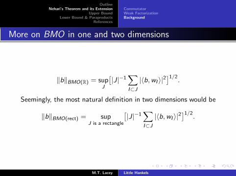
More on BMO in one and two dimensions
‖b‖BMO(R) = supJ
[|J|−1
∑I⊂J
|〈b,wI 〉|2]1/2
.
M.T. Lacey Little Hankels
OutlineNehari’s Theorem and its Extension
Upper BoundLower Bound & Paraproducts
References
CommutatorWeak FactorizationBackground
More on BMO in one and two dimensions
‖b‖BMO(R) = supJ
[|J|−1
∑I⊂J
|〈b,wI 〉|2]1/2
.
Seemingly, the most natural definition in two dimensions would be
‖b‖BMO(rect) = supJ is a rectangle
[|J|−1
∑I⊂J
|〈b,wI 〉|2]1/2
.
M.T. Lacey Little Hankels
OutlineNehari’s Theorem and its Extension
Upper BoundLower Bound & Paraproducts
References
CommutatorWeak FactorizationBackground
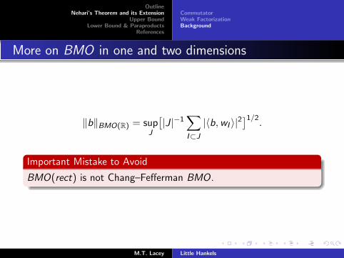
More on BMO in one and two dimensions
‖b‖BMO(R) = supJ
[|J|−1
∑I⊂J
|〈b,wI 〉|2]1/2
.
Important Mistake to Avoid
BMO(rect) is not Chang–Fefferman BMO.
M.T. Lacey Little Hankels

OutlineNehari’s Theorem and its Extension
Upper BoundLower Bound & Paraproducts
References
CommutatorWeak FactorizationBackground
More on BMO in one and two dimensions
‖b‖BMO(R) = supJ
[|J|−1
∑I⊂J
|〈b,wI 〉|2]1/2
.
Important Mistake to Avoid
BMO(rect) is not Chang–Fefferman BMO.
The Journe Lemma is a tool to bound the BMO by rectangularBMO.
M.T. Lacey Little Hankels

OutlineNehari’s Theorem and its Extension
Upper BoundLower Bound & Paraproducts
References
CommutatorWeak FactorizationBackground
S.-Y. Chang R. Fefferman Characterization ofBMO(⊗n
1C+)
Theorem
‖b‖H1(⊗n1C+)∗ ' sup
U
[|U|−1
∑R⊂U
|〈f , vR〉|2]1/2
The “test sets” U are arbitrary measurable subsets Rd of finitemeasure.
M.T. Lacey Little Hankels

OutlineNehari’s Theorem and its Extension
Upper BoundLower Bound & Paraproducts
References
CommutatorWeak FactorizationBackground
Definition of BMO−1(⊗n1C+)
For a collection of rectangles U ⊂ R, set the shadow of U , to be
sh(U) :=⋃
R∈UR.
We say that U has n − 1 parameters
iff there is a coordinate 1 ≤ k ≤ n, and a dyadic interval I , so thatfor all R ∈ U , we have Rk = I
Definition of BMO−1(⊗n1C+)
‖b‖BMO−1(⊗n1C+) = sup
U n − 1 parameters
[|sh(U)|−1
∑R∈U
|〈b, vR〉|2]1/2
M.T. Lacey Little Hankels

OutlineNehari’s Theorem and its Extension
Upper BoundLower Bound & Paraproducts
References
Weak Factorization
Upper Bound on Hankel operator
‖Hb‖ = supf ,g∈H2(⊗n
1C+)‖f ‖2=1,‖g‖2=1
∫(Pbf )g dx
= supf ,g∈H2(⊗n
1C+)‖f ‖2=1,‖g‖2=1
∫P⊕bfg dx .
Since the product of H2 functions is in H1, we see that integralabove admits the upper bound of ‖P⊕b‖BMO(⊗n
1C+). This is theupper half of our Theorem.
M.T. Lacey Little Hankels

OutlineNehari’s Theorem and its Extension
Upper BoundLower Bound & Paraproducts
References
Weak Factorization
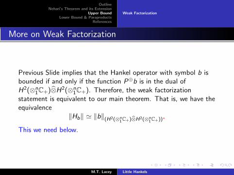
More on Weak Factorization
Previous Slide implies that the Hankel operator with symbol b isbounded if and only if the function P⊕b is in the dual ofH2(⊗n
1C+)⊗H2(⊗n1C+). Therefore, the weak factorization
statement is equivalent to our main theorem. That is, we have theequivalence
‖Hb‖ ' ‖b‖(H2(⊗n1C+)b⊗H2(⊗n
1C+))∗
M.T. Lacey Little Hankels
OutlineNehari’s Theorem and its Extension
Upper BoundLower Bound & Paraproducts
References
Weak Factorization
More on Weak Factorization
Previous Slide implies that the Hankel operator with symbol b isbounded if and only if the function P⊕b is in the dual ofH2(⊗n
1C+)⊗H2(⊗n1C+). Therefore, the weak factorization
statement is equivalent to our main theorem. That is, we have theequivalence
‖Hb‖ ' ‖b‖(H2(⊗n1C+)b⊗H2(⊗n
1C+))∗
This we need below.
M.T. Lacey Little Hankels
OutlineNehari’s Theorem and its Extension
Upper BoundLower Bound & Paraproducts
References
BMO(n − 1) Lower BoundThe BMO Lower BoundApplication of Journe’s LemmaMain EstimateOrthogonality & DiagonalizationThe Positive Sums
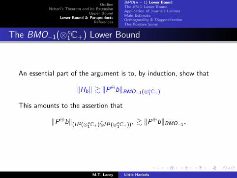
The BMO−1(⊗n1C+) Lower Bound
An essential part of the argument is to, by induction, show that
‖Hb‖ & ‖P⊕b‖BMO−1(⊗n1C+)
This amounts to the assertion that
‖P⊕b‖(H2(⊗n1C+)b⊗H2(⊗n
1C+))∗ & ‖P⊕b‖BMO−1 ,
M.T. Lacey Little Hankels
OutlineNehari’s Theorem and its Extension
Upper BoundLower Bound & Paraproducts
References
BMO(n − 1) Lower BoundThe BMO Lower BoundApplication of Journe’s LemmaMain EstimateOrthogonality & DiagonalizationThe Positive Sums
Take analytic b = b(x1, x2, . . . , xn) = b(x1, x′) of
‖b‖BMO(n−1) = 1.
Take a set U of rectangles n − 1 parameters. Assume that |I | = 1,|sh(U)| = 1, and for all R ∈ U we have R1 = I , and R = I × R ′.Claim: ∥∥∥∑
R∈U〈b, vR〉vR
∥∥∥H2(⊗n
1C+)b⊗H2(⊗n1C+)
. 1.
We have vR(x1, x′) = wI (x1)vR′(x ′), and∑
R∈U〈b, vR〉vR = wI (x1)
∑R∈U
〈b, vR〉vR′(x ′) := wI (x1)ψ′(x ′),
we can utilize factorization results in both x1 and x ′ to concludethe proof.
M.T. Lacey Little Hankels
OutlineNehari’s Theorem and its Extension
Upper BoundLower Bound & Paraproducts
References
BMO(n − 1) Lower BoundThe BMO Lower BoundApplication of Journe’s LemmaMain EstimateOrthogonality & DiagonalizationThe Positive Sums
Take analytic b = b(x1, x2, . . . , xn) = b(x1, x′) of
‖b‖BMO(n−1) = 1.Take a set U of rectangles n − 1 parameters. Assume that |I | = 1,|sh(U)| = 1, and for all R ∈ U we have R1 = I , and R = I × R ′.
Claim: ∥∥∥∑R∈U
〈b, vR〉vR
∥∥∥H2(⊗n
1C+)b⊗H2(⊗n1C+)
. 1.
We have vR(x1, x′) = wI (x1)vR′(x ′), and∑
R∈U〈b, vR〉vR = wI (x1)
∑R∈U
〈b, vR〉vR′(x ′) := wI (x1)ψ′(x ′),
we can utilize factorization results in both x1 and x ′ to concludethe proof.
M.T. Lacey Little Hankels
OutlineNehari’s Theorem and its Extension
Upper BoundLower Bound & Paraproducts
References
BMO(n − 1) Lower BoundThe BMO Lower BoundApplication of Journe’s LemmaMain EstimateOrthogonality & DiagonalizationThe Positive Sums
Take analytic b = b(x1, x2, . . . , xn) = b(x1, x′) of
‖b‖BMO(n−1) = 1.Take a set U of rectangles n − 1 parameters. Assume that |I | = 1,|sh(U)| = 1, and for all R ∈ U we have R1 = I , and R = I × R ′.Claim: ∥∥∥∑
R∈U〈b, vR〉vR
∥∥∥H2(⊗n
1C+)b⊗H2(⊗n1C+)
. 1.
We have vR(x1, x′) = wI (x1)vR′(x ′), and∑
R∈U〈b, vR〉vR = wI (x1)
∑R∈U
〈b, vR〉vR′(x ′) := wI (x1)ψ′(x ′),
we can utilize factorization results in both x1 and x ′ to concludethe proof.
M.T. Lacey Little Hankels

OutlineNehari’s Theorem and its Extension
Upper BoundLower Bound & Paraproducts
References
BMO(n − 1) Lower BoundThe BMO Lower BoundApplication of Journe’s LemmaMain EstimateOrthogonality & DiagonalizationThe Positive Sums
Increasing the Lower Bound
The remainder of the proof is
Concerned with increasing the BMO−1 bound.
Exploits a new form of Journe’s Lemma.
Heavily harmonic analytic, using e.g. orthogonality, LittlewoodPaley, John Nirenberg, etc.
More function theoretic/operator theoretic proofs would bewelcome.
The current proof should provide some hints as what such aproof would look like.
M.T. Lacey Little Hankels
OutlineNehari’s Theorem and its Extension
Upper BoundLower Bound & Paraproducts
References
BMO(n − 1) Lower BoundThe BMO Lower BoundApplication of Journe’s LemmaMain EstimateOrthogonality & DiagonalizationThe Positive Sums
First Steps in Lower Bound
The bound ‖Hb‖ & ‖P⊕b‖BMO(⊗n1C+) can be established under the
assumptions
‖P⊕b‖BMO(⊗n1C+) = 1, ‖P⊕b‖BMO−1(⊗n
1C+) ≤ δ−1,
for a free choice of absolute δ−1 > 0.
Assume that there is collection of rectangles U with |sh(U)| = 1,for which
α =∑R∈U
〈b, vR〉vR
has L2 norm one. Then, we show ‖Hbα‖ & 1.
M.T. Lacey Little Hankels

OutlineNehari’s Theorem and its Extension
Upper BoundLower Bound & Paraproducts
References
BMO(n − 1) Lower BoundThe BMO Lower BoundApplication of Journe’s LemmaMain EstimateOrthogonality & DiagonalizationThe Positive Sums
First Steps in Lower Bound
The bound ‖Hb‖ & ‖P⊕b‖BMO(⊗n1C+) can be established under the
assumptions
‖P⊕b‖BMO(⊗n1C+) = 1, ‖P⊕b‖BMO−1(⊗n
1C+) ≤ δ−1,
for a free choice of absolute δ−1 > 0.Assume that there is collection of rectangles U with |sh(U)| = 1,for which
α =∑R∈U
〈b, vR〉vR
has L2 norm one. Then, we show ‖Hbα‖ & 1.
M.T. Lacey Little Hankels

OutlineNehari’s Theorem and its Extension
Upper BoundLower Bound & Paraproducts
References
BMO(n − 1) Lower BoundThe BMO Lower BoundApplication of Journe’s LemmaMain EstimateOrthogonality & DiagonalizationThe Positive Sums
Application of Journe Lemma
The Function Theoretic Application of Journe Lemma
For any δjourne > 0, We can select V ⊃ sh(U), and a mapemb : U → [1,∞) so that
|V | ≤ 1 + δjourne, emb(R)R ⊂ V ,∥∥∥∑R∈U
emb(R)−2n〈b, vR〉vR
∥∥∥BMO(⊗n
1C+)≤ Kδjourne
δ−1
The power −2n is of no consequence to us. What is important isthe presence of the BMO−1 norm as an upper bound on theBMO(⊗n
1C+) norm.
M.T. Lacey Little Hankels

OutlineNehari’s Theorem and its Extension
Upper BoundLower Bound & Paraproducts
References
BMO(n − 1) Lower BoundThe BMO Lower BoundApplication of Journe’s LemmaMain EstimateOrthogonality & DiagonalizationThe Positive Sums
Geometric Formulation of Journe Lemma
Given a a collection of rectangles U of dyadic rectangles, whoseshadow has finite area, suppose that V ⊃ sh(U), and define
emb(R) := sup{µ ≥ 1 | µR1 × R2 × · · · × Rn ⊂ V }.
For an arbitrary subset U ′ ⊂ U , let
F (I , j ,U ′) :=⋃{I × R ′ | I × R ′ ∈ U ′, 2j−1 ≤ emb(I × R ′) < 2j}.
Notice that these sets are the shadows of collections of rectangleswith n − 1 parameters.
M.T. Lacey Little Hankels

OutlineNehari’s Theorem and its Extension
Upper BoundLower Bound & Paraproducts
References
BMO(n − 1) Lower BoundThe BMO Lower BoundApplication of Journe’s LemmaMain EstimateOrthogonality & DiagonalizationThe Positive Sums
Geometric Formulation of Journe Lemma, Cont’d
Journe Lemma
For all δ, ε > 0, we can select V ⊃ sh(U) with|V | ≤ (1 + δ)|sh(U)|, for which we have the estimate
∞∑j=1
∑I∈D
2−(n+ε)j |F (I , j ,U ′)| . |sh(U ′)|, U ′ ⊂ U .
The implied constants in these estimates depend only ondimensions and the choices of ε, δ.
This estimate is implicit in the work of Pipher.
M.T. Lacey Little Hankels

OutlineNehari’s Theorem and its Extension
Upper BoundLower Bound & Paraproducts
References
BMO(n − 1) Lower BoundThe BMO Lower BoundApplication of Journe’s LemmaMain EstimateOrthogonality & DiagonalizationThe Positive Sums
Images to Keep in Mind
sh(U)
R
V
µR
It is important to expand the rectangle in all directions, in order tocontrol Schwartz tails.
M.T. Lacey Little Hankels

OutlineNehari’s Theorem and its Extension
Upper BoundLower Bound & Paraproducts
References
BMO(n − 1) Lower BoundThe BMO Lower BoundApplication of Journe’s LemmaMain EstimateOrthogonality & DiagonalizationThe Positive Sums
Images to Keep in Mind, Part 2
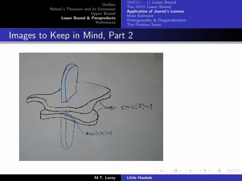
The Carleson Example showsBMO−1(⊗n
1C+) is essentially smaller thanthe BMO(⊗n
1C+) norm. These exampleslive on a “thinly woven fabric” The“embeddedness” quantity pulls out thesethin sheets.
M.T. Lacey Little Hankels
OutlineNehari’s Theorem and its Extension
Upper BoundLower Bound & Paraproducts
References
BMO(n − 1) Lower BoundThe BMO Lower BoundApplication of Journe’s LemmaMain EstimateOrthogonality & DiagonalizationThe Positive Sums
Images to Keep in Mind, Part 2
M.T. Lacey Little Hankels

OutlineNehari’s Theorem and its Extension
Upper BoundLower Bound & Paraproducts
References
BMO(n − 1) Lower BoundThe BMO Lower BoundApplication of Journe’s LemmaMain EstimateOrthogonality & DiagonalizationThe Positive Sums
Elementary Calculations
‖Hαα‖ = ‖P|α|2‖2 & 1.
β :=∑R⊂V
R 6⊂sh(U)
〈b, vR〉vR
‖β‖2 . δ1/2journe, BMO(⊗n
1C+) norm 1, hence small in all Lp.
‖Hβα‖2 . δ1/4journe.
M.T. Lacey Little Hankels

OutlineNehari’s Theorem and its Extension
Upper BoundLower Bound & Paraproducts
References
BMO(n − 1) Lower BoundThe BMO Lower BoundApplication of Journe’s LemmaMain EstimateOrthogonality & DiagonalizationThe Positive Sums
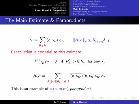
The Main Estimate & Paraproducts
γ :=∑R 6⊂V
〈b, vR〉vR , ‖Hγα‖2 ≤ Kδjourneδ−1
Cancellation is essential to this estimate
Pv ′RvR = 0 if |R ′k | > 8|Rk | for any k.
Hγα =∑
|R′k |≤8|Rk |, all k
〈b, vR′〉〈b, vR〉vR′vR .
This is an example of a (sum of) paraproduct.
M.T. Lacey Little Hankels

OutlineNehari’s Theorem and its Extension
Upper BoundLower Bound & Paraproducts
References
BMO(n − 1) Lower BoundThe BMO Lower BoundApplication of Journe’s LemmaMain EstimateOrthogonality & DiagonalizationThe Positive Sums
The Main Estimate & Paraproducts
γ :=∑R 6⊂V
〈b, vR〉vR , ‖Hγα‖2 ≤ Kδjourneδ−1
Cancellation is essential to this estimate
Pv ′RvR = 0 if |R ′k | > 8|Rk | for any k.
Hγα =∑
|R′k |≤8|Rk |, all k
〈b, vR′〉〈b, vR〉vR′vR .
This is an example of a (sum of) paraproduct.
M.T. Lacey Little Hankels

OutlineNehari’s Theorem and its Extension
Upper BoundLower Bound & Paraproducts
References
BMO(n − 1) Lower BoundThe BMO Lower BoundApplication of Journe’s LemmaMain EstimateOrthogonality & DiagonalizationThe Positive Sums
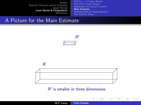
A Picture for the Main Estimate
R
R ′
This choice of R ′ is not allowed.
R ′
Nor is this one.
R ′
R ′ is smaller in one dimension
R ′
Smaller dimension, bigger the gain.
R ′
R ′ is smaller in two dimensions
R ′
R ′ is smaller in three dimensions
M.T. Lacey Little Hankels

OutlineNehari’s Theorem and its Extension
Upper BoundLower Bound & Paraproducts
References
BMO(n − 1) Lower BoundThe BMO Lower BoundApplication of Journe’s LemmaMain EstimateOrthogonality & DiagonalizationThe Positive Sums
A Picture for the Main Estimate
R
R ′
This choice of R ′ is not allowed.
R ′
Nor is this one.
R ′
R ′ is smaller in one dimension
R ′
Smaller dimension, bigger the gain.
R ′
R ′ is smaller in two dimensions
R ′
R ′ is smaller in three dimensions
M.T. Lacey Little Hankels
OutlineNehari’s Theorem and its Extension
Upper BoundLower Bound & Paraproducts
References
BMO(n − 1) Lower BoundThe BMO Lower BoundApplication of Journe’s LemmaMain EstimateOrthogonality & DiagonalizationThe Positive Sums
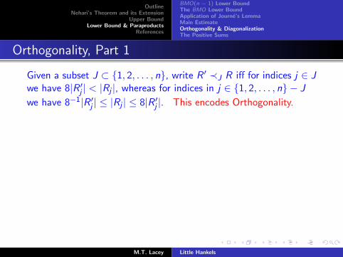
Orthogonality, Part 1
Given a subset J ⊂ {1, 2, . . . , n}, write R ′ ≺J R iff for indices j ∈ Jwe have 8|R ′
j | < |Rj |, whereas for indices in j ∈ {1, 2, . . . , n} − J
we have 8−1|R ′j | ≤ |Rj | ≤ 8|R ′
j |. This encodes Orthogonality.
Set
X (J) := {(R ′,R) ∈ W × U | R ′ ≺J R}
X(J) :=∑
(R′,R)∈X (J)
〈b, vR′〉vR′〈b, vR〉vR .
The remainder of the proof is devoted to the assertion that
‖X(J)‖2 ≤ Kδjourneδ−1, J ⊂ {1, 2, . . . , n}.
M.T. Lacey Little Hankels

OutlineNehari’s Theorem and its Extension
Upper BoundLower Bound & Paraproducts
References
BMO(n − 1) Lower BoundThe BMO Lower BoundApplication of Journe’s LemmaMain EstimateOrthogonality & DiagonalizationThe Positive Sums
Orthogonality, Part 1
Given a subset J ⊂ {1, 2, . . . , n}, write R ′ ≺J R iff for indices j ∈ Jwe have 8|R ′
j | < |Rj |, whereas for indices in j ∈ {1, 2, . . . , n} − J
we have 8−1|R ′j | ≤ |Rj | ≤ 8|R ′
j |. This encodes Orthogonality.Set
X (J) := {(R ′,R) ∈ W × U | R ′ ≺J R}
X(J) :=∑
(R′,R)∈X (J)
〈b, vR′〉vR′〈b, vR〉vR .
The remainder of the proof is devoted to the assertion that
‖X(J)‖2 ≤ Kδjourneδ−1, J ⊂ {1, 2, . . . , n}.
M.T. Lacey Little Hankels
OutlineNehari’s Theorem and its Extension
Upper BoundLower Bound & Paraproducts
References
BMO(n − 1) Lower BoundThe BMO Lower BoundApplication of Journe’s LemmaMain EstimateOrthogonality & DiagonalizationThe Positive Sums
Diagonalization, Part 1
Diagonalization parameters are d1, d2, . . . to gain geometric decayin estimates.
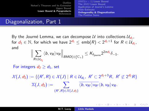
By the Journe Lemma, we can decompose U intocollections Ud1 , for d1 ∈ N, for which we have2d1 ≤ emb(R) < 2d1+1 for R ∈ Ud1 , and∥∥∥ ∑
R∈Ud1
〈b, vR〉vR
∥∥∥BMO(⊗n
1C+)≤ Kδjourne
22nd1δ−1.
For integers d2 ≥ d1, set
X (J, d2) := {(R ′,R) ∈ X (J) | R ∈ Ud1 , R ′ ⊂ 2d2+3R, R ′ 6⊂ 2d2R}
X(J, d2) :=∑
(R′,R)∈X (J,d2)
〈b, vR′〉vR′〈b, vR〉vR .
M.T. Lacey Little Hankels

OutlineNehari’s Theorem and its Extension
Upper BoundLower Bound & Paraproducts
References
BMO(n − 1) Lower BoundThe BMO Lower BoundApplication of Journe’s LemmaMain EstimateOrthogonality & DiagonalizationThe Positive Sums
Diagonalization, Part 1
By the Journe Lemma, we can decompose U into collections Ud1 ,for d1 ∈ N, for which we have 2d1 ≤ emb(R) < 2d1+1 for R ∈ Ud1 ,and ∥∥∥ ∑
R∈Ud1
〈b, vR〉vR
∥∥∥BMO(⊗n
1C+)≤ Kδjourne
22nd1δ−1.
For integers d2 ≥ d1, set
X (J, d2) := {(R ′,R) ∈ X (J) | R ∈ Ud1 , R ′ ⊂ 2d2+3R, R ′ 6⊂ 2d2R}
X(J, d2) :=∑
(R′,R)∈X (J,d2)
〈b, vR′〉vR′〈b, vR〉vR .
M.T. Lacey Little Hankels
OutlineNehari’s Theorem and its Extension
Upper BoundLower Bound & Paraproducts
References
BMO(n − 1) Lower BoundThe BMO Lower BoundApplication of Journe’s LemmaMain EstimateOrthogonality & DiagonalizationThe Positive Sums
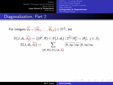
Diagonalization, Part 2
For integers−→d3 = (
−→d31, . . . ,
−→d3 |J|) ∈ N|J|, set
X (J, d2,−→d3) := {(R ′,R) ∈ X (J, d2) | 2
−→d3 j |R ′
j | = |Rj |, j ∈ J},
X(J, d2,−→d3) :=
∑(R′,R)∈X (J,d2,
−→d3)
〈b, vR′〉vR′〈b, vR〉vR
The estimate is:
‖X(J, d2,−→d3)‖2 ≤ Kδjourne
2−d2+‖−→d3‖δ−1.
M.T. Lacey Little Hankels

OutlineNehari’s Theorem and its Extension
Upper BoundLower Bound & Paraproducts
References
BMO(n − 1) Lower BoundThe BMO Lower BoundApplication of Journe’s LemmaMain EstimateOrthogonality & DiagonalizationThe Positive Sums
Diagonalization, Part 2
For integers−→d3 = (
−→d31, . . . ,
−→d3 |J|) ∈ N|J|, set
X (J, d2,−→d3) := {(R ′,R) ∈ X (J, d2) | 2
−→d3 j |R ′
j | = |Rj |, j ∈ J},
X(J, d2,−→d3) :=
∑(R′,R)∈X (J,d2,
−→d3)
〈b, vR′〉vR′〈b, vR〉vR
The estimate is:
‖X(J, d2,−→d3)‖2 ≤ Kδjourne
2−d2+‖−→d3‖δ−1.
M.T. Lacey Little Hankels
OutlineNehari’s Theorem and its Extension
Upper BoundLower Bound & Paraproducts
References
BMO(n − 1) Lower BoundThe BMO Lower BoundApplication of Journe’s LemmaMain EstimateOrthogonality & DiagonalizationThe Positive Sums
Orthogonality Part 2
For R ′ ≺J R and R ′ ≺J R, if for some coordinate j ∈ J we have8|Rj | < |R ′
j |, then vR′vR and veR′veR are orthogonal.
M.T. Lacey Little Hankels

OutlineNehari’s Theorem and its Extension
Upper BoundLower Bound & Paraproducts
References
BMO(n − 1) Lower BoundThe BMO Lower BoundApplication of Journe’s LemmaMain EstimateOrthogonality & DiagonalizationThe Positive Sums
Orthogonality Part 2
For R ′ ≺J R and R ′ ≺J R, if for some coordinate j ∈ J we have8|Rj | < |R ′
j |, then vR′vR and veR′veR are orthogonal.
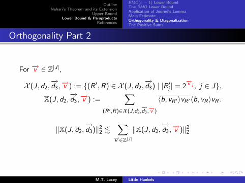
For −→v ∈ Z|J|,
X (J, d2,−→d3,
−→v ) := {(R ′,R) ∈ X (J, d2,−→d3) | |R ′
j | = 2−→v j , j ∈ J},
X(J, d2,−→d3,
−→v ) :=∑
(R′,R)∈X (J,d2,−→d3 ,−→v )
〈b, vR′〉vR′〈b, vR〉vR .
M.T. Lacey Little Hankels
OutlineNehari’s Theorem and its Extension
Upper BoundLower Bound & Paraproducts
References
BMO(n − 1) Lower BoundThe BMO Lower BoundApplication of Journe’s LemmaMain EstimateOrthogonality & DiagonalizationThe Positive Sums
Orthogonality Part 2
For −→v ∈ Z|J|,
X (J, d2,−→d3,
−→v ) := {(R ′,R) ∈ X (J, d2,−→d3) | |R ′
j | = 2−→v j , j ∈ J},
X(J, d2,−→d3,
−→v ) :=∑
(R′,R)∈X (J,d2,−→d3 ,−→v )
〈b, vR′〉vR′〈b, vR〉vR .
‖X(J, d2,−→d3)‖2
2 .∑
−→v ∈Z|J|
‖X(J, d2,−→d3,
−→v )‖22
M.T. Lacey Little Hankels

OutlineNehari’s Theorem and its Extension
Upper BoundLower Bound & Paraproducts
References
BMO(n − 1) Lower BoundThe BMO Lower BoundApplication of Journe’s LemmaMain EstimateOrthogonality & DiagonalizationThe Positive Sums
Orthogonality Part 2
For −→v ∈ Z|J|,
X (J, d2,−→d3,
−→v ) := {(R ′,R) ∈ X (J, d2,−→d3) | |R ′
j | = 2−→v j , j ∈ J},
X(J, d2,−→d3,
−→v ) :=∑
(R′,R)∈X (J,d2,−→d3 ,−→v )
〈b, vR′〉vR′〈b, vR〉vR .
‖X(J, d2,−→d3)‖2
2 .∑
−→v ∈Z|J|
‖X(J, d2,−→d3,
−→v )‖22
Next we replace the product vR′vR above.
M.T. Lacey Little Hankels
OutlineNehari’s Theorem and its Extension
Upper BoundLower Bound & Paraproducts
References
BMO(n − 1) Lower BoundThe BMO Lower BoundApplication of Journe’s LemmaMain EstimateOrthogonality & DiagonalizationThe Positive Sums
The Positive Sums
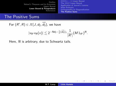
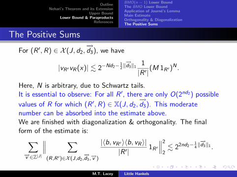
For (R ′,R) ∈ X (J, d2,−→d3), we have
|vR′vR(x)| . 2−Nd2− 12‖−→d3‖1
1
|R ′|(M 1R′)N .
Here, N is arbitrary, due to Schwartz tails.
It is essential to observe: For all R ′, there are only O(2nd2) possible
values of R for which (R ′,R) ∈ X(J, d2,−→d3). This moderate
number can be absorbed into the estimate above.We are finished with diagonalization & orthogonality. The finalform of the estimate is:∑−→v ∈Z|J|
∥∥∥ ∑(R,R′)∈X (J,d2,
−→d3 ,−→v )
|〈b, vR′〉〈b, vR〉||R ′|
1R′
∥∥∥2
2. 22nd2− 1
4‖−→d3‖1 .
M.T. Lacey Little Hankels

OutlineNehari’s Theorem and its Extension
Upper BoundLower Bound & Paraproducts
References
BMO(n − 1) Lower BoundThe BMO Lower BoundApplication of Journe’s LemmaMain EstimateOrthogonality & DiagonalizationThe Positive Sums
The Positive Sums
For (R ′,R) ∈ X (J, d2,−→d3), we have
|vR′vR(x)| . 2−Nd2− 12‖−→d3‖1
1
|R ′|(M 1R′)N .
Here, N is arbitrary, due to Schwartz tails.It is essential to observe: For all R ′, there are only O(2nd2) possible
values of R for which (R ′,R) ∈ X(J, d2,−→d3). This moderate
number can be absorbed into the estimate above.
We are finished with diagonalization & orthogonality. The finalform of the estimate is:∑−→v ∈Z|J|
∥∥∥ ∑(R,R′)∈X (J,d2,
−→d3 ,−→v )
|〈b, vR′〉〈b, vR〉||R ′|
1R′
∥∥∥2
2. 22nd2− 1
4‖−→d3‖1 .
M.T. Lacey Little Hankels
OutlineNehari’s Theorem and its Extension
Upper BoundLower Bound & Paraproducts
References
BMO(n − 1) Lower BoundThe BMO Lower BoundApplication of Journe’s LemmaMain EstimateOrthogonality & DiagonalizationThe Positive Sums
The Positive Sums
For (R ′,R) ∈ X (J, d2,−→d3), we have
|vR′vR(x)| . 2−Nd2− 12‖−→d3‖1
1
|R ′|(M 1R′)N .
Here, N is arbitrary, due to Schwartz tails.It is essential to observe: For all R ′, there are only O(2nd2) possible
values of R for which (R ′,R) ∈ X(J, d2,−→d3). This moderate
number can be absorbed into the estimate above.We are finished with diagonalization & orthogonality. The finalform of the estimate is:∑−→v ∈Z|J|
∥∥∥ ∑(R,R′)∈X (J,d2,
−→d3 ,−→v )
|〈b, vR′〉〈b, vR〉||R ′|
1R′
∥∥∥2
2. 22nd2− 1
4‖−→d3‖1 .
M.T. Lacey Little Hankels

OutlineNehari’s Theorem and its Extension
Upper BoundLower Bound & Paraproducts
References
BMO(n − 1) Lower BoundThe BMO Lower BoundApplication of Journe’s LemmaMain EstimateOrthogonality & DiagonalizationThe Positive Sums
The Essential Difficulty Left to Face
The side lengths of R ′ are for those coordinates in J completelyspecified by −→v ∈ Z|J|. The remaining side lengths of R ′ are thenpermitted to vary. Thus, the ways that two possible choices of
R ′,R ′′ ∈ X (J, d2,−→d3,
−→v ) can intersect are as general as theintersections of two dyadic rectangles of dimension n − |J|.The John Nirenberg, Littlewood Paley Inequalities are the keyingredient to invoke.
M.T. Lacey Little Hankels

OutlineNehari’s Theorem and its Extension
Upper BoundLower Bound & Paraproducts
References
BMO(n − 1) Lower BoundThe BMO Lower BoundApplication of Journe’s LemmaMain EstimateOrthogonality & DiagonalizationThe Positive Sums
The Essential Difficulty Left to Face
Figure: Intersecting 3 dimensional RectanglesM.T. Lacey Little Hankels

OutlineNehari’s Theorem and its Extension
Upper BoundLower Bound & Paraproducts
References
BMO(n − 1) Lower BoundThe BMO Lower BoundApplication of Journe’s LemmaMain EstimateOrthogonality & DiagonalizationThe Positive Sums
John Nirenberg Estimates
John Nirenberg estimates bound high Lp norms in terms of e.g. L1
norms.∥∥∥∥[ ∑
(R′,R)∈X (J,d2,−→d3)
|〈b, vR′〉|2
|R ′|1R′
]1/2∥∥∥∥p
. 24nd2 , 1 < p <∞.
This is immediate from the fact that b is in BMO and that therectangles in X (J, d2,
−→d3,
−→v ) are contained in{M 1sh(U) > c2−nd2}.A similar fact is∥∥∥∥
[ ∑R′∈X (J,d2,
−→d3)
|〈b, vR〉|2
|R|1R′
]1/2∥∥∥∥p
. δ−124nd2 , 1 < p <∞.
M.T. Lacey Little Hankels

OutlineNehari’s Theorem and its Extension
Upper BoundLower Bound & Paraproducts
References
BMO(n − 1) Lower BoundThe BMO Lower BoundApplication of Journe’s LemmaMain EstimateOrthogonality & DiagonalizationThe Positive Sums
John Nirenberg Estimates, Cont’d
What is important here is that the estimate is independent of−→d3,
and is uniform in −→v ∈ Z|J|. Due to the John Nirenberg inequality,this will follow from this estimate.∑
R′⊂V
(R′,R)∈X (J,d2,−→d3)
|〈b, vR〉|2 . 24nd2+‖−→d3‖δ2−1|V |, V ⊂ Rn.
As this estimate is uniform in the choice of V , it provides a boundfor a Carleson measure, to which the John Nirenberg inequalityapplies.
M.T. Lacey Little Hankels

OutlineNehari’s Theorem and its Extension
Upper BoundLower Bound & Paraproducts
References
[1] Sun-Yung A. Chang, Carleson measure on the bi-disc, Ann. of Math. (2)109 (1979), no. 3, 613–620.
[2] Sun-Yung A. Chang and Robert Fefferman, A continuous version of dualityof H1 with BMO on the bidisc, Ann. of Math. (2) 112 (1980), no. 1,179–201.MR 82a:32009
[3] Sarah H. Ferguson and Michael T. Lacey, A characterization of productBMO by commutators, Acta Math. 189 (2002), no. 2, 143–160.1 961 195
[4] Jean-Lin Journe, A covering lemma for product spaces, Proc. Amer. Math.Soc. 96 (1986), no. 4, 593–598.MR 87g:42028
[5] Michael T. Lacey and Erin Terwileger, Little Hankel Operators and ProductBMO.
[6] Jill Pipher, Journe’s covering lemma and its extension to higher dimensions,Duke Math. J. 53 (1986), no. 3, 683–690.MR 88a:42019
M.T. Lacey Little Hankels