Lithosphere

doi: 10.1130/L126.1 published online 23 March 2011;Lithosphere

 Ryan Porter, George Zandt and Nadine McQuarrie for underplated schists and active tectonicsPervasive lower-crustal seismic anisotropy in Southern California: Evidence  

Email alerting servicesarticles cite this article

to receive free e-mail alerts when newwww.gsapubs.org/cgi/alertsclick

Subscribe to subscribe to Lithospherewww.gsapubs.org/subscriptions/click

Permission request to contact GSAhttp://www.geosociety.org/pubs/copyrt.htm#gsaclick

official positions of the Society.citizenship, gender, religion, or political viewpoint. Opinions presented in this publication do not reflectpresentation of diverse opinions and positions by scientists worldwide, regardless of their race, includes a reference to the article's full citation. GSA provides this and other forums for thethe abstracts only of their articles on their own or their organization's Web site providing the posting to further education and science. This file may not be posted to any Web site, but authors may postworks and to make unlimited copies of items in GSA's journals for noncommercial use in classrooms requests to GSA, to use a single figure, a single table, and/or a brief paragraph of text in subsequenttheir employment. Individual scientists are hereby granted permission, without fees or further Copyright not claimed on content prepared wholly by U.S. government employees within scope of

Notes

articles must include the digital object identifier (DOIs) and date of initial publication. priority; they are indexed by PubMed from initial publication. Citations to Advance online prior to final publication). Advance online articles are citable and establish publicationyet appeared in the paper journal (edited, typeset versions may be posted when available Advance online articles have been peer reviewed and accepted for publication but have not

© 2011 Geological Society of America

as doi:10.1130/L126.1Lithosphere, published online on 23 March 2011

LITHOSPHERE

RESEARCH

INTRODUCTION

According to a growing body of geologic and tectonic evidence, the crustal blocks that constitute the crust of southern and central Cali-fornia west of the San Andreas fault are largely the scattered remnants of a once-continuous magmatic arc lithosphere that was delaminated at mid- to lower-crustal levels by Laramide shallow fl at subduction and subsequently underplated by schists derived from the adjacent accretion-ary trench complex (e.g., Saleeby, 2003; Ducea et al., 2009). The end of Laramide fl at subduction was marked by oceanward extensional collapse of the delaminated crust and partial exhumation of the underplated schists (Saleeby, 2003). Post-Laramide tectonic evolution of the region then led to further crustal fragmentation and the transfer of some crustal blocks to the Pacifi c plate, in some cases accompanied by large-magnitude vertical-axis rotation and long-range lateral transport (Nicholson et al., 1994). If this hypothesis is correct, large portions of the crust in southern and west-cen-tral California should be underlain by schists that were overprinted with a fl attening strain during underplating. In this paper, we describe a seismic investigation based on the receiver-function (RF) method to search for and characterize lower-crustal seismic anisotropy that would be expected to delineate such a regional-scale fabric.

Teleseismic receiver functions have been used for roughly the past 30 yr (e.g., Langston, 1979) to better understand crustal structure through the identifi cation of major impedance contrasts and the ratio of P- to

S-wave velocity within layered crust and mantle (e.g., Zandt et al., 1995; Zhu and Kanamori, 2000). More recently, the RF technique has been applied to the identifi cation of anisotropic zones in the crust, which are then used to infer the location and mechanism for previous and current deformation (e.g., Levin and Park, 1997; Savage, 1998; Peng and Hum-phreys, 1997; Sherrington et al., 2004; Ozacar and Zandt, 2004, 2009).

The motivation for this study is the observation of consistent move-out patterns within Southern California indicative of dipping layers or seis-mic anisotropy. Southern California is an ideal location for such a study due to the abundance of geologic and geophysical studies in the region, the availability of numerous long-running (>4 yr) seismic stations with publicly available data, and well-constrained crustal structure and defor-mational history. This well-constrained geologic history helps to address one of the fundamental diffi culties in any seismic analysis, i.e., the lack of temporal information regarding observations. This is especially important in anisotropy analyses, which give no indications as to whether obser-vations refl ect previous deformation or modern tectonics. By interpret-ing our new results in conjunction with previous work in the region, we expect to better constrain the deformational history of the lower crust and improve our understanding of both the regional tectonics and the receiver-function anisotropy technique.

GEOLOGIC AND TECTONIC SETTING

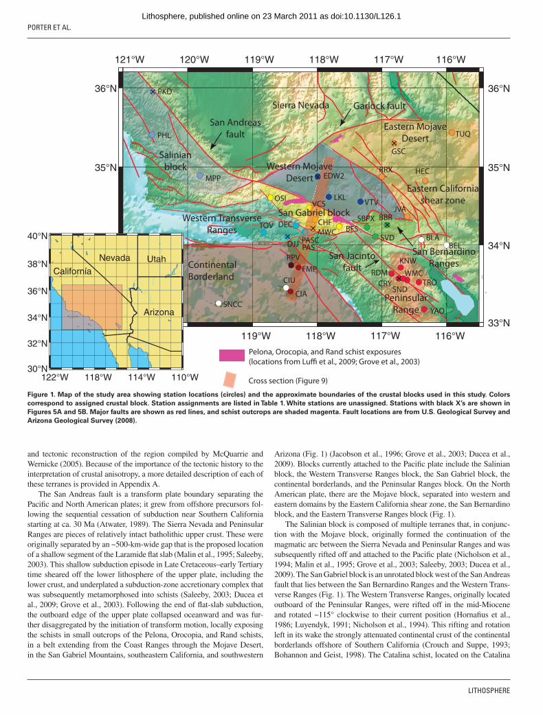
Our study area in Southern California, shown in Figure 1, is composed of two tectonic plates and multiple tectonic terranes with complex geo-logic histories. Here, we will generally follow the terrane terminology

Pervasive lower-crustal seismic anisotropy in Southern California: Evidence for underplated schists and active tectonics

Ryan Porter1*, George Zandt1*, and Nadine McQuarrie2*1DEPARTMENT OF GEOSCIENCES, UNIVERSITY OF ARIZONA, GOULD-SIMPSON BUILDING #77, 1040 E. 4TH STREET, TUCSON, ARIZONA 85721, USA2DEPARTMENT OF GEOSCIENCES, PRINCETON UNIVERSITY, GUYOT HALL, PRINCETON, NEW JERSEY 08544, USA

ABSTRACT

Understanding lower-crustal deformational processes and the related features that can be imaged by seismic waves is an important goal in active tectonics. We demonstrate that teleseismic receiver functions calculated for broadband seismic stations in Southern California reveal a signature of pervasive seismic anisotropy in the lower crust. The large amplitudes and small move-out of the diagnostic converted phases, as well as the broad similarity of data patterns from widely separated stations, support an origin primarily from a basal crustal layer of hexagonal anisotropy with a dipping symmetry axis. We conducted neighborhood algorithm searches for depth and thickness of the anisotropic layer and the trend and plunge of the anisotropy symmetry (slow) axis for 38 stations. The searches produced a wide range of results, but a dominant SW-NE trend of the symmetry axis emerged. When the results are divided into crustal blocks and restored to their pre–36 Ma locations, the regional-scale SW-NE trend becomes more consistent, although a small subset of the results can be attributed to NW-SE shearing related to San Andreas transform motion. We interpret this dominant trend as a fossilized fabric within schists, created from top-to-the-SW sense of shear that existed along the length of coastal California during pretransform, early Tertiary subduction or from shear that occurred during subsequent extrusion. Comparison of receiver-function common conversion point stacks to seismic models from the active Los Angeles Regional Seismic Experiment shows a strong correlation in the location of anisotropic layers with “bright” refl ectors, further affi rming these results.

LITHOSPHERE Data Repository 2011138. doi: 10.1130/L126.1

For permission to copy, contact editing@geosociety.org | © 2011 Geological Society of America

*E-mails: porterrc@email.arizona.edu; gzandt@email.arizona.edu; nmcq@princeton.edu.

as doi:10.1130/L126.1Lithosphere, published online on 23 March 2011

PORTER ET AL.

LITHOSPHERE

and tectonic reconstruction of the region compiled by McQuarrie and Wernicke (2005). Because of the importance of the tectonic history to the interpretation of crustal anisotropy, a more detailed description of each of these terranes is provided in Appendix A.

The San Andreas fault is a transform plate boundary separating the Pacifi c and North American plates; it grew from offshore precursors fol-lowing the sequential cessation of subduction near Southern California starting at ca. 30 Ma (Atwater, 1989). The Sierra Nevada and Peninsular Ranges are pieces of relatively intact batholithic upper crust. These were originally separated by an ~500-km-wide gap that is the proposed location of a shallow segment of the Laramide fl at slab (Malin et al., 1995; Saleeby, 2003). This shallow subduction episode in Late Cretaceous–early Tertiary time sheared off the lower lithosphere of the upper plate, including the lower crust, and underplated a subduction-zone accretionary complex that was subsequently metamorphosed into schists (Saleeby, 2003; Ducea et al., 2009; Grove et al., 2003). Following the end of fl at-slab subduction, the outboard edge of the upper plate collapsed oceanward and was fur-ther disaggregated by the initiation of transform motion, locally exposing the schists in small outcrops of the Pelona, Orocopia, and Rand schists, in a belt extending from the Coast Ranges through the Mojave Desert, in the San Gabriel Mountains, southeastern California, and southwestern

Arizona (Fig. 1) (Jacobson et al., 1996; Grove et al., 2003; Ducea et al., 2009). Blocks currently attached to the Pacifi c plate include the Salinian block, the Western Transverse Ranges block, the San Gabriel block, the continental borderlands, and the Peninsular Ranges block. On the North American plate, there are the Mojave block, separated into western and eastern domains by the Eastern California shear zone, the San Bernardino block, and the Eastern Transverse Ranges block (Fig. 1).

The Salinian block is composed of multiple terranes that, in conjunc-tion with the Mojave block, originally formed the continuation of the magmatic arc between the Sierra Nevada and Peninsular Ranges and was subsequently rifted off and attached to the Pacifi c plate (Nicholson et al., 1994; Malin et al., 1995; Grove et al., 2003; Saleeby, 2003; Ducea et al., 2009). The San Gabriel block is an unrotated block west of the San Andreas fault that lies between the San Bernardino Ranges and the Western Trans-verse Ranges (Fig. 1). The Western Transverse Ranges, originally located outboard of the Peninsular Ranges, were rifted off in the mid-Miocene and rotated ~115° clockwise to their current position (Hornafi us et al., 1986; Luyendyk, 1991; Nicholson et al., 1994). This rifting and rotation left in its wake the strongly attenuated continental crust of the continental borderlands offshore of Southern California (Crouch and Suppe, 1993; Bohannon and Geist, 1998). The Catalina schist, located on the Catalina

-121°33°

34°

-121°33°

34°

Pelona, Orocopia, and Rand schist exposures

(locations from Luffi et al., 2009; Grove et al., 2003)

Cross section (Figure 9)

121°W 120°W 119°W 118°W 117°W 116°W

33°N

34°N

35°N

36°N

35°N

36°N

116°W119°W 118°W 117°W

122°W 118°W 114°W 110°W30°N

32°N

34°N

36°N

38°N

40°N

Eastern California

shear zone

California

Arizona

Nevada UtahContinental

Borderland

Salinian

block

Sierra Nevada

San Andreas

fault

MPP

PHL

PKD

SNCC

Western Mojave Desert

Western Transverse

Ranges

Eastern Mojave

Desert

Garlock fault

TUQ

EDW2

LKLVTV

San Jacinto

fault

CIA

DJJ

FMP

CHFMWC

VCSSan Gabriel blockDECTOV

OSI

RRX

GSC

HEC

San Bernardino

Ranges

Peninsular

Range

BBR

BLA

CRY

JVA

RDM

SBPX

SVD

YAQ

BEL

KNW

SNDTRO

WMCCIU

PASPASC

RPV

BFS

Figure 1. Map of the study area showing station locations (circles) and the approximate boundaries of the crustal blocks used in this study. Colors

correspond to assigned crustal block. Station assignments are listed in Table 1. White stations are unassigned. Stations with black X’s are shown in

Figures 5A and 5B. Major faults are shown as red lines, and schist outcrops are shaded magenta. Fault locations are from U.S. Geological Survey and

Arizona Geological Survey (2008).

as doi:10.1130/L126.1Lithosphere, published online on 23 March 2011

LITHOSPHERE

Pervasive lower-crustal seismic anisotropy in Southern California | RESEARCH

Islands in the offshore borderlands, is another outcrop of subduction-zone accretionary material that was partially subducted beneath the western edge of the Peninsular Ranges Batholith and later exhumed (Grove and Bebout, 1995). The opening of the Gulf of California completed the trans-fer of the Salinian block, Western Transverse Ranges, and the Peninsular Ranges to the Pacifi c plate by ca. 6 Ma (e.g., McQuarrie and Wernicke, 2005). The terranes that remain part of North America are the Mojave, San Bernardino, and the Eastern Transverse Ranges. The Mojave region experienced two stages of Cenozoic deformation: a mid-Tertiary stage of extension associated with core complexes (Glazner et al., 1989; Walker et al., 1990; Martin et al., 1993; Fletcher et al., 1995), and a later stage of right-lateral shear associated with the modern Eastern California shear zone (Dokka and Travis, 1990; Howard and Miller, 1992; McQuarrie and Wernicke, 2005). The San Bernardino block is a relatively small block with a poorly constrained rotational history, located just northwest of the Eastern Transverse Ranges and immediately south of the Mojave block (Stewart and Poole, 1974; Miller, 1981; Luyendyk, 1991). The 38 long-running broadband seismic stations used in this study are located in eight of these terranes (Fig. 1; Table 1).

CRUSTAL SEISMIC ANISOTROPY

Seismic anisotropy is the property of rocks such that the seismic wave speed at a point is dependent on the direction of wave propagation. Here, we follow the defi nition of percent seismic anisotropy as (V

max – V

min) / V

avg,

where V is seismic velocity. Seismic anisotropy in the crust is generally attributed to fractures, rock fabrics, aligned mineral grains, metamor-phism, or magma injection into a shear zone (Babuska and Cara, 1991; Okaya and Christensen, 2002; Okaya and McEvilly, 2003). While aligned fractures play a signifi cant role in upper-crustal anisotropy, once a con-fi ning pressure of 150–300 MPa is achieved, the infl uence of fractures is almost nonexistent (Barruol and Kern, 1996; Pellerin and Christensen, 1998). For lower-crustal rocks, the primary mechanism of anisotropy is believed to be the lattice-preferred orientation (LPO) of mineral grains (also referred to as crystallographic preferred orientation [CPO]; Babuska and Cara, 1991; Levin and Park, 1998). While magma injection into shear zones can create a fabric (Kohlstedt and Holtzman, 2009) capable of pro-ducing seismic anisotropy, this process has been explored much less than LPO anisotropy.

Although most crustal minerals exhibit some form of seismic anisot-ropy, magmatic rocks commonly do not have strong anisotropic signa-tures, due to a lack of aligned mineral grains. Measurable anisotropy is generally found in metamorphic rocks such as schists and gneisses, which are capable of producing seismic anisotropy values as large as 20%, due to the alignment of minerals such as micas (Babuska and Cara, 1991). There are several different forms of seismic anisotropy, which are defi ned by the number of unique values necessary to describe their elas-tic properties (Babuska and Cara, 1991). For this work, we assume hex-agonal anisotropy, also referred to as transverse isotropy. This is the sim-plest form of seismic anisotropy and can be described with one unique velocity axis. The advantage of assuming this form of anisotropy is that it can be parameterized more easily than other forms, requiring a stiff-ness tensor with only fi ve independent variables (compared to two for an isotropic medium). These variables are related to Vp-fast, Vp-slow, Vs-fast, Vs-slow, and Vp-45°, which defi nes the velocity gradient between Vp-fast and Vp-slow (see Appendix B) (Okaya and Christensen, 2002; Babuska and Cara, 1991). Following hexagonal anisotropy, the next sim-plest form of anisotropy is orthorhombic, which requires nine unique variables to describe the elastic tensor. This high number of unique vari-ables makes an inversion for these parameters from receiver-function

data untenable given current seismic analysis techniques and data. For-tunately, several studies have suggested that hexagonal anisotropy is suf-fi cient to describe the average aggregate properties of regionally signifi -cant zones of crustal anisotropy (e.g., Levin and Park, 1997; Godfrey et al., 2000). A similar argument is used to justify using hexagonal anisot-ropy to describe the anisotropic effect of an aggregate of orthorhombic olivine crystals in the upper mantle.

Hexagonal anisotropy can be divided into two different categories: fast unique axis and slow unique axis (or pumpkin and melon, respec-tively, in the terminology of Levin and Park, 1997) (Fig. 2). Fast-axis anisotropy is seen in mantle rocks (e.g., olivine) and is used for SKS wave-splitting analysis, which generally assumes a horizontal orienta-tion of the fast axis. Results from SKS measurements are commonly dis-played in maps of fast-axis orientations. In the Southern California crust, we expect to fi nd regionally pervasive crustal schist packages with abun-dant micas defi ning a foliation (Fig. 2). Micas within the schist would dominate the anisotropic signature of the rock and therefore are believed to be the primary source of observed anisotropy (Weiss et al., 1999). Typical micas are monoclinic but have seismic anisotropy that deviates only slightly from strong slow-axis hexagonal anisotropy (Alexandrov and Ryzhova [1961] in Babuska and Cara, 1991; Vaughan and Guggen-heim, 1986); hence slow-axis hexagonal anisotropy is often assumed for crustal anisotropy studies (Weiss et al., 1999). We will follow this convention in this study and will display results in maps of slow-axis orientations. Unlike the upper-mantle case, where the horizontal fast-axis orientation can only resolve the shear axis and not the direction of deformation, the uniquely dipping, slow-axis trend potentially can be used to determine the sense of shear within a subhorizontal shear zone. If shearing within the zone produces a mica foliation that is at an angle to the shear-zone boundary, the azimuth of the unique axis points in the direction of relative upper-plate motion (Fig. 2). However, this interpre-tation is not unique, and the same slow-axis trend, if it is produced by melt bands, will indicate the opposite sense of motion (Fig. 2) (see sup-plemental material of Zandt et al., 2004). Therefore, some knowledge of the geologic cause of the anisotropy is important when interpreting a sense of shear from crustal seismic anisotropy measurements. Nonethe-less, the orientation (trend direction or 180° opposite) of the slow-axis still provides important information about orientation of shearing, even without the sense of shear constraint.

ANISOTROPY EFFECTS IN RECEIVER FUNCTIONS

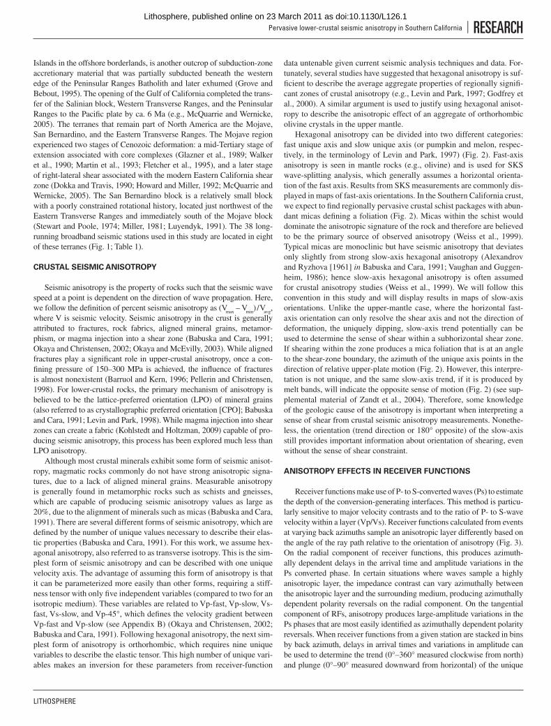
Receiver functions make use of P- to S-converted waves (Ps) to estimate the depth of the conversion-generating interfaces. This method is particu-larly sensitive to major velocity contrasts and to the ratio of P- to S-wave velocity within a layer (Vp/Vs). Receiver functions calculated from events at varying back azimuths sample an anisotropic layer differently based on the angle of the ray path relative to the orientation of anisotropy (Fig. 3). On the radial component of receiver functions, this produces azimuth-ally dependent delays in the arrival time and amplitude variations in the Ps converted phase. In certain situations where waves sample a highly anisotropic layer, the impedance contrast can vary azimuthally between the anisotropic layer and the surrounding medium, producing azimuthally dependent polarity reversals on the radial component. On the tangential component of RFs, anisotropy produces large-amplitude variations in the Ps phases that are most easily identifi ed as azimuthally dependent polarity reversals. When receiver functions from a given station are stacked in bins by back azimuth, delays in arrival times and variations in amplitude can be used to determine the trend (0°–360° measured clockwise from north) and plunge (0°–90° measured downward from horizontal) of the unique

as doi:10.1130/L126.1Lithosphere, published online on 23 March 2011

PORTER ET AL.

LITHOSPHERE

TAB

LE 1

. STA

TIO

N L

OC

AT

ION

S A

ND

INV

ER

SIO

N R

ES

ULT

S

Sta

tion

nam

eLa

titud

e(°

N)

Long

itude

(°W

)Te

cton

ic

bloc

kN

umbe

r of

R

Fs

used

in

inve

rsio

n

Laye

r 1

thic

knes

s (m

)

Ani

sotr

opic

la

yer

thic

knes

s (m

)

Laye

r 2

anis

otro

py(%

)

Ani

sotr

opy

tren

d(°

)

Ani

sotr

opy

plun

ge(°

)

Eta

Tim

e w

indo

w

star

t

Tim

e w

indo

w

stop

RM

S

mis

fi tTr

end

mis

fi tR

otat

ion

sinc

e 36

M

a (°

)

Rot

ated

an

isot

ropy

tr

end

BB

R34

.262

116.

921

SB

B20

026

,179

10,2

23–1

0.0

182

120.

752

35

0.04

02±

20

0.00

182.

00B

EL

34.0

0111

5.99

8E

TR

232

24,1

9865

30–1

1.1

606

0.72

82

50.

0192

± 2

045

.00

15.0

0B

FS

34.2

3911

7.65

9S

GB

194

25,5

4994

69–1

4.4

253

400.

658

25

0.03

02±

15

0.00

253.

00B

LA34

.070

116.

389

ET

R20

622

,650

13,0

39–1

8.5

129

810.

575

25

0.01

89±

50

45.0

084

.00

CH

F34

.333

118.

026

SG

B23

718

,651

9927

–16.

518

055

0.61

51.

55

0.02

86±

20

0.00

180.

00C

IA33

.402

118.

414

CB

L31

114

,456

8206

–14.

221

671

0.66

21

40.

0192

± 2

09.

2520

6.75

CIU

33.4

4611

8.48

3N

/A13

12,9

3989

61–7

.616

727

0.80

61

40.

0166

± 5

09.

2515

7.75

CR

Y33

.565

116.

737

PR

B55

423

,474

11,7

16–1

4.6

257

630.

654

25

0.02

11±

20

9.25

247.

75D

EC

34.2

5411

8.33

4W

TR

113

21,6

0211

,523

–20.

021

161

0.54

52

50.

0284

± 2

511

6.80

94.2

0D

JJ34

.106

118.

455

WT

R29

113

,507

12,7

49–1

6.6

162

0.61

31

50.

0186

± 2

011

6.80

244.

20E

DW

234

.881

117.

994

WM

B24

516

,599

10,6

70–1

2.7

177

460.

694

15

0.01

64±

20

0.00

177.

00F

MP

33.7

1311

8.29

4C

BL

9013

,022

7998

–20.

024

835

0.54

51

3.5

0.04

71±

15

9.25

238.

75G

SC

35.3

0211

6.80

6E

MB

465

19,0

2610

,238

–8.5

246

140.

786

15

0.01

82±

30

0.00

246.

00H

EC

34.8

2911

6.33

5E

MB

226

21,9

0692

63–1

0.7

268

220.

737

15

0.01

85±

40

0.00

268.

00JV

A34

.366

116.

613

EM

B18

523

,349

7514

–9.2

660

0.77

02

50.

0221

± 1

00.

0066

.00

KN

W33

.714

116.

712

PR

B48

810

,033

10,0

71–1

7.3

101

0.59

92

50.

0238

± 1

09.

250.

75LK

L34

.616

117.

825

WM

B21

19,0

3312

,300

–19.

015

668

0.56

52

50.

0156

± 5

00.

0015

6.00

MP

P34

.889

119.

814

SA

L14

423

,749

10,1

18–2

0.0

231

660.

545

25

0.02

44±

30

0.00

231.

00M

WC

34.2

2411

8.05

8S

GB

225

22,3

8511

,931

–20.

020

946

0.54

52

50.

0338

± 1

50.

0020

9.00

OS

I34

.615

118.

724

SG

B34

627

,382

6882

–15.

719

50

0.63

12

50.

0243

± 3

00.

0019

5.00

PA

S34

.148

118.

171

WT

R35

921

,888

8596

–10.

435

463

0.74

32

50.

0253

± 3

09.

2534

4.75

PA

SC

34.1

7111

8.18

5W

TR

7320

,244

7516

–18.

133

110

0.58

32

50.

0252

± 3

011

6.80

214.

20P

HL

35.4

0812

0.54

6S

AL

327

18,7

9275

73–8

.670

160.

783

14

0.01

97±

40

0.00

70.0

0P

KD

35.9

4512

0.54

2S

AL

277

24,0

6583

99–2

0.0

236

310.

545

25

0.04

11±

20

0.00

236.

00R

DM

33.6

3011

6.84

8P

RB

623

27,9

9882

84–5

.220

20

0.86

33

60.

0139

± 4

09.

2519

2.75

RP

V33

.744

118.

404

CB

L17

718

,469

8633

–20.

022

818

0.54

51

40.

0357

± 1

59.

2521

8.75

RR

X34

.875

116.

997

EM

B11

627

,990

8618

–20.

021

222

0.54

52

50.

0402

± 3

00.

0021

2.00

SB

PX

34.2

3211

7.23

5S

BB

175

28,0

0012

,278

–10.

831

456

0.73

53

60.

0202

± 5

00.

0031

4.00

SN

CC

33.2

4811

9.52

4N

/A34

10,9

1811

,338

–8.5

153

20.

786

24

0.01

84±

80

8.75

144.

25S

ND

33.5

5211

6.61

3P

RB

476

20,4

1611

,751

–11.

930

817

0.71

12

50.

0236

± 1

59.

2529

8.75

SV

D34

.107

117.

098

SB

B33

522

,604

14,9

46–1

0.2

118

60.

748

36

0.02

10±

50

9.25

108.

75T

OV

34.1

5611

8.82

0W

TR

239

26,0

8495

91–1

7.9

638

0.58

72

40.

0309

± 2

011

6.80

249.

20T

RO

33.5

2311

6.42

6P

RB

241

24,4

1059

06–1

1.8

247

320.

713

24

0.03

35±

20

9.25

237.

75T

UQ

35.4

3611

5.92

4E

MB

275

20,2

7793

59–9

.525

762

0.76

32

40.

0293

± 5

00.

0025

7.00

VC

S34

.484

118.

118

SG

B31

322

,754

10,9

11–7

.422

869

0.81

12

50.

0228

± 4

00.

0022

8.00

VT

V34

.561

117.

330

WM

B23

820

,698

9878

–9.2

134

430.

770

25

0.01

86±

25

0.00

134.

00W

MC

33.5

7411

6.67

5P

RB

369

25,5

3055

56–1

2.5

2837

0.69

82

40.

0331

± 1

09.

2518

.75

YA

Q33

.167

116.

354

PR

B13

811

,526

14,9

92–1

7.1

270

450.

603

24

0.02

93±

20

9.25

260.

75

Not

e: R

F—

Rec

eive

r fu

nctio

n; R

MS

—R

oot m

ean

squa

re. C

BL—

Con

tinen

tal B

orde

rland

; EM

B—

Eas

tern

Moj

ave

bloc

k; E

TR

—E

aste

rn T

rans

vers

e R

ange

s; P

RB

—P

enin

sula

r R

ange

s bl

ock;

SA

L—S

alin

ia; S

BB

—S

an B

erna

rdin

o bl

ock;

SG

B—

San

Gab

riel b

lock

; WM

B—

Wes

tern

Moj

ave

bloc

k; W

TR

—W

este

rn T

rans

vers

e R

ange

s.

as doi:10.1130/L126.1Lithosphere, published online on 23 March 2011

LITHOSPHERE

Pervasive lower-crustal seismic anisotropy in Southern California | RESEARCH

anisotropic axis for a given layer, as well as the percent anisotropy (e.g., Levin and Park, 1998; Sherrington et al., 2004; Ozacar and Zandt, 2009). While dipping layers and anisotropy can produce similar patterns in both the radial and tangential components, there are signifi cant differences in amplitude and delay patterns that make it possible to distinguish between the two. In particular, a dipping layer produces a zero-lag arrival on the tangential record section with a polarity reversal that is not observed for the anisotropy case (Fig. 3). Geologic constraints can also help distin-guish between dip and anisotropy. The presence of a consistent azimuthal pattern observed at several stations over a broad geographic area having structural complexity suggests a cause rooted in anisotropy, as opposed to a set of similarly dipping layers at the same depth.

To identify and parameterize seismic anisotropy, we fi rst calculate both radial and tangential receiver functions for each station within the study area. These are then visually examined for the aforementioned fea-tures, and time windows are selected that incorporate the Moho arrival and potential zones of lower-crustal anisotropy. Using this time window, a neighborhood algorithm search is conducted using the raysum forward modeling code (Frederiksen et al., 2003) to determine an anisotropic crustal model that best matches the observed signal. These results are then plotted and evaluated for error.

An important factor in describing hexagonal anisotropy is the elastic parameter η. The value of η defi nes the shape of the velocity ellipsoid between the P-fast and P-slow axes. For the inversion, we required that the velocity gradient between the P-fast and P-slow axes fi t a pure ellipse, following Levin and Park (1998). The rationale is explained in Appendix B. If we assume the gradient between the two velocities is a pure ellipse, η is function of the percent anisotropy, with higher percent anisotropies corresponding to lower η values for rocks with a slow unique axis. An η value equal to 1 describes an isotropic medium. Synthetic testing per-formed prior to the inversion demonstrated that variations in the value used to defi ne η have minimal impact on the inversion for trend of anisot-ropy, which is primarily dependent on the locations of polarity reversals and not relative amplitudes.

The calculated plunge of the unique axis of anisotropy and percent anisotropy are primarily dependent on the amplitude of arrivals and azimuthally dependent Ps delays observed in receiver functions. Varia-tions in both of these features can be relatively subtle in receiver func-tions and are sometimes hard to identify if the crust beneath a station has complicated structure. These diffi culties make the inversion for plunge and percent anisotropy less robust than the trend of the anisotropy. Varia-tions in anisotropy plunges near 0° are capable of producing 180° rota-tions in the calculated trend, and stations with plunges near 90° appear nearly isotropic in receiver functions. Station inversions that result in these extreme plunges are generally less accurate than inversions with a moderate plunge. Although slow unique axis anisotropy is assumed in this study, when the inversion was run assuming fast unique axis anisotropy, the best-fi tting model generally had a trend 180° and a dip 90° from the slow unique axis solution (Ozacar and Zandt, 2004). When synthetic RFs for both solutions were compared, the resulting move-out patterns were very similar and would be diffi cult, if not impossible, to differentiate in real data. Therefore, the most robust results from this study are the ori-entations of the trends, so we place the most emphasis on these in our interpretations.

DATA PROCESSING FOR RECEIVER FUNCTIONS

Receiver functions were computed from seismograms of teleseis-mic events between 25° and 95°, recorded on 38 Southern Californian broadband stations that were publicly available through the Incorporated Research Institutions for Seismology Data Management Center (IRIS DMC). Seismograms with a signal to noise ratio less than 3 were imme-diately discarded. The remaining traces were windowed from 10 s before to 100 s after the direct P-wave arrival and band-pass fi ltered using corner frequencies of 0.05 and 5 Hz. The seismograms were then down-sampled to 20 Hz, and the horizontal seismograms were rotated into radial and transverse components. An iterative time-domain deconvolution method (Ligorria and Ammon, 1999) with a Gaussian pulse width of 2.5, equiva-lent to a low-pass frequency of 1.2 Hz, was used to calculate the receiver functions. The calculated receiver functions were convolved with the vertical component trace and compared to the radial trace to assess the variance reduction, with higher values representing better deconvolutions.

Anisotropy ellipsoids

Anisotropic zone

Crust

Moho

Shear zone with aligned mineral grains (anisotropic)

Sense of shear

or

Shear zone with melt inclusion (anisotropic)

Magma injection

Mantle

A

Fast unique axis(melon) anisotropy

Slow unique axis(pumpkin) anisotropy

Unique velocity axes (slow)

B

Figure 2. (A) Cartoon diagram showing lower-crustal seismic anisotropy

and two ways shear zones can produce seismic anisotropy. The fi rst case

is caused by the alignment of mineral grains due to shear. The second

is the result of magma injections into a shear zone. (B) Anisotropy ellip-

soids showing the difference between fast and slow unique axis anisot-

ropy. For this work, slow unique axis anisotropy is assumed.

as doi:10.1130/L126.1Lithosphere, published online on 23 March 2011

PORTER ET AL.

LITHOSPHERE

45°

180°

Trend

Plunge

Anisotropyunique axis

N

Dipping layervelocity model

Dipping layerstrike and dip

N

20°

Slow axis

A

B

C

VpA>Vp

Bslow

VpA<Vp

Bfast

VpC>Vp

Bfast

VpC>Vp

Bslow

North

Anisotropic layer

Anisotropyvelocity model

Dipping layer

A

B

VpA>Vp

B

VpC>Vp

A

Positive polarity radial arrival

Negative polarity radial arrival

Negative polarity tangential arrival

Positive polarity tangential arrival

North

C

Negative polarity tangential arrival

Positive polarity tangential arrival

Positive polarity radial arrival

Negative polarity radial arrival

0 2 4 6 8

Bac

k az

imut

h (°

)

0

50

100

150

200

250

300

350

Time after P-wave (s)

Radial RadialTransverse Transverse

0 2 4 6 8 0 2 4 6 8 0 2 4 6 8

4 5 6 7 8

0

10

20

30

40

50

Vs–dashed; Vp−solid (km/s)

Dep

th (

km)

4 5 6 7 8

0

10

20

30

40

50

Vs–dashed; Vp−solid (km/s)

Dep

th (

km)

Figure 3. Diagram showing (upper left) a block of crustal rock with an isotropic dipping low-velocity layer (B) separating an isotropic crust (A) and

mantle (C) and (upper right) a block with a hypothetical lower-crustal anisotropic layer (B) located between an isotropic upper and middle crust (A)

and an isotropic mantle (C). The subvertical gray lines represent the ray paths for receiver functions sampling the layer. The fronts of the blocks show

the polarities of the radial components, while the right sides show the polarity of the tangential. The synthetic receiver functions correspond to the

associated crustal block. For both scenarios, assumed values are: crustal Vp of 6.4 km/s, a Vp/Vs of 1.75, and a Moho depth of 25 km. Mantle rocks are

assumed to have a Vp of 7.8 km/s and a Vp/Vs of 1.74. In the dipping layer example, a 5-km-thick 20°S-dipping layer with a Vp of 5.8 km/s is assumed.

In the anisotropic case, receiver functions were calculated assuming that seismic anisotropy is confi ned to a layer with a Vp of 6.2 km/s and 20%

anisotropy located in the bottom 5 km of the crust.

as doi:10.1130/L126.1Lithosphere, published online on 23 March 2011

LITHOSPHERE

Pervasive lower-crustal seismic anisotropy in Southern California | RESEARCH

After deconvolution, receiver functions were normalized to the radial component by dividing both components by the maximum radial value. Those with variance reductions of <0.80, with negative fi rst arrivals, or with extreme normalized amplitudes were discarded. Remaining receiver functions were plotted by back azimuth in bins of 20°. Each plotted bin contains the median value for all incoming rays with back azimuths ±10° of the bin value. Three stations had fewer than 35 RFs (CIU, LKL, SNCC); the rest had over 70, and a majority had between 200 and 623, which was the maximum number of RFs (Table 1). Previous studies of receiver functions in Southern California have focused on estimates of bulk crustal thickness and Vp/Vs (Zhu and Kanamori, 2000) and details of local and regional crustal structure (Yan and Clayton, 2007), but they have not considered the possibility of anisotropy. In this study, we focus on regional-scale lower-crustal anisotropy.

ANISOTROPY SEARCH PROCEDURE

Azimuthal plots of both the radial and transverse components of receiver functions for each station were examined for “indicators” of lower-crustal anisotropy. This was done by fi rst identifying the Moho Ps phase on the radial RFs and then inspecting the ~4 s window before the Moho arrival for phases that reversed polarity on the transverse component. For many of the Southern California stations, we were able to identify these diagnostic phases. In some cases, this was the major feature in the RFs, but for other stations, this lower-crustal signal was one of several layers of complex signal, both within the crust and in the upper mantle. With the focus of this study on lower-crustal anisotropy, we did not try to model the complete crustal structure for each station but rather restricted our efforts to estimating the anisotropic parameters for the basal crustal layer for all stations that displayed evidence of a potential anisotropic signal.

Synthetic receiver functions for an anisotropic medium were calcu-lated using a modifi ed version of the raysum code (Frederiksen and Bos-tock, 2000), a ray-based technique that calculates the amplitude and trav-eltimes for different phases, which are then combined to create a synthetic seismogram. The technique is limited to the plane-wave assumption, i.e., teleseismic waves, and is not applicable to models with steeply dipping layers (>50°) that potentially pinch out in the range of interest. We did not calculate multiples in our modeling because the multiples from the lower crust arrive much later than the time window with which we were concerned. In recorded data, multiples from localized shallow structures can potentially interfere with the arrivals in the time window of interest and produce variations in trend and anisotropic layer thickness. To miti-gate these local variations in results, we modeled several stations for each tectonic block and took the average anisotropy measurement for each block. The search code uses a global directed-search optimization tech-nique known as the neighborhood algorithm to solve for a set of given parameters (Frederiksen et al., 2003; Sambridge, 1999). The neighbor-hood algorithm search is summarized here and described in greater detail in Frederiksen et al. (2003) and Sambridge (1999). It works by randomly defi ning points in model space for several sets of free parameters (e.g.,

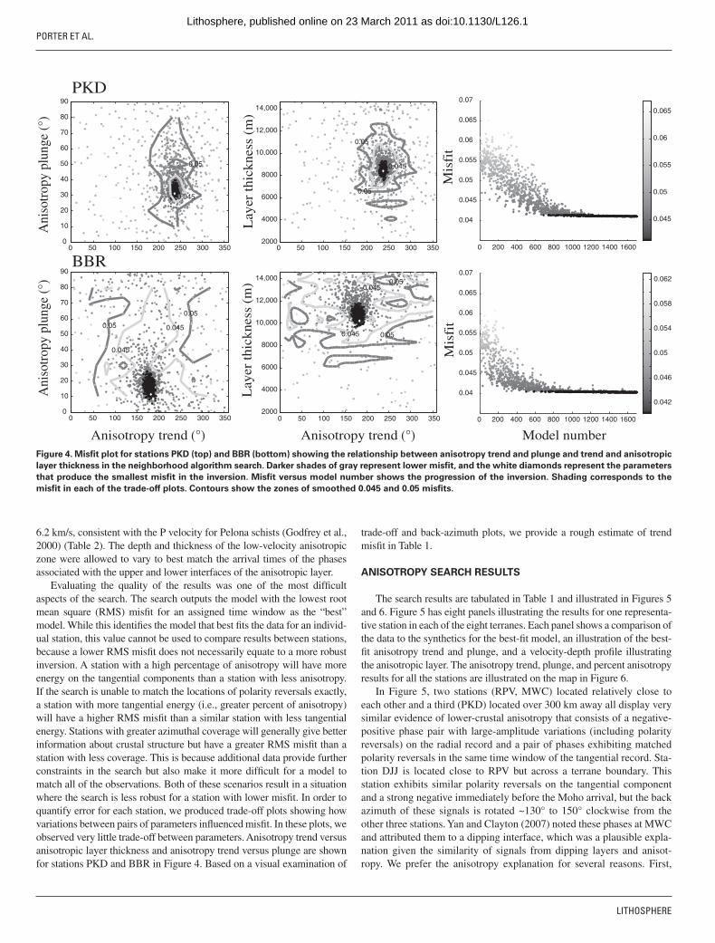
anisotropy trend, Moho depth, etc.; Table 2) and constructing polygons, known as neighborhoods, around each point. These polygons contain the point and all of the area in model space closest to that point that is not con-tained within another polygon. Misfi t between the observed and synthetic receiver functions is calculated for each point, and, once completed, more points are generated within the neighborhoods encompassing the points with the lowest misfi ts. New polygons are generated within the previous neighborhood for these new points, and the process is then repeated until a specifi ed number of iterations has been reached. The progression of the model misfi t is shown for stations PKD and BBR in Figure 4. For this work, we performed 20 iterations, searching 1700 models for each station. Experimenting with a few select stations demonstrated that increasing the number of iterations beyond 20 did not produce signifi cant improvement in misfi t or variations in results. We also modifi ed the original raysum inversion code by making the assumptions that the fi t between fast-and slow-velocity axes is a pure ellipsoid and that percent P and percent S anisotropy are equal. We found that without the pure ellipsoid constraint, it is possible to produce an anisotropic signal from a layer with 0% anisot-ropy when anisotropy is defi ned using η (Appendix B).

One of the advantages of the neighborhood algorithm search is that it will work for almost any method of calculating misfi t. We used an l

2

norm misfi t, which is more sensitive to amplitude and less sensitive to arrival time than the correlation misfi t (which is the default for the code; Frederiksen et al., 2003). The advantage of the l

2 norm is that it allows

us to easily calculate the misfi t for an assigned time window (Table 1), which gives us the ability to focus specifi cally on lower-crustal anisotropic zones. The parameters allowed to vary in the inversion were: anisotropic layer thickness, anisotropic layer depth, percent anisotropy, anisotropy slow-axis trend, and plunge. Density, the Vp/Vs ratio, P velocity, layer strike, and dip were all kept fi xed (Table 2).

For the search, we assumed that all of the tangential energy and azi-muthally dependent move-out was the result of seismic anisotropy and not dipping layers. While this assumption oversimplifi es the crustal structure, allowing for both dipping layers and anisotropy results in a less effi cient search. To test this assumption, searches were run on select stations allow-ing for layers that were both anisotropic and dipping. The results from these tests showed that allowing both parameters to vary did not measur-ably improve the fi t to the data (see GSA Data Repository supplement1). To determine if the observed signal was a result of dipping layers, searches were done on these same stations but allowing for dipping layers with no anisotropy; however, these results did not fi t the data as well as those that assumed seismic anisotropy (see GSA Data Repository supplement [see footnote 1]). In the search for anisotropy, we assumed that the crust consisted of an upper-crustal layer with a P-wave velocity of 6.4 km/s and an anisotropic lower-crustal low-velocity layer with an average velocity of

1GSA Data Repository Item 2011138, results showing the effects of inverting receiver-function data assuming anisotropy, a dipping layer, and anisotropy and a dipping layer, is available at www.geosociety.org/pubs/ft2011.htm, or on request from editing@geosociety.org, Documents Secretary, GSA, P.O. Box 9140, Boulder, CO 80301-9140, USA.

TABLE 2. INVERSION PARAMETERS AND THEIR RANGES

Layer Thickness(m)

Density(kg/m3)

P velocity(m/s)

Vp/Vs Isotropic % anisotropy Anisotropy trend(°)

Anisotropy plunge(°)

Strike Dip

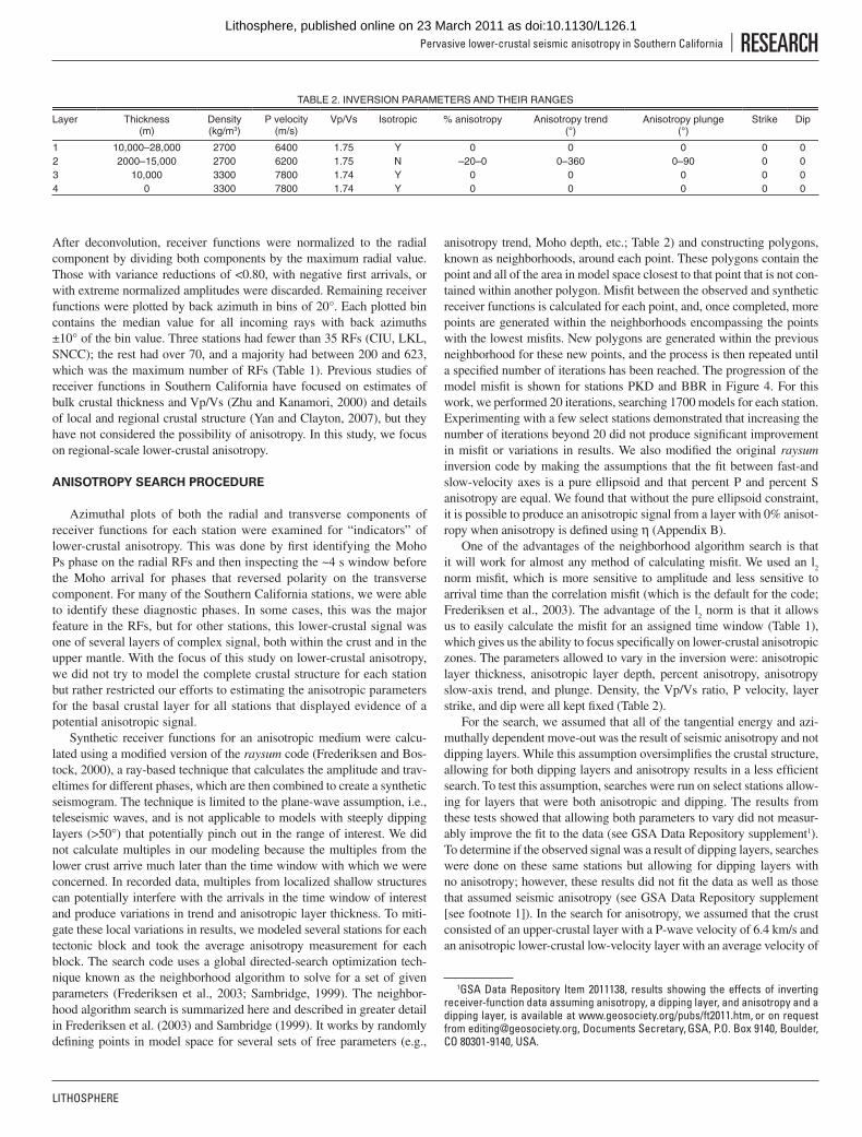
00000Y57.100460072000,82–000,0112 2000–15,000 2700 6200 1.75 N –20–0 0–360 0–90 0 0

00000Y47.100870033000,01300000Y47.10087003304

as doi:10.1130/L126.1Lithosphere, published online on 23 March 2011

PORTER ET AL.

LITHOSPHERE

6.2 km/s, consistent with the P velocity for Pelona schists (Godfrey et al., 2000) (Table 2). The depth and thickness of the low-velocity anisotropic zone were allowed to vary to best match the arrival times of the phases associated with the upper and lower interfaces of the anisotropic layer.

Evaluating the quality of the results was one of the most diffi cult aspects of the search. The search outputs the model with the lowest root mean square (RMS) misfi t for an assigned time window as the “best” model. While this identifi es the model that best fi ts the data for an individ-ual station, this value cannot be used to compare results between stations, because a lower RMS misfi t does not necessarily equate to a more robust inversion. A station with a high percentage of anisotropy will have more energy on the tangential components than a station with less anisotropy. If the search is unable to match the locations of polarity reversals exactly, a station with more tangential energy (i.e., greater percent of anisotropy) will have a higher RMS misfi t than a similar station with less tangential energy. Stations with greater azimuthal coverage will generally give better information about crustal structure but have a greater RMS misfi t than a station with less coverage. This is because additional data provide further constraints in the search but also make it more diffi cult for a model to match all of the observations. Both of these scenarios result in a situation where the search is less robust for a station with lower misfi t. In order to quantify error for each station, we produced trade-off plots showing how variations between pairs of parameters infl uenced misfi t. In these plots, we observed very little trade-off between parameters. Anisotropy trend versus anisotropic layer thickness and anisotropy trend versus plunge are shown for stations PKD and BBR in Figure 4. Based on a visual examination of

trade-off and back-azimuth plots, we provide a rough estimate of trend misfi t in Table 1.

ANISOTROPY SEARCH RESULTS

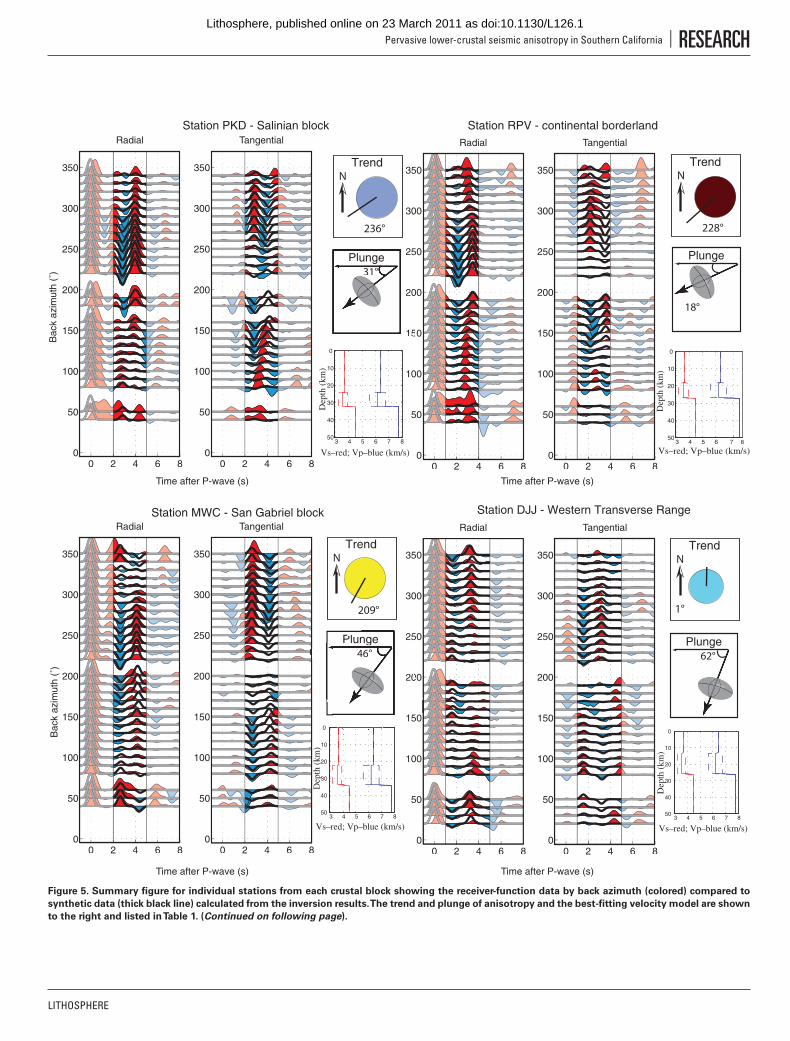
The search results are tabulated in Table 1 and illustrated in Figures 5 and 6. Figure 5 has eight panels illustrating the results for one representa-tive station in each of the eight terranes. Each panel shows a comparison of the data to the synthetics for the best-fi t model, an illustration of the best-fi t anisotropy trend and plunge, and a velocity-depth profi le illustrating the anisotropic layer. The anisotropy trend, plunge, and percent anisotropy results for all the stations are illustrated on the map in Figure 6.

In Figure 5, two stations (RPV, MWC) located relatively close to each other and a third (PKD) located over 300 km away all display very similar evidence of lower-crustal anisotropy that consists of a negative-positive phase pair with large-amplitude variations (including polarity reversals) on the radial record and a pair of phases exhibiting matched polarity reversals in the same time window of the tangential record. Sta-tion DJJ is located close to RPV but across a terrane boundary. This station exhibits similar polarity reversals on the tangential component and a strong negative immediately before the Moho arrival, but the back azimuth of these signals is rotated ~130° to 150° clockwise from the other three stations. Yan and Clayton (2007) noted these phases at MWC and attributed them to a dipping interface, which was a plausible expla-nation given the similarity of signals from dipping layers and anisot-ropy. We prefer the anisotropy explanation for several reasons. First,

0

10

20

30

40

50

60

70

80

90

0 50 100 150 200 250 300 350

2000

4000

6000

8000

10,000

12,000

14,000

0 50 100 150 200 250 300 350

0.05

0.045

0.05

0.04

0.045

0.05

0.055

0.06

0.065

0.07

0.045

0.05

0.055

0.06

0.065

Mis

fit

0 200 400 600 800 1000 1200 1400 1600

2000

4000

6000

8000

10,000

12,000

14,000

0 50 100 150 200 250 300 350

0.050.045

0.050.045

0 200 400 600 800 1000 1200 1400 1600

0.04

0.045

0.05

0.055

0.06

0.065

0.07

0.042

0.046

0.05

0.054

0.058

0.062

Mis

fit

0 50 100 150 200 250 300 3500

10

20

30

40

50

60

70

80

90

0.05

0.05 0.045

0.045

Ani

sotr

opy

plun

ge (°

)

Model numberAnisotropy trend (°)

Lay

er th

ickn

ess

(m)

Ani

sotr

opy

plun

ge (°

)

Anisotropy trend (°)

Lay

er th

ickn

ess

(m)

0.05

0.045

PKD

BBR

Figure 4. Misfi t plot for stations PKD (top) and BBR (bottom) showing the relationship between anisotropy trend and plunge and trend and anisotropic

layer thickness in the neighborhood algorithm search. Darker shades of gray represent lower misfi t, and the white diamonds represent the parameters

that produce the smallest misfi t in the inversion. Misfi t versus model number shows the progression of the inversion. Shading corresponds to the

misfi t in each of the trade-off plots. Contours show the zones of smoothed 0.045 and 0.05 misfi ts.

as doi:10.1130/L126.1Lithosphere, published online on 23 March 2011

LITHOSPHERE

Pervasive lower-crustal seismic anisotropy in Southern California | RESEARCH

0 2 4 6 80

50

100

150

200

250

300

350

Tangential

0 2 4 6 80

50

100

150

200

250

300

350

Radial

0 2 4 6 80

50

100

150

200

250

300

350

Tangential

0 2 4 6 80

50

100

150

200

250

300

350

Radial

0 2 4 6 80

50

100

150

200

250

300

350

Tangential

0 2 4 6 80

50

100

150

200

250

300

350

Radial

0 2 4 6 80

50

100

150

200

250

300

350

Tangential

0 2 4 6 80

50

100

150

200

250

300

350

Radial

Station PKD - Salinian block Station RPV - continental borderland

Station MWC - San Gabriel block Station DJJ - Western Transverse Range

31°

Plunge

15

20

2

31°

Plunge

3 4 5 6 7 8

0

10

20

30

40

50

Vs–red; Vp–blue (km/s)

Dep

th (

km)

N

236°

Trend

3 4 5 6 7

0

10

20

30

40

50

Dep

th (

km)

8

Vs–red; Vp–blue (km/s)

18°

Plunge

N

228°

Trend

3 4 5 6 7 8

0

10

20

30

40

50

Vs–red; Vp–blue (km/s)

Dep

th (

km)

46°

Plunge

150

20

46°

Plunge

N

209°

Trend

62°

Plunge

N

1°

Trend

3 4 5 6 7 8

0

10

20

30

40

50

Vs–red; Vp–blue (km/s)

Dep

th (

km)

Bac

k az

imut

h (˚

)B

ack

azim

uth

(˚)

Time after P-wave (s)Time after P-wave (s)

Time after P-wave (s)Time after P-wave (s)

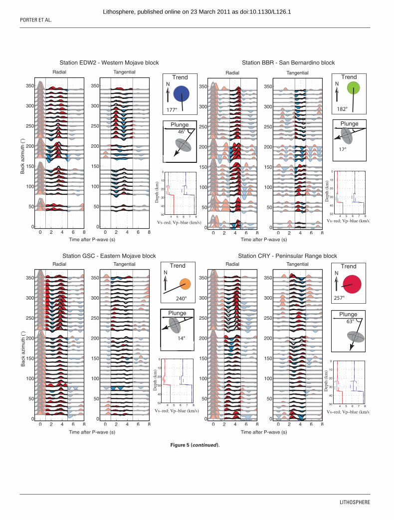
Figure 5. Summary fi gure for individual stations from each crustal block showing the receiver-function data by back azimuth (colored) compared to

synthetic data (thick black line) calculated from the inversion results. The trend and plunge of anisotropy and the best-fi tting velocity model are shown

to the right and listed in Table 1. (Continued on following page).

as doi:10.1130/L126.1Lithosphere, published online on 23 March 2011

PORTER ET AL.

LITHOSPHERE

46°

Plunge46°

Plunge

N

177°

Trend

12°

Plunge

N

182°

Trend

14°

Plunge

14°

Plunge

N

240°

Trend

63°

Plunge

N

257°

Trend

0 2 4 6 80

50

100

150

200

250

300

350

Tangential

0 2 4 6 80

50

100

150

200

250

300

350

Radial

0 2 4 6 80

50

100

150

200

250

300

350

Tangential

0 2 4 6 80

50

100

150

200

250

300

350

Radial

0 2 4 6 80

50

100

150

200

250

300

350

Tangential

0 2 4 6 80

50

100

150

200

250

300

350

Radial

0 2 4 6 80

50

100

150

200

250

300

350

Tangential

0 2 4 6 80

50

100

150

200

250

300

350

Radial

Station BBR - San Bernardino block

Station CRY - Peninsular Range block

Station EDW2 - Western Mojave block

Station GSC - Eastern Mojave block

4 5 6 7 8

0

10

20

30

40

50

Vs–red; Vp–blue (km/s)

Dep

th (

km)

4 5 6 7 8

0

10

20

30

40

50

Vs–red; Vp–blue (km/s)

Dep

th (

km)

4 5 6 7 8

0

10

20

30

40

50

Vs–red; Vp–blue (km/s)

Dep

th (

km)

4 5 6 7 8

0

10

20

30

40

50

Vs–red; Vp–blue (km/s)

Dep

th (

km)

Bac

k az

imut

h (˚

)B

ack

azim

uth

(˚)

Time after P-wave (s)Time after P-wave (s)

Time after P-wave (s)Time after P-wave (s)

12°

Plunge

Figure 5 (continued ).

as doi:10.1130/L126.1Lithosphere, published online on 23 March 2011

LITHOSPHERE

Pervasive lower-crustal seismic anisotropy in Southern California | RESEARCH

the comparison of a dipping versus an anisotropy layer illustrated in Figure 3 shows that the dipping layer case has a diagnostic arrival on the tangential record of a polarity reversing phase at zero lag time (centered at time zero), which is absent for the anisotropy case. The zero lag phase is not observed at MWC or at the other stations, although some shal-lower phases are present. A more subtle difference is that the anisotropy case has polarity reversals on the radial component that are not observed in the dipping layer case, and again polarity reversals are observed on the radial data from MWC and other stations. Perhaps most signifi cant to us is the similarity of signals from both closely spaced and distant stations. This would either require similarly dipping interfaces at similar depths beneath all these stations or a similar anisotropic layer. Given the geologic evidence for the presence of underplated schists beneath all these stations, we prefer the anisotropy explanation.

The linear nature of the trend versus plunge and trend versus layer thickness in trade-off plots (samples shown in Fig. 4) demonstrates that the inversion for anisotropy trend is more stable relative to other parameters. This is because trend is determined by the location of polarity reversals, which are relatively easy to locate within the tangential record section. Calculated percent anisotropy values for the region are generally higher than expected for crustal rocks and are relatively less constrained in the inversion. The high percent anisotropy values might be explained in part by unmodeled near-surface low-velocity zones (i.e., basins) that refract

the incoming P-wave arrival to vertical, effectively changing the relative amplitudes of the converted (Ps) waves compared to the direct (P) wave on the radial RF component. Forward modeling of receiver functions with a 5 km low-velocity zone at the top of the crust, and then inversion of the results for anisotropy without a low-velocity upper-crustal layer, produces high percent anisotropy values for crustal rocks.

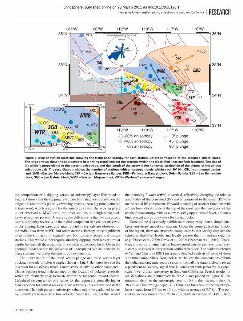
Some of the data clearly exhibit more complexity than a simple one-layer anisotropy model can explain. Given the complex tectonic history of the region, there are structural complications that locally emplace the schists at shallower levels, and locally expose them in surface outcrops (e.g., Ducea et al., 2009; Grove et al., 2003; Chapman et al., 2010). There-fore, it is not surprising that the lower-crustal anisotropic layer is not con-sistently observed at every station within each block. The reader is referred to Yan and Clayton (2007) for a more detailed analysis of some of these structural complexities. Nonetheless, we believe that comparisons of both the radial and tangential record sections from all the stations clearly reveal a persistent anisotropy signal that is consistent with pervasive regional-scale lower-crustal anisotropy in Southern California. Search results for all 38 stations are summarized in Table 1 and plotted in Figure 6. The minimum depth to the anisotropic layer is 10 km, the maximum depth is 28 km, and the average depth is ~21 km. The thickness of the anisotropic layer ranges from 5.5 km to 15 km, with an average of 9.7 km. The per-cent anisotropy ranges from 5% to 20%, with an average of ~14%. The η

-121°

121°W

-120°

120°W

119°W

119°W

118°W

118°W

117°W

117°W

116°W

116°W

33° 33°N

34°N 34°N

35°N 35°N

36°N 36°N

-20% anisotropy-10% anisotropy

0% anisotropy

0° plunge45° plunge90° plunge

RRX

BBR

BEL

BLA

CIA

CIU CRY

DEC

DJJ

EDW2

FMP

GSC

HEC

JVA

KNW

LKL

MPP

PASPASC

PHL

PKD

RDM

RPV

SBPX

SNCC

SND

SVDTOV

TRO

TUQ

VTV

WMC

YAQ

CHF

MWC

OSI

VCS

BFS

EMBWMB

PRB

ETR

SBB

SAL

WTR

CBL

SGB

119°W

119°W

118°W

118°W

117°W

117°W

34°N 34°N

35°N 35°N

RRX

DEC

DJJ

LKL

PASPASC

SBPX

SVDTOV

VTV

CHFMWC

VCS

BFS

WMBEDW2

OSI

WTRSGB

90°270°

180°

Unique axis distribution by azimuth

1 station

3 stations

Figure 6. Map of station locations showing the trend of anisotropy for each station. Colors correspond to the assigned crustal block.

The large arrows show the approximate best-fi tting trend lines for the stations within the block. Red lines are fault locations. The size of

the circle is proportional to the percent anisotropy, and the length of the arrow is the horizontal projection of the plunge of the unique

anisotropic axis. The rose diagram shows the number of stations with anisotropy trends within each 10° bin. CBL—continental border-

land; EMB—Eastern Mojave block; ETR—Eastern Transverse Ranges; PRB—Peninsular Ranges block; SAL—Salinia; SBB—San Bernardino

block; SGB—San Gabriel block; WMB—Western Mojave block; WTR—Western Transverse Ranges.

as doi:10.1130/L126.1Lithosphere, published online on 23 March 2011

PORTER ET AL.

LITHOSPHERE

values range from 0.545 to 0.863, with an average of 0.664. Of the 38 sta-tions that we inverted for anisotropy, 34 were used to calculate the regional anisotropy trend and the average anisotropy for the tectonic blocks. The anisotropy calculations for the remaining four stations (shaded white in Fig. 1) were not included in the fi nal interpretation because they either did not lie within one of the defi ned tectonic blocks or else did not have signifi cant azimuthal coverage to produce robust anisotropy results.

ANISOTROPY RESULTS BY CRUSTAL TERRANE

The rose diagram in Figure 6 illustrates the distribution of the trend directions. A regional-scale anisotropic trend is present in the area with a best-fi tting unique axis orientation of 211° and a standard deviation of 43° (assuming orientations 180° apart are equivalent), calculated for the 34 stations assigned to tectonic blocks. The signifi cant scatter in the results can be partially explained by separating the results into groups sampling the different geologic/tectonic blocks that constitute the crust in the region. As we demonstrate next, anisotropy results within each crustal block appear to be more coherent.

Salinian Block

The Salinian terrane is a large composite terrane (see Appendix A), and three stations are not nearly enough for a complete characterization. Nonetheless, the three stations in southern Salinia that we examined have a common SW-NE azimuth of anisotropy. Two stations (PKD and MPP) exhibit nearly identical trends of 231° and 236°, and the other (PHL) sta-tion has a nearly opposite trend of 70°. PHL has a relatively weak sig-nal and small magnitude of percent anisotropy (−9%) compared to the other two stations (−20%). Rotating station PHL’s unique anisotropy axis 180° to 250° results in an average unique axis orientation of ~239° for the block, with a standard deviation of ~10°. The ~239° trend agrees within estimated error with the detailed study by Ozacar and Zandt (2009) for the Parkfi eld station, PKD. They interpreted the anisotropy observed at this station as a fossil fabric from Farallon subduction in either a serpenti-nite layer or a fl uid-fi lled schist layer, based on the high Vp/Vs calculated for the lower crust. The underplated schist interpretation is supported by new fi eld evidence suggesting that the Salinian block is largely a remnant Cretaceous arc underplated by schists, similar to those that outcrop in the Sierra de Salinas (Kidder and Ducea, 2006; Chapman et al., 2010). The opposite orientation of PHL compared to PKD and MPP might be attrib-uted to large-magnitude extension of the underplated schists following fl at slab subduction (Chapman et al., 2010). The composition of the schists indicates that the most anisotropic mineral preserved in the outcrop is mica (Ducea et al., 2007). Regardless of the exact source of the anisotropy, the orientation of the slow axis approximately orthogonal to the trend of the San Andreas fault at this location suggests that northwestward transla-tion of the Salinian block along the San Andreas fault is not deforming the lower crust in a way that modifi es the observed lower-crustal anisotropy.

San Gabriel Block

The San Gabriel block is much smaller than the Salinian block, and so the stations located within it provide a much better sampling of this terrane. The anisotropy trend measurements for the fi ve stations clearly in the San Gabriel block average out to ~213°, with a standard devia-tion of ~29°, which is nearly the same direction as for the Salinian block, within error. In this case, all the trends are oriented to the SW, although measurements from station OSI are affected by structural complexities. Station DEC, which is located very close to the boundary between the

Western Transverse Ranges and the San Gabriel block, exhibits a trend of 211°, which is consistent with the San Gabriel block results. Though located in the Western Transverse Ranges in the reconstruction, given the uncertainly of the terrane boundaries at depth, we argue that in future work DEC should be grouped with the San Gabriel block terrane, resulting in a more consistent reconstruction. The San Gabriel block is composed of Mesozoic and Proterozoic igneous and metamorphic rocks thrust over the Pelona Schist (Jacobson, 1983). Based on the reconstruction of McQuar-rie and Wernicke (2005), the block has not undergone signifi cant rotation. The similarity of the geologic history of the terranes suggests to us that the similar anisotropy results are due to a common cause: the subduction emplacement of schists beneath these terranes.

Western Transverse Ranges

Much of the Western Transverse Ranges terrane is located offshore, so the stations we have in this terrane only sample a small portion of its east-ernmost end. The results for the four stations clearly in the Western Trans-verse Ranges are distinctly different from the results in the Salinian and San Gabriel blocks, with an average trend of 353° or approximately north.

The Western Transverse Ranges have a complex deformational history of translations, rotations, and shortening (Appendix A). One possibility is that the N-S orientation of anisotropy trend refl ects the >260 km of northward translation of the terrane since the early Miocene. However, other neighboring terranes outboard of the San Andreas fault have experi-enced similar translations and do not show the northward trend. It is also possible that anisotropy measurements refl ect lower-crustal shear traction within the Western Transverse Ranges, which contain numerous indica-tors of intense N-S shortening (J. Saleeby, 2010, personal commun.). Unlike many of its neighboring terranes, the Western Transverse Ranges block has also undergone >100° of clockwise rotation since the early Mio-cene (Luyendyk, 1991). If rotated back 116° counterclockwise to its pre-Miocene orientation, the average anisotropy trend for the four N-oriented stations is 237°, aligning it with our “subduction accretion” trend. Given the diffi culty in determining the cause of anisotropy for the block, we con-clude that active tectonics and schist emplacement are both viable options.

Continental Borderland

Godfrey et al. (2002) argued that the crust within the inner continen-tal borderland is composed of Catalina schist underlain by a greenschist-facies basaltic rock, interpreted as a fossilized subduction zone. The stations in this predominantly submerged terrane are confi ned to the far eastern part of this province, making it diffi cult to establish the anisotropic signal for the entire crustal block. The three higher-quality results we have show an average anisotropy trend of ~231° with a standard deviation of ~16°, again the subduction accretion trend. Two lower-quality results indi-cate a more N-S trend, which may be due to the strong extension in this region that followed in the wake of the rotation of the Western Transverse Ranges. Similar to the Western Transverse Ranges, the few observations we have from this large terrane are consistent with either active tectonics or schist emplacement.

Peninsular Ranges Block

The Peninsular Ranges block is composed of relatively intact batho-lithic crust, and its transfer to the Pacifi c plate in the past 6 m.y. as a cohesive body strongly suggests that it still retains a portion of its mantle lithosphere (J. Saleeby, 2010, personal commun.). The seven stations we analyzed in the Peninsular Ranges block are located in a relatively

as doi:10.1130/L126.1Lithosphere, published online on 23 March 2011

LITHOSPHERE

Pervasive lower-crustal seismic anisotropy in Southern California | RESEARCH

confi ned area of the northern Peninsular Ranges block. The anisotropy trends calculated for the Peninsular Ranges show the most variability among the terranes we examined, ranging from WSW to NNE. Within the region, station RDM exhibited an extremely weak anisotropic signa-ture, and the Moho is not a clear consistent arrival at KNW. Two stations, WMC and SND, located close to each other and near the trace of the San Jacinto fault display widely disparate results, perhaps refl ecting complexi-ties related to the fault. Three stations, CRY, TRO, and YAQ, display a more consistent WSW trend, and station KNW has an anomalous N trend.

The 10° dip in the Moho identifi ed by Lewis et al. (2000) could impact the results from these stations. To test this possibility, searches were run for anisotropy assuming a 10° dipping Moho. The results did not change signifi cantly (<15°) for all but two of the stations, suggesting that the impact of this dip on our anisotropy trends is minimal. The proximity of most of the stations in this block to active fault strands may explain the variability of the observed anisotropy trends.

Mojave Block (Western and Eastern)

On the North American side of the San Andreas fault, we have results for the large Mojave terrane and the smaller San Bernardino block. Due to variations across the Eastern California shear zone, the Mojave was divided into two blocks: the eastern and western Mojave blocks. Three stations exhibit a SSE orientation of anisotropy in the west, and four sta-tions exhibit a WSW trend in the east. The three western Mojave stations have an average anisotropy azimuth of ~156°, with a standard deviation of 22°, while the fi ve eastern Mojave stations average ~246°, with a stan-dard deviation of 21°, when the unique anisotropy azimuth for station JVA is rotated 180°. Within the Mojave, station LKL has relatively poor azimuthal coverage, and stations in the eastern Mojave all exhibit effects from complicated crustal structure, potentially impacting our inversion results. In general, stations in the Mojave exhibit a weaker anisotropic signal with less energy on the tangential component of receiver func-tions than is observed west of the San Andreas fault, making the inversion results for this area less robust.

Luffi et al. (2009) and Chapman et al. (2010) argued that much of the western Mojave experienced the same subduction erosion and schist underplating that occurred throughout the rest of Southern California. Thus, one would expect a similar direction of anisotropy (~240°) as other terranes that preserve this signal. The opposing trend observed at JVA may have the same explanation as we proposed for PHL in the Salinian block, that is, it may refl ect extrusion of the underplated schists (Chapman et al., 2010). The anisotropy azimuth of ~156° calculated for the western Mojave suggests that the lower-crustal anisotropy trend appears to have been reset by younger deformational events. We will reevaluate the Mojave interpre-tation after the tectonic reconstruction later in this paper.

San Bernardino Block

This small crustal block is part of the Transverse Ranges; however, the bedrock of the San Bernardino block is most strongly correlated to the immediately adjacent Mojave basement near Victorville (Stew-art and Poole, 1974; Miller, 1981). Like the western Mojave, the San Bernardino block upper crust is underlain by schist, interpreted to be the Orocopia schist by Powell (1981). Two of the stations display S-SE trends, while a third has a NW trend. One station, SVD, is located between two branches of the active San Andreas fault, and, interestingly, it exhibits a fault-parallel trend. In some ways, the trends in this small block appear similar to those observed in the western Mojave block just to the north. However, the receiver functions from these stations are rela-

tively complex, making these results less robust than those from other crustal blocks.

TECTONIC RECONSTRUCTION TO 36 Ma

In order to develop a better picture of the relative locations and orienta-tions of the anisotropy trends to pretransform paleogeography, the crustal blocks with their seismic stations were restored back to their early Oligo-cene (36 Ma) positions and orientations, based on the reconstruction of McQuarrie and Wernicke (2005) (Fig. 7). The anisotropy locations and rotations were palinspastically restored by associating each of the individ-ual points with the polygons reconstructed by McQuarrie and Wernicke (2005). Points were then restored via incremental translation and rotation about their associated polygon centroid (McQuarrie and Oskin, 2010) (Table 1). The 36 Ma time frame was chosen not only because it is the earliest time frame in the reconstruction, but also because it takes us back to a pretransform period, when subduction was active along the entire coastline. Restoring the anisotropy highlighted subtle problem areas in the tectonic reconstruction of McQuarrie and Wernicke (2005). The geologi-cal boundaries of the reconstruction are based on geographic information system (GIS) polygons from the 1:5,000,000 scale tectonic map of Mue-hlberger (1996). Given the complexity of Southern California tectonic his-tory, there are a variety of interpretations in the restored locations of crustal blocks. While this is a signifi cant issue, our interpretation is primarily dependent on the rotational history of the blocks; as such, uncertainties in restored locations are less important than those related to orientation. The scale of the map used to defi ne geologic boundaries is such that station locations in close proximity to polygon boundaries may be assigned to the wrong block. As an example of a potential boundary problem, stations PAS and PASC are located ~3 km apart, yet they palinspastically relocate to widely separated locations. In this reconstruction, station PAS is located on the northernmost edge of the Peninsular Range polygon, which did not experience signifi cant rotation. Immediately adjacent is station PASC, in the Western Transverse Ranges, which underwent 116° of rotation. Pre-restoration PAS and PASC stations record similar anisotropies of 354° and 332°, respectively. When palinspastically rotated 116°, station PASC matches the other Western Transverse Ranges anisotropies as well as the overall SW-trending anisotropy of the region (Fig. 7); however, PAS, with little rotation but signifi cant translation with the Peninsular Range block, does not. This suggests that both PAS and PASC should be restored with the Western Transverse Ranges. As discussed earlier, station DEC, while reconstructed on the northern edge of the Western Transverse Ranges terrane, has the anisotropic signature of the adjacent San Gabriel block, which shows a SW-trending anisotropy before rotation (Fig. 6). After the rotation of the Western Transverse Ranges block, the anisotropy of DEC dips to the east (Fig. 7), confi rming it should be restored with the San Gabriel block. The reconstruction does not answer all questions regarding the San Bernardino block, but it does provide some insight into the aniso-tropic signal there. This block has a relatively unconstrained rotational history and exhibits complicated receiver-function signals observed at the stations within it. Given the proximity of stations SBPX and SVD to the San Andreas fault at 36 Ma, it is possible to attribute the anisotropy trends observed at these stations to deformation associated with motion along the fault. Within the block, post-subduction deformation could obscure the anisotropic signal directly related to underplated schist. Station SVD is located between two strands of the San Andreas fault and is assigned to a polygon that has signifi cant southward translation in the reconstruction. Given its location, it is unclear if SVD should be included within the San Bernardino block. Stations with uncertain locations in the reconstruction are transparent on the map and are not included in the rose diagram of the

as doi:10.1130/L126.1Lithosphere, published online on 23 March 2011

PORTER ET AL.

LITHOSPHERE

post-restoration trend distribution nor were they considered in calculating best-fi tting anisotropy arrows for the tectonic blocks (Fig. 7).

Comparing the rose diagrams of anisotropy trends prior to and after restoration (Figs. 6 and 7), we observe a signifi cant tightening in the azi-muthal distribution. The dominant trend is at ~240°, with a much smaller peak in the opposite direction of ~60°. This orientation coincides closely with the Farallon–North American convergence direction for the end of the Laramide (ca. 59–42 Ma) (Saleeby, 2003). Subordinate peaks occur for N-S and NW-SE orientations.

In the map view of the 36 Ma reconstruction, stations in blocks origi-nally west of the San Andreas fault (Salinian block, San Gabriel block, Western Transverse Ranges, and Peninsular Ranges block) all exhibit sim-ilar SW-NE orientations, and predominantly SW trends, consistent with a top-to-SW sense of shear, assuming an S-C–type cause for the anisot-ropy. This is consistent with the hypothesis of subduction emplacement of schists derived from the accretionary complex.

While the tectonic reconstruction of McQuarrie and Wernicke (2005) is based on >100 unique displacement constraints for the reconstruction

east of the San Andreas fault, displacements of fault-bounded blocks west of the San Andreas fault are only controlled by fi ve, fi rst-order constraints. These are (1) displacement on the San Andreas fault (Matthews, 1976; Graham et al., 1989; Dickinson, 1996), (2) ~110° clockwise rotation of the Western Transverse Ranges (Hornafi us et al., 1986; Luyendyk, 1991), (3) attenuation of the continental borderlands in the wake of the rotat-ing Transverse Ranges (Crouch and Suppe, 1993; Bohannon and Geist, 1998), (4) opening of the Gulf of California (Oskin et al., 2001; Oskin and Stock, 2003), and (5) the easternmost extent of Pacifi c plate oceanic crust, which constrains the maximum western extent of continental North America (Atwater and Stock, 1998). By taking into account only these fi rst-order constraints, the attempt at a self-consistent, strain-compatible model highlights several problems, many of which are focused along and west of the San Andreas system (McQuarrie and Wernicke, 2005). One of these problems, directly related to this study, is the restoration of the coastal Salinia terrane to a position that overlaps with the western Mojave Desert. This kinematic incompatibility (see Chapman et al., 2010) arises from the requirement that continental crust cannot be west of the restored

HEC

BLA

EDW2

RRX

JVA

PHL

BELJVA

PAS

KNW

WMCRDM

TRO

YAQ

CRY

SND

CIACIU

RPV

FMP

SVD

MPP

OSI

TUQ

TOV

BFS

VCS

CHF

MWC

LKL

GSC

BBRSBPX

PKD VTV

DEC PASC

DJJ

Sierra Nevada

Great Valley

Mojave

0 150 30075

km

Southern California36 Ma

M

90°270°

180°

0°Unique axis distribution by azimuth

2 stations4 stations

ColoradoPlateau

Edg

e of early Tertiary exten

sion

Salinia

SGT

Peninsular

Ranges

FutureSan Andreas fault

futureGarlock fault

Southern California borderland forearc basin

Franciscan

sub

du

ction

com

plex

WTR

Farallon:North Americarelative motion

vectors 59−50 Ma

50−42 Ma

Tectonicerosionaledge of

Salinia

Figure 7. Map of station locations

and unique anisotropy axis ori-

entations at 36 Ma based on the

reconstruction of McQuarrie and

Wernicke (2005). Station coloring

corresponds to the crustal blocks.

The large arrows show the best-

fi tting block trend lines rotated

back to their orientation at 36 Ma.

Stations SVD and PAS are not

included in the block averages

shown by the large arrows and in

the rose diagram. Transparent sta-

tions are “problem” stations iden-

tifi ed in the text. The rose diagram

shows the number of stations

with anisotropy trends within

each 10° bin when rotated back

to their 36 Ma orientations. Vec-

tors show early Tertiary Farallon–

North America relative motion

vectors from Saleeby (2003).

SGB—San Gabriel block; WTR—

Western Transverse Ranges.

as doi:10.1130/L126.1Lithosphere, published online on 23 March 2011

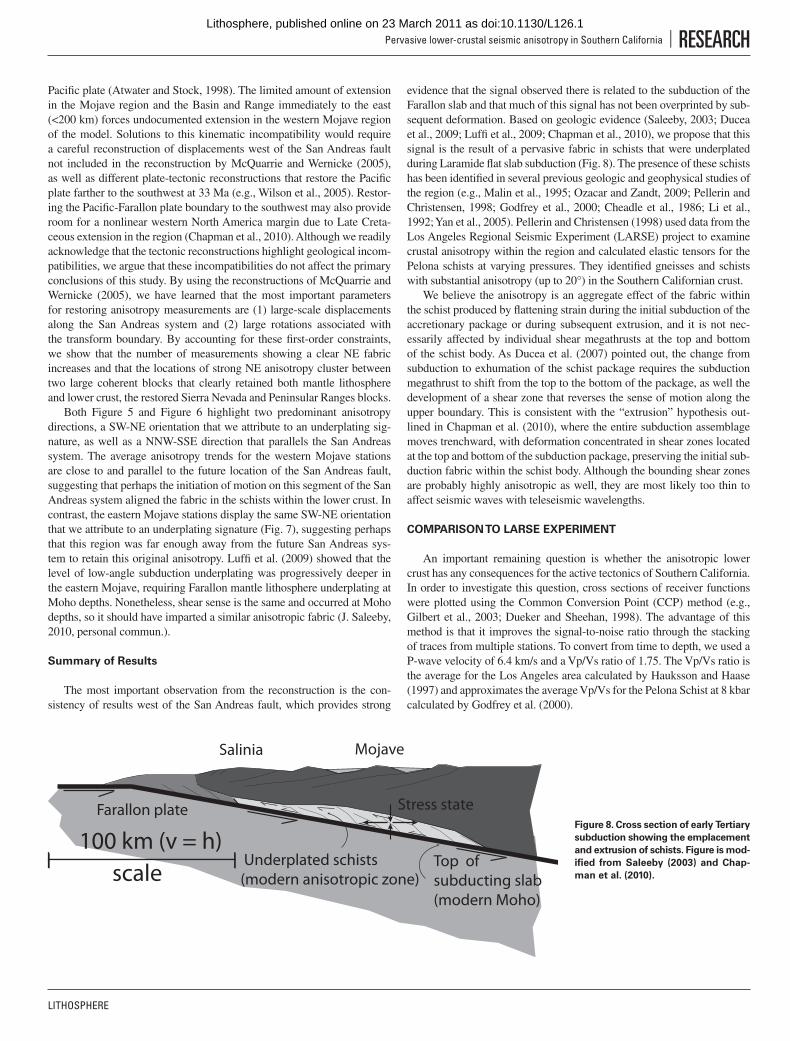
LITHOSPHERE

Pervasive lower-crustal seismic anisotropy in Southern California | RESEARCH

Pacifi c plate (Atwater and Stock, 1998). The limited amount of extension in the Mojave region and the Basin and Range immediately to the east (<200 km) forces undocumented extension in the western Mojave region of the model. Solutions to this kinematic incompatibility would require a careful reconstruction of displacements west of the San Andreas fault not included in the reconstruction by McQuarrie and Wernicke (2005), as well as different plate-tectonic reconstructions that restore the Pacifi c plate farther to the southwest at 33 Ma (e.g., Wilson et al., 2005). Restor-ing the Pacifi c-Farallon plate boundary to the southwest may also provide room for a nonlinear western North America margin due to Late Creta-ceous extension in the region (Chapman et al., 2010). Although we readily acknowledge that the tectonic reconstructions highlight geological incom-patibilities, we argue that these incompatibilities do not affect the primary conclusions of this study. By using the reconstructions of McQuarrie and Wernicke (2005), we have learned that the most important parameters for restoring anisotropy measurements are (1) large-scale displacements along the San Andreas system and (2) large rotations associated with the transform boundary. By accounting for these fi rst-order constraints, we show that the number of measurements showing a clear NE fabric increases and that the locations of strong NE anisotropy cluster between two large coherent blocks that clearly retained both mantle lithosphere and lower crust, the restored Sierra Nevada and Peninsular Ranges blocks.

Both Figure 5 and Figure 6 highlight two predominant anisotropy directions, a SW-NE orientation that we attribute to an underplating sig-nature, as well as a NNW-SSE direction that parallels the San Andreas system. The average anisotropy trends for the western Mojave stations are close to and parallel to the future location of the San Andreas fault, suggesting that perhaps the initiation of motion on this segment of the San Andreas system aligned the fabric in the schists within the lower crust. In contrast, the eastern Mojave stations display the same SW-NE orientation that we attribute to an underplating signature (Fig. 7), suggesting perhaps that this region was far enough away from the future San Andreas sys-tem to retain this original anisotropy. Luffi et al. (2009) showed that the level of low-angle subduction underplating was progressively deeper in the eastern Mojave, requiring Farallon mantle lithosphere underplating at Moho depths. Nonetheless, shear sense is the same and occurred at Moho depths, so it should have imparted a similar anisotropic fabric (J. Saleeby, 2010, personal commun.).

Summary of Results

The most important observation from the reconstruction is the con-sistency of results west of the San Andreas fault, which provides strong

evidence that the signal observed there is related to the subduction of the Farallon slab and that much of this signal has not been overprinted by sub-sequent deformation. Based on geologic evidence (Saleeby, 2003; Ducea et al., 2009; Luffi et al., 2009; Chapman et al., 2010), we propose that this signal is the result of a pervasive fabric in schists that were underplated during Laramide fl at slab subduction (Fig. 8). The presence of these schists has been identifi ed in several previous geologic and geophysical studies of the region (e.g., Malin et al., 1995; Ozacar and Zandt, 2009; Pellerin and Christensen, 1998; Godfrey et al., 2000; Cheadle et al., 1986; Li et al., 1992; Yan et al., 2005). Pellerin and Christensen (1998) used data from the Los Angeles Regional Seismic Experiment (LARSE) project to examine crustal anisotropy within the region and calculated elastic tensors for the Pelona schists at varying pressures. They identifi ed gneisses and schists with substantial anisotropy (up to 20°) in the Southern Californian crust.

We believe the anisotropy is an aggregate effect of the fabric within the schist produced by fl attening strain during the initial subduction of the accretionary package or during subsequent extrusion, and it is not nec-essarily affected by individual shear megathrusts at the top and bottom of the schist body. As Ducea et al. (2007) pointed out, the change from subduction to exhumation of the schist package requires the subduction megathrust to shift from the top to the bottom of the package, as well the development of a shear zone that reverses the sense of motion along the upper boundary. This is consistent with the “extrusion” hypothesis out-lined in Chapman et al. (2010), where the entire subduction assemblage moves trenchward, with deformation concentrated in shear zones located at the top and bottom of the subduction package, preserving the initial sub-duction fabric within the schist body. Although the bounding shear zones are probably highly anisotropic as well, they are most likely too thin to affect seismic waves with teleseismic wavelengths.

COMPARISON TO LARSE EXPERIMENT

An important remaining question is whether the anisotropic lower crust has any consequences for the active tectonics of Southern California. In order to investigate this question, cross sections of receiver functions were plotted using the Common Conversion Point (CCP) method (e.g., Gilbert et al., 2003; Dueker and Sheehan, 1998). The advantage of this method is that it improves the signal-to-noise ratio through the stacking of traces from multiple stations. To convert from time to depth, we used a P-wave velocity of 6.4 km/s and a Vp/Vs ratio of 1.75. The Vp/Vs ratio is the average for the Los Angeles area calculated by Hauksson and Haase (1997) and approximates the average Vp/Vs for the Pelona Schist at 8 kbar calculated by Godfrey et al. (2000).

scale

100 km (v = h)

Farallon plate

Underplated schists(modern anisotropic zone)

Stress state

Salinia Mojave

Top of subducting slab(modern Moho)

Figure 8. Cross section of early Tertiary

subduction showing the emplacement

and extrusion of schists. Figure is mod-

ifi ed from Saleeby (2003) and Chap-

man et al. (2010).

as doi:10.1130/L126.1Lithosphere, published online on 23 March 2011

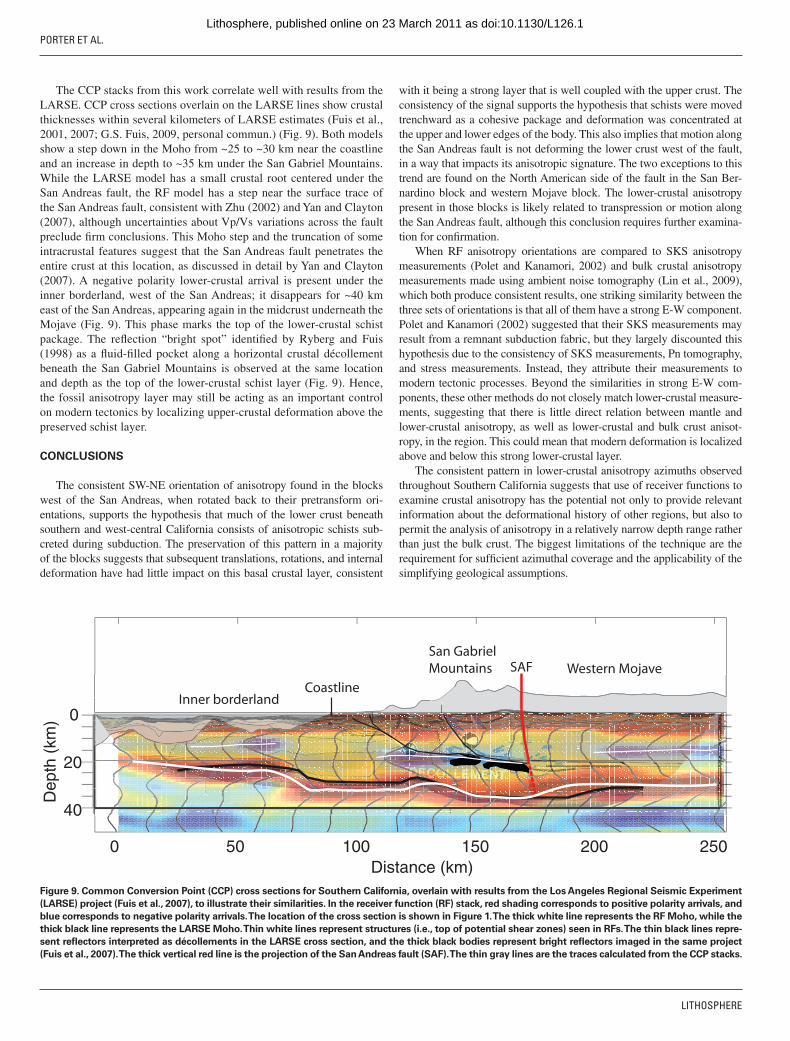
PORTER ET AL.

LITHOSPHERE

The CCP stacks from this work correlate well with results from the LARSE. CCP cross sections overlain on the LARSE lines show crustal thicknesses within several kilometers of LARSE estimates (Fuis et al., 2001, 2007; G.S. Fuis, 2009, personal commun.) (Fig. 9). Both models show a step down in the Moho from ~25 to ~30 km near the coastline and an increase in depth to ~35 km under the San Gabriel Mountains. While the LARSE model has a small crustal root centered under the San Andreas fault, the RF model has a step near the surface trace of the San Andreas fault, consistent with Zhu (2002) and Yan and Clayton (2007), although uncertainties about Vp/Vs variations across the fault preclude fi rm conclusions. This Moho step and the truncation of some intracrustal features suggest that the San Andreas fault penetrates the entire crust at this location, as discussed in detail by Yan and Clayton (2007). A negative polarity lower-crustal arrival is present under the inner borderland, west of the San Andreas; it disappears for ~40 km east of the San Andreas, appearing again in the midcrust underneath the Mojave (Fig. 9). This phase marks the top of the lower-crustal schist package. The refl ection “bright spot” identifi ed by Ryberg and Fuis (1998) as a fl uid-fi lled pocket along a horizontal crustal décollement beneath the San Gabriel Mountains is observed at the same location and depth as the top of the lower-crustal schist layer (Fig. 9). Hence, the fossil anisotropy layer may still be acting as an important control on modern tectonics by localizing upper-crustal deformation above the preserved schist layer.

CONCLUSIONS

The consistent SW-NE orientation of anisotropy found in the blocks west of the San Andreas, when rotated back to their pretransform ori-entations, supports the hypothesis that much of the lower crust beneath southern and west-central California consists of anisotropic schists sub-creted during subduction. The preservation of this pattern in a majority of the blocks suggests that subsequent translations, rotations, and internal deformation have had little impact on this basal crustal layer, consistent

with it being a strong layer that is well coupled with the upper crust. The consistency of the signal supports the hypothesis that schists were moved trenchward as a cohesive package and deformation was concentrated at the upper and lower edges of the body. This also implies that motion along the San Andreas fault is not deforming the lower crust west of the fault, in a way that impacts its anisotropic signature. The two exceptions to this trend are found on the North American side of the fault in the San Ber-nardino block and western Mojave block. The lower-crustal anisotropy present in those blocks is likely related to transpression or motion along the San Andreas fault, although this conclusion requires further examina-tion for confi rmation.

When RF anisotropy orientations are compared to SKS anisotropy measurements (Polet and Kanamori, 2002) and bulk crustal anisotropy measurements made using ambient noise tomography (Lin et al., 2009), which both produce consistent results, one striking similarity between the three sets of orientations is that all of them have a strong E-W component. Polet and Kanamori (2002) suggested that their SKS measurements may result from a remnant subduction fabric, but they largely discounted this hypothesis due to the consistency of SKS measurements, Pn tomography, and stress measurements. Instead, they attribute their measurements to modern tectonic processes. Beyond the similarities in strong E-W com-ponents, these other methods do not closely match lower-crustal measure-ments, suggesting that there is little direct relation between mantle and lower-crustal anisotropy, as well as lower-crustal and bulk crust anisot-ropy, in the region. This could mean that modern deformation is localized above and below this strong lower-crustal layer.

The consistent pattern in lower-crustal anisotropy azimuths observed throughout Southern California suggests that use of receiver functions to examine crustal anisotropy has the potential not only to provide relevant information about the deformational history of other regions, but also to permit the analysis of anisotropy in a relatively narrow depth range rather than just the bulk crust. The biggest limitations of the technique are the requirement for suffi cient azimuthal coverage and the applicability of the simplifying geological assumptions.

0 50 100 150 200 250

0

20

40

Dep

th (

km)

Distance (km)

SAFSan Gabriel

Mountains Western Mojave

Inner borderlandCoastline

´́́́́́́́́́́́́́́́́́́́́́́́́

Figure 9. Common Conversion Point (CCP) cross sections for Southern California, overlain with results from the Los Angeles Regional Seismic Experiment

(LARSE) project (Fuis et al., 2007), to illustrate their similarities. In the receiver function (RF) stack, red shading corresponds to positive polarity arrivals, and

blue corresponds to negative polarity arrivals. The location of the cross section is shown in Figure 1. The thick white line represents the RF Moho, while the

thick black line represents the LARSE Moho. Thin white lines represent structures (i.e., top of potential shear zones) seen in RFs. The thin black lines repre-

sent refl ectors interpreted as décollements in the LARSE cross section, and the thick black bodies represent bright refl ectors imaged in the same project

(Fuis et al., 2007). The thick vertical red line is the projection of the San Andreas fault (SAF). The thin gray lines are the traces calculated from the CCP stacks.

as doi:10.1130/L126.1Lithosphere, published online on 23 March 2011

LITHOSPHERE

Pervasive lower-crustal seismic anisotropy in Southern California | RESEARCH

APPENDIX A

Salinian Block

The Salinian block or Salinian “composite terrane” (Vedder et al., 1983) is bounded to the northeast by the San Andreas fault and to the south by the Sur-Nacimiento fault (Mattinson, 1978). The block has undergone ~315 km of northward transport since the mid-Miocene (Dickinson and Wernicke, 1997) and can be correlated structurally with rocks from the southern Sierra Nevada block (Dickinson and Butler, 1998; Ross, 1984). During the Laramide, the subduct-ing slab remained at a shallow depth beneath Salinia, reaching a depth of only 35 km, ~170 km inboard from the trench (Ducea et al., 2009). This removed lower-crustal material and underplated the lower crust with trench sediments. The lower crust within the Salinian block is believed to be composed of the Sierra de Salinas schist, which is correlative to the Pelona, Orocopia, and Rand schists that underlie much of Southern California and western Arizona (Ducea et al., 2009). Stations MPP, PHL, and PKD are located within the Salinian block.

San Gabriel Block

The San Gabriel block lies between the San Bernardino and Western Trans-verse Ranges blocks and contains the stations BFS, CHF, MWC, OSI, VCS, and most likely DEC (in the reconstruction, this station lies within the Western Transverse Ranges). The block is composed of Mesozoic and older igneous and metamorphic rocks thrust over the Pelona Schist (Jacobson, 1983; Jacobson et al., 1996). While this block has not experienced the rotation of the Western Trans-verse Ranges block, it has moved 270 km northward since the mid-Miocene and has most likely experienced the same ~53–60 km shortening since ca. 3 Ma as calculated for the Western Transverse Ranges block directly to the west (Namson and Davis, 1988; McQuarrie and Wernicke, 2005).

Western Transverse Ranges

The Transverse Ranges consist of E-W–running mountain ranges uplifted due to transpression within the restraining bend in the San Andreas fault (Ehlig, 1981; Wright, 1991). Based on the reconstruction of McQuarrie and Wernicke (2005), we divided the Transverse Ranges into three separate crustal blocks for our interpreta-tion: the Western Transverse Ranges block, the San Bernardino block, and the Cen-tral Transverse Ranges or San Gabriel block. The Transverse Ranges also consist of the Eastern Transverse Ranges block, which is not included in our interpretations.

The Western Transverse Ranges block consists of the region west of the San Gabriel Mountains and includes the southern part of the Santa Ynez Mountain (Fig. 1); stations DJJ, TOV, PAS, and PASC lie within this block. During the early Miocene, this block was located on the western side of the Baja block; since that time, it has moved ~260–270 km north and rotated ~90°–117° clockwise (Hornafi us et al., 1986; Luyendyk et al., 1980; Luyendyk 1991). Crustal shortening of ~53–60 km along a midcrustal detachment is believed to have occurred within this block since 3 Ma, resulting in high topography and a deformed crust (Namson and Davis, 1988).

Continental Borderland

Beginning in the early Miocene, the continental borderland, located off the coast of California (Fig. 1), experienced extension comparable in both style and magni-tude to that seen in the Basin and Range Province of the southwestern United States (Bohannon and Geist, 1998). The province is separated into the inner and outer bor-derland (Crouch and Suppe, 1993); we concerned ourselves primarily with the inner borderland, because all the seismic stations used in this work fall within this area. Basement rocks in the inner borderland consist primarily of Mesozoic-age blueschists and greenschists from the Catalina terrane (Howell and Vedder, 1981; Wright, 1991). The topography of the inner borderland consists of several NW-trending submerged basins and ridges that formed during the mid-Miocene, in the wake of clockwise rotation of the Western Transverse Ranges (Howell and Vedder, 1981; Wright, 1991; Crouch and Suppe, 1993). Prior to rotation of the Transverse Ranges and the accom-panying extension, in the borderlands, McQuarrie and Wernicke (2005) proposed that the continental borderland behaved as part of the Baja block. Deformation within the continental borderland occurred along NW-striking oblique normal faults (Wright, 1991). The stations CIA, CIU, SNCC, RPV, and FMP lie within the block.

Peninsular Ranges

In reconstructions of western North America, the Peninsular Ranges are con-sidered part of the Baja block (McQuarrie and Wernicke, 2005), which has moved

~276 km northward from 6 Ma to present (Oskin et al., 2001; Oskin and Stock, 2003). Stations CRY, KNW, RDM, SND, TRO, WMC, and YAQ are located within the Baja block. The Peninsular Ranges are a large batholith that extends 1000 km from Southern California to the tip of the Baja Peninsula (Silver and Chappell, 1988). For this study, we focus on the San Jacinto Mountains, located at the north-ern end of the range. The mountains are bifurcated by the San Jacinto fault, a right-lateral splay of the San Andreas fault. It has been argued that this fault formed at a compositional boundary between older, more mafi c rocks to the west and younger, more felsic rocks to the east (Magistrale and Sanders, 1995), and that this bound-ary is related to structures that predate the batholith (Langenheim et al., 2004). A 10°W-dipping Moho has been identifi ed across this boundary in the northern Peninsular Ranges (Lewis et al., 2000).

Mojave Block

The Mojave block is the part of the Mojave Desert that is bounded to the south-west by the San Andreas fault, to the north by the Garlock fault, and to the east by the southern edge of the Death Valley fault zone (Glazner et al., 2002). From ca. 24 Ma to present, the Mojave block has experienced two phases of deforma-tion, early Miocene extension and volcanism, and late Tertiary right-lateral shear (e.g., McQuarrie and Wernicke, 2005). Early Miocene extension in the Mojave was focused in the central Mojave metamorphic core complex (Glazner et al., 1989; Walker et al., 1990; Martin et al., 1993; Fletcher et al., 1995; Glazner et al., 2002), which accommodated 40–50 km of E-W extension between 24 and 18 Ma (Glazner et al., 1989; Martin et al., 1993; Ingersoll et al., 1996). Post-extension deforma-tion largely occurred along strike-slip faults that may have accommodated up to 100 km of shear since ca. 12 Ma (McQuarrie and Wernicke, 2005). The Mojave block contains the Eastern California shear zone, a 100-km-wide system of right-lateral faults formed due to the relative motion between the North American and Pacifi c plates (e.g., Savage et al., 1990, 2001). Geodetically, the Eastern California shear zone accommodates ~25% of the relative plate motion between the North America and Pacifi c plates (Sauber et al., 1994; Miller et al., 2001; McClusky et al., 2001). Based on paleomagnetic data, it is argued that the northeastern Mojave has experienced up to 60° of clockwise rotation (Shermer et al., 1996; Luyendyk, 1991; Luyendyk et al., 1980). For this project, we divided the Mojave into eastern and western components separated by the Eastern California shear zone. Stations EDW2, LKL, and VTV lie in the western Mojave, and stations HEC, GSC, JVA, RRX, and TUQ lie in the east.

San Bernardino Block

The San Bernardino block consists primarily of the San Bernardino Moun-tains, and it contains the stations SBPX, BBR, as well as station SVD, which lies directly on the San Andreas fault but falls just west of the fault in the reconstruction of McQuarrie and Wernicke (2005). The geology of the San Bernardino block is strongly tied to the southern Mojave, with basement rocks in the San Bernardino block having direct correlatives to the immediately adjacent Mojave basement near Victorville (Stewart and Poole, 1974; Miller, 1981). Likewise, the displace-ment history of the San Bernardino block is proposed to be similar to the southern Mojave. The block moved to the northwest synchronous with right-lateral shear in the Mojave and rotation of the Eastern Transverse Ranges (e.g., McQuarrie and Wernicke, 2005) and has experienced an unknown amount of post-Miocene rota-tion (Luyendyk, 1991). The block is composed largely of Proterozoic and Mesozoic igneous and metamorphic rocks, overlain by Tertiary deposits (Langenheim and Powell, 2009). The Orocopia schist is present beneath much of the San Bernardino block (Powell, 1981).

Eastern Transverse Ranges Block

The Eastern Transverse Ranges block lies to the southeast of the San Ber-nardino block and contains the Little San Bernardino Mountains and the land between the Pinto Mountain fault and the San Andreas fault. Stations BLA and BEL lie within the block. The tectonic block has been rotated clockwise ~41° in the past 10 m.y. Inversions run on the two stations located within the block do not produce consistent azimuths of anisotropy, and therefore they were not included in our interpretation for the region.

APPENDIX B

The value of η defi nes the curvature of the velocity “ellipsoid” between the Vp-fast and Vp-slow axes. Using the nomenclature of Love (1927, cited in Babuska and Cara, 1991), the elastic tensor for hexagonal anisotropy is:

as doi:10.1130/L126.1Lithosphere, published online on 23 March 2011

PORTER ET AL.

LITHOSPHERE

C

A A N FA N A F

F F CL

LN

ij =

−−

2 0 0 02 0 0 0

0 0 00 0 0 0 00 0 0 0 00 0 0 0 0

, (1)

where

A VP= ρ 902

°, (2)

C VP= ρ 02

°, (3)

N VSH= ρ 902

°, (4)

L VSV= ρ 02

°, (5)

F L V V A C L A L C LP P= − + ( ) − ( ) + +( ) + +( ) +( )⎡ 4 2 2245

445

2ρ ρ° °⎣⎣ ⎤⎦ , (6)

(Okaya and Christensen, 2002), and the parameter η is defi ned as:

η =−( )F

A L2, (7)

(Sherrington et al., 2004).Levin and Park (1997) used the parameters a, b, c, d, and e to defi ne anisotropy,

where:

ρ ξ ξV a b cp2 2 4= + ( ) + ( )cos cos , (8)

ρ ξV d eS2 2= + ( )cos . (9)

The variable ξ is the angle between the wave propagation and the axis of sym-metry. The parameter a corresponds to average P velocity, b to the azimuthal varia-tion in P velocity, c to anisotropy ellipsoid variations away from a true ellipsoid, d to the average S velocity, and e to the azimuthal variations in S velocity. For the anisotropy inversion, the velocity ellipsoid was assumed to be a true ellipsoid (c = 0), as has been assumed in several previous studies (Ozacar and Zandt, 2009; Sherrington et al., 2004; Levin and Park, 1997). The purpose of this assumption is to improve the inversion to calculate more reasonable anisotropy values. If η is kept independent of percent anisotropy, it is possible to produce a signifi cant anisotropic signal with 0% anisotropy by deforming the velocity ellipsoid so that Vp-45° is equivalent to Vp-max. In assuming a pure ellipsoid, η becomes a function of percent anisotropy. Previous work calculating elastic tensors for the schists in the region has assumed hexagonal anisotropy (Godfrey et al., 2000). Further work is required to determine if signifi cant perturbations from an ellipse are detectable with this technique. Relating η to percent anisotropy also allows us to approximate η while reducing the number of free parameters in the inversion, which in turn increases its stability.

ACKNOWLEDGMENTS

We thank Mihai Ducea, Brad Hacker, and Arda Ozacar, who contributed to our understanding of regional geology and crustal anisotropy, and Vladim Levin, who reviewed an early version of this work. Arda Ozacar got us started looking at the Southern California data. We thank Andrew Frederiksen for sharing the original rasyum code, Kiriaki Xiluri and Steve Sorenson for help modifying it, and Andy Frassetto, Josh Calkins, and Hersh Gilbert for help with the Common Conversion Point codes. Chris-tine Gans and Arda Ozacar provided useful feedback on an early version of the manuscript. We thank Jason Saleeby for his detailed review regard-

ing the geology and tectonics of Southern California. His comments and suggested changes were instrumental in our revisions, but any remain-ing misinterpretations are strictly the responsibility of the authors. This work was funded by a grant from Southern California Earthquake Center and National Science Foundation (NSF) EAR Earthscope Program award 0745588. Figures 1 and 6 were made using Generic Mapping Tools (Wes-sel and Smith, 1995).

REFERENCES CITED

Alexandrov, K.S., and Ryzhova, T.V., 1961, Elastic properties of rock-forming minerals: II. Lay-ered silicates: Bulletin of the Academy of Sciences of the U.S.S.R. Geophysics Series, v. 12, p. 1799–1804.

Atwater, T., 1989, Plate tectonic history of the northeast Pacifi c and western North America, in Winterer, E.L., Hussong, D.M., and Decker, R.W., eds., The Eastern Pacifi c Ocean and Hawaii: Boulder, Colorado, Geological Society of America, The Geology of North America, v. N, p. 21–72.

Atwater, T., and Stock, J., 1998, Pacifi c–North America plate tectonics of the Neogene south-western United States: An update: International Geology Review, v. 40, p. 375–402, doi:10.1080/00206819809465216.

Babuska, V., and Cara, M., 1991, Seismic Anisotropy in the Earth: Boston, Kluwer Academic Publishers, 232 p.

Barruol, G., and Kern, H., 1996, Seismic anisotropy and shear wave splitting in the lower crustal/upper mantle transition (Ivrea zone): Experimental and calculated data: Physics of the Earth and Planetary Interiors, v. 95, p. 175–194, doi:10.1016/0031-9201(95)03124-3.

Bohannon, R.G., and Geist, E.L., 1998, Upper crustal structure and Neogene tectonic devel-opment of the California continental borderland: Geological Society of America Bulle-tin, v. 110, p. 779–800, doi:10.1130/0016-7606(1998)110<0779:UCSANT>2.3.CO;2.

Chapman, A.D., Kidder, S., Saleeby, J.B., and Ducea, M.N., 2010, Role of extrusion of the Rand and Sierra de Salinas Schists in Late Cretaceous extension and rotation of the southern Sierra Nevada and vicinity: Tectonics, v. 29, TC5006, doi:10.1029/2009TC002597.

Cheadle, M.J., Czuchra, B.L., Byrne, T., Ando, C.J., Oliver, J.E., Brown, L.D., Kaufman, S., Malin, P.E., and Phinney, R.A., 1986, The deep crustal structure of the Mojave Des-ert, California, from COCORP seismic refl ection data: Tectonics, v. 5, p. 293–320, doi:10.1029/TC005i002p00293.

Crouch, J.K., and Suppe, J., 1993, Late Cenozoic tectonic evolution of the Los Angeles Basin and inner California borderland: A model for core complex–like crustal exten-sion: Geological Society of America Bulletin, v. 105, p. 1415–1434, doi:10.1130/0016-7606(1993)105<1415:LCTEOT>2.3.CO;2.

Dickinson, W.R., 1996, Kinematics of Transrotational Tectonism in the California Transverse Ranges and Its Contribution to Cumulative Slip along the San Andreas Transform Fault System: Geological Society of America Special Paper 305, 46 p.

Dickinson, W.R., and Butler, R.F., 1998, Coastal and Baja California paleomagnetism recon-sidered: Geological Society of America Bulletin, v. 110, p. 1268–1280, doi:10.1130/0016-7606(1998)110<1268:CABCPR>2.3.CO;2.

Dickinson, W.R., and Wernicke, B.P., 1997, Reconciliation of San Andreas slip discrepancy by a combination of interior Basin and Range extension and transrotation near the coast: Geology, v. 25, p. 663–665, doi:10.1130/0091-7613(1997)025<0663:ROSASD>2.3.CO;2.

Dokka, R.K., and Travis, C.J., 1990, Late Cenozoic strike-slip faulting in the Mojave Desert, California: Tectonics, v. 9, p. 311–340, doi:10.1029/TC009i002p00311.

Ducea, M.N., Kidder, S., and Chesley, J.T., 2007, A geologic window into a subduction mega-thrust: Eos (Transactions, American Geophysical Union), v. 88, p. 277, doi:10.1029/2007EO270001.

Ducea, M.N., Kidder, S., Chesley, J.T., and Saleeby, J.B., 2009, Tectonic underplating of trench sediments beneath magmatic arcs: The central California example: International Geology Review, v. 51, p. 1–26, doi:10.1080/00206810802602767.

Dueker, K.G., and Sheehan, A.F., 1998, Mantle discontinuity structure beneath the Colorado Rocky Mountains and High Plains: Journal of Geophysical Research, v. 103, p. 7153–7169, doi:10.1029/97JB03509.

Ehlig, P.L., 1981, Origin and tectonic history of the basement terrane of the San Gabriel Mountains, central Transverse Ranges, in Ernst, W.G., ed., The Geotectonic Develop-ment of California: Englewood Cliffs, New Jersey, Prentice-Hall, Inc., p. 253–283.

Fletcher, J.M., Bartley, J.M., Martin, M.W., Glazner, A.F., and Walker, J.D., 1995, Large-mag-nitude continental extension: An example from the central Mojave metamorphic core complex: Geological Society of America Bulletin, v. 107, p. 1468–1483, doi:10.1130/0016-7606(1995)107<1468:LMCEAE>2.3.CO;2.

Frederiksen, A.W., and Bostock, M.G., 2000, Modelling teleseismic waves in dipping aniso-tropic structures: Geophysical Journal International, v. 141, p. 401–412, doi:10.1046/j.1365-246x.2000.00090.x.

Frederiksen, A.W., Folsom, H., and Zandt, G., 2003, Neighbourhood inversion of teleseismic Ps conversions for anisotropy and layer dip: Geophysical Journal International, v. 155, p. 200–212, doi:10.1046/j.1365-246X.2003.02043.x.

Fuis, G.S., Ryberg, T., Godfrey, N.J., Okaya, D.A., and Murphy, J.M., 2001, Crustal structure and tectonics from the Los Angeles basin to the Mojave Desert, Southern California: Geology, v. 29, p. 15–18, doi:10.1130/0091-7613(2001)029<0015:CSATFT>2.0.CO;2.

Fuis, G.S., Kohler, M.D., Scherwath, M., ten Brink, U., Van Avendonk, H.J.A., and Murphy, J.M., 2007, A comparison between the transpressional plate boundaries of the South Island, New Zealand, and Southern California, USA: The Alpine and San Andreas fault systems, in Okaya, D., Stern, T., and Davey, F., eds., A Continental Plate Boundary:

as doi:10.1130/L126.1Lithosphere, published online on 23 March 2011

LITHOSPHERE

Pervasive lower-crustal seismic anisotropy in Southern California | RESEARCH

Tectonics at South Island, New Zealand: American Geophysical Union Geophysical Monograph 175, p. 307–327.

Gilbert, H.J., Sheehan, A.F., Dueker, K.G., and Molnar, P., 2003, Receiver functions in the western United States, with implications for upper mantle structure and dynamics: Journal of Geophysical Research, v. 108, 2229, 19 p., doi:10.1029/2001JB001194.

Glazner, A.F., Bartley, J.M., and Walker, J.D., 1989, Magnitude and signifi cance of Miocene crustal extension in the central Mojave Desert, California: Geology, v. 17, p. 50–53, doi:10.1130/0091-7613(1989)017<0050:MASOMC>2.3.CO;2.

Glazner, A.F., Walker, J.D., Bartley, J.M., and Fletcher, J.M., 2002, Cenozoic evolution of the Mojave block of Southern California, in Glazner A.F., Walker, J.D., and Bartley, J.M., eds., Geologic Evolution of the Mojave Desert and Southwestern Basin and Range: Geological Society of America Memoir 195, p. 19–41, doi:10.1130/0-8137-1195-9.19.

Godfrey, N.J., Christensen, N.I., and Okaya, D.A., 2000, Anisotropy of schists: Contribution of crustal anisotropy to active source seismic experiments and shear wave splitting observa-tions: Journal of Geophysical Research, v. 105, p. 27,991–28,007, doi:10.1029/2000JB900286.

Godfrey, N.J., Fuis, G.S., Langenheim, V., Okaya, D.A., and Brocher, T.M., 2002, Lower crustal deformation beneath the central Transverse Ranges, Southern California: Results from the Los Angeles region seismic experiment: Journal of Geophysical Research, v. 107, 2144, doi:10.1029/2001JB000354.

Graham, S.A., Stanley, R.G., Bent, J.V., and Carter, J.R., 1989, Oligocene and Miocene paleo-geography of central California and displacement along the San Andreas fault: Geologi-cal Society of America Bulletin, v. 101, p. 711–730, doi:10.1130/0016-7606(1989)101<0711:OAMPOC>2.3.CO;2.

Grove, M., and Bebout, G.E., 1995, Cretaceous tectonic evolution of coastal Southern California: insights from the Catalina Schist: Tectonics, v. 14, p. 1290–1308, doi:10.1029/95TC01931.

Grove, M., Jacobson, C.E., Barth, A.P., and Vucic, A., 2003, Temporal and spatial trends of Late Cretaceous–early Tertiary underplating of Pelona and related schist beneath Southern California and southwestern Arizona, in Johnson, S.E., Paterson, S.R., Fletcher, J.M., Girty, G.H., Kimbrough, D.L., and Martin-Barajas, A., eds., Tectonic Evolution of North-western Mexico and the Southwestern USA: Geological Society of America Special Paper 374, p. 381–406, doi:10.1130/0-8137-2374-4.381.

Hauksson, E., and Haase, J.S., 1997, Three-dimensional Vp and Vp/Vs velocity models of the Los Angeles basin and central Transverse Ranges, California: Journal of Geophysical Research, v. 102, p. 5423–5453, doi:10.1029/96JB03219.

Hornafi us, J.S., Luyendyk, B.P., Terres, R.R., and Kamerling, M.J., 1986, Timing and extent of Neogene tectonic rotation in the Western Transverse Ranges, California: Geological Society of America Bulletin, v. 97, p. 1476–1487, doi:10.1130/0016-7606(1986)97<1476:TAEONT>2.0.CO;2.

Howard, K.A., and Miller, D.M., 1992, Late Cenozoic faulting at the boundary between the Mojave and Sonoran blocks; Bristol Lake area, California, in Richard, S.M., ed., Deformation Associ-ated with the Neogene, Eastern California Shear Zone, Southeastern California and South-western Arizona; proceedings: Redlands, California, San Bernardino County Museum Asso-ciation, San Bernardino County Museum Association Special Publication 92-1, p. 37–47.

Howell, D.G., and Vedder, J., 1981, Structural implications of stratigraphic discontinuities across the Southern California borderland, in Ernst, W.C., ed., The Geotectonic Develop-ment of California, Volume 1: Englewood Cliffs, New Jersey, Prentice-Hall, p. 535–558.

Ingersoll, R.V., Devaney, K.A., Geslin, J.K., Cavazza, W., Diamond, D.S., Heins, W.A., Jagiello, K.J., Marsaglia, K.M., Paylor, E.D., II, and Short, P.F., 1996, The Mud Hills, Mojave Desert, California: Structure, stratigraphy, and sedimentology of a rapidly extended terrane, in Beratan, K.K., ed., Reconstructing the History of Basin and Range Extension Using Sedimentology and Stratigraphy: Geological Society of America Special Paper 303, p. 61–84, doi:10.1130/0-8137-2303-5.61.

Jacobson, C.E., 1983, Structural geology of the Pelona Schist and Vincent thrust, San Gabriel Mountains, California: Geological Society of America Bulletin, v. 94, p. 753–767, doi:10.1130/0016-7606(1983)94<753:SGOTPS>2.0.CO;2.

Jacobson, C.E., Oyarzabal, F.R., and Haxel, G.B., 1996, Subduction and exhumation of the Pelona-Orocopia-Rand schists, Southern California: Geology, v. 24, p. 547–550, doi:10.1130/0091-7613(1996)024<0547:SAEOTP>2.3.CO;2.

Kidder, S., and Ducea, M.N., 2006, High temperatures and inverted metamorphism in the schist of Sierra de Salinas, California: Earth and Planetary Science Letters, v. 241, p. 422–437, doi:10.1016/j.epsl.2005.11.037.

Kohlstedt, D.L., and Holtzman, B.K., 2009, Shearing melt out of the Earth: An experimentalist’s perspective on the infl uence of deformation on melt extraction: Annual Review of Earth and Planetary Sciences, v. 37, p. 561–593, doi:10.1146/annurev.earth.031208.100104.

Langenheim, V.E., and Powell, R.E., 2009, Basin geometry and cumulative offsets in the East-ern Transverse Ranges, Southern California: Implications for transrotational deformation along the San Andreas fault system: Geosphere, v. 5, p. 1–22, doi:10.1130/GES00177.1.

Langenheim, V.E., Jachens, R.C., Morton, D.M., Kistler, R.W., and Matti, J.C., 2004, Geophysi-cal and isotopic mapping of preexisting crustal structures that infl uenced the location and development of the San Jacinto fault zone, Southern California: Geological Society of America Bulletin, v. 116, p. 1143–1157, doi:10.1130/B25277.1.

Langston, C., 1979, Structure under Mt. Ranier, Washington, inferred from teleseismic body waves: Journal of Geophysical Research, v. 84, p. 4749–4762, doi:10.1029/JB084iB09p04749.

Levin, V., and Park, J., 1997, P-SH conversions in a fl at-layered medium with anisotropy of arbitrary orientation: Geophysical Journal International, v. 131, p. 253–266, doi:10.1111/j.1365-246X.1997.tb01220.x.

Levin, V., and Park, J., 1998, P-SH conversions in layered media with hexagonally symmet-ric anisotropy: A cookbook: Pure and Applied Geophysics, v. 151, 29 p., doi:10.1007/s000240050136.

Lewis, J.L., Day, S.M., Magistrale, H., Eakins, J., and Vernon, F., 2000, Regional crustal thick-ness variations of the Peninsular Ranges, Southern California: Geology, v. 28, p. 303–306, doi:10.1130/0091-7613(2000)28<303:RCTVOT>2.0.CO;2.

Li, Y.-G., Henyey, T.L., and Silver, L.T., 1992, Aspects of the crustal structure of the western Mojave Desert, California, from seismic refl ection and gravity data: Journal of Geo-physical Research, v. 97, no. B6, p. 8805–8816, doi:10.1029/91JB02119.

Ligorria, J.P., and Ammon, C.J., 1999, Iterative deconvolution and receiver-function estima-tion: Bulletin of the Seismological Society of America, v. 89, p. 6.

Lin, F.C., Ritzwoller, M.H., and Snieder, R., 2009, Eikonal tomography: Surface wave tomog-raphy by phase front tracking across a regional broad-band seismic array: Geophysical Journal International, v. 177, p. 1091–1110, doi:10.1111/j.1365-246X.2009.04105.x.

Luffi , P., Saleeby, J.B., Lee, C.T.A., and Ducea, M.N., 2009, Lithospheric mantle duplex beneath the central Mojave Desert revealed by xenoliths from Dish Hill, California: Journal of Geophysical Research, v. 114, B03202, doi:10.1029/2008JB005906.

Luyendyk, B.P., 1991, A model for Neogene crustal rotations, transtension, and transpression in Southern California: Geological Society of America Bulletin, v. 103, p. 1528–1536, doi:10.1130/0016-7606(1991)103<1528:AMFNCR>2.3.CO;2.

Luyendyk, B.P., Kamerling, M.J., and Terres, R., 1980, Geometric model for Neogene crustal rotations in Southern California: Geological Society of America Bulletin, v. 91, p. 211–217, doi:10.1130/0016-7606(1980)91<211:GMFNCR>2.0.CO;2.

Magistrale, H., and Sanders, C., 1995, P-wave image of the Peninsular Ranges Batholith, South-ern California: Geophysical Research Letters, v. 22, p. 2549–2552, doi:10.1029/95GL02241.

Malin, P.E., Goodman, E.D., Henyey, T.L., Li, Y.G., Okaya, D.A., and Saleeby, J.B., 1995, Sig-nifi cance of seismic refl ections beneath a tilted exposure of deep continental crust, Tehachapi Mountains, California: Journal of Geophysical Research, v. 100, p. 2069–2087, doi:10.1029/94JB02127.

Martin, M.W., Glazner, A.F., Walker, J.D., and Schermer, E.R., 1993, Evidence for right-lateral transfer faulting accommodating en echelon Miocene extension, Mojave Desert, Califor-nia: Geology, v. 21, p. 355–358, doi:10.1130/0091-7613(1993)021<0355:EFRLTF>2.3.CO;2.

Matthews, V., III, 1976, Correlation of Pinnacles and Neenach volcanic formations and their bearing on the San Andreas problem: American Association of Petroleum Geologists Bulletin, v. 51, p. 2128–2141.

Mattinson, J.M., 1978, Age, origin, and thermal histories of some plutonic rocks from the Salinian block of California: Contributions to Mineralogy and Petrology, v. 67, p. 233–245, doi:10.1007/BF00381451.

McClusky, S.C., Bjornstad, S.C., Hager, B.H., King, R.W., Meade, B.J., Miller, M.M., Monas-tero, F.C., and Souter, B.J., 2001, Present day kinematics of the Eastern California shear zone from a geodetically constrained block model: Geophysical Research Letters, v. 28, p. 3369–3372, doi:10.1029/2001GL013091.

McQuarrie, N., and Oskin, M., 2010, Palinspastic restoration of NAVDat and implications for the origin of magmatism in southwestern North America: Journal of Geophysical Research, v. 115, B10401, doi:10.1029/2009JB006435.

McQuarrie, N., and Wernicke, B.P., 2005, An animated tectonic reconstruction of southwest-ern North America since 36 Ma: Geosphere, v. 1, p. 147–172.

Miller, E.L., 1981, Geology of the Victorville region, California: Geological Society of America Bulletin, v. 92, Part II, p. 554–608.

Miller, M.M., Johnson, D.J., Dixon, T.H., and Dokka, R.K., 2001, Refi ned kinematics of the Eastern California shear zone from GPS observations, 1993–1998: Journal of Geophysi-cal Research, v. 106, p. 2245–2263, doi:10.1029/2000JB900328.

Muehlberger, W.R., 1996, Tectonic Map of North America: Tulsa, Oklahoma, American Asso-ciation of Petroleum Geologists, 2 sheets, scale 1:5,000,000.

Namson, J., and Davis, T., 1988, Structural transect of the Western Transverse Ranges Cali-fornia: Implications for lithospheric kinematics and seismic risk evaluation: Geology, v. 16, p. 675–679, doi:10.1130/0091-7613(1988)016<0675:STOTWT>2.3.CO;2.

Nicholson, C., Sorlien, C.C., Atwater, T., Crowell, J.C., and Luyendyk, B.P., 1994, Microplate capture, rotation of the Western Transverse Ranges, and initiation of the San Andreas transform as a low-angle fault system: Geology, v. 22, p. 491–495, doi:10.1130/0091-7613(1994)022<0491:MCROTW>2.3.CO;2.

Okaya, D.A., and Christensen, N.I., 2002, Anisotropic effects of non-axial seismic wave prop-agation in foliated crustal rocks: Geophysical Research Letters, v. 29, 1507, doi:10.1029/2001GL014285.

Okaya, D.A., and McEvilly, T.V., 2003, Elastic wave propagation in anisotropic crustal material possessing arbitrary internal tilt: Geophysical Journal International, v. 153, p. 344–358, doi:10.1046/j.1365-246X.2003.01896.x.

Oskin, M., and Stock, J., 2003, Pacifi c–North America plate motion and opening of the Upper Delfín basin, northern Gulf of California, Mexico: Geological Society of America Bul-letin, v. 115, p. 1173–1190, doi:10.1130/B25154.1.

Oskin, M., Stock, J., and Martin-Barajas, A., 2001, Rapid localization of Pacifi c–North America plate motion in the Gulf of California: Geology, v. 29, p. 459–462, doi:10.1130/0091-7613(2001)029<0459:RLOPNA>2.0.CO;2.

Ozacar, A.A., and Zandt, G., 2004, Crustal seismic anisotropy in central Tibet: Implications for deformational style and fl ow in the crust: Geophysical Research Letters, v. 31, L23601, doi:10.1029/2004GL021096.

Ozacar, A.A., and Zandt, G., 2009, Crustal structure and seismic anisotropy near the San Andreas fault at Parkfi eld, California: Geophysical Journal International, v. 178, p. 1098–1104, doi:10.1111/j.1365-246X.2009.04198.x.

Pellerin, C., and Christensen, N.I., 1998, Interpretation of crustal seismic velocities in the San Gabriel–Mojave region, Southern California: Tectonophysics, v. 286, p. 253–271, doi:10.1016/S0040-1951(97)00269-2.

Peng, Z., and Humphreys, E.D., 1997, Moho dip and crustal anisotropy in northwestern Nevada from teleseismic receiver functions: Bulletin of the Seismological Society of America, v. 87, p. 745–754.

Polet, J., and Kanamori, H., 2002, Anisotropy beneath California: Shear wave splitting mea-surements using a dense broadband array: Geophysical Journal International, v. 149, p. 313–327, doi:10.1046/j.1365-246X.2002.01630.x.

as doi:10.1130/L126.1Lithosphere, published online on 23 March 2011

PORTER ET AL.

LITHOSPHERE

Powell, R.E., 1981, Geology of the Crystalline Basement Complex, Eastern Transverse Ranges, Southern California: Constraints on Regional Tectonic Interpretation [Ph.D. thesis]: Pasadena, California Institute of Technology, 441 p.

Ross, D.C., 1984, Possible Correlations of Basement Rocks across the San Andreas, San Gre-gorio–Hosgri, and Rinconada–Reliz–King City faults, California: U.S. Geological Survey Professional Paper 1317, 37 p.

Ryberg, T., and Fuis, G.S., 1998, The San Gabriel Mountains bright refl ective zone: Possible evidence of young mid-crustal thrust faulting in Southern California: Tectonophysics, v. 286, p. 31–46, doi:10.1016/S0040-1951(97)00253-9.

Saleeby, J., 2003, Segmentation of the Laramide slab—Evidence from the southern Sierra Nevada region: Geological Society of America Bulletin, v. 115, p. 655–668, doi:10.1130/0016-7606(2003)115<0655:SOTLSF>2.0.CO;2.

Sambridge, M., 1999, Geophysical inversion with a neighbourhood algorithm: I. Searching a parameter space: Geophysical Journal International, v. 138, p. 479–494, doi:10.1046/j.1365-246X.1999.00876.x.

Sauber, J., Thatcher, W., Solomon, S.C., and Lisowski, M., 1994, Geodetic slip rate for the Eastern California shear zone and the recurrence time of Mojave Desert earthquakes: Nature, v. 367, p. 264–266, doi:10.1038/367264a0.

Savage, J.C., Lisowski, M., and Prescott, W.H., 1990, An apparent shear zone trending north-northwest across the Mojave Desert into Owens Valley, eastern California: Geophysical Research Letters, v. 17, p. 2113–2116, doi:10.1029/GL017i012p02113.

Savage, J.C., Gan, W., and Svarc, J.L., 2001, Strain accumulation and rotation in the Eastern California shear zone: Journal of Geophysical Research, v. 106, p. 21,995–22,007.

Savage, M.K., 1998, Lower crustal anisotropy or dipping boundaries? Effects on receiver functions and a case study in New Zealand: Journal of Geophysical Research, v. 103, p. 15,069–15,087, doi:10.1029/98JB00795.

Schermer, E.R., Luyendyk, B.P., and Cisowski, S., 1996, Late Cenozoic structure and tectonics of the northern Mojave Desert: Tectonics, v. 15, p. 905–932.

Sherrington, H.F., Zandt, G., and Frederiksen, A., 2004, Crustal fabric in the Tibetan Plateau based on waveform inversions for seismic anisotropy parameters: Journal of Geo-physical Research, v. 109, B02312, doi:10.1029/2002JB002345.

Silver, L.T., and Chappell, B.W., 1988, The Peninsular Ranges Batholith: An insight into the evolution of the Cordilleran batholiths of southwestern North America: Transactions of the Royal Society of Edinburgh, Earth Sciences, v. 79, p. 105–121.

Stewart, J.H., and Poole, F.G., 1974, Lower Paleozoic and uppermost Precambrian Cordille-ran miogeocline, Great Basin, western United States, in Dickinson, W.R., ed., Tectonics and Sedimentation: Society of Economic Paleontologists and Mineralogists Special Publication 22, p. 28–57.

U.S. Geological Survey and Arizona Geological Survey, 2008, Quaternary Fault and Fold Database for the United States: http://earthquake.usgs.gov/regional/qfaults/ (accessed 12 July 2008).

Vaughan, M.T., and Guggenheim, S., 1986, Elasticity of muscovite and its relationship to crystal structure: Journal of Geophysical Research, v. 91, p. 4657–4664, doi:10.1029/JB091iB05p04657.

Vedder, J., Howell, D.G., and McLean, H., 1983, Stratigraphy, sedimentation, and tectonic accretion of exotic terranes, southern Coast Ranges, California, in Watkins, J.C., and Drake, C.L., eds., Studies in Continental Margin Geology: American Association of Petroleum Geologists Memoir 34, p. 471–498.

Walker, J.D., Bartley, J.M., and Glazner, A.F., 1990, Large-magnitude Miocene extension in the central Mojave Desert: Implications for Paleozoic to Tertiary paleogeography and tecton-ics: Journal of Geophysical Research, v. 95, p. 557–569, doi:10.1029/JB095iB01p00557.

Weiss, T., Siegesmund, S., Rabbel, W., Bohlen, T., and Pohl, M., 1999, Seismic velocities and anisotropy of the lower continental crust: A review: Pure and Applied Geophysics, v. 156, p. 97–122, doi:10.1007/s000240050291.

Wessel, P., and Smith, W.H.F., 1995, New version of the Generic Mapping Tools released: Eos (Transactions, American Geophysical Union), v. 76, p. 329, doi:10.1029/95EO00198.

Wilson, D.S., McCrory, P.A., and Stanley, R.C., 2005, Implications of volcanism in coastal California for the Neogene deformation history of western North America: Tectonics, v. 24, TC3008, doi:10.1029/2003TC001621.

Wright, T.L., 1991, Structural geology and tectonic evolution of the Los Angeles Basin, Cali-fornia, in Biddle, K.T., ed., Active Margin Basins: American Association of Petroleum Geologists Memoir 52, p. 35–134.

Yan, Z., and Clayton, R.W., 2007, Regional mapping of the crustal structure in Southern California from receiver functions: Journal of Geophysical Research, v. 112, B05311, doi:10.1029/2006JB004622.

Yan, Z., Clayton, R.W., and Saleeby, J., 2005, Seismic refraction evidence for steep faults cut-ting highly attenuated continental basement in the central Transverse Ranges, Califor-nia: Geophysical Journal International, v. 160, p. 651–666, doi:10.1111/j.1365-246X.2005.02506.x.

Zandt, G., Myers, S.C., and Wallace, T.C., 1995, Crust and mantle structure across the Basin and Range–Colorado Plateau boundary at 37°N latitude and implications for Cenozoic extensional mechanism: Journal of Geophysical Research, v. 100, p. 10,529–10,548, doi:10.1029/94JB03063.

Zandt, G., Gilbert, H., Owens, T.J., Ducea, M., Saleeby, J., and Jones, C.H., 2004, Active foundering of a continental arc root beneath the southern Sierra Nevada in California: Nature, v. 431, p. 41–46, doi:10.1038/nature02847.

Zhu, L., 2002, Deformation in the lower crust and downward extent of the San Andreas fault as revealed by teleseismic waveforms: Earth, Planets, and Space, v. 54, p. 1005–1010.

Zhu, L., and Kanamori, H., 2000, Moho depth variation in Southern California from tele-seismic receiver functions: Journal of Geophysical Research, v. 105, p. 2969–2980, doi:10.1029/1999JB900322.

MANUSCRIPT RECEIVED 26 SEPTEMBER 2010REVISED MANUSCRIPT RECEIVED 2 FEBRUARY 2011MANUSCRIPT ACCEPTED 4 FEBRUARY 2011

Printed in the USA

as doi:10.1130/L126.1Lithosphere, published online on 23 March 2011