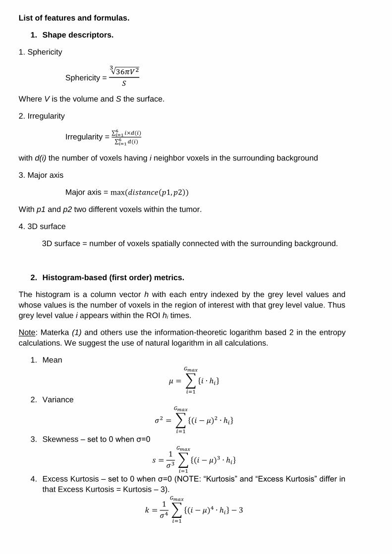
List of features and formulas.

1. Shape descriptors.

1. Sphericity

Sphericity = √36𝜋𝑉23

𝑆

Where V is the volume and S the surface.

2. Irregularity

Irregularity = ∑ 𝑖×𝑑(𝑖)6

𝑖=1

∑ 𝑑(𝑖)6𝑖=1

with d(i) the number of voxels having i neighbor voxels in the surrounding background

3. Major axis

Major axis = max(𝑑𝑖𝑠𝑡𝑎𝑛𝑐𝑒(𝑝1, 𝑝2))

With p1 and p2 two different voxels within the tumor.

4. 3D surface

3D surface = number of voxels spatially connected with the surrounding background.

2. Histogram-based (first order) metrics.

The histogram is a column vector h with each entry indexed by the grey level values and

whose values is the number of voxels in the region of interest with that grey level value. Thus

grey level value i appears within the ROI hi times.

Note: Materka (1) and others use the information-theoretic logarithm based 2 in the entropy

calculations. We suggest the use of natural logarithm in all calculations.

1. Mean

𝜇 = ∑ {𝑖 ∙ ℎ𝑖}

𝐺𝑚𝑎𝑥

𝑖=1

2. Variance

𝜎2 = ∑ {(𝑖 − 𝜇)2 ∙ ℎ𝑖}

𝐺𝑚𝑎𝑥

𝑖=1

3. Skewness – set to 0 when σ=0

𝑠 =1

𝜎3∑ {(𝑖 − 𝜇)3 ∙ ℎ𝑖}

𝐺𝑚𝑎𝑥

𝑖=1

4. Excess Kurtosis – set to 0 when σ=0 (NOTE: “Kurtosis” and “Excess Kurtosis” differ in

that Excess Kurtosis = Kurtosis – 3).

𝑘 =1

𝜎4∑ {(𝑖 − 𝜇)4 ∙ ℎ𝑖} − 3

𝐺𝑚𝑎𝑥

𝑖=1

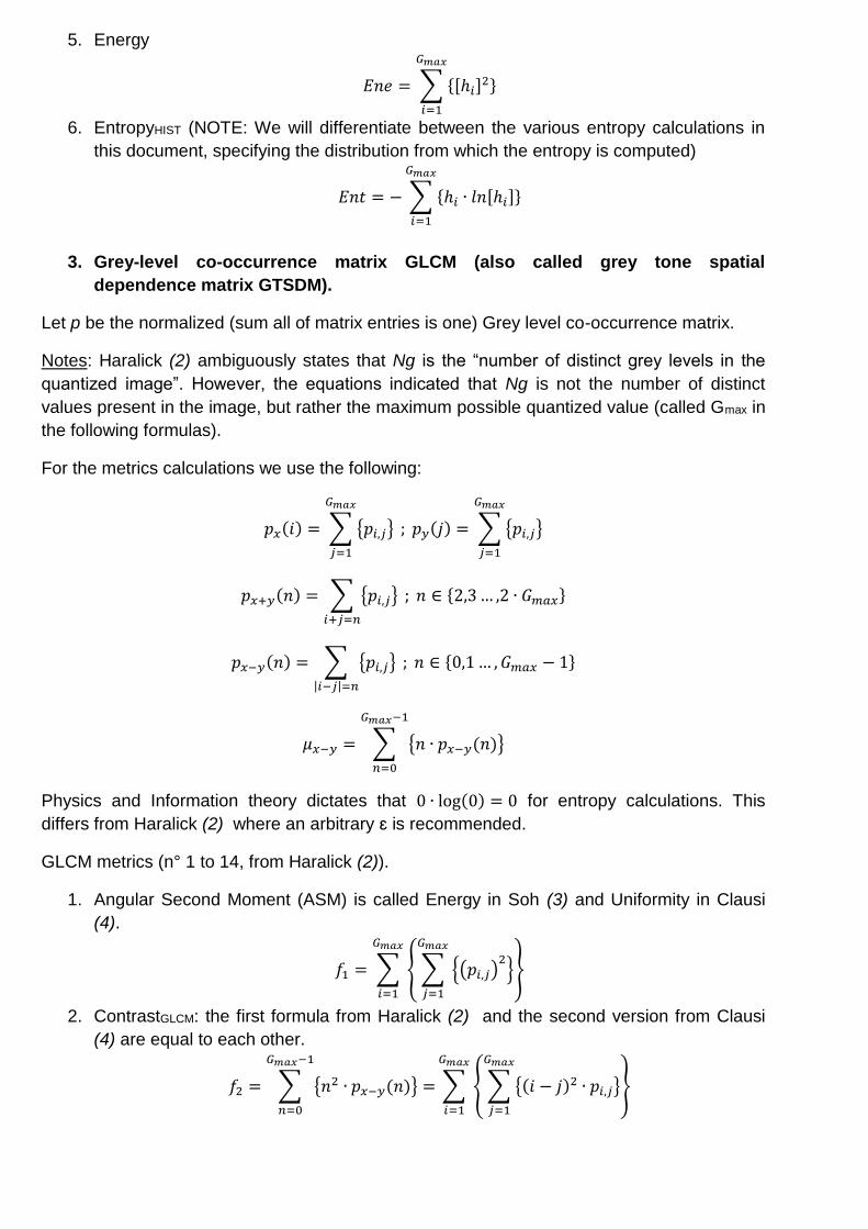
5. Energy

𝐸𝑛𝑒 = ∑ {[ℎ𝑖]2}

𝐺𝑚𝑎𝑥

𝑖=1

6. EntropyHIST (NOTE: We will differentiate between the various entropy calculations in

this document, specifying the distribution from which the entropy is computed)

𝐸𝑛𝑡 = − ∑ {ℎ𝑖 ∙ 𝑙𝑛[ℎ𝑖]}

𝐺𝑚𝑎𝑥

𝑖=1

3. Grey-level co-occurrence matrix GLCM (also called grey tone spatial

dependence matrix GTSDM).

Let p be the normalized (sum all of matrix entries is one) Grey level co-occurrence matrix.

Notes: Haralick (2) ambiguously states that Ng is the “number of distinct grey levels in the

quantized image”. However, the equations indicated that Ng is not the number of distinct

values present in the image, but rather the maximum possible quantized value (called Gmax in

the following formulas).

For the metrics calculations we use the following:

𝑝𝑥(𝑖) = ∑ {𝑝𝑖,𝑗}

𝐺𝑚𝑎𝑥

𝑗=1

; 𝑝𝑦(𝑗) = ∑ {𝑝𝑖,𝑗}

𝐺𝑚𝑎𝑥

𝑗=1

𝑝𝑥+𝑦(𝑛) = ∑ {𝑝𝑖,𝑗}

𝑖+𝑗=𝑛

; 𝑛 ∈ {2,3 … ,2 ∙ 𝐺𝑚𝑎𝑥}

𝑝𝑥−𝑦(𝑛) = ∑ {𝑝𝑖,𝑗}|𝑖−𝑗|=𝑛

; 𝑛 ∈ {0,1 … , 𝐺𝑚𝑎𝑥 − 1}

𝜇𝑥−𝑦 = ∑ {𝑛 ∙ 𝑝𝑥−𝑦(𝑛)}

𝐺𝑚𝑎𝑥−1

𝑛=0

Physics and Information theory dictates that 0 ∙ log(0) = 0 for entropy calculations. This

differs from Haralick (2) where an arbitrary ԑ is recommended.

GLCM metrics (n° 1 to 14, from Haralick (2)).

1. Angular Second Moment (ASM) is called Energy in Soh (3) and Uniformity in Clausi

(4).

𝑓1 = ∑ { ∑ {(𝑝𝑖,𝑗)2

}

𝐺𝑚𝑎𝑥

𝑗=1

}

𝐺𝑚𝑎𝑥

𝑖=1

2. ContrastGLCM: the first formula from Haralick (2) and the second version from Clausi

(4) are equal to each other.

𝑓2 = ∑ {𝑛2 ∙ 𝑝𝑥−𝑦(𝑛)} =

𝐺𝑚𝑎𝑥−1

𝑛=0

∑ { ∑ {(𝑖 − 𝑗)2 ∙ 𝑝𝑖,𝑗}

𝐺𝑚𝑎𝑥

𝑗=1

}

𝐺𝑚𝑎𝑥

𝑖=1

3. Correlation: the first version corresponds to equations from Haralick (2) and Soh (3)

which are equal to each other. The second one is from Clausi (4), the two are

equivalent.

𝑓3 =∑ {∑ {𝑖 ∙ 𝑗 ∙ 𝑝𝑖,𝑗}

𝐺𝑚𝑎𝑥𝑗=1 } − 𝜇𝑥 ∙ 𝜇𝑦

𝐺𝑚𝑎𝑥𝑖=1

𝜎𝑥 ∙ 𝜎𝑦=

∑ {∑ {(𝑖 − 𝜇𝑥) ∙ (𝑗 − 𝜇𝑦) ∙ 𝑝𝑖,𝑗}𝐺𝑚𝑎𝑥𝑗=1 }

𝐺𝑚𝑎𝑥𝑖=1

𝜎𝑥 ∙ 𝜎𝑦

μx, μy, σx, and σy are only loosely hinted at in Haralick (2). Taking the means and variances of

the px could be interpreted as taking the mean of the values of px as a set of numbers, rather

than the distribution mean. This would be an incorrect interpretation, and computing the

mean of the distribution is the correct interpretation. This is corroborated by Bharati (5). The

following definitions are taken from Bharati (5):

𝜇𝑥 = ∑ {𝑖 ∙ ∑ {𝑝𝑖,𝑗}

𝐺𝑚𝑎𝑥

𝑗=1

} ;

𝐺𝑚𝑎𝑥

𝑖=1

𝜇𝑦 = ∑ {𝑗 ∙ ∑ {𝑝𝑖,𝑗}

𝐺𝑚𝑎𝑥

𝑖=1

}

𝐺𝑚𝑎𝑥

𝑗=1

𝜎𝑥 = ( ∑ {(𝑖 − 𝜇𝑥)2 ∙ ∑ {𝑝𝑖,𝑗}

𝐺𝑚𝑎𝑥

𝑗=1

}

𝐺𝑚𝑎𝑥

𝑖=1

)

1/2

; 𝜎𝑦 = ( ∑ {(𝑗 − 𝜇𝑦)2 ∙ ∑ {𝑝𝑖,𝑗}

𝐺𝑚𝑎𝑥

𝑖=1

}

𝐺𝑚𝑎𝑥

𝑗=1

)

1/2

4. Sum of Squares Variance: ambiguous, as µ was not defined.

𝑓4 = ∑ { ∑ {(𝑖 − 𝜇)2 ∙ 𝑝𝑖,𝑗}

𝐺𝑚𝑎𝑥

𝑗=1

}

𝐺𝑚𝑎𝑥

𝑖=1

We use the following definition for µ:

𝜇 =∑ {∑ {𝑝𝑖,𝑗}

𝐺𝑚𝑎𝑥𝑗=1 }

𝐺𝑚𝑎𝑥𝑖=1

(𝐺𝑚𝑎𝑥)2

5. Inverse Different Moment (IDM) (is called Homogeneity in Soh (3)).

𝑓5 = ∑ { ∑ {1

1 + (𝑖 − 𝑗)2∙ 𝑝𝑖,𝑗}

𝐺𝑚𝑎𝑥

𝑗=1

}

𝐺𝑚𝑎𝑥

𝑖=1

6. Sum Average (SAVE).

𝑓6 = ∑ {𝑛 ∙ 𝑝𝑥+𝑦(𝑛)}

2∙𝐺𝑚𝑎𝑥

𝑛=2

7. Sum Variance (SVAR): the formula is Haralick (2) incorrectly uses f8, an error that has

propagated into many other papers and code implementations.

𝑓7 = ∑ {(𝑛 − 𝑓6)2 ∙ 𝑝𝑥+𝑦(𝑛)}

2∙𝐺𝑚𝑎𝑥

𝑛=2

8. GLCM Sum Entropy (SENT).

𝑓8 = − ∑ {𝑝𝑥+𝑦(𝑛) ∙ ln[𝑝𝑥+𝑦(𝑛)]}

2∙𝐺𝑚𝑎𝑥

𝑛=2

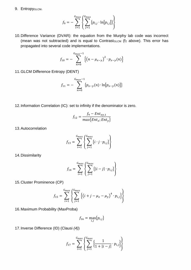
9. EntropyGLCM.

𝑓9 = − ∑ { ∑ {𝑝𝑖,𝑗 ∙ ln[𝑝𝑖,𝑗]}

𝐺𝑚𝑎𝑥

𝑗=1

}

𝐺𝑚𝑎𝑥

𝑖=1

10. Difference Variance (DVAR): the equation from the Murphy lab code was incorrect

(mean was not subtracted) and is equal to ContrastGLCM (f2 above). This error has

propagated into several code implementations.

𝑓10 = − ∑ {(𝑛 − 𝜇𝑥−𝑦)2

∙ 𝑝𝑥−𝑦(𝑛)}

𝐺𝑚𝑎𝑥−1

𝑛=0

11. GLCM Difference Entropy (DENT)

𝑓11 = − ∑ {𝑝𝑥−𝑦(𝑛) ∙ ln[𝑝𝑥−𝑦(𝑛)]}

𝐺𝑚𝑎𝑥−1

𝑛=0

12. Information Correlation (IC): set to infinity if the denominator is zero.

𝑓12 =𝑓9 − 𝐸𝑛𝑡𝑥𝑦,1

𝑚𝑎𝑥{𝐸𝑛𝑡𝑥; 𝐸𝑛𝑡𝑦}

13. Autocorrelation

𝑓13 = ∑ { ∑ {𝑖 ∙ 𝑗 ∙ 𝑝𝑖,𝑗}

𝐺𝑚𝑎𝑥

𝑗=1

}

𝐺𝑚𝑎𝑥

𝑖=1

14. Dissimilarity

𝑓14 = ∑ { ∑ {|𝑖 − 𝑗| ∙ 𝑝𝑖,𝑗}

𝐺𝑚𝑎𝑥

𝑗=1

}

𝐺𝑚𝑎𝑥

𝑖=1

15. Cluster Prominence (CP)

𝑓15 = ∑ { ∑ {(𝑖 + 𝑗 − 𝜇𝑥 − 𝜇𝑦)4

∙ 𝑝𝑖,𝑗}

𝐺𝑚𝑎𝑥

𝑗=1

}

𝐺𝑚𝑎𝑥

𝑖=1

16. Maximum Probability (MaxProba)

𝑓16 = max𝑖,𝑗

{𝑝𝑖,𝑗}

17. Inverse Difference (ID) (Clausi (4))

𝑓17 = ∑ { ∑ {1

1 + |𝑖 − 𝑗|∙ 𝑝𝑖,𝑗}

𝐺𝑚𝑎𝑥

𝑗=1

}

𝐺𝑚𝑎𝑥

𝑖=1

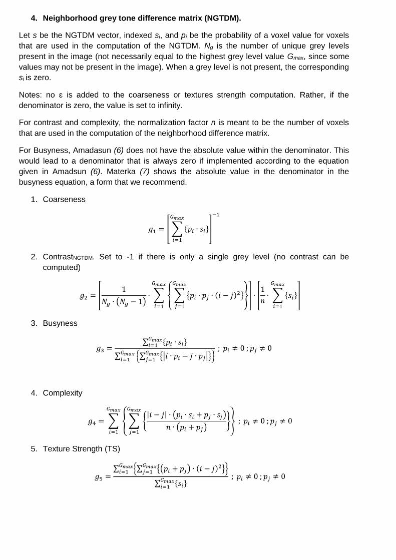
4. Neighborhood grey tone difference matrix (NGTDM).

Let s be the NGTDM vector, indexed si, and pi be the probability of a voxel value for voxels

that are used in the computation of the NGTDM. Ng is the number of unique grey levels

present in the image (not necessarily equal to the highest grey level value Gmax, since some

values may not be present in the image). When a grey level is not present, the corresponding

si is zero.

Notes: no ԑ is added to the coarseness or textures strength computation. Rather, if the

denominator is zero, the value is set to infinity.

For contrast and complexity, the normalization factor n is meant to be the number of voxels

that are used in the computation of the neighborhood difference matrix.

For Busyness, Amadasun (6) does not have the absolute value within the denominator. This

would lead to a denominator that is always zero if implemented according to the equation

given in Amadsun (6). Materka (7) shows the absolute value in the denominator in the

busyness equation, a form that we recommend.

1. Coarseness

𝑔1 = [ ∑ {𝑝𝑖 ∙ 𝑠𝑖}

𝐺𝑚𝑎𝑥

𝑖=1

]

−1

2. ContrastNGTDM. Set to -1 if there is only a single grey level (no contrast can be

computed)

𝑔2 = [1

𝑁𝑔 ∙ (𝑁𝑔 − 1)∙ ∑ { ∑ {𝑝𝑖 ∙ 𝑝𝑗 ∙ (𝑖 − 𝑗)2}

𝐺𝑚𝑎𝑥

𝑗=1

}

𝐺𝑚𝑎𝑥

𝑖=1

] ∙ [1

𝑛∙ ∑ {𝑠𝑖}

𝐺𝑚𝑎𝑥

𝑖=1

]

3. Busyness

𝑔3 =∑ {𝑝𝑖 ∙ 𝑠𝑖}𝐺𝑚𝑎𝑥

𝑖=1

∑ {∑ {|𝑖 ∙ 𝑝𝑖 − 𝑗 ∙ 𝑝𝑗|}𝐺𝑚𝑎𝑥

𝑗=1 }𝐺𝑚𝑎𝑥

𝑖=1

; 𝑝𝑖 ≠ 0 ; 𝑝𝑗 ≠ 0

4. Complexity

𝑔4 = ∑ { ∑ {|𝑖 − 𝑗| ∙ (𝑝𝑖 ∙ 𝑠𝑖 + 𝑝𝑗 ∙ 𝑠𝑗)

𝑛 ∙ (𝑝𝑖 + 𝑝𝑗)}

𝐺𝑚𝑎𝑥

𝑗=1

}

𝐺𝑚𝑎𝑥

𝑖=1

; 𝑝𝑖 ≠ 0 ; 𝑝𝑗 ≠ 0

5. Texture Strength (TS)

𝑔5 =∑ {∑ {(𝑝𝑖 + 𝑝𝑗) ∙ (𝑖 − 𝑗)2}

𝐺𝑚𝑎𝑥𝑗=1 }

𝐺𝑚𝑎𝑥𝑖=1

∑ {𝑠𝑖}𝐺𝑚𝑎𝑥

𝑖=1

; 𝑝𝑖 ≠ 0 ; 𝑝𝑗 ≠ 0

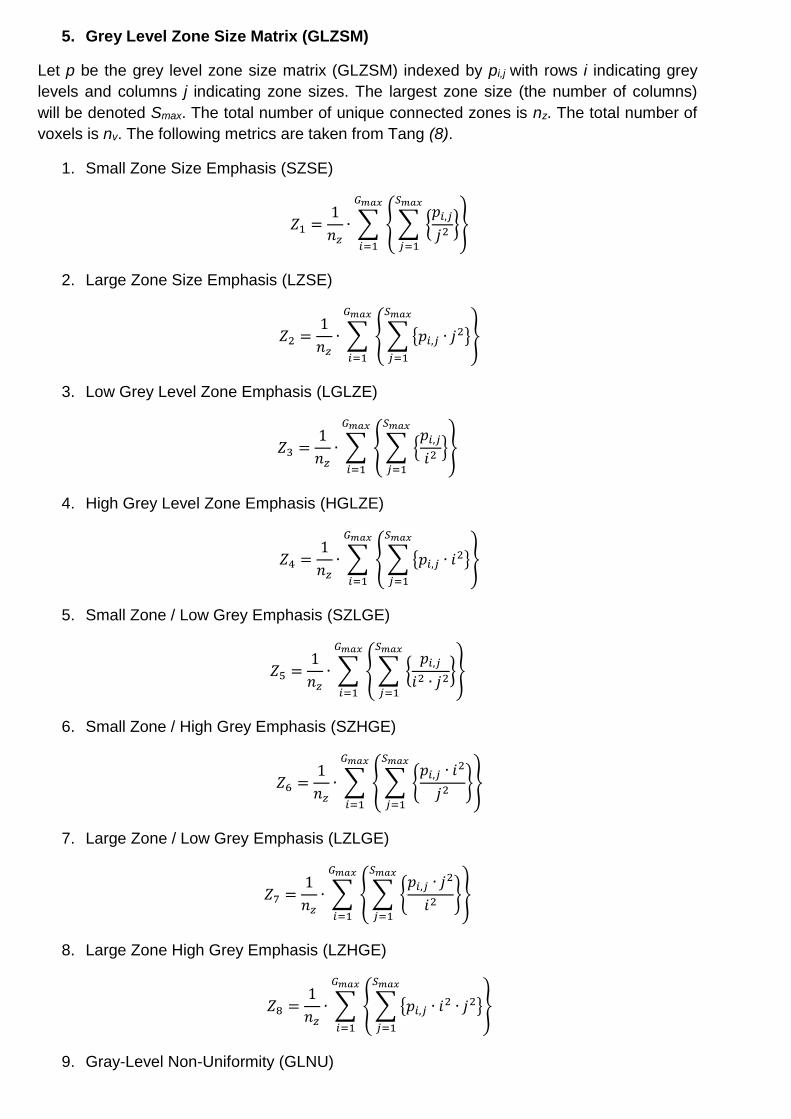
5. Grey Level Zone Size Matrix (GLZSM)

Let p be the grey level zone size matrix (GLZSM) indexed by pi,j with rows i indicating grey

levels and columns j indicating zone sizes. The largest zone size (the number of columns)

will be denoted Smax. The total number of unique connected zones is nz. The total number of

voxels is nv. The following metrics are taken from Tang (8).

1. Small Zone Size Emphasis (SZSE)

𝑍1 =1

𝑛𝑧∙ ∑ { ∑ {

𝑝𝑖,𝑗

𝑗2}

𝑆𝑚𝑎𝑥

𝑗=1

}

𝐺𝑚𝑎𝑥

𝑖=1

2. Large Zone Size Emphasis (LZSE)

𝑍2 =1

𝑛𝑧∙ ∑ { ∑ {𝑝𝑖,𝑗 ∙ 𝑗2}

𝑆𝑚𝑎𝑥

𝑗=1

}

𝐺𝑚𝑎𝑥

𝑖=1

3. Low Grey Level Zone Emphasis (LGLZE)

𝑍3 =1

𝑛𝑧∙ ∑ { ∑ {

𝑝𝑖,𝑗

𝑖2}

𝑆𝑚𝑎𝑥

𝑗=1

}

𝐺𝑚𝑎𝑥

𝑖=1

4. High Grey Level Zone Emphasis (HGLZE)

𝑍4 =1

𝑛𝑧∙ ∑ { ∑ {𝑝𝑖,𝑗 ∙ 𝑖2}

𝑆𝑚𝑎𝑥

𝑗=1

}

𝐺𝑚𝑎𝑥

𝑖=1

5. Small Zone / Low Grey Emphasis (SZLGE)

𝑍5 =1

𝑛𝑧∙ ∑ { ∑ {

𝑝𝑖,𝑗

𝑖2 ∙ 𝑗2}

𝑆𝑚𝑎𝑥

𝑗=1

}

𝐺𝑚𝑎𝑥

𝑖=1

6. Small Zone / High Grey Emphasis (SZHGE)

𝑍6 =1

𝑛𝑧∙ ∑ { ∑ {

𝑝𝑖,𝑗 ∙ 𝑖2

𝑗2}

𝑆𝑚𝑎𝑥

𝑗=1

}

𝐺𝑚𝑎𝑥

𝑖=1

7. Large Zone / Low Grey Emphasis (LZLGE)

𝑍7 =1

𝑛𝑧∙ ∑ { ∑ {

𝑝𝑖,𝑗 ∙ 𝑗2

𝑖2}

𝑆𝑚𝑎𝑥

𝑗=1

}

𝐺𝑚𝑎𝑥

𝑖=1

8. Large Zone High Grey Emphasis (LZHGE)

𝑍8 =1

𝑛𝑧∙ ∑ { ∑ {𝑝𝑖,𝑗 ∙ 𝑖2 ∙ 𝑗2}

𝑆𝑚𝑎𝑥

𝑗=1

}

𝐺𝑚𝑎𝑥

𝑖=1

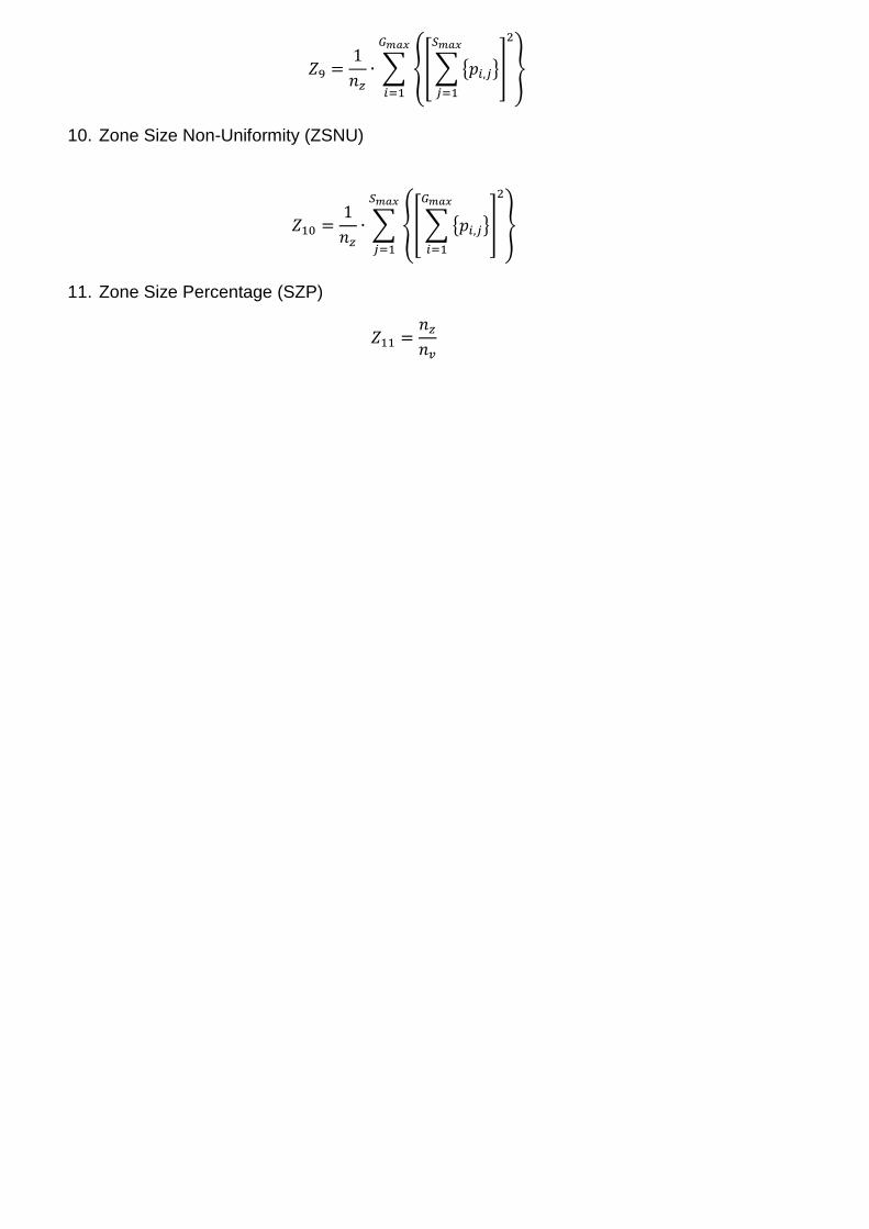
9. Gray-Level Non-Uniformity (GLNU)

𝑍9 =1

𝑛𝑧∙ ∑ {[ ∑ {𝑝𝑖,𝑗}

𝑆𝑚𝑎𝑥

𝑗=1

]

2

}

𝐺𝑚𝑎𝑥

𝑖=1

10. Zone Size Non-Uniformity (ZSNU)

𝑍10 =1

𝑛𝑧∙ ∑ {[ ∑ {𝑝𝑖,𝑗}

𝐺𝑚𝑎𝑥

𝑖=1

]

2

}

𝑆𝑚𝑎𝑥

𝑗=1

11. Zone Size Percentage (SZP)

𝑍11 =𝑛𝑧

𝑛𝑣

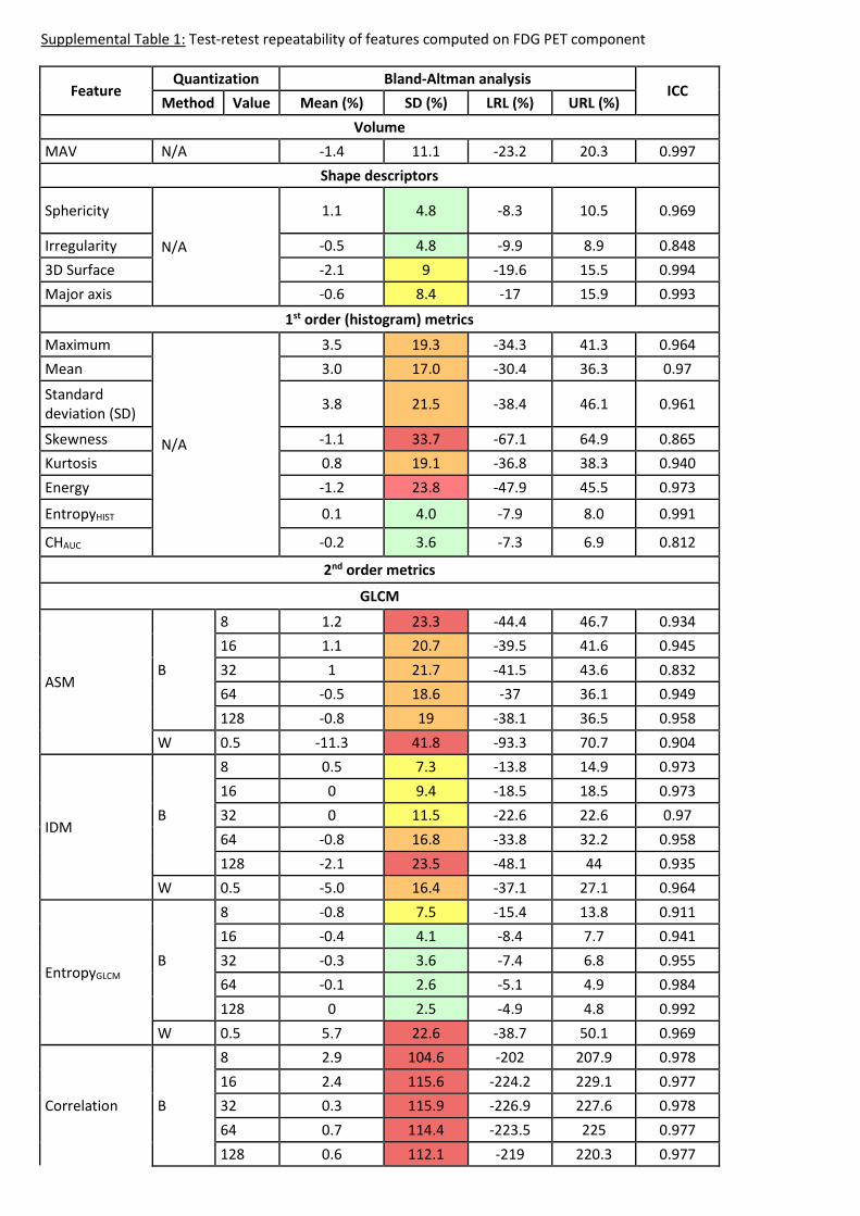
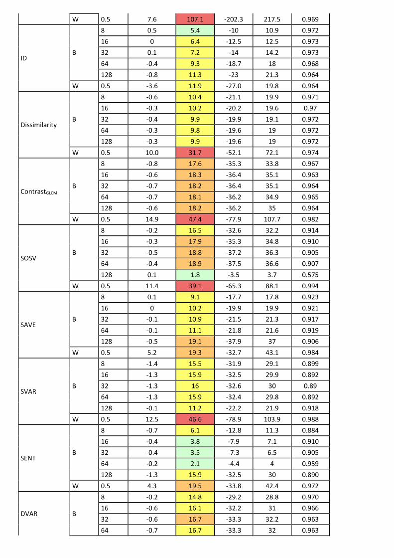
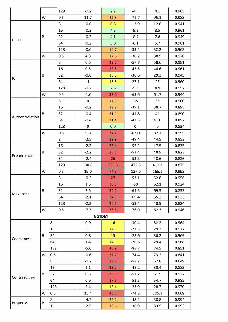
Supplemental Table 1: Test-retest repeatability of features computed on FDG PET component

Feature Quantization Bland-Altman analysis

ICC Method Value Mean (%) SD (%) LRL (%) URL (%)

Volume

MAV N/A -1.4 11.1 -23.2 20.3 0.997

Shape descriptors

Sphericity

N/A

1.1 4.8 -8.3 10.5 0.969

Irregularity -0.5 4.8 -9.9 8.9 0.848

3D Surface -2.1 9 -19.6 15.5 0.994

Major axis -0.6 8.4 -17 15.9 0.993

1st order (histogram) metrics

Maximum

N/A

3.5 19.3 -34.3 41.3 0.964

Mean 3.0 17.0 -30.4 36.3 0.97

Standard deviation (SD)

3.8 21.5 -38.4 46.1 0.961

Skewness -1.1 33.7 -67.1 64.9 0.865

Kurtosis 0.8 19.1 -36.8 38.3 0.940

Energy -1.2 23.8 -47.9 45.5 0.973

EntropyHIST 0.1 4.0 -7.9 8.0 0.991

CHAUC -0.2 3.6 -7.3 6.9 0.812

2nd order metrics

GLCM

ASM B

8 1.2 23.3 -44.4 46.7 0.934

16 1.1 20.7 -39.5 41.6 0.945

32 1 21.7 -41.5 43.6 0.832

64 -0.5 18.6 -37 36.1 0.949

128 -0.8 19 -38.1 36.5 0.958

W 0.5 -11.3 41.8 -93.3 70.7 0.904

IDM B

8 0.5 7.3 -13.8 14.9 0.973

16 0 9.4 -18.5 18.5 0.973

32 0 11.5 -22.6 22.6 0.97

64 -0.8 16.8 -33.8 32.2 0.958

128 -2.1 23.5 -48.1 44 0.935

W 0.5 -5.0 16.4 -37.1 27.1 0.964

EntropyGLCM B

8 -0.8 7.5 -15.4 13.8 0.911

16 -0.4 4.1 -8.4 7.7 0.941

32 -0.3 3.6 -7.4 6.8 0.955

64 -0.1 2.6 -5.1 4.9 0.984

128 0 2.5 -4.9 4.8 0.992

W 0.5 5.7 22.6 -38.7 50.1 0.969

Correlation B

8 2.9 104.6 -202 207.9 0.978

16 2.4 115.6 -224.2 229.1 0.977

32 0.3 115.9 -226.9 227.6 0.978

64 0.7 114.4 -223.5 225 0.977

128 0.6 112.1 -219 220.3 0.977

W 0.5 7.6 107.1 -202.3 217.5 0.969

ID B

8 0.5 5.4 -10 10.9 0.972

16 0 6.4 -12.5 12.5 0.973

32 0.1 7.2 -14 14.2 0.973

64 -0.4 9.3 -18.7 18 0.968

128 -0.8 11.3 -23 21.3 0.964

W 0.5 -3.6 11.9 -27.0 19.8 0.964

Dissimilarity B

8 -0.6 10.4 -21.1 19.9 0.971

16 -0.3 10.2 -20.2 19.6 0.97

32 -0.4 9.9 -19.9 19.1 0.972

64 -0.3 9.8 -19.6 19 0.972

128 -0.3 9.9 -19.6 19 0.972

W 0.5 10.0 31.7 -52.1 72.1 0.974

ContrastGLCM B

8 -0.8 17.6 -35.3 33.8 0.967

16 -0.6 18.3 -36.4 35.1 0.963

32 -0.7 18.2 -36.4 35.1 0.964

64 -0.7 18.1 -36.2 34.9 0.965

128 -0.6 18.2 -36.2 35 0.964

W 0.5 14.9 47.4 -77.9 107.7 0.982

SOSV B

8 -0.2 16.5 -32.6 32.2 0.914

16 -0.3 17.9 -35.3 34.8 0.910

32 -0.5 18.8 -37.2 36.3 0.905

64 -0.4 18.9 -37.5 36.6 0.907

128 0.1 1.8 -3.5 3.7 0.575

W 0.5 11.4 39.1 -65.3 88.1 0.994

SAVE B

8 0.1 9.1 -17.7 17.8 0.923

16 0 10.2 -19.9 19.9 0.921

32 -0.1 10.9 -21.5 21.3 0.917

64 -0.1 11.1 -21.8 21.6 0.919

128 -0.5 19.1 -37.9 37 0.906

W 0.5 5.2 19.3 -32.7 43.1 0.984

SVAR B

8 -1.4 15.5 -31.9 29.1 0.899

16 -1.3 15.9 -32.5 29.9 0.892

32 -1.3 16 -32.6 30 0.89

64 -1.3 15.9 -32.4 29.8 0.892

128 -0.1 11.2 -22.2 21.9 0.918

W 0.5 12.5 46.6 -78.9 103.9 0.988

SENT B

8 -0.7 6.1 -12.8 11.3 0.884

16 -0.4 3.8 -7.9 7.1 0.910

32 -0.4 3.5 -7.3 6.5 0.905

64 -0.2 2.1 -4.4 4 0.959

128 -1.3 15.9 -32.5 30 0.890

W 0.5 4.3 19.5 -33.8 42.4 0.972

DVAR B

8 -0.2 14.8 -29.2 28.8 0.970

16 -0.6 16.1 -32.2 31 0.966

32 -0.6 16.7 -33.3 32.2 0.963

64 -0.7 16.7 -33.3 32 0.963

128 -0.2 2.2 -4.5 4.1 0.965

W 0.5 11.7 42.5 -71.7 95.1 0.983

DENT B

8 -0.6 6.8 -13.9 12.8 0.941

16 -0.3 4.5 -9.2 8.5 0.961

32 -0.3 4.1 -8.4 7.8 0.949

64 -0.2 3.0 -6.1 5.7 0.961

128 -0.6 16.7 -33.4 32.2 0.963

W 0.5 4.3 17.6 -30.2 38.9 0.970

IC B

8 0.5 29.7 -57.7 58.6 0.981

16 0.5 22.5 -43.5 44.6 0.961

32 -0.6 15.3 -30.6 29.3 0.945

64 -1 13.3 -27.1 25 0.960

128 -0.2 2.6 -5.3 4.9 0.957

W 0.5 -1.0 32.0 -63.6 61.7 0.944

Autocorrelation B

8 0 17.9 -35 35 0.900

16 -0.2 19.8 -39.1 38.7 0.895

32 -0.4 21.1 -41.8 41 0.890

64 -0.4 21.4 -42.3 41.6 0.892

128 0 0.0 0 0 0.834

W 0.5 9.8 37.2 -63.0 82.7 0.995

Prominence B

8 -2.5 23.9 -49.4 44.5 0.853

16 -2.3 25.4 -52.2 47.5 0.835

32 -2.2 26.1 -53.4 48.9 0.823

64 -2.4 26 -53.3 48.6 0.826

128 -30.8 225.5 -472.8 411.1 0.875

W 0.5 19.0 74.5 -127.0 165.1 0.993

MaxProba B

8 -0.2 27 -53.1 52.8 0.956

16 1.5 30.9 -59 62.1 0.924

32 2.5 34.2 -64.5 69.5 0.833

64 -2.1 34.3 -69.4 65.2 0.933

128 -2.2 26.1 -53.4 48.9 0.824

W 0.5 -7.3 35.5 -76.9 62.3 0.946

NGTDM

Coarseness B

8 0.9 16 -30.4 32.2 0.964

16 1 14.5 -27.3 29.3 0.977

32 0.8 15 -28.6 30.2 0.969

64 1.4 14.3 -26.6 29.4 0.968

128 -5.6 40.9 -85.7 74.5 0.851

W 0.5 -0.6 37.7 -74.4 73.2 0.841

ContrastNGTDM B

8 -0.2 29.6 -58.2 57.8 0.649

16 1.1 25.2 -48.2 50.4 0.883

32 0.3 26.3 -51.2 51.9 0.927

64 0.6 27.6 -53.5 54.7 0.985

128 2.4 13.4 -23.9 28.7 0.970

W 0.5 15.4 45.7 -74.2 105.1 0.669

Busyness B 8 -4.7 22.2 -48.2 38.8 0.994

16 -2.5 18.6 -38.9 33.9 0.993

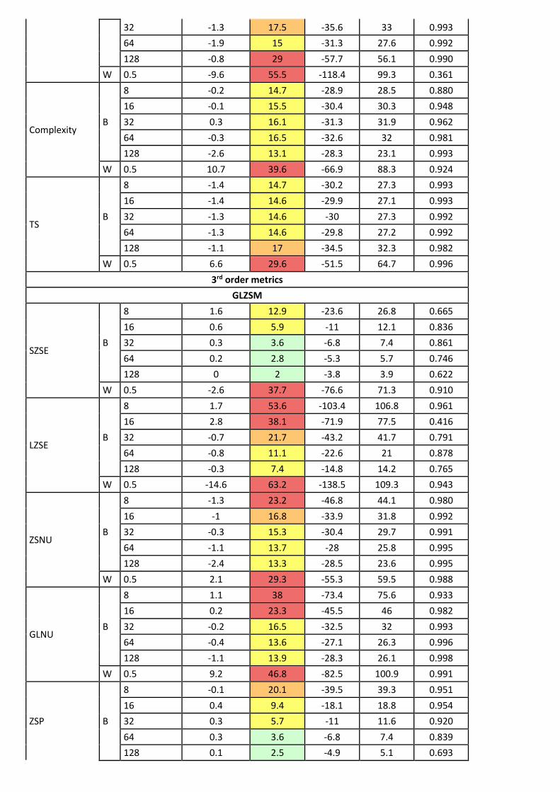
32 -1.3 17.5 -35.6 33 0.993

64 -1.9 15 -31.3 27.6 0.992

128 -0.8 29 -57.7 56.1 0.990

W 0.5 -9.6 55.5 -118.4 99.3 0.361

Complexity B

8 -0.2 14.7 -28.9 28.5 0.880

16 -0.1 15.5 -30.4 30.3 0.948

32 0.3 16.1 -31.3 31.9 0.962

64 -0.3 16.5 -32.6 32 0.981

128 -2.6 13.1 -28.3 23.1 0.993

W 0.5 10.7 39.6 -66.9 88.3 0.924

TS B

8 -1.4 14.7 -30.2 27.3 0.993

16 -1.4 14.6 -29.9 27.1 0.993

32 -1.3 14.6 -30 27.3 0.992

64 -1.3 14.6 -29.8 27.2 0.992

128 -1.1 17 -34.5 32.3 0.982

W 0.5 6.6 29.6 -51.5 64.7 0.996

3rd order metrics

GLZSM

SZSE B

8 1.6 12.9 -23.6 26.8 0.665

16 0.6 5.9 -11 12.1 0.836

32 0.3 3.6 -6.8 7.4 0.861

64 0.2 2.8 -5.3 5.7 0.746

128 0 2 -3.8 3.9 0.622

W 0.5 -2.6 37.7 -76.6 71.3 0.910

LZSE B

8 1.7 53.6 -103.4 106.8 0.961

16 2.8 38.1 -71.9 77.5 0.416

32 -0.7 21.7 -43.2 41.7 0.791

64 -0.8 11.1 -22.6 21 0.878

128 -0.3 7.4 -14.8 14.2 0.765

W 0.5 -14.6 63.2 -138.5 109.3 0.943

ZSNU B

8 -1.3 23.2 -46.8 44.1 0.980

16 -1 16.8 -33.9 31.8 0.992

32 -0.3 15.3 -30.4 29.7 0.991

64 -1.1 13.7 -28 25.8 0.995

128 -2.4 13.3 -28.5 23.6 0.995

W 0.5 2.1 29.3 -55.3 59.5 0.988

GLNU B

8 1.1 38 -73.4 75.6 0.933

16 0.2 23.3 -45.5 46 0.982

32 -0.2 16.5 -32.5 32 0.993

64 -0.4 13.6 -27.1 26.3 0.996

128 -1.1 13.9 -28.3 26.1 0.998

W 0.5 9.2 46.8 -82.5 100.9 0.991

ZSP B

8 -0.1 20.1 -39.5 39.3 0.951

16 0.4 9.4 -18.1 18.8 0.954

32 0.3 5.7 -11 11.6 0.920

64 0.3 3.6 -6.8 7.4 0.839

128 0.1 2.5 -4.9 5.1 0.693

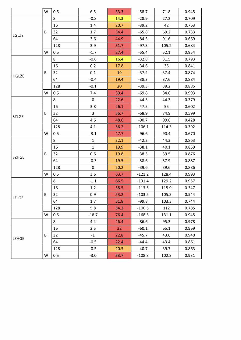
W 0.5 6.5 33.3 -58.7 71.8 0.945

LGLZE B

8 -0.8 14.3 -28.9 27.2 0.709

16 1.4 20.7 -39.2 42 0.763

32 1.7 34.4 -65.8 69.2 0.733

64 3.6 44.9 -84.5 91.6 0.669

128 3.9 51.7 -97.3 105.2 0.684

W 0.5 -1.7 27.4 -55.4 52.1 0.954

HGLZE B

8 -0.6 16.4 -32.8 31.5 0.793

16 0.2 17.8 -34.6 35 0.841

32 0.1 19 -37.2 37.4 0.874

64 -0.4 19.4 -38.3 37.6 0.884

128 -0.1 20 -39.3 39.2 0.885

W 0.5 7.4 39.4 -69.8 84.6 0.993

SZLGE B

8 0 22.6 -44.3 44.3 0.379

16 3.8 26.1 -47.5 55 0.602

32 3 36.7 -68.9 74.9 0.599

64 4.6 48.6 -90.7 99.8 0.428

128 4.1 56.2 -106.1 114.3 0.392

W 0.5 -3.1 47.7 -96.6 90.4 0.670

SZHGE B

8 1 22.1 -42.2 44.3 0.863

16 1 19.9 -38.1 40.1 0.859

32 0.6 19.8 -38.3 39.5 0.876

64 -0.3 19.5 -38.6 37.9 0.887

128 0 20.2 -39.6 39.6 0.886

W 0.5 3.6 63.7 -121.2 128.4 0.993

LZLGE B

8 -1.1 66.5 -131.4 129.2 0.957

16 1.2 58.5 -113.5 115.9 0.347

32 0.9 53.2 -103.5 105.3 0.544

64 1.7 51.8 -99.8 103.3 0.744

128 5.8 54.2 -100.5 112 0.785

W 0.5 -18.7 76.4 -168.5 131.1 0.945

LZHGE B

8 4.4 46.4 -86.6 95.3 0.978

16 2.5 32 -60.1 65.1 0.969

32 -1 22.8 -45.7 43.6 0.940

64 -0.5 22.4 -44.4 43.4 0.861

128 -0.5 20.5 -40.7 39.7 0.863

W 0.5 -3.0 53.7 -108.3 102.3 0.931

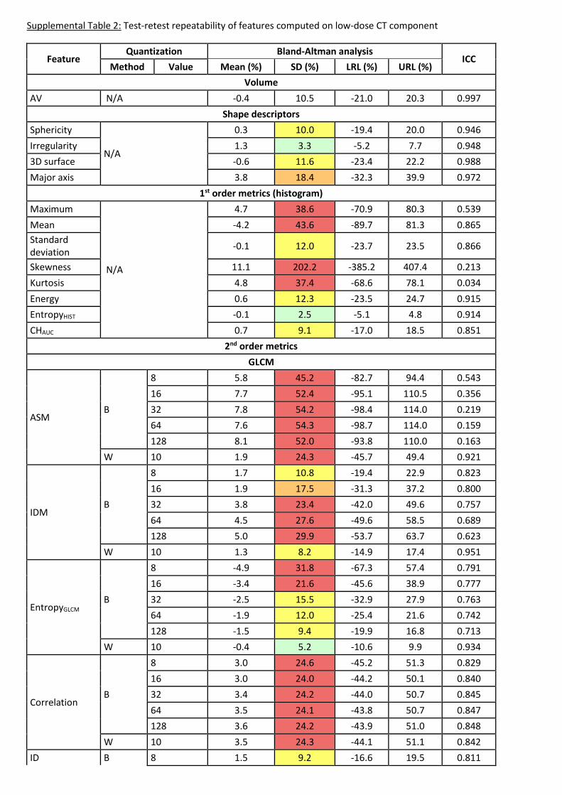
Supplemental Table 2: Test-retest repeatability of features computed on low-dose CT component

Feature Quantization Bland-Altman analysis

ICC Method Value Mean (%) SD (%) LRL (%) URL (%)

Volume

AV N/A -0.4 10.5 -21.0 20.3 0.997

Shape descriptors

Sphericity

N/A

0.3 10.0 -19.4 20.0 0.946

Irregularity 1.3 3.3 -5.2 7.7 0.948

3D surface -0.6 11.6 -23.4 22.2 0.988

Major axis 3.8 18.4 -32.3 39.9 0.972

1st order metrics (histogram)

Maximum

N/A

4.7 38.6 -70.9 80.3 0.539

Mean -4.2 43.6 -89.7 81.3 0.865

Standard deviation

-0.1 12.0 -23.7 23.5 0.866

Skewness 11.1 202.2 -385.2 407.4 0.213

Kurtosis 4.8 37.4 -68.6 78.1 0.034

Energy 0.6 12.3 -23.5 24.7 0.915

EntropyHIST -0.1 2.5 -5.1 4.8 0.914

CHAUC 0.7 9.1 -17.0 18.5 0.851

2nd order metrics

GLCM

ASM B

8 5.8 45.2 -82.7 94.4 0.543

16 7.7 52.4 -95.1 110.5 0.356

32 7.8 54.2 -98.4 114.0 0.219

64 7.6 54.3 -98.7 114.0 0.159

128 8.1 52.0 -93.8 110.0 0.163

W 10 1.9 24.3 -45.7 49.4 0.921

IDM B

8 1.7 10.8 -19.4 22.9 0.823

16 1.9 17.5 -31.3 37.2 0.800

32 3.8 23.4 -42.0 49.6 0.757

64 4.5 27.6 -49.6 58.5 0.689

128 5.0 29.9 -53.7 63.7 0.623

W 10 1.3 8.2 -14.9 17.4 0.951

EntropyGLCM B

8 -4.9 31.8 -67.3 57.4 0.791

16 -3.4 21.6 -45.6 38.9 0.777

32 -2.5 15.5 -32.9 27.9 0.763

64 -1.9 12.0 -25.4 21.6 0.742

128 -1.5 9.4 -19.9 16.8 0.713

W 10 -0.4 5.2 -10.6 9.9 0.934

Correlation B

8 3.0 24.6 -45.2 51.3 0.829

16 3.0 24.0 -44.2 50.1 0.840

32 3.4 24.2 -44.0 50.7 0.845

64 3.5 24.1 -43.8 50.7 0.847

128 3.6 24.2 -43.9 51.0 0.848

W 10 3.5 24.3 -44.1 51.1 0.842

ID B 8 1.5 9.2 -16.6 19.5 0.811

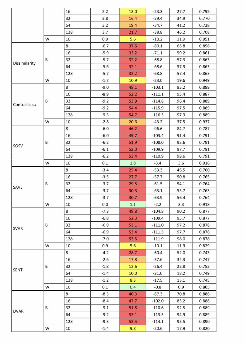
16 2.2 13.0 -23.3 27.7 0.795

32 2.8 16.4 -29.4 34.9 0.770

64 3.2 19.4 -34.7 41.2 0.738

128 3.7 21.7 -38.8 46.2 0.708

W 10 0.9 5.6 -10.2 11.9 0.951

Dissimilarity B

8 -6.7 37.5 -80.1 66.8 0.856

16 -5.9 33.2 -71.1 59.2 0.861

32 -5.7 32.2 -68.8 57.3 0.863

64 -5.6 32.1 -68.6 57.3 0.863

128 -5.7 32.2 -68.8 57.4 0.863

W 10 -1.7 10.9 -23.0 19.6 0.949

ContrastGLCM

B

8 -9.0 48.1 -103.1 85.2 0.889

16 -8.9 52.2 -111.1 93.4 0.887

32 -9.2 53.9 -114.8 96.4 0.889

64 -9.2 54.4 -115.9 97.5 0.889

128 -9.3 54.7 -116.5 97.9 0.889

W 10 -2.8 20.6 -43.2 37.5 0.937

SOSV B

8 -6.0 46.2 -96.6 84.7 0.787

16 -6.0 49.7 -103.4 91.4 0.791

32 -6.2 51.9 -108.0 95.6 0.791

64 -6.1 53.0 -109.9 97.7 0.791

128 -6.2 53.4 -110.9 98.6 0.791

W 10 0.1 1.8 -3.4 3.6 0.916

SAVE B

8 -3.4 25.4 -53.3 46.5 0.760

16 -3.5 27.7 -57.7 50.8 0.765

32 -3.7 29.5 -61.5 54.1 0.764

64 -3.7 30.3 -63.1 55.7 0.763

128 -3.7 30.7 -63.9 56.4 0.764

W 10 0.0 1.1 -2.2 2.3 0.918

SVAR B

8 -7.3 49.8 -104.8 90.2 0.877

16 -6.8 52.3 -109.4 95.7 0.877

32 -6.9 53.1 -111.0 97.2 0.878

64 -6.9 53.4 -111.5 97.7 0.878

128 -7.0 53.5 -111.9 98.0 0.878

W 10 0.9 5.6 -10.1 11.9 0.829

SENT B

8 -4.2 28.7 -60.4 52.0 0.743

16 -2.6 17.8 -37.6 32.3 0.747

32 -1.8 12.6 -26.4 22.8 0.752

64 -1.4 10.0 -21.0 18.2 0.749

128 -1.2 8.3 -17.5 15.1 0.745

W 10 0.1 0.4 -0.8 0.9 0.865

DVAR B

8 -8.3 40.3 -87.3 70.8 0.886

16 -8.4 47.7 -102.0 85.2 0.888

32 -9.1 51.8 -110.6 92.5 0.889

64 -9.2 53.1 -113.3 94.9 0.889

128 -9.3 53.5 -114.1 95.5 0.890

W 10 -1.4 9.8 -20.6 17.9 0.820

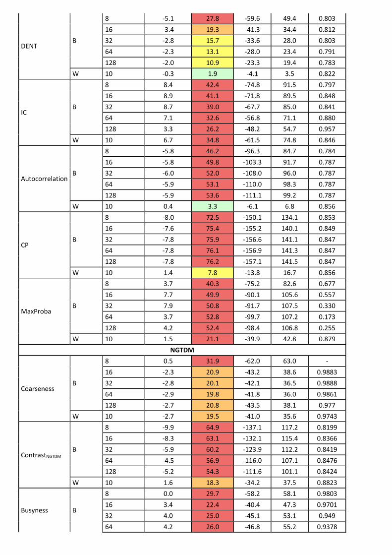
DENT B

8 -5.1 27.8 -59.6 49.4 0.803

16 -3.4 19.3 -41.3 34.4 0.812

32 -2.8 15.7 -33.6 28.0 0.803

64 -2.3 13.1 -28.0 23.4 0.791

128 -2.0 10.9 -23.3 19.4 0.783

W 10 -0.3 1.9 -4.1 3.5 0.822

IC B

8 8.4 42.4 -74.8 91.5 0.797

16 8.9 41.1 -71.8 89.5 0.848

32 8.7 39.0 -67.7 85.0 0.841

64 7.1 32.6 -56.8 71.1 0.880

128 3.3 26.2 -48.2 54.7 0.957

W 10 6.7 34.8 -61.5 74.8 0.846

Autocorrelation B

8 -5.8 46.2 -96.3 84.7 0.784

16 -5.8 49.8 -103.3 91.7 0.787

32 -6.0 52.0 -108.0 96.0 0.787

64 -5.9 53.1 -110.0 98.3 0.787

128 -5.9 53.6 -111.1 99.2 0.787

W 10 0.4 3.3 -6.1 6.8 0.856

CP B

8 -8.0 72.5 -150.1 134.1 0.853

16 -7.6 75.4 -155.2 140.1 0.849

32 -7.8 75.9 -156.6 141.1 0.847

64 -7.8 76.1 -156.9 141.3 0.847

128 -7.8 76.2 -157.1 141.5 0.847

W 10 1.4 7.8 -13.8 16.7 0.856

MaxProba B

8 3.7 40.3 -75.2 82.6 0.677

16 7.7 49.9 -90.1 105.6 0.557

32 7.9 50.8 -91.7 107.5 0.330

64 3.7 52.8 -99.7 107.2 0.173

128 4.2 52.4 -98.4 106.8 0.255

W 10 1.5 21.1 -39.9 42.8 0.879

NGTDM

Coarseness B

8 0.5 31.9 -62.0 63.0 -

16 -2.3 20.9 -43.2 38.6 0.9883

32 -2.8 20.1 -42.1 36.5 0.9888

64 -2.9 19.8 -41.8 36.0 0.9861

128 -2.7 20.8 -43.5 38.1 0.977

W 10 -2.7 19.5 -41.0 35.6 0.9743

ContrastNGTDM

B

8 -9.9 64.9 -137.1 117.2 0.8199

16 -8.3 63.1 -132.1 115.4 0.8366

32 -5.9 60.2 -123.9 112.2 0.8419

64 -4.5 56.9 -116.0 107.1 0.8476

128 -5.2 54.3 -111.6 101.1 0.8424

W 10 1.6 18.3 -34.2 37.5 0.8823

Busyness B

8 0.0 29.7 -58.2 58.1 0.9803

16 3.4 22.4 -40.4 47.3 0.9701

32 4.0 25.0 -45.1 53.1 0.949

64 4.2 26.0 -46.8 55.2 0.9378

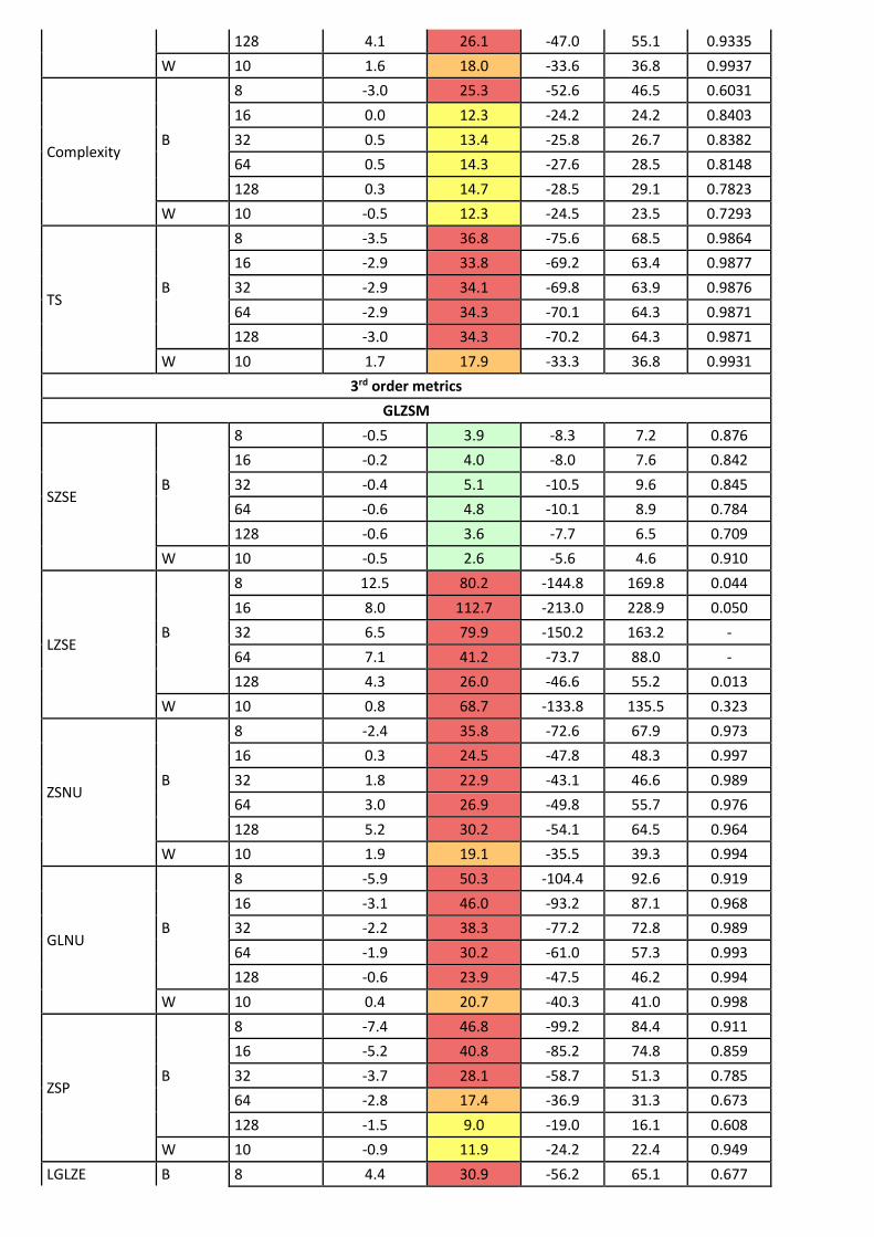
128 4.1 26.1 -47.0 55.1 0.9335

W 10 1.6 18.0 -33.6 36.8 0.9937

Complexity B

8 -3.0 25.3 -52.6 46.5 0.6031

16 0.0 12.3 -24.2 24.2 0.8403

32 0.5 13.4 -25.8 26.7 0.8382

64 0.5 14.3 -27.6 28.5 0.8148

128 0.3 14.7 -28.5 29.1 0.7823

W 10 -0.5 12.3 -24.5 23.5 0.7293

TS B

8 -3.5 36.8 -75.6 68.5 0.9864

16 -2.9 33.8 -69.2 63.4 0.9877

32 -2.9 34.1 -69.8 63.9 0.9876

64 -2.9 34.3 -70.1 64.3 0.9871

128 -3.0 34.3 -70.2 64.3 0.9871

W 10 1.7 17.9 -33.3 36.8 0.9931

3rd order metrics

GLZSM

SZSE B

8 -0.5 3.9 -8.3 7.2 0.876

16 -0.2 4.0 -8.0 7.6 0.842

32 -0.4 5.1 -10.5 9.6 0.845

64 -0.6 4.8 -10.1 8.9 0.784

128 -0.6 3.6 -7.7 6.5 0.709

W 10 -0.5 2.6 -5.6 4.6 0.910

LZSE B

8 12.5 80.2 -144.8 169.8 0.044

16 8.0 112.7 -213.0 228.9 0.050

32 6.5 79.9 -150.2 163.2 -

64 7.1 41.2 -73.7 88.0 -

128 4.3 26.0 -46.6 55.2 0.013

W 10 0.8 68.7 -133.8 135.5 0.323

ZSNU B

8 -2.4 35.8 -72.6 67.9 0.973

16 0.3 24.5 -47.8 48.3 0.997

32 1.8 22.9 -43.1 46.6 0.989

64 3.0 26.9 -49.8 55.7 0.976

128 5.2 30.2 -54.1 64.5 0.964

W 10 1.9 19.1 -35.5 39.3 0.994

GLNU B

8 -5.9 50.3 -104.4 92.6 0.919

16 -3.1 46.0 -93.2 87.1 0.968

32 -2.2 38.3 -77.2 72.8 0.989

64 -1.9 30.2 -61.0 57.3 0.993

128 -0.6 23.9 -47.5 46.2 0.994

W 10 0.4 20.7 -40.3 41.0 0.998

ZSP B

8 -7.4 46.8 -99.2 84.4 0.911

16 -5.2 40.8 -85.2 74.8 0.859

32 -3.7 28.1 -58.7 51.3 0.785

64 -2.8 17.4 -36.9 31.3 0.673

128 -1.5 9.0 -19.0 16.1 0.608

W 10 -0.9 11.9 -24.2 22.4 0.949

LGLZE B 8 4.4 30.9 -56.2 65.1 0.677

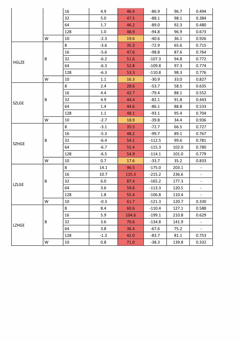
16 4.9 46.9 -86.9 96.7 0.494

32 5.0 47.5 -88.1 98.1 0.384

64 1.7 46.2 -89.0 92.3 0.480

128 1.0 48.9 -94.8 96.9 0.673

W 10 -2.3 19.6 -40.6 36.1 0.926

HGLZE B

8 -3.6 35.3 -72.9 65.6 0.715

16 -5.6 47.6 -98.8 87.6 0.764

32 -6.2 51.6 -107.3 94.8 0.772

64 -6.3 52.8 -109.8 97.3 0.774

128 -6.3 53.3 -110.8 98.3 0.776

W 10 1.1 16.3 -30.9 33.0 0.827

SZLGE B

8 2.4 28.6 -53.7 58.5 0.635

16 4.4 42.7 -79.4 88.1 0.552

32 4.9 44.4 -82.1 91.8 0.443

64 1.4 44.6 -86.1 88.8 0.533

128 1.1 48.1 -93.1 95.4 0.704

W 10 -2.7 18.9 -39.8 34.4 0.936

SZHGE B

8 -3.1 35.5 -72.7 66.5 0.727

16 -5.3 48.2 -99.7 89.1 0.767

32 -6.4 54.1 -112.5 99.6 0.781

64 -6.7 55.4 -115.3 102.0 0.780

128 -6.5 54.9 -114.1 101.0 0.779

W 10 0.7 17.6 -33.7 35.2 0.833

LZLGE B

8 14.1 96.5 -175.0 203.1 -

16 10.7 115.3 -215.2 236.6 -

32 6.0 87.4 -165.2 177.3 -

64 3.6 59.6 -113.3 120.5 -

128 1.8 55.4 -106.8 110.4 -

W 10 -0.3 61.7 -121.3 120.7 0.330

LZHGE B

8 8.4 60.6 -110.4 127.1 0.588

16 5.9 104.6 -199.1 210.8 0.629

32 3.6 70.6 -134.8 141.9 -

64 3.8 36.4 -67.6 75.2 -

128 -1.3 42.0 -83.7 81.1 0.753

W 10 0.8 71.0 -38.3 139.8 0.332

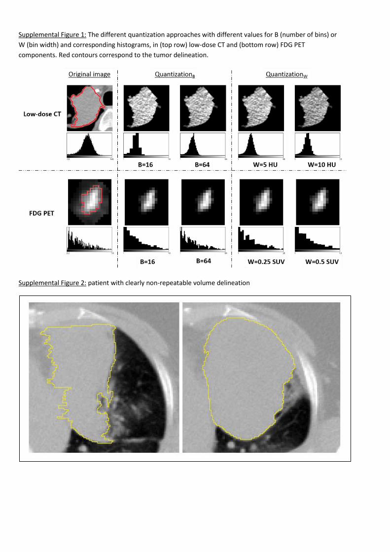
Supplemental Figure 1: The different quantization approaches with different values for B (number of bins) or

W (bin width) and corresponding histograms, in (top row) low-dose CT and (bottom row) FDG PET

components. Red contours correspond to the tumor delineation.

Supplemental Figure 2: patient with clearly non-repeatable volume delineation

REFERENCES

1. Materka A, Strzelecki M. Texture analysis methods – a review. INSTITUTE OF ELECTRONICS, TECHNICAL UNIVERSITY OF LODZ; 1998.

2. Haralick RM, Shanmugam K, Dinstein I. Textural Features for Image Classification. IEEE Trans Syst Man Cybern. 1973;SMC-3:610–621.

3. Soh L-K, Tsatsoulis C. Texture analysis of SAR sea ice imagery using gray level co-occurrence matrices. IEEE Trans Geosci Remote Sens. 1999;37(2):780–795.

4. Clausi DA. An analysis of co-occurrence texture statistics as a function of grey level quantization. Can J Remote Sens. 2002;28:45–62.

5. Bharati MH, Liu JJ, MacGregor JF. Image texture analysis: methods and comparisons. Chemom Intell Lab Syst. 2004;72:57–71.

6. Amadasun M, King R. Textural features corresponding to textural properties. IEEE Trans Syst Man Cybern. 1989;19:1264–1274.

7. Materka A, Strzelecki M, others. Texture analysis methods–a review. Tech Univ Lodz Inst Electron COST B11 Rep Bruss. 1998:9–11.

8. Tang X. Texture information in run-length matrices. IEEE Trans Image Process. 1998;7:1602–1609.