liquid nitrogen propulsion systems for automotive applications
TRANSCRIPT

LIQUID NITROGEN PROPULSION SYSTEMS FOR AUTOMOTIVE APPLICATIONS:
CALCULATION OF THE MECHANICAL EFFICIENCY OF A DUAL,
DOUBLE-ACTING PISTON PROPULSION SYSTEM
Thomas B. North, B.B.A., M.B.A.
Thesis Prepared for the Degree of
MASTER OF SCIENCE
UNIVERSITY OF NORTH TEXAS
May 2008
APPROVED: Mitty C. Plummer, Major Professor Philip Foster, Committee Member Seifollah Nazrazadani, Committee Member Nourredine Boubekri, Chair of the Department of
Engineering Technology Oscar García, Dean of the College of Engineering Sandra L. Terrell, Dean of the Robert B. Toulouse
School of Graduate Studies

North, Thomas B., Liquid Nitrogen Propulsion Systems for Automotive Applications:
Calculation of the Mechanical Efficiency of a Dual, Double-Acting Piston Propulsion System.
Master of Science (Engineering Technology), May 2008, 39 pp., 4 tables, 15 illustrations,
references, 19 titles.
A dual, double-acting propulsion system is analyzed to determine how efficiently it can
convert the potential energy available from liquid nitrogen into useful work. The two double-
acting pistons (high- and low-pressure) were analyzed by using a Matlab-Simulink computer
simulation to determine their respective mechanical efficiencies. The flow circuit for the entire
system was analyzed by using flow circuit analysis software to determine pressure losses
throughout the system at the required mass flow rates. The results of the piston simulation
indicate that the two pistons analyzed are very efficient at transferring energy into useful work.
The flow circuit analysis shows that the system can adequately maintain the mass flow rate
requirements of the pistons but also identifies components that have a significant impact on the
performance of the system. The results of the analysis indicate that the nitrogen propulsion
system meets the intended goals of its designers.

Copyright 2008
by
Thomas B. North
ii

ACKNOWLEDGEMENTS
First and foremost, I would like to thank my major professor, Dr. Mitty C. Plummer, for
his patience, guidance, wisdom, and wealth of knowledge, which have contributed immensely
toward my research work. My sincere gratitude goes to Dr. Philip Foster and Dr. Seifollah
Nazrazadani for being my thesis committee members and for giving their valuable time to guide
me and to review my thesis.
I would also like to thank Dr. Igor N. Kudryavtsev for his assistance with the MATLAB-
Simulink computer simulation and Mr. Jerry Davis for his assistance with the flow circuit
analysis software.
I am also indebted to my parents, family, and friends for their constant encouragement,
patience, and moral support throughout my educational endeavors.
iii

TABLE OF CONTENTS
Page ACKNOWLEDGEMENTS ........................................................................................................... iii LIST OF TABLES ......................................................................................................................... vi LIST OF FIGURES ...................................................................................................................... vii Chapters
1. INTRODUCTION ...................................................................................................1
Background of the Problem and Statement of Need ....................................1
Purpose of the Study ....................................................................................2
Statement of the Problem .............................................................................2
Scope of the Study .......................................................................................2
Significance of the Study .............................................................................4
Research Questions ......................................................................................4
Methodology ................................................................................................5
Limitations ...................................................................................................8
Assumptions .................................................................................................9 2. REVIEW OF THE LITERATURE .......................................................................10
Cryogenic Heat Engines ............................................................................12
Double-Acting Piston Simulation ..............................................................14
Flow of Fluids through Valves, Fitting, and Pipe ......................................14
Contribution of This Study ........................................................................19
Summary of the Chapter ............................................................................19
3. METHODOLOGY ................................................................................................20 4. DATA COLLECTION ..........................................................................................24
Piston Simulation Data ..............................................................................24
5. RESULTS AND ANALYSIS ................................................................................27 6. SUMMARY, CONCLUSIONS, AND RECOMMENDATIONS.........................31
Summary of the Study ...............................................................................31
iv

Answer to the Research Questions ............................................................31
Conclusions ................................................................................................33
Strengths of the Study ................................................................................33
Recommendations for Further Research ....................................................33 APPENDIX: COMPONENTS AND FITTINGS TO BE ANALYZED WITH DESIGN FLOW SOLUTIONS .................................................................................................................................34 BIBLIOGRAPHY ..........................................................................................................................38
v

LIST OF TABLES
Page
1. Nitrogen-specified state points [13] .................................................................................. 20
2. High-pressure piston simulation results. ........................................................................... 25
3. Low-pressure piston simulation results. ........................................................................... 26
4. Summation of all minor losses in each flow circuit. ......................................................... 26
vi

vii
LIST OF FIGURES
Page
1. Drive system schematic of a dual, double-acting nitrogen propulsion system. .................. 3
2. Schematic of a double-acting piston along with references to the piston motion equation [10] ...................................................................................................................................... 6
3. Flow diagram of the dual, double-acting piston nitrogen propulsion system. .................... 7
4. UNT “LN2 Cool Car” ...................................................................................................... 10
5. University of Washington’s LN2000 vehicle. .................................................................. 11
6. Kharkov National Automobile and Highway University's liquid nitrogen vehicle. ......... 11
7. T-P chart of a single nitrogen expansion (no-reheat). Total work achieved is 198.8 kJ/kg........................................................................................................................................... 13
8. T-P chart of a nitrogen expansion with a single reheat. Total work achieved is 240.2 kJ/kg. ................................................................................................................................. 13
9. MATLAB-Simulink simulation for double-acting pneumatic piston operation. .............. 15
10. Gas viscosity versus temperature [7] ................................................................................ 17
11. Crane resistance coefficient chart [7] ............................................................................... 18
12. High pressure solenoid valve ............................................................................................ 28
13. High-pressure drive assembly. .......................................................................................... 28
14. Low-pressure solenoid valve. ........................................................................................... 29
15. Low-pressure drive assembly. .......................................................................................... 29
CHAPTER 1
INTRODUCTION
As the world progresses through the 21st century, it is faced with increasing fuel prices,
tougher emissions regulations, and a push for renewable energy sources. These consequences are
evident in the increased availability of ultra-low emissions gas vehicles and gas-electric hybrids.
The main flaw of both of these advancements is that they are still dependent on gasoline and that
they produce hazardous emissions, even though in smaller amounts. Alternative fuel research has
also increased greatly, focused largely on hydrogen and fuel-cell technology [18].
Liquid nitrogen is one possible alternative energy carrier, because it can be cheaply
produced, is non-flammable, produces only the emission of nitrogen back into the environment,
and is renewable. Heat exchangers convert liquid nitrogen into gas up to ambient temperature,
and also produce the needed pressure to power a propulsion system. This heating is done by the
atmosphere without any additional heat sources, resulting in a simple, reliable, and potentially
effective propulsion system [14, 15, 16, 17, and 18].
Background of the Problem and Statement of Need
There are questions regarding limitations in the mechanical efficiency of liquid nitrogen
propulsions systems as viable alternatives to hydrocarbon-based engines. Some of these
questions are addressed through the analysis of restrictions in the flow-circuit, including valves
used to control the system while in operation.
As oil prices continue to rise and the world supply of oil continues to diminish,
alternative methods of propulsion will become more important, to reduce dependency on oil, and
to help reduce harmful exhaust emissions. A propulsion system that doesn’t dependent on oil and
1

doesn’t pollute the environment, such as the liquid nitrogen system, is needed. Production of
liquid nitrogen could be facilitated by using renewable power sources as well, such as wind or
solar power [15 and 18].
Purpose of the Study
Liquid nitrogen propulsion systems have been proven to function while producing only
the emission of nitrogen gas [18]. The purpose of this research is to answer the question: “Can a
liquid nitrogen propulsion system be produced that achieves a mechanical efficiency (ηII) of
90%, for use in an experimental automotive application?”
Statement of the Problem
The problem addressed by this study is to calculate ηII for a practical system while
optimizing the flow of nitrogen gas with minimal restrictions through the flow circuit, including
all plumbing, valves, pistons, tanks, and other components. This study addresses the issue by
calculating all losses in the propulsion and warming systems and comparing these values to the
total energy available for propulsion to arrive at an overall efficiency.
Scope of the Study
This study is limited to a single nitrogen propulsion system design. The system design
consists of two double-acting pistons (Fig. 1). The pistons are sized to produce similar amounts
of force at their given operating pressures. The liquid nitrogen is heated by the atmosphere to
generate pressure to approximately 500 psi to power the high-pressure piston. Each stroke of the
piston powers one drive wheel. The exhausted gas from the high-pressure piston is accumulated
2

and reheated at approximately 90 psi to power the low-pressure piston. Again, each stroke
powers one drive wheel. The exhausted gas from the low-pressure system is released into the
atmosphere. All piping and valves from the tank to the high-pressure piston is referred to as flow
circuit one and has an initial pressure of 500 psi. All piping and valves between the high-pressure
piston and the low-pressure piston will be referred to as flow circuit two and will have an initial
pressure of 100 psi. The vehicle speed to be tested at will be 30 mph at a temperature of 20 °C.
Fig. 1 – Drive system schematic of a dual, double-acting nitrogen propulsion system.
3

Significance of the Study
This study will add to the body of knowledge pertaining to alternatively fueled
propulsion systems for automotive applications and aid in determining whether liquid nitrogen
propulsion systems should be studied further as a viable alternative to gas-engines or other
methods of propulsion. This further develops the possibility of an abundant, renewable, energy-
carrier that produces only the emission of nitrogen gas. The results of this study may help foster
further research and possible development of nitrogen propulsion systems in the future [14, 15,
16, 17, and 18].
Research Questions
Two research questions are addressed in this study:
1. Is the ηII (mechanical efficiency) of the double-acting pistons at least 90%?
The two pistons were analyzed using a MATLAB Simulink computer simulation of
pneumatic engine operation using a double acting piston [2]. Inputs include the mass of the
piston and all moving parts (piston, rod, rack, gear, etc.), useful areas of each cavity, input and
output pressures, and required piston velocity.
Null: The ηII (mechanical efficiency) for each piston is equal to or greater than 90%.
HO1: ηII Piston ≥ 90%
Alternative: The mechanical efficiency for each piston is less than 90%.
HA1: ηII Piston < 90%
2. Are the pressure drops in the flow circuits (high pressure and low pressure) more than
10%, based on the mass flow rate (MFR) requirements of each piston?
Each flow circuit is analyzed by utilizing Design Flow Solutions DesignNet 4, NIST
4

(National Institute of Standards and Technology) Reference Fluid Thermodynamic and Transport
Properties data for nitrogen, and MFRs calculated from the MATLAB Simulink simulation. All
simulation calculations were hand-checked.
Null: The pressure losses for each circuit are less than or equal to 10%.
HO2: PL Circuit ≤ 10%
Alternative: The pressure losses for each circuit are greater than 10%.
HA2: PL Circuit > 10%
Methodology
1. Gas properties for nitrogen at the required pressures (500 psi and 100 psi) and
temperatures (-196 °C and 20 °C) were determined according to NIST reference fluid
thermodynamic and transport properties [7].
2. Data for each piston was entered into a MATLAB Simulink computer simulation of
pneumatic engine operation to generate MFRs and velocities [10]. These inputs include the mass
of the piston and all moving parts (piston, rod, rack, gear, etc.), useful areas of each piston, input
and output pressures, gas temperature at inlet, and required piston velocity.
The general equation of the piston’s motion (Fig. 2) can be written as
M (d2x/dt2) = p1S1 – p2S2 – F
where
• p1 – pressure in cavity 1
• p2 – pressure in cavity 2
• S1 – useful area of the piston for side 1
• S2 – useful area of the piston for side 2
• F – resistance force (force of friction and the loading force)
5

• M – mass of the piston with all moving parts
Fig. 2 – Schematic of a double-acting piston with references to the piston motion equation [10].
The MFR required for each piston can be calculated with the following equation [11]:
M = ρ · V · A
where
• ρ – density of the gas
• V – velocity of the piston
• A – useful area of the piston
6

Fig. 3 – Flow diagram of the dual, double-acting piston nitrogen propulsion system.
3. Design Flow Solutions DesignNet 4 will be used to determine the pressure losses of each
component in both flow circuits, based on the MFR for each piston. Each section of pipe, each
valve, and every fitting was analyzed (Fig. 3). Minor losses were determined by using the
following equation [7]:
hL = K (v2/2g)
where
• hL – minor loss
• K – resistance coefficient
• v – average velocity of flow in the pipe in the vicinity where the loss occurs
• g – gravity
7

where K would typically have one of the following values [7]:
Reducer – ¾ to ½ in. K = 0.55
Enlarger – ½ to ¾ in. K = 0.16
90° Elbow – ½ in. K = 0.38
Solenoid Valve – ½ in. K = 9.23
Tee (run-through) – ½ in. K = 0.54
Reducer – ½ to ⅜ in. K = 2.96
Solenoid Valve – ⅜ in. K = 10.86
4. All pressure losses will be summed to determine the total pressure loss for each circuit. If
the results show pressure losses of more than 10% for the circuit, the largest pressure losses will
be examined to determine whether the pressure loss can be reduced by using a larger or different
component in place of a restrictive one.
The end result is a summary that indicates modifications necessary to attain losses of less
than 10% (the null hypothesis) for each circuit or indicates that it is unlikely that losses can be
reduced to that level using the proposed technology (existing heat exchangers, piping, valves).
Limitations
This research is limited to the use of NIST-generated properties, calculated losses, and
energy extraction. The dual-piston version of the liquid nitrogen powered car is the base case for
the computer models. The wheel speed used to determine the MFR of the piston was limited to
30 mph (44 ft/s). The nitrogen was limited to the temperature range of -196 °C to 20 °C, and
pressures of 500 psi, 100 psi, and 14.7 psi. The analysis of circuit components will be limited to
pressure losses based on interior roughness or the resistance coefficient. The research material
8

for this study was limited to library resources (including electronic resources) available at UNT
and NIST calculations. Facilities were limited to those available at UNT.
Assumptions
The following assumptions were made:
• Testing conditions are constant.
• Pressure loss in the piston cavity is negligible at the valve closing.
• Ambient temperature is 20 °C.
• The Design Flow Solutions DesignNet 4 software and the MATLAB Simulink
computer simulation of pneumatic engine operation are suitable for the purposes of
this research.
• The computational models reasonably approximate reality.
• The nitrogen temperature range specified in the procedure is appropriate for the
purposes of this research.
9

CHAPTER 2
REVIEW OF THE LITERATURE
The development of liquid nitrogen propulsion systems is not widespread. In 1996, UNT
and the University of Washington both developed vehicles powered by liquid nitrogen without
the knowledge of the other’s development (Fig. 4 and 5). In the years following, one additional
liquid nitrogen powered vehicle was developed by the Kharkov National Automobile and
Highway University (KNAHU) along with help from UNT (Fig. 6). A second liquid nitrogen
powered vehicle is currently being developed at UNT, powered by a dual, double-acting piston
system. The development of this new vehicle is focused on improving the performance and
efficiency of liquid nitrogen propulsion systems. The intent is to aid in determining whether
liquid nitrogen propulsion systems should be studied further as a viable alternative to gas-
engines or other alternative methods of propulsion [18].
Fig. 4 – UNT “LN2 Cool Car.”
10

Fig. 5 - University of Washington’s LN2000 vehicle.
Fig. 6 - Kharkov National Automobile and Highway University's liquid nitrogen vehicle.
11

Cryogenic Heat Engines
A cryogenic heat engine uses a “cryogenic substance to produce useful energy” [17]. The
cryogenic substance is placed into an enclosure or tank where it is allowed heat up, generating
pressure. The resulting pressure is used to do work, such as turning a motor or extending a
cylinder. This process is very similar to a steam engine, in which water is boiled by an external
heat source to produce steam. The steam is under pressure and is used to do work. The primary
difference between the two types of engines is that the cryogenic engine uses ambient heat from
the atmosphere to generate pressure. The ambient atmosphere provides the heat, bringing the
nitrogen from -196 °C up to near ambient temperature [17]. The challenge for researchers is
getting the most work out of the available energy, [|h| × (Tamb – T0)]/Tamb, that liquid nitrogen
offers. Starting with |h| =796 kJ/kg, Tamb =296 K, and T0 =77 K, the available energy from the
nitrogen is 588.93 kJ/kg [5]. A dual stage engine with a reheat in between stages was selected as
a more efficient way to extract energy from the nitrogen before it is expelled into the atmosphere
(Fig. 7 and 8). High-efficiency, multistage turbines might also be looked at in the future as
research continues. [18]
12

Fig. 7 – T-P chart of a single nitrogen expansion (no-reheat).
Total work achieved is 198.8 kJ/kg.
Fig. 8 – T-P chart of a nitrogen expansion with a single reheat.
Total work achieved is 240.2 kJ/kg.
13

14
Double-Acting Piston Simulation
There is considerable interest in the use of a double-acting pneumatic piston for nitrogen
engine operations [10 and 18]. This interest includes the development of a computer simulation
designed to determine the basic operating parameters of the piston being considered [10]. These
parameters include piston speed, gas consumption, power output, and mechanical efficiency,
which are the primary areas of interest for this study. The model considers a single stroke of the
piston from one end to the other. During this stroke, gas fills the intake side of the piston while
gas is exhausted from the opposing side of the piston. The position of the piston during the
closing and the opening of the intake and exhaust valves are also considered, along with the mass
of the piston and the load it is acting against. This simulation uses fixed-valve timing based on
piston position. This mathematical model has been compiled into a MATLAB-SIMULINK for
use in determining the operating characteristics of various double-acting pistons (Fig. 9).
Flow of Fluids through Valves, Fitting, and Pipe
The transportation of fluids from one point to another is most commonly performed
through the use of pipe, along with fittings for redirection, and valves to control flow. This flow
is affected by the properties of the fluid, the properties of the pipe, and the properties of the
valves and fittings used throughout the flow circuit [1, 3, 8, 9, 7, 11, 12, and 19]
The physical properties of a fluid determine the pressure drop due to flow through a flow
circuit. The fluid can be liquid or gas, hot or cold, and can subjected to small or large amounts of
force. The flow characteristics of a fluid are dependent on the following properties [7]:
• Viscosity, a substance’s readiness to flow when external forces act upon it
• Specific density, a substance’s weight per specific volume

Fig. 9 - MATLAB-Simulink Simulation for double-acting pneumatic piston operation.
15

• Specific volume, a substance’s volume per specific weight (reciprocal of specific weight)
• Specific gravity, ratio of a substance’s specific weight at a specified temperature to the
specific weight of water at 60 °F
A substance with a low viscosity will flow through pipe with less resistance than a high-
viscosity substance would with the same amount of force acting upon it. The viscosity may also
change depending on the temperature of a fluid [1, 3, 8, 9, 7, 11, 12, and 19].
The nature of pipe flow is laminar or turbulent, depending on velocity. Laminar flow
occurs when fluid flows through the pipe uniformly, without disruptions or turbulence. It can be
“characterized by the gliding of concentric layers past one another in orderly fashion” [7], with
the innermost cylinder travelling at the highest velocity and the outermost cylinder at zero
velocity. As velocity of the fluid is increased, it reaches a critical velocity, at which flow begins
to become disturbed. As velocity increases past that critical value, flow becomes turbulent,
where “there is an irregular random motion of fluid particles in directions transverse to the
direction to the main flow” [7]. Under turbulent flow, the velocity of the fluid is more uniform
from the center to the outer wall of the pipe, unlike laminar flow. The critical velocity of a fluid
depends on the specific weight and viscosity of the fluid, the pipe diameter, and the velocity of
flow (Fig. 10). These four properties are used to determine the Reynolds number, a
dimensionless ratio of the dynamic forces of mass flow to the shear stress due to viscosity.
Typically, a Reynolds number under 2000 is considered laminar, whereas a Reynolds number
above 4000 is considered turbulent. The velocity of nitrogen through the high-pressure side
ranged from 5.2 m/s to 35.4 m/s and from 4.1m/s to 15.3 m/s through the low-pressure side [1, 3,
7, 8, 9, 11, 12, 18, and 19].
As a fluid flows though a section of pipe, friction is generated from particles bumping
16

Fig. 10 – Gas viscosity versus temperature [7].
into each other, causing a drop in pressure. The general equation for pressure drops is Darcy’s
formula, expressed in feet of fluid or drop in pressure [7]. Darcy’s formula takes into account the
density of the fluid, changes in elevation, the length and diameter of pipe, and the friction factor
of the pipe.
Pressure losses in a flow circuit are caused by friction, changes in direction, obstructions,
and changes in the cross-sectional area of the flow. Valves and fittings represent a large
percentage of flow losses through a flow circuit. A large amount of research and testing has been
17

done over the years to gather pressure loss data on a large range of valves and fittings, but it is
impossible to test every size and type of valve or fitting. Through the extrapolation of available
pressure loss data, we now have commonly used concepts to determine these losses: resistance
coefficient K, equivalent length L/D, and flow coefficient Cv (Fig. 11). The resistance coefficient
K is the friction of an equivalent length of a section of straight pipe that would cause the same
pressure drop as the fitting or valve under the same conditions [4 and 7].
Fig. 11 – Crane tesistance coefficient chart [7].
18

Contribution of This Study
This study contributes to the understanding of cryogenic heat engines and the potential
for liquid nitrogen as a viable energy-carrier for automotive applications. It also contributes to
the understanding of the operation of double-acting pneumatic pistons and the flow
characteristics of fluids though pipes, valves, and fittings.
Summary of the Chapter
The amounts of literature available on cryogenic heat engines are limited but very
relevant to this study. The literature available for the double-acting piston is somewhat limited
but is directly linked to current research. Fluid flow analysis is a very established because the
principles have not changed in many years, leading to the availability of a very thorough and
comprehensive literature.
19

CHAPTER 3
METHODOLOGY
Gas properties for nitrogen at the required pressures (500 psi and 100 psi) and
temperatures (-196 °C and 20 °C) were determined according to NIST reference fluid
thermodynamic and transport properties [13]. The tables for these properties were used for inputs
into the piston simulation and the flow circuit analysis software.
Table 1 – Nitrogen-specified state points [13].
Temp (°C) Pressure (MPa) Density (kg/m3) Enthalpy (kj/kg) Entropy (kg/kg-K)
1 -196.150 3.500 816.050 -120.310 2.802
2 20.000 3.500 40.450 296.440 5.742
3 20.000 0.600 6.905 302.910 6.286
4 20.000 0.100 1.150 304.060 6.822
Data for each piston was entered into a MATLAB Simulink computer simulation of
double-acting pneumatic engine operation to generate flow velocities [10]. These inputs include:
the mass of the piston and all moving parts (piston, rod, rack, gear, etc.), useful areas of each
piston, input and output pressures, gas temperature at inlet, and required piston velocity. The
general equation of the piston motion (Fig. 2) can be written as follows:
M (d2x/dt2) = p1S1 – p2S2 – F
where
• p1 – pressure in cavity one
• p2 – pressure in cavity two
• S1 – useful area of the piston for side one
20

• S2 – useful area of the piston for side two
• F – resistance force (force of friction and the loading force)
• M – mass of the piston with all moving parts
The mass of the high-pressure piston is approximately 25 kg, whereas the low-pressure
piston is approximately 30 kg.
The MFR required for each piston can be calculated with the following equation [11]:
M dot = ρ · V · A
where
• ρ – density of the gas
• V – velocity of the piston
• A – useful area of the piston
The required velocity of the piston is determined by the diameter of the wheels used, the
piston rod travel, the diameter of the gear acted on by the rack, and the desired vehicle speed. To
achieve the desired velocity of the piston under the load of the vehicle, valve timing must be
determined.
The load of the vehicle at 30 mph is calculated using the following equations [2]:
Pover = V (Fd + Fg)
where
• V – velocity of the vehicle
• Fd – force due to drag
• F – force due to gravity
where Fd is calculated using the following equation [2]:
Fd = (Cd) * (ρV2/2) * A
21

where
• Cd – coefficient of drag
• ρ – density of air at sea level
• V – velocity
• A – surface area interacting with the air (front cross-
section of the vehicle)
and where Fg is calculated with the following equation [2]:
Fg = (Cr) * (M)
where
• Cr – coefficient of rolling resistance
• M – mass of the vehicle
Valve timing must be optimized so that the piston will achieve full travel while not using
any more nitrogen than necessary. To achieve this optimization, the intake valve closing position
was tested in 0.25-inch intervals starting at 6 inches of piston travel. This testing was performed
for each piston.
The simulation will determine the mechanical efficiency of the piston and the MFR
required to maintain the desired velocity of 30 mph to aid in the flow circuit analysis.
Design Flow Solutions DesignNet 4 was used to determine pressure losses of each
component in both flow circuits, based on the MFR for each piston. Each section of pipe, each
valve, and every fitting was analyzed (see Appendix A). Minor losses were determined by using
the following equation [7]:
hL = K (v2/2g)
where
22

• hL – minor loss
• K – resistance coefficient
• v – average velocity of flow in the pipe (or component) in the vicinity
where the loss occurs
• g – gravity
All pressure losses were summed to determine the total pressure loss for each circuit and
the required initial pressure to sustain the flow rate and pressure requirements of each piston.
Type K Copper tubing ½ inch in diameter was specified as the piping for use in this analysis.
The heat exchanger piping is ¾ inch in diameter, schedule 20, aluminum tubing.
If the results show pressure losses of more than 10% for the circuit, the largest pressure
losses are examined to determine whether the pressure loss can be minimized by using a larger
component in place of the restrictive one.
The end result is a summary that indicates modifications necessary to attain losses of less
than 10% (the null hypothesis) for each circuit or states that it is unlikely that losses can be
reduced to that level with the proposed technology (existing heat exchangers, piping, valves).
23

CHAPTER 4
DATA COLLECTION
Piston Simulation Data
The propulsion system utilizes 28-inch-diameter wheels, driven by a 2 inch diameter
pinion gear, driven by a gear rack that travels 12 inches. The wheel will rotate six times per
piston stroke. The test velocity is 30 mph, or 13.4 m/s, requiring the wheel to rotate six times per
second, thus requiring the piston to travel a single stroke in 1.0 seconds. This is calculated with
the following equation:
Tstroke = Rs / (V/D*π)
where
• Tstroke – amount of time that the piston must travel one full stroke to
maintain a given velocity
• Rs – revolutions per one piston stroke
• V – desired velocity
• D – diameter of wheel
The given force that the pistons must apply is 675 lb or 3000 N to overcome the force of
friction and drag. The pistons have the following dimensions:
• High-pressure cylinder
o piston diameter – 2.5 in. (0.0635 m)
o shaft diameter – 1 in. (0.0254 m)
o piston throw – 12 in. (0.3048 m)
o rod length – 30 in. (0.762 m)
o mass – 55lb (25 kg)
24
o valve diameter – 0.25 in. (0.00635 m)
• Low-pressure cylinder
o piston diameter – 6 in. (0.1524 m)
o shaft diameter – 1.375 in. (0.03493 m)
o piston throw – 12 in. (0.3048 m)
o rod length – 31.375 in. (0.79216 m)
o mass – 66lb (30 kg)
o valve diameter – 0.5 in. (0.0127 m)
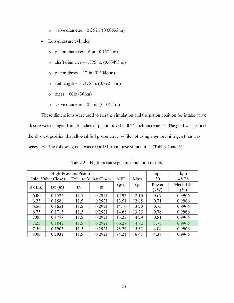
These dimensions were used to run the simulation and the piston position for intake valve
closure was changed from 6 inches of piston travel in 0.25-inch increments. The goal was to find
the shortest position that allowed full piston travel while not using anymore nitrogen than was
necessary. The following data was recorded from those simulations (Tables 2 and 3):
Table 2 – High-pressure piston simulation results.
High-Pressure Piston MFR (g/s)
Mass (g)
mph kph Inlet Valve Closes Exhaust Valve Closes 30 48.28
Bx (in.) Bx (m) In. m Power (kW)
Mech Eff. (%)
6.00 0.1524 11.5 0.2921 12.92 12.10 0.67 0.9966 6.25 0.1588 11.5 0.2921 13.51 12.65 0.71 0.9966 6.50 0.1651 11.5 0.2921 14.10 13.20 0.75 0.9966 6.75 0.1715 11.5 0.2921 14.68 13.75 0.78 0.9966 7.00 0.1778 11.5 0.2921 15.25 14.29 0.81 0.9966 7.25 0.1842 11.5 0.2921 66.28 14.82 3.77 0.9966 7.50 0.1905 11.5 0.2921 73.26 15.35 4.04 0.9966 8.00 0.2032 11.5 0.2921 84.21 16.43 4.38 0.9966
25

Table 3 – Low-pressure piston simulation results.
Low-Pressure Piston MFR (g/s)
Mass (g)
mph kph Inlet Valve Closes Exhaust Valve Closes 30 48.28032
Bx (in.) Bx (m) In. m Power (kW)
Mech Eff. (%)
6 0.1524 11.5 0.2921 11.15 10.45 0.7316 0.9954 6.25 0.15875 11.5 0.2921 11.885 11.135 0.77255 0.9954 6.5 0.1651 11.5 0.2921 12.62 11.82 0.8135 0.9954 6.75 0.17145 11.5 0.2921 13.355 12.505 0.85445 0.9954
7 0.1778 11.5 0.2921 47.35 13.54 2.954 0.9954
This flow rate data was used at the required pressures for analyzing the flow circuit for
each piston. Summations of all minor losses throughout each flow circuit were performed (Table
4). The following results for those calculations were recorded:
Table 4 - Summation of all minor losses in each flow circuit.
MFR (g/s) Inlet Pressure (psi)
Outlet Pressure (psi)
Pressure Drop (psi)
Change (%)
High 66.28 548.4 500 48.4 8.83 Low 47.35 106.3 100 6.3 5.93
26

CHAPTER 5
RESULTS AND ANALYSIS
The simulation results for the high-pressure piston show that under the required load, the
intake valve must stay open through the first 7.25 inches of piston travel to achieve a full piston
stroke and the necessary velocity (Table 2). Achieving a full piston stroke requires an MFR of
66.28 g/s or 0.06628 kg/sec. The high-pressure piston achieves a mechanical efficiency of
0.9966 or 99.66% for the piston alone.
The results for the low-pressure piston show that under the required load, the intake valve
must stay open through the first 7.0 inches of piston travel to achieve a full piston stroke and the
necessary velocity (Table 3). This requires an MFR of 47.35 g/s or 0.04735 kg/sec. The low-
pressure piston achieves a mechanical efficiency of 0.9954 or 99.54%.
The piston simulation results are based on a constant load, so that the same amount of
force is necessary for each piston motion. Under this constant load, if the intake valve closes
before the piston travels 7 or 7.25 inches (high pressure and low pressure, respectively), the
piston will not achieve a full stroke.
The flow circuit analysis of the high-pressure flow circuit shows that to achieve an outlet
pressure of 500 psi at 66.28 g/s requires an initial pressure of 548.4 psi, which is an 8.83% loss
through the circuit, an efficiency of 91.17%. The largest single point of pressure loss was due to
the 36.1-psi drop at the control valve (Fig. 12) because a valve ¼-inch diameter was used in
comparison to the rest of the flow circuit (½-inch diameter). A control valve with a larger
diameter would reduce the amount of pressure loss, but the high-pressure piston only allows for
valves of up to ⅜-inch diameter (Fig. 13).
27

Fig. 12 – High-pressure solenoid valve.
Fig. 13 – High-pressure drive assembly.
28

The flow circuit analysis of the low-pressure flow circuit shows that to achieve an outlet
pressure of 100 psi at 47.35 g/s requires an initial pressure of 106.3 psi which is a 5.93% loss
through the circuit, an efficiency of 94.07%. There were no significant losses of pressure at any
particular point of this flow circuit (Fig. 14 and 15).
Fig. 14 – Low-pressure solenoid valve.
Fig. 15 – Low-pressure drive assembly.
29

The flow circuit analysis was performed with one control valve open and the other
control valve closed, just like in normal operation. The analysis was performed with no
consideration for elevation change because any elevation change would be negligible.
30

CHAPTER 6
SUMMARY, CONCLUSIONS, AND RECOMMENDATIONS
Summary of the Study
The purpose of this study was to perform a mechanical efficiency analysis of a dual,
double-acting piston nitrogen propulsion system. This study focused on the two main
components of this system, the driving pistons and the flow circuits to power those pistons.
The double-acting pistons were simulated to achieve their full piston stroke while using
the least amount of nitrogen necessary. The pistons would prove themselves to be highly
efficient with proper valve timing that is adaptive to the load. The study also shows the
difference in power of each piston at its respective pressure.
The flow circuit analysis shows that both flow circuits can adequately handle the pressure
and flow requirements that the pistons require. The analysis also showed that the control valves
on the high-pressure circuit are not ideal for this application (Fig. 12). The large decrease in
diameter at the valve, ½ inch down to ¼ inch, increased the pressure loss. The piston valve ports
allow for a valve up to a ⅜ inch in diameter and could possibly be drilled larger, but no other
valve was available at the time that operated on a 12-volt system, and that could handle the
pressure requirements. Development of larger-diameter high-pressure valves appears to be a
necessary enabling technology worthy of research based on these results.
Answer to the Research Questions
1. Is the ηII (mechanical efficiency) of each piston at least 90%?
The two pistons were analyzed with a MATLAB Simulink computer simulation of a
pneumatic engine operation using a double-acting piston [2]. Inputs included the mass of the
31

piston and all moving parts (piston, rod, rack, gear, etc.), useful areas of each cavity, input and
output pressures, and required piston velocity.
Null: The ηII (mechanical efficiency) for each piston is equal to or greater than 90%.
HO2: ηII Piston ≥ 90%
Alternative: The mechanical efficiency for each piston is less than 90%.
HA2: ηII Piston < 90%
Answer: The results from the MATLAB Simulink computer simulation show that the
high-pressure and low-pressure pistons achieved ηII values of 99.66% and 99.54%, respectively.
These values are within the null hypothesis: therefore the answer is yes - the ηII of each piston is
at least 90%.
2. Will the pressure drops in the flow circuits (high-pressure and low-pressure) be more
than 10%, based on the MFR requirements of each piston?
Each flow circuit was analyzed by utilizing Design Flow Solutions DesignNet 4, NIST
(National Institute of Standards and Technology) Reference Fluid Thermodynamic and Transport
Properties data for nitrogen, and MFRs calculated from the Simulink simulation.
Null: The pressure losses for each circuit are less than or equal to 10%.
HO1: PL Circuit ≤ 10%
Alternative: The pressure losses for each circuit are greater than 10%.
HA1: PL Circuit > 10%
Answer: The use of Design Flow Solutions DesignNet 4, NIST (National Institute of
Standards and Technology) Reference Fluid Thermodynamic and Transport Properties data for
nitrogen, and MFRs calculated from the Simulink simulation resulted in pressure losses of 8.83%
and 5.93% for the high-pressure and low-pressure flow circuits, respectively. These values are
32

within the null hypothesis: therefore, the answer is yes – pressure losses for each circuit are less
than or equal to 10% at 30 mph.
Conclusions
After analyzing this research study, the designers concluded that this dual double-acting
piston nitrogen propulsion system meets their intended goals. It would be beneficial to look for
alternative control valves for the high-pressure circuit that are less restrictive that the ones
currently implemented.
Strengths of the Study
The main strength of this study that it shows that there is a viable potential for cryogenic
heat engines. This study should help encourage future research into the potential use of
cryogenic heat engines for automotive applications.
Recommendations for Further Research
Further cryogenic heat engine research should continue in its current direction, working
to get the more work out of the potential that liquid nitrogen offers. The use of lighter materials
for these systems would also be beneficial. It would also be beneficial to develop future
simulations that allow variable loads and valve timing, to maximize efficiency at any piston
speed. More research to improve high-pressure valves would also be helpful.
33

APPENDIX
COMPONENTS AND FITTINGS TO BE ANALYZED WITH DESIGN FLOW SOLUTIONS
34

Liquid Nitrogen Tank – 45 gallon – 3/8 inch NPT female outlet
Solenoid Valve – 500 psi – 12 V – ½ inch NPT female inlet and outlet
Heat Exchanger (3) – 8 fin (4-inch fins) – 96-inch length – aluminum – ¾-inch NPT male
Pressure Relief Valve – 500 psi – ½-inch NPT male inlet
Pressure Switch – 500 psi – ¼-inch NPT male
Piston Control Valves (high pressure) (4) – 12 VDC – ¼-inch NPT female inlet and
outlet
High Pressure Piston – 500 psi – 12-inch stroke – 2.5-inch diameter, 3/8-inch NPT
female inlets and outlets
Heat Exchanger – circular fins (1½-inch diameter) – ½-inch copper type K tubing
Pressure Relief Valve – 100 psi – ½-inch NPT male inlet
Pressure Switch – 90 psi – 1/8-inch NPT male
Solenoid Valve – 100 psi – 12 V – ½-inch NPT female inlet and outlet
Low-Pressure Reservoir (2) – 4-inch diameter by 12-inch length – 1/8-inch NPT female
inlet
Piston Control Valves (4) – 12 VDC – ½-inch NPT female inlet and outlet
Low Pressure Piston – 100 psi – 12-inch stroke – 6-inch diameter – ½” NPT female inlets
and outlets
35

36
37

BIBLIOGRAPHY
Anderson, Blaine W. The Analysis and Design of Pneumatic Systems, John Wiley & Sons, Inc., Krieger Publishing Company, 2001. 1967.
Avallone, E. A. and T. Baumeister. Marks’ Standard Handbook for Mechanical Engineers. 11th
ed. New York: McGraw-Hill, Inc., 1997. Binder, R. C. Fluid Mechanics. Englewood Cliffs, NJ: Prentice-Hall, Inc., 1973. Calgaro, C., J. F. Coulombel, and Thierry Goudon. Analysis and Simulation of Fluid Dynamics.
Basel, France: Birkhauser Publishing, 2007. Çengel, Yunus A. and Michael A. Boles. Thermodynamics: An Engineering Approach. 4th ed.
New York: McGraw Hill, 2002. Colebrook, C. F. “Turbulent Flow in Pipes,” Journal of the Inst. Civil Eng. 11, p. 133, 1938. Crane Co. Engineering Division. “Flow of Fluids through Valves, Fittings, and Pipe.” Crane Co.
Technical Paper No. 410, Crane Co.; 21st printing, 1982. Kambe, T. Elementary Fluid Mechanics. Hackensack, N.J.: World Scientific Publishing, 2007. Koumoutsakos, P. and I. Mezic. Control of Fluid Flow. Berlin: Springer Publishing, 2006. Kudryavtsev, I. N., A. V. Kramskoy, A. I. Pyatak, and M. C. Plummer. “Computer Simulation of
Pneumatic Engine Operation,” International Scientific Journal for Alternative Energy and Ecology, 3(23), pp. 80-89, 2005.
Mott, Robert L. Applied Fluid Mechanics. 5th ed. Upper Saddle River, NJ: Prentice Hall, 2000. Narasimhan, S. A First Course in Fluid Mechanics. Boca Raton, FL: CRC Press, 2007. National Institute of Standards and Technology. NIST Reference Fluid Thermodynamic and
Transport Properties – REFPROP. Version 7.0. Gaithersburg, MD: U.S. Department of Commerce, 2002.
Ordonez, C. A. “Cryogenic Heat Engine,” American Journal of Physics 64: pp. 479-481, 1996. Ordonez, C. A. and M. C. Plummer. “Cold Thermal Storage and Cryogenic Heat Engines for
Energy Storage Applications,” Energy Sources 19: pp. 389-396, 1997. Ordonez, C. A. “Liquid Nitrogen Fueled, Closed Brayton Cycle Cryogenic Heat Engine,”
Energy Conversion and Management 41: pp. 331-341, 2000.
38

39
Plummer, M. C., C. P. Koehler, D. R. Flanders, R. F. Reidy, and C. A. Ordonez. “Cryogenic Heat Engine Experiment,” Advances in Cryogenic Engineering 43: pp. 1245-1252, 1998.
Plummer, M. C., C. A. Ordonez, and R. F. Reidy. “A Review of Liquid Nitrogen Propelled
Vehicle Programs in the United States of America,” Proceedings of the International Scientific Conference on Automobile Transport and Road Enterprises on the Threshold of the Third Millennium, Paper No. 629.1, pp. 47-52, 2000.
White, Frank M. Fluid Mechanics, 5th ed. New York: McGraw-Hill Higher Education, 1998.