design and control of automotive propulsion systems
TRANSCRIPT

6000 Broken Sound Parkway, NW Suite 300, Boca Raton, FL 33487711 Third Avenue New York, NY 100172 Park Square, Milton Park Abingdon, Oxon OX14 4RN, UK
an informa business
www.taylorandfrancisgroup.com
K11064
Better Understand the relationship Between powertrain system design and its Control integration
While powertrain system design and its control integration are traditionally divided into two different functional groups, a growing trend introduces the integration of more electronics (sensors, actuators, and controls) into the powertrain system. This has impacted the dynamics of the system, changing the traditional mechanical powertrain into a mechatronic powertrain, and creating new opportunities for improved efficiency. Design and Control of Automotive Propulsion Systems focuses on the ICE-based automotive powertrain system (while presenting the alternative powertrain systems where appropriate). Factoring in the multidisciplinary nature of the automotive propulsion system, this text does two things—adopts a holistic approach to the subject, especially focusing on the relationship between propulsion system design and its dynamics and electronic control, and covers all major propulsion system components, from internal combustion engines to transmissions and hybrid powertrains.
The book introduces the design, modeling, and control of the current automotive propulsion system, and addresses all three major subsystems: system level optimization over engines, transmissions, and hybrids (necessary for improving propulsion system efficiency and performance). It provides examples for developing control-oriented models for the engine, transmission, and hybrid. It presents the design principles for the powertrain and its key subsystems. It also includes tools for developing control systems and examples on integrating sensors, actuators, and electronic control to improve powertrain efficiency and performance. In addition, it presents analytical and experimental methods, explores recent achievements, and discusses future trends.
Comprised of five Chapters Containing the fUndamentals as well as new researCh, this text:
• Examines the design, modeling, and control of the internal combustion engine and its key subsystems:the valve actuation system, the fuel system, and the ignition system
• Expounds on the operating principles of the transmission system, the design of the clutch actuation system, and transmission dynamics and control
• Explores the hybrid powertrain, including the hybrid architecture analysis, the hybrid powertrain model, and the energy management strategies
• Explains the electronic control unit and its functionalities—the software-in-the-loop and hardware-in-the-loop techniques for developing and validating control systems
Design and Control of Automotive Propulsion Systems provides the background of the automotive propulsionsystem, highlights its challenges and opportunities, and shows the detailed procedures for calculating vehicle power demand and the associated powertrain operating conditions.
Automotive Engineering
D e s i g n a n d C o n t r o l o f AuTomoTIvE ProPulsIon sysTEms
Design and Control of AuTom
oTIvE Pro
PulsIon sysTEm
ssunZhu
CAT#K11064 cover.indd 1 11/17/14 12:24 AM


D e s i g n a n d C o n t r o l o f
A u t o m o t i v e P r o P u l s i o n s y s t e m s
MECHANICAL and AEROSPACE ENGINEERING Frank Kreith & Darrell W. Pepper
Series Editors
RECENTLY PUBLISHED TITLESAir Distribution in Buildings, Essam E. Khalil
Alternative Fuels for Transportation, Edited by Arumugam S. Ramadhas
Computer Techniques in Vibration, Edited by Clarence W. de Silva
Design and Control of Automotive Propulsion Systems, Zongxuan Sun and Guoming G. Zhu
Distributed Generation: The Power Paradigm for the New Millennium, Edited by Anne-Marie Borbely and Jan F. Kreider
Elastic Waves in Composite Media and Structures: With Applications to Ultrasonic Nondestructive Evaluation, Subhendu K. Datta and Arvind H. Shah
Elastoplasticity Theory, Vlado A. Lubarda
Energy Audit of Building Systems: An Engineering Approach, Moncef Krarti
Energy Conversion, Second Edition, Edited by D. Yogi Goswami and Frank Kreith
Energy Efficiency in the Urban Environment, Heba Allah Essam E. Khalil and Essam E. Khalil
Energy Management and Conservation Handbook, Second Edition, Edited by Frank Kreith and D. Yogi Goswami
Essentials of Mechanical Stress Analysis, Amir Javidinejad
The Finite Element Method Using MATLAB®, Second Edition, Young W. Kwon and Hyochoong Bang
Fluid Power Circuits and Controls: Fundamentals and Applications, John S. Cundiff
Fuel Cells: Principles, Design, and Analysis, Shripad Revankar and Pradip Majumdar
Fundamentals of Environmental Discharge Modeling, Lorin R. Davis
Handbook of Energy Efficiency and Renewable Energy, Edited by Frank Kreith and D. Yogi Goswami
Handbook of Hydrogen Energy, Edited by S.A. Sherif, D. Yogi Goswami, Elias K. Stefanakos, and Aldo Steinfeld
Heat Transfer in Single and Multiphase Systems, Greg F. Naterer
Heating and Cooling of Buildings: Design for Efficiency, Revised Second Edition, Jan F. Kreider, Peter S. Curtiss, and Ari Rabl
Intelligent Transportation Systems: Smart and Green Infrastructure Design, Second Edition, Sumit Ghosh and Tony S. Lee
Introduction to Biofuels, David M. Mousdale
Introduction to Precision Machine Design and Error Assessment, Edited by Samir Mekid
Introductory Finite Element Method, Chandrakant S. Desai and Tribikram Kundu
Large Energy Storage Systems Handbook, Edited by Frank S. Barnes and Jonah G. Levine

Machine Elements: Life and Design, Boris M. Klebanov, David M. Barlam, and Frederic E. Nystrom
Mathematical and Physical Modeling of Materials Processing Operations, Olusegun Johnson Ilegbusi, Manabu Iguchi, and Walter E. Wahnsiedler
Mechanics of Composite Materials, Autar K. Kaw
Mechanics of Fatigue, Vladimir V. Bolotin
Mechanism Design: Enumeration of Kinematic Structures According to Function, Lung-Wen Tsai
Mechatronic Systems: Devices, Design, Control, Operation and Monitoring, Edited by Clarence W. de Silva
The MEMS Handbook, Second Edition (3 volumes), Edited by Mohamed Gad-el-Hak
MEMS: Introduction and Fundamentals
MEMS: Applications
MEMS: Design and Fabrication
Multiphase Flow Handbook, Edited by Clayton T. Crowe
Nanotechnology: Understanding Small Systems, Third Edition, Ben Rogers, Jesse Adams, Sumita Pennathur
Nuclear Engineering Handbook, Edited by Kenneth D. Kok
Optomechatronics: Fusion of Optical and Mechatronic Engineering, Hyungsuck Cho
Practical Inverse Analysis in Engineering, David M. Trujillo and Henry R. Busby
Pressure Vessels: Design and Practice, Somnath Chattopadhyay
Principles of Solid Mechanics, Rowland Richards, Jr.
Principles of Sustainable Energy Systems, Second Edition, Edited by Frank Kreith with Susan Krumdieck, Co-Editor
Thermodynamics for Engineers, Kau-Fui Vincent Wong
Vibration and Shock Handbook, Edited by Clarence W. de Silva
Vibration Damping, Control, and Design, Edited by Clarence W. de Silva
Viscoelastic Solids, Roderic S. Lakes
Weatherization and Energy Efficiency Improvement for Existing Homes: An Engineering Approach, Moncef Krarti

Boca Raton London New York
CRC Press is an imprint of theTaylor & Francis Group, an informa business
D e s i g n a n d C o n t r o l o f
A u t o m o t i v e P r o P u l s i o n s y s t e m sZ o n g x u A n s u ng u o m i n g g . Z h u

CRC PressTaylor & Francis Group6000 Broken Sound Parkway NW, Suite 300Boca Raton, FL 33487-2742
© 2015 by Taylor & Francis Group, LLCCRC Press is an imprint of Taylor & Francis Group, an Informa business
No claim to original U.S. Government worksVersion Date: 20140718
International Standard Book Number-13: 978-1-4398-2019-3 (eBook - PDF)
This book contains information obtained from authentic and highly regarded sources. Reasonable efforts have been made to publish reliable data and information, but the author and publisher cannot assume responsibility for the valid-ity of all materials or the consequences of their use. The authors and publishers have attempted to trace the copyright holders of all material reproduced in this publication and apologize to copyright holders if permission to publish in this form has not been obtained. If any copyright material has not been acknowledged please write and let us know so we may rectify in any future reprint.
Except as permitted under U.S. Copyright Law, no part of this book may be reprinted, reproduced, transmitted, or uti-lized in any form by any electronic, mechanical, or other means, now known or hereafter invented, including photocopy-ing, microfilming, and recording, or in any information storage or retrieval system, without written permission from the publishers.
For permission to photocopy or use material electronically from this work, please access www.copyright.com (http://www.copyright.com/) or contact the Copyright Clearance Center, Inc. (CCC), 222 Rosewood Drive, Danvers, MA 01923, 978-750-8400. CCC is a not-for-profit organization that provides licenses and registration for a variety of users. For organizations that have been granted a photocopy license by the CCC, a separate system of payment has been arranged.
Trademark Notice: Product or corporate names may be trademarks or registered trademarks, and are used only for identification and explanation without intent to infringe.
Visit the Taylor & Francis Web site athttp://www.taylorandfrancis.com
and the CRC Press Web site athttp://www.crcpress.com
vii
Contents
Preface ..............................................................................................................................................xiAbout the Authors ...................................................................................................................... xiii
1. Introduction of the Automotive Propulsion System .......................................................11.1 Background of the Automotive Propulsion System .................................................1
1.1.1 Historic Perspective .........................................................................................11.1.2 Current Status and Challenges ......................................................................11.1.3 Future Perspective ...........................................................................................2
1.2 Main Components of the Automotive Propulsion System .....................................31.3 Vehicle Power Demand Analysis ................................................................................3
1.3.1 Calculation of Vehicle Tractive Force ............................................................41.3.1.1 Traction Limit ...................................................................................61.3.1.2 Maximum Acceleration Limit ........................................................61.3.1.3 Maximum Grade Limit....................................................................61.3.1.4 Vehicle Power Demand ...................................................................71.3.1.5 Vehicle Performance Envelope .......................................................81.3.1.6 Vehicle Power Envelope ..................................................................8
1.3.2 Vehicle Power Demand during Driving Cycles ..........................................9References ............................................................................................................................... 11
2. Design, Modeling, and Control of Internal Combustion Engine .............................. 132.1 Introduction to Engine Subsystems ......................................................................... 132.2 Mean Value Engine Model......................................................................................... 14
2.2.1 Mean Value Gas Flow Model ....................................................................... 142.2.1.1 Valve Dynamic Model ................................................................... 152.2.1.2 Manifold Filling Dynamic Model ................................................ 152.2.1.3 Turbine and Compressor Models................................................. 15
2.2.2 Crank-Based One-Zone SI Combustion Model ......................................... 172.2.2.1 Crank-Based Methodology ........................................................... 172.2.2.2 Gas Exchange Process Modeling ................................................. 182.2.2.3 One-Zone SI Combustion Model ................................................. 20
2.2.3 Combustion Event-Based Dynamic Model ................................................ 212.2.3.1 Fueling Dynamics and Air-to-Fuel Ratio Calculation .............. 212.2.3.2 Engine Torque and Crankshaft Dynamic Model ......................22
2.3 Valve Actuation System ..............................................................................................232.3.1 Valve Actuator Design ..................................................................................23
2.3.1.1 Challenges for Developing FFVA Systems ................................. 242.3.1.2 System Design .................................................................................25
2.3.2 Valve Actuator Model and Control ............................................................. 262.3.2.1 System Hardware and Dynamic Model .....................................282.3.2.2 Robust Repetitive Control Design ...............................................332.3.2.3 Experimental Results .....................................................................36
viii Contents
2.4 Fuel Injection Systems ................................................................................................402.4.1 Fuel Injector Design and Optimization ......................................................40
2.4.1.1 PFI Fuel System ............................................................................... 412.4.1.2 DI Fuel System ................................................................................ 41
2.4.2 Fuel Injector Model and Control..................................................................462.5 Ignition System Design and Control ........................................................................ 47
2.5.1 Ignition System ...............................................................................................502.5.2 MBT Timing Detection and Its Closed-Loop Control ..............................50
2.5.2.1 Full-Range MBT Timing Detection ............................................. 512.5.2.2 Closed-Loop MBT Timing Control ..............................................54
2.5.3 Stochastic Ignition Limit Estimation and Control ....................................552.5.3.1 Stochastic Ignition Limit Estimation ...........................................552.5.3.2 Knock Intensity Calculation and Its Stochastic Properties ......562.5.3.3 Stochastic Limit Control ................................................................58
2.5.4 Experimental Study Results ......................................................................... 612.5.4.1 Closed-Loop MBT Timing Control .............................................. 612.5.4.2 Closed-Loop Retard Limit Control ..............................................652.5.4.3 Closed-Loop Knock Limit Control .............................................. 67
References ............................................................................................................................... 70
3. Design, Modeling, and Control of Automotive Transmission Systems ...................753.1 Introduction to Various Transmission Systems ...................................................... 753.2 Gear Ratio Realization for Automatic Transmission ............................................. 76
3.2.1 Planetary Gear Set ......................................................................................... 763.2.2 Speed and Torque Calculation for Automatic Transmission................... 783.2.3 Speed and Torque Calculation during Gear Shifting ...............................83
3.3 Design and Control of Transmission Clutches ....................................................... 873.3.1 Clutch Design ................................................................................................. 873.3.2 New Clutch Actuation Mechanism .............................................................88
3.3.2.1 Simulation and Experimental Results ......................................... 913.3.3 Feedforward Control for Clutch Fill ........................................................... 93
3.3.3.1 Clutch System Modeling ............................................................... 943.3.3.2 Formulation of the Clutch Fill Control Problem ........................ 963.3.3.3 Optimal Control Design ................................................................ 983.3.3.4 Simulation and Experimental Results ....................................... 103
3.3.4 Pressure-Based Clutch Feedback Control ................................................ 1093.3.4.1 System Dynamics Modeling ....................................................... 1113.3.4.2 Robust Nonlinear Controller and Observer Design ............... 115
3.4 Driveline Dynamics and Control ........................................................................... 123References ............................................................................................................................. 126
4. Design, Modeling, and Control of Hybrid Systems .................................................... 1294.1 Introduction to Hybrid Vehicles ............................................................................. 129
4.1.1 Various Types of Hybrid Vehicles ............................................................. 1294.2 Hybrid Architecture Analysis ................................................................................. 130
4.2.1 Parallel Hybrid Architecture ...................................................................... 1304.2.2 Series Hybrid Architecture ........................................................................ 1314.2.3 Power-Split Hybrid Architecture ............................................................... 132
ixContents
4.3 Hybrid System Dynamics and Control .................................................................. 1334.3.1 Dynamic Models for Hybrid System ........................................................ 1334.3.2 Hybrid System Control ............................................................................... 135
4.3.2.1 Transient Emission and Fuel Efficiency Optimal Control ..... 1354.3.2.2 DP-Based Extremum Seeking Energy Management
Strategy ..........................................................................................1574.3.2.3 Driveline Dynamics Control for Hybrid Vehicles ................... 164
References ............................................................................................................................. 167
5. Control System Integration and Implementation ........................................................ 1695.1 Introduction to the Electronic Control Unit .......................................................... 169
5.1.1 Electronic Control Unit (ECU) ................................................................... 1695.1.1.1 ECU Control Features .................................................................. 169
5.1.2 Communications between ECUs ............................................................... 1725.1.3 Calibration Methods for ECU .................................................................... 173
5.2 Control Software Development .............................................................................. 1745.2.1 Control Software Development Process ................................................... 1745.2.2 Automatic Code Generation ....................................................................... 1765.2.3 Software-in-the-Loop (SIL) Simulation ..................................................... 1765.2.4 Hardware-in-the-Loop (HIL) Simulation ................................................. 177
5.2.4.1 HCCI Combustion Background ................................................. 1775.2.4.2 Multistep Combustion Mode Transition Strategy ................... 1795.2.4.3 Air-to-Fuel Ratio Tracking Problem .......................................... 1825.2.4.4 Engine Air Charge Dynamic Model ......................................... 1845.2.4.5 LQ Tracking Control Design ...................................................... 1855.2.4.6 CIL Simulation Results and Discussion .................................... 187
5.3 Control System Calibration and Integration ......................................................... 188References ............................................................................................................................. 190


xi
Preface
Transportation consumes about 30% of the total energy in the United States. In many emerging markets around the world, transportation, especially personal transportation, has been growing at a rapid pace. Consequently, energy consumption and its environmen-tal impact are now among the most challenging problems humans face. From a technical perspective, construction machinery and agriculture equipment share similar challenges, as all mobile applications have to carry energy onboard and convert energy into mechani-cal motion in real time to meet the demand of the specific function. The objective of this book is to present the design and control of automotive propulsion systems in order to promote innovations in transportation and mobile applications, and therefore reduce their energy consumption and emissions.
There are two unique features of this book. One is that given the multidisciplinary nature of the automotive propulsion system, we adopt a holistic approach to present the subject, especially focusing on the relationship between propulsion system design and its dynamics and electronic control. A critical trend in this area is to have more electronics, including sensors, actuators, and controls, integrated into the powertrain system. This is going to change the traditional mechanical powertrain into a mechatronic powertrain. Such change will have profound impact on the complex dynamics of the powertrain system and create new opportunities for improving system efficiency. The other is that we cover all major propulsion system components, from internal combustion engines to transmissions and hybrid powertrains. Given the trend of vehicle development, system-level optimization over engines, transmissions, and hybrids is necessary for improving propulsion system efficiency and performance. We treat all three major subsystems in the book.
Chapter 1 presents the background of the automotive propulsion system, highlights its challenges and opportunities, and shows the detailed procedures for calculating vehicle power demand and the associated powertrain operating conditions. Chapter 2 presents the design, modeling, and control of the internal combustion engine and its key subsystems: the valve actuation system, the fuel system, and the ignition system. Chapter 3 presents the operating principles of the transmission system, the design of the clutch actu-ation system, and transmission dynamics and control. Chapter 4 presents the hybrid pow-ertrain, including the hybrid architecture analysis, the hybrid powertrain model, and the energy management strategies. Chapter 5 presents the electronic control unit and its func-tionalities, the software-in-the-loop and hardware-in-the-loop techniques for developing and validating control systems.
This book is intended for both engineering students and automotive engineers and researchers who are interested in designing the automotive propulsion system, optimiz-ing its dynamic behavior, and control system integration and optimization. For the engi-neering students, this book can be used as a textbook for a senior technical elective class or a graduate-level class. Similar content has been taught in a graduate-level class at the University of Minnesota and received very positive feedback from students. For auto-motive engineers, the book can be used to better understand the relationship between powertrain system design and its control integration, which is traditionally divided into two different functional groups in the automotive industry. It will also help automotive

xii Preface
engineers to understand advanced control methodologies and their implementation, and facilitate the introduction of new design and control technologies into future automobiles.
We thank and acknowledge our graduate students for their contributions to the research work represented in the book. We especially want to thank Yaoying Wang, Yu Wang, Xingyong Song, and Xiaojian Yang for their help with editing and proofreading of the book.
Zongxuan Sun and Guoming Zhu

xiii
About the Authors
Dr. Zongxuan Sun is currently an associate professor of mechanical engineering at the University of Minnesota, Minneapolis. He was a staff researcher from 2006 to 2007 and a senior researcher from 2000 to 2006 at the General Motors Research and Development Center, Warren, Michigan. Dr. Sun received his BS degree in automatic control from Southeast University, Nanjing, China, in 1995, and the MS and PhD degrees in mechani-cal engineering from the University of Illinois at Urbana-Champaign, in 1998 and 2000, respectively. He has published more than 90 refereed technical papers and received 19 U.S. patents. His current research interests include controls and mechatronics with applica-tions to the automotive propulsion systems. Dr. Sun is a recipient of the George W. Taylor Career Development Award from the College of Science and Engineering, University of Minnesota, the National Science Foundation CAREER Award, the SAE Ralph R. Teetor Educational Award, the Best Paper Award from the 2012 International Conference on Advanced Vehicle Technologies and Integration, the Inventor Milestone Award, the Spark Plug Award, and the Charles L. McCuen Special Achievement Award from GM Research and Development.
Dr. Guoming G. Zhu is a professor of mechanical engineering and electrical/ computer engineering at Michigan State University. Prior to joining the ME and ECE departments, he was a technical fellow in advanced powertrain systems at Visteon Corporation. He also worked for Cummins Engine Co. as a technical advisor. Dr. Zhu earned his PhD (1992) in aerospace engineering at Purdue University. His BS and MS degrees (1982 and 1984, respectively) were from Beijing University of Aeronautics and Astronautics in China. His current research interests include closed-loop combustion control, adaptive control, closed-loop system identification, linear parameter varying (LPV) control of automotive systems, hybrid powertrain control and optimization, and thermoelectric generator man-agement systems. Dr. Zhu has more than 30 years of experience related to control theory and applications. He has authored or coauthored more than 140 refereed technical papers and received 40 U.S. patents. He was an associate editor for ASME Journal of Dynamic Systems, Measurement, and Control and a member of the editorial board of International Journal of Powertrain. Dr. Zhu is a fellow of the Society of Automotive Engineers (SAE) and American Society of Mechanical Engineers (ASME).


1
1Introduction of the Automotive Propulsion System
1.1 Background of the Automotive Propulsion System
1.1.1 Historic Perspective
Throughout human history, transportation of people and goods has always been a critical part of society. For a very long time (until the 19th century), this was accomplished by either human- or animal-driven vehicles. The steam engine fundamentally changed the transportation system, mainly by powering boats and trains with some applications for automobiles. At the end of the 19th century, the invention of the internal combustion engine (ICE) led to a complete revolution of both personal and commercial transportation. Over the past 100 years, the ICE has dominated the automotive propulsion system. This is mainly due to the energy density of the liquid fuel and the power density of the ICE. For the first time in human history, the ICE enables the controlled extraction of chemical energy in hydrocarbon fuels into mechanical motion through cyclic exothermic chemical reactions with high power density.
Tremendous improvement has been achieved for optimizing engine performance, efficiency, and emissions. Today’s ICE is a much more complex machine than its ancestor of a century ago. New technologies appear in nearly every subsystem of the ICE: air intake and exhaust system, fuel delivery and injection system, ignition system, cooling system, lubrication system, aftertreatment system, materials and manufacturing technology, and sensing and control system. This is the result of century-long efforts of continuous innova-tions involving science, engineering, and technology. The hallmark of such innovations is their multidisciplinary nature. This involves mechanical engineering, electrical engineer-ing, chemistry and materials, etc. If we zoom into the specific disciplines, they include thermodynamics, fluid mechanics, heat transfer, chemical reaction, design and manufac-turing, controls, etc. This multidisciplinary nature has served us well, but it also reveals the difficulties and complexities we will face as the technology evolves going forward.
1.1.2 Current Status and Challenges
As we entered the 21st century, new challenges emerged for the transportation system. On the one hand, it became an integral part of society. Both personal and commercial trans-portation through on-road vehicles became necessary tools for everyday life and economic activities. Off-road vehicles such as construction machinery and agriculture equipment also experienced significant growth for improving productivity in many industries and farming. On the other hand, the growing number of vehicles around the world poses a serious challenge to the sustainability of transportation and its impact on the environment.
2 Design and Control of Automotive Propulsion Systems
There are about 850 million automobiles in the world today, with a projected number of 2.5 billion by year 2050. These enormous numbers once again bring up a question that was debated more than a hundred years ago: What is the best propulsion system for automo-biles, and what are the energy sources that can sustain transportation? To answer such questions, research work for improving the efficiency of the ICE-based propulsion system, designing alternative propulsion systems, and developing renewable energies is being pursued. A good example is the emergence of hybrid vehicles more than 10 years ago. The hybrid powertrain is the first major change from the conventional powertrain by add-ing alternative power sources such as electrical power or fluid power to the system. More technical innovations are expected in the coming years that could reinvent the automotive propulsion system. To facilitate such innovations, this book is targeted to introducing the design, modeling, and control of the current automotive propulsion system, as well as presenting and discussing future trends.
1.1.3 Future Perspective
There have been numerous predictions and debates on the time when fossil fuel will be exhausted. Likely this is still a subject for debate even today. However, what is clear and less controversial is that global energy consumption has been growing at an unprecedented pace, conventional oil and gas supplies are being depleted, and there are tremendous concerns regarding the environmental impact of greenhouse gas emissions. To account for these challenges, three types of energy sources have been proposed for transporta-tion: liquid and gaseous fuels from both fossil and renewable sources, electricity, and hydrogen. The corresponding powertrain systems are internal combustion engine, electric propulsion, and fuel cell. While there are several discussions on the advantages and disad-vantages of different powertrain systems, their fate, to a large extent, will be determined by the competition among the various energy sources.
The main advantages of liquid fuels are the energy density, ease of handling, and trans-portation. So far, liquid fuels still have a clear advantage (order of magnitude) over any other energy sources for the ability to store energy per unit volume or weight. It is also fairly easy to replenish the fuel once it is consumed. The current practice of pumping gasoline at the gas station is in fact adding several hundred megajoules per minute into the vehicle. The extensive network of gas stations makes fuel transportation and storage con-venient and cost-effective. Those seemingly obvious features (energy density, easy to refuel and transport) are indeed the key factors that are needed for transportation energy supply. Using electricity as the fuel for transportation has the advantage of centralized emissions control since the emissions occur at the power plant rather than at the individual vehicle. It is also more versatile to incorporate renewable sources such as wind and solar energy. The main challenge for using electricity for transportation or mobile applications is the battery. To be competitive at large-scale deployment, the battery needs to have energy density that is comparable with the liquid fuel and easy and fast to recharge. The hydro-gen fuel uses the most abundant element in the world and produces no emissions at the vehicle level. However, production of the hydrogen fuel, as well as its transportation and storage, still faces many technical challenges. Although there are many studies for com-paring the well-to-wheel energy consumption of the different energy sources, this is not the focus of this book. Given the fact that liquid fuel will likely still dominate the energy supply for transportation for the foreseeable future, this book will focus on the ICE-based automotive powertrain system while presenting the alternative powertrain systems where appropriate.
3Introduction of the Automotive Propulsion System
1.2 Main Components of the Automotive Propulsion System
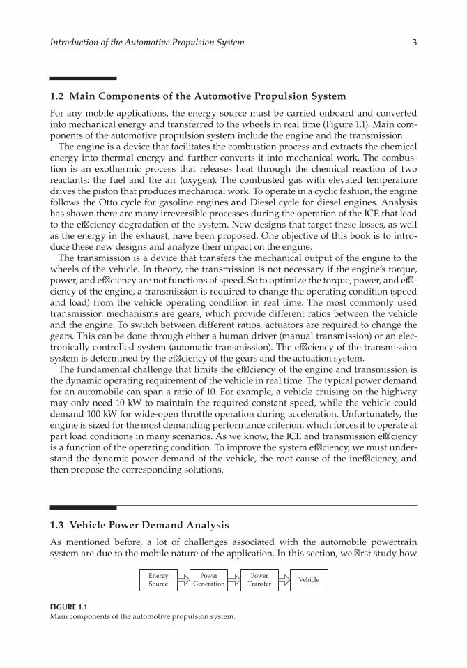
For any mobile applications, the energy source must be carried onboard and converted into mechanical energy and transferred to the wheels in real time (Figure 1.1). Main com-ponents of the automotive propulsion system include the engine and the transmission.
The engine is a device that facilitates the combustion process and extracts the chemical energy into thermal energy and further converts it into mechanical work. The combus-tion is an exothermic process that releases heat through the chemical reaction of two reactants: the fuel and the air (oxygen). The combusted gas with elevated temperature drives the piston that produces mechanical work. To operate in a cyclic fashion, the engine follows the Otto cycle for gasoline engines and Diesel cycle for diesel engines. Analysis has shown there are many irreversible processes during the operation of the ICE that lead to the efficiency degradation of the system. New designs that target these losses, as well as the energy in the exhaust, have been proposed. One objective of this book is to intro-duce these new designs and analyze their impact on the engine.
The transmission is a device that transfers the mechanical output of the engine to the wheels of the vehicle. In theory, the transmission is not necessary if the engine’s torque, power, and efficiency are not functions of speed. So to optimize the torque, power, and effi-ciency of the engine, a transmission is required to change the operating condition (speed and load) from the vehicle operating condition in real time. The most commonly used transmission mechanisms are gears, which provide different ratios between the vehicle and the engine. To switch between different ratios, actuators are required to change the gears. This can be done through either a human driver (manual transmission) or an elec-tronically controlled system (automatic transmission). The efficiency of the transmission system is determined by the efficiency of the gears and the actuation system.
The fundamental challenge that limits the efficiency of the engine and transmission is the dynamic operating requirement of the vehicle in real time. The typical power demand for an automobile can span a ratio of 10. For example, a vehicle cruising on the highway may only need 10 kW to maintain the required constant speed, while the vehicle could demand 100 kW for wide-open throttle operation during acceleration. Unfortunately, the engine is sized for the most demanding performance criterion, which forces it to operate at part load conditions in many scenarios. As we know, the ICE and transmission efficiency is a function of the operating condition. To improve the system efficiency, we must under-stand the dynamic power demand of the vehicle, the root cause of the inefficiency, and then propose the corresponding solutions.
1.3 Vehicle Power Demand Analysis
As mentioned before, a lot of challenges associated with the automobile powertrain system are due to the mobile nature of the application. In this section, we first study how
EnergySource
PowerGeneration
PowerTransfer Vehicle
FIGURE 1.1Main components of the automotive propulsion system.

4 Design and Control of Automotive Propulsion Systems
to calculate the vehicle tractive force, and then use it to analyze the vehicle power demand during various driving operations [1–3].
1.3.1 Calculation of Vehicle Tractive Force
For an automobile in motion, the typical resistance forces include rolling resistance due to tire and road interaction, wind resistance due to air and vehicle interaction, grade resis-tance due to the various grades of the road, and acceleration resistance due to the need to accelerate the vehicle mass.
As shown in Figure 1.2, the total tractive force for the vehicle is
FT = FR + FW + FG + FA (1.1)
where FT is the total tractive force at wheels (N), FR is the rolling resistance force (N), FW is the wind resistance force (N), FG is the grade resistance force (N), and FA is the acceleration resistance force (N).
We first show how to calculate the resistance forces and then use them to calculate the vehicle performance limit.
The rolling resistance force is
FR = KR · W · cos(θ) (1.2)
where KR is the rolling resistance coefficient (for typical values, see Table 1.1), W is the vehicle weight (N), and Θ is the road grade angle (radian).
The wind resistance force is
FW = KW · A · V 2 (1.3)
Wind
RollingResistance
θ
FIGURE 1.2Vehicle resistance forces.
TABLE 1.1
Typical Values for the Rolling Resistance Coefficient
KR Road Condition
0.01 Good paved roads0.015 Average paved roads0.02~0.025 Good gravel or soil0.1~0.15 Sand

5Introduction of the Automotive Propulsion System
where KW is the wind resistance coefficient (N/(m2/s)2), A is the vehicle frontal area (m2), and V is the vehicle speed (m/s) (Table 1.2).
The grade resistance force is
FG = W · sin(θ) (1.4)
where W and θ are the same as defined before.The acceleration resistance force is
FWg
a Wag
A = = (1.5)
where W is the same as defined before, a is the vehicle acceleration (m/s2), and g is the gravitational constant (9.8 N/kg).
When calculating the acceleration resistance force, if necessary, the equivalent vehicle weight that includes the effective weight of the powertrain rotating components can be used. This is because during vehicle acceleration, not only is the vehicle mass undergoing linear acceleration, but the rotational components of the powertrain system (engine iner-tia, transmission, drive shaft, and tire) are also undergoing angular acceleration, which is directly related to the linear acceleration of the vehicle. Depending on the inertia of the powertrain system relative to the vehicle mass, the equivalent vehicle weight could be significantly higher than the actual vehicle weight.
Now we are going to use the above equations to calculate the vehicle performance limit. What road grade will produce the same resistance force required for a given vehicle acceleration?
Let FG = FA; we have
sin( )W
W ag
⋅ θ =⋅
So
sin( )
ag
θ =
Using this equation, we can calculate the relationship between road grade angle and the acceleration, as shown in Table 1.3.
TABLE 1.2
Typical Values for Wind Resistance Coefficient
KW Vehicle Type
0.2995 Passenger cars0.4313 Small trucks0.599 Large trucks

6 Design and Control of Automotive Propulsion Systems
1.3.1.1 Traction Limit
The vehicle tractive force limit is based on the maximum traction available between tires and the road surface:
FT−Max = μ · W · X · cos(θ) (1.6)
where W and θ are the same as defined before, μ is the friction coefficient, and X is the percentage of vehicle weight on driving wheels (40%~60% for 2WD and 100% for 4WD).
1.3.1.2 Maximum Acceleration Limit
The maximum vehicle acceleration is determined by applying the maximum traction force to accelerate the vehicle without any grade resistance and wind resistance (vehicle speed at zero):
F F F W X K W W
ag
T Max R A R= + ⋅ ⋅ = ⋅ + ⋅−
Assume KR is very small and the vehicle is 4WD; we have
μ =
ag
So
aMax = μg (1.7)
1.3.1.3 Maximum Grade Limit
The maximum grade limit is determined by applying the maximum traction force to climb the grade without any acceleration and wind resistances (vehicle speed at zero):
FT = FR + FG ⇒ μ · W · X · cos(θ) = KR · W · cos(θ) + W · sin(θ)
Assume KR is very small and the vehicle is 4WD; we have
μcos(θ) = sin(θ) ⇒ tan(θ) = μ
TABLE 1.3
Vehicle Acceleration and Equivalent Road Grade Angle
Acceleration Equivalent Grade Angle (degree)
0 00.1 g 5.740.2 g 11.540.3 g 17.460.4 g 23.58
7Introduction of the Automotive Propulsion System
So
μ = 1.0 ⇒ θMax = 45° (1.8)
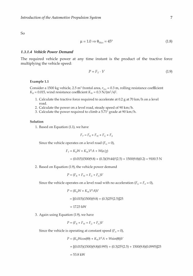
1.3.1.4 Vehicle Power Demand
The required vehicle power at any time instant is the product of the tractive force multiplying the vehicle speed:
P = FT · V (1.9)
Example 1.1
Consider a 1500 kg vehicle, 2.5 m2 frontal area, rtire = 0.3 m, rolling resistance coefficient KR = 0.015, wind resistance coefficient KW = 0.3 N/(m2/s)2.
1. Calculate the tractive force required to accelerate at 0.2 g at 70 km/h on a level road.
2. Calculate the power on a level road, steady speed of 90 km/h. 3. Calculate the power required to climb a 5.71° grade at 90 km/h.
Solution
1. Based on Equation (1.1), we have
FT = FR + FW + FG + FA
Since the vehicle operates on a level road (FG = 0),
FT = KRW + KWV2A + W(a/g)
= (0.015)1500(9.8) + (0.3)(19.44)2(2.5) + 1500(9.8)(0.2) = 9100.5 N
2. Based on Equation (1.9), the vehicle power demand
P = (FR + FW + FG + FA )V
Since the vehicle operates on a level road with no acceleration (FG = FA = 0),
P = (KRW + KWV2A)V
= [(0.015)(1500)(9.8) + (0.3)252(2.5)]25
= 17.23 kW
3. Again using Equation (1.9), we have
P = (FR + FW + FG + FA )V
Since the vehicle is operating at constant speed (FA = 0),
P = (KRWcos(Θ) + KWV2A + Wsin(θ))V
= [(0.015)(1500)(9.8)(0.995) + (0.3)252(2.5) + 1500(9.8)(0.0995)]25
= 53.8 kW
8 Design and Control of Automotive Propulsion Systems
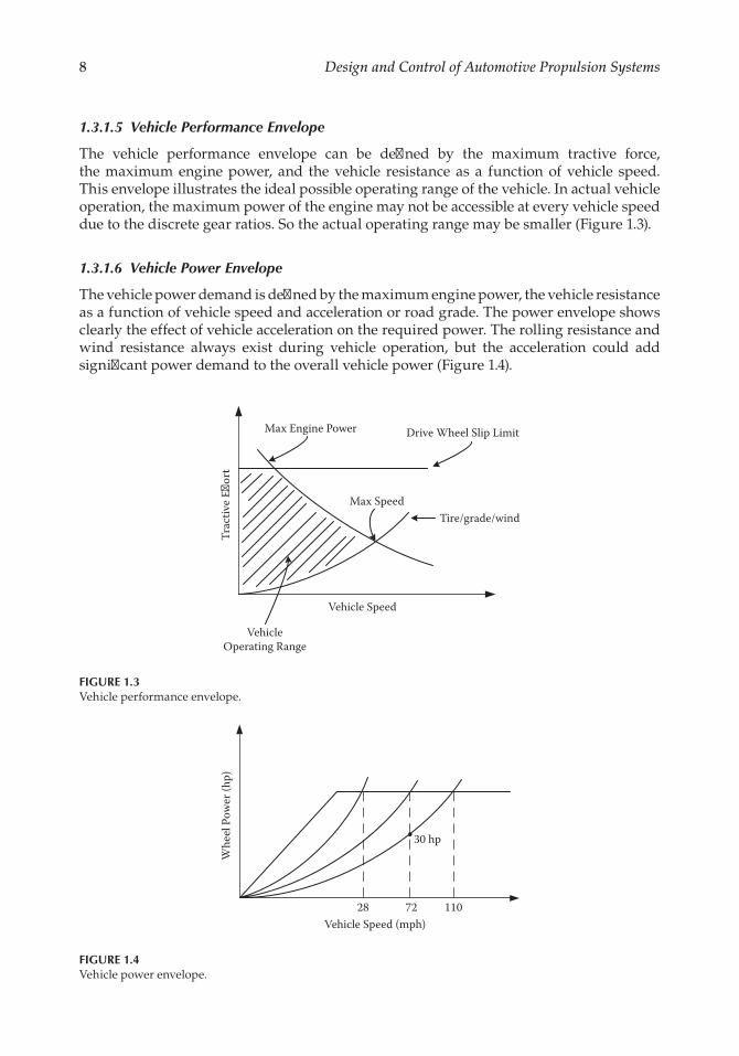
1.3.1.5 Vehicle Performance Envelope
The vehicle performance envelope can be defined by the maximum tractive force, the maximum engine power, and the vehicle resistance as a function of vehicle speed. This envelope illustrates the ideal possible operating range of the vehicle. In actual vehicle operation, the maximum power of the engine may not be accessible at every vehicle speed due to the discrete gear ratios. So the actual operating range may be smaller (Figure 1.3).
1.3.1.6 Vehicle Power Envelope
The vehicle power demand is defined by the maximum engine power, the vehicle resistance as a function of vehicle speed and acceleration or road grade. The power envelope shows clearly the effect of vehicle acceleration on the required power. The rolling resistance and wind resistance always exist during vehicle operation, but the acceleration could add significant power demand to the overall vehicle power (Figure 1.4).
Vehicle Speed
Tire/grade/windMax Speed
Drive Wheel Slip LimitMax Engine Power
Trac
tive E
�ort
VehicleOperating Range
FIGURE 1.3Vehicle performance envelope.
30 hp
Whe
el P
ower
(hp)
Vehicle Speed (mph)72 11028
FIGURE 1.4Vehicle power envelope.
9Introduction of the Automotive Propulsion System
1.3.2 Vehicle Power Demand during Driving Cycles
Based on the vehicle tractive force calculation, we can calculate the required power for propelling the vehicle for different driving cycles [4, 5]. The dynamic behavior in terms of both speed and power of the automobile sets the challenge for the powertrain system.
Example 1.2
Calculate the tractive effort and power demand for a given vehicle during the Federal Test Procedure (FTP) cycle (Table 1.4).
According to Equation (1.1), FT = KRW + KWV2A + W(a/g), once tractive force has been calculated, the operating point of the engine (speed ωe and torque/load Te) is calculated at each time step by using the following relationship:
r rr
V Tr
r rFe
f t
re
r
f tT, ω = =
As the FTP cycle begins at a vehicle speed of zero, the vehicle can be assumed to start in first gear at the first time step. These values are then fed into an engine map to determine the required percent throttle to produce the required engine torque at the required engine speed. This percent throttle, along with the vehicle speed, is fed into the transmission shift schedule for a typical automatic transmission with four forward speeds, which determines the shift command (upshift, downshift, or stay in current gear). Note that the percent throttle is calculated only for the purpose of determining gear shifts. This process is repeated at each time step, using the gear commanded in the previous time step to determine engine speed and torque, as well as the shift command for the current time step (which will be used in the next time step).
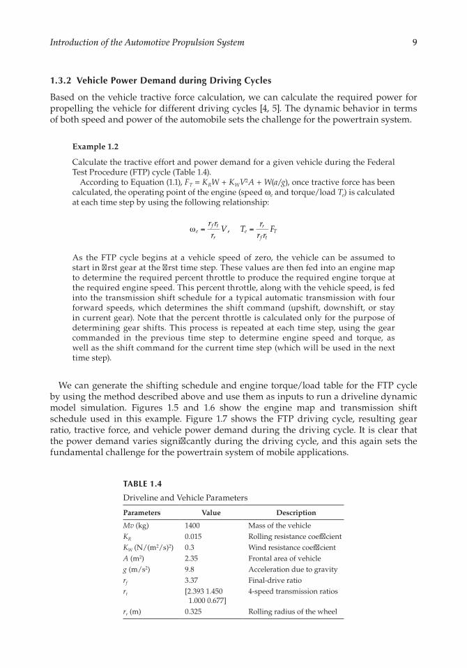
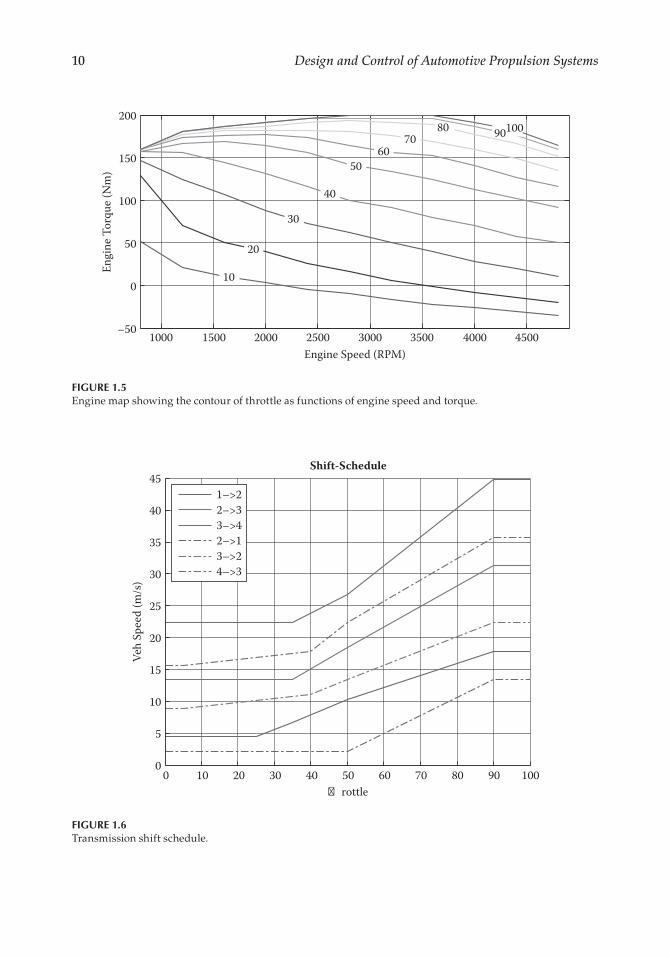
We can generate the shifting schedule and engine torque/load table for the FTP cycle by using the method described above and use them as inputs to run a driveline dynamic model simulation. Figures 1.5 and 1.6 show the engine map and transmission shift schedule used in this example. Figure 1.7 shows the FTP driving cycle, resulting gear ratio, tractive force, and vehicle power demand during the driving cycle. It is clear that the power demand varies significantly during the driving cycle, and this again sets the fundamental challenge for the powertrain system of mobile applications.
TABLE 1.4
Driveline and Vehicle Parameters
Parameters Value Description
Mv (kg) 1400 Mass of the vehicleKR 0.015 Rolling resistance coefficientKW (N/(m2/s)2) 0.3 Wind resistance coefficientA (m2) 2.35 Frontal area of vehicleg (m/s2) 9.8 Acceleration due to gravityrf 3.37 Final-drive ratio rt [2.393 1.450
1.000 0.677]4-speed transmission ratios
rr (m) 0.325 Rolling radius of the wheel
10 Design and Control of Automotive Propulsion Systems
2001009080
7060
50
40
30
20
10
1000 1500 2000 2500 3000Engine Speed (RPM)
Engi
ne T
orqu
e (N
m)
3500 4000 4500–50
0
50
100
150
FIGURE 1.5Engine map showing the contour of throttle as functions of engine speed and torque.
1009080706050�rottle
Shift-Schedule
Veh
Spee
d (m
/s)
1–>245
0
5
10
15
20
25
35
30
40 2–>33–>42–>13–>24–>3
403020100
FIGURE 1.6Transmission shift schedule.

11Introduction of the Automotive Propulsion System
References
1. E. Burke, L.H. Nagler, E.C. Campbell, L.C. Lundstron, W.E. Zierer, H.L. Welch, T.D. Kosier, and W.A. McConnell, Where Does All the Power Go? SAE Technical Paper 570058, 1957.
2. P.N. Blumberg, Powertrain Simulation: A Tool for the Design and Evaluation of Engine Control Strategies in Vehicles, SAE Technical Paper 760158, 1976.
3. R.A. Bechtold, Ingredients of Fuel Economy, SAE Technical Paper 790928, 1979.
0 200 400 600 800 1000 1200 1400 1600 18000
10
20
30
Time (s)
Vehi
cle S
peed
(m/s
)FTP Cycle
0 200 400 600 800 1000 1200 1400 1600 18001
2
3
4
Time (s)
Tran
smiss
ion
Gea
r
0 200 400 600 800 1000 1200 1400 1600 1800–2000
0
2000
Time (s)
Trac
tive E
�ort
(N)
0 200 400 600 800 1000 1200 1400 1600 1800
–20
0
20
40
Time (s)
Pow
er (k
W)
FIGURE 1.7The FTP driving cycle, the gear ratio, the tractive effort, and the vehicle power demand.

12 Design and Control of Automotive Propulsion Systems
4. V. Mallela, Design, Modeling and Control of a Novel Architecture for Automatic Transmission Systems, Master of Science thesis, University of Minnesota, Twin Cities, May 2013.
5. A. Heinzen, P. Gillella, and Z. Sun, Iterative Learning Control of a Fully Flexible Valve Actuation System for Non-Throttled Engine Load Control, Control Engineering Practice, 19(12): 1490–1505, 2011.
13
2Design, Modeling, and Control of Internal Combustion Engine
2.1 Introduction to Engine Subsystems
The engine subsystems can be divided into the fuel system, ignition system, valve system, exhaust gas recirculation system, turbo-compressor system, etc. This chapter mainly dis-cusses the design, modeling, and control of these subsystems.
For control strategy development, zero-dimensional mean value engine models are widely used [1, 2], due to their simplicity and low simulation throughput. For the engine air handling system or crankshaft dynamics, mean value models are accurate enough since the piston reciprocating movement has less impact on these subsystems than on the combustion process. Therefore, the mean value modeling approach is often used for these subsystems. The disadvantage of mean value engine modeling is that it does not provide detailed information about the engine combustion process, such as in-cylinder gas pres-sure, temperature, and ionization signals, which have been widely used for closed-loop combustion control [3–5]. The in-cylinder pressure rise is also a key indicator for detecting engine knock [6].
In order to explore the details about the engine combustion process, multizone, three- dimensional computational fluid dynamics (CFD) models with detailed chemical kinet-ics are presented in [7–9] that describe the thermodynamic, fluid flow, heat transfer, and pollutant formation phenomena of the homogeneous charge compression ignition (HCCI) combustion. Similar combustion models have also been implemented into commercial codes such as GT-Power [10] and Wave. However, these high-fidelity models cannot be directly used for control strategy development since they are too complicated to be used for real-time simulations, but they can be used as reference models for developing simplified (or control-oriented) combustion models for control development and validation purposes.
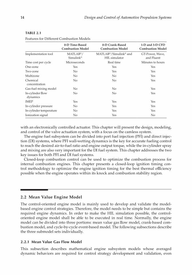
For real-time hardware-in-the-loop (HIL) simulations, it is necessary to develop a type of combustion model with its complexity in between the time-based mean value models and the CFD models. This motivates the combustion modeling work presented in this chapter. The zero-dimensional (0-D) crank-based combustion model is described in this chapter. Table 2.1 compares the capability of this modeling method with the other two.
The engine valve actuation subsystem employs a camshaft to open and close poppet-type intake and exhaust valves. The camshaft is connected to the crankshaft mechanically to ensure synchronized motion between the intake and exhaust valves and the piston motion. To improve the flexibility of the valve actuation system, a variable valve timing system, variable valve lift, and duration system have been designed to enhance the existing camshaft-based system. Camless systems have also been proposed to replace the camshaft
14 Design and Control of Automotive Propulsion Systems
with an electronically controlled actuator. This chapter will present the design, modeling, and control of the valve actuation system, with a focus on the camless system.
The engine fuel subsystem can be divided into port fuel injection (PFI) and direct injec-tion (DI) systems, where PFI wall-wetting dynamics is the key for accurate fueling control to reach the desired air-to-fuel ratio and engine output torque, while the in-cylinder spray and mixing are also very important for the DI fuel system. This chapter addresses the two key issues for both PFI and DI fuel systems.
Closed-loop combustion control can be used to optimize the combustion process for internal combustion engines. This chapter presents a closed-loop ignition timing con-trol methodology to optimize the engine ignition timing for the best thermal efficiency possible when the engine operates within its knock and combustion stability region.
2.2 Mean Value Engine Model
The control-oriented engine model is mainly used to develop and validate the model-based engine control strategies. Therefore, the model needs to be simple but contains the required engine dynamics. In order to make the HIL simulation possible, the control-oriented engine model shall be able to be executed in real time. Normally, the engine model can be divided into three portions: mean value gas flow model, crank-based com-bustion model, and cycle-by-cycle event-based model. The following subsections describe the three submodel sets individually.
2.2.1 Mean Value Gas Flow Model
This subsection describes mathematical engine subsystem models whose averaged dynamic behaviors are required for control strategy development and validation, even
TABLE 2.1
Features for Different Combustion Models
0-D Time-Based Combustion Model
0-D Crank-Based Combustion Model
1-D and 3-D CFD Combustion Model
Implementation tool MATLAB®/Simulink®
MATLAB®/Simulink® and HIL simulator
GT-Power, Wave, and Fluent
Time cost per cycle Microseconds Real time Minutes to hoursOne-zone Yes Yes YesTwo-zone No Yes YesMultizone No No YesChemical concentration
No No Yes
Gas-fuel mixing model No No YesIn-cylinder flow dynamics
No No Yes
IMEP Yes Yes YesIn-cylinder pressure No Yes YesIn-cylinder temperature No Yes YesIonization signal No Yes No
15Design, Modeling, and Control of Internal Combustion Engine
though they are functions of the engine reciprocating phenomenon. All parameters and variables used in these models are functions of time t.
2.2.1.1 Valve Dynamic Model
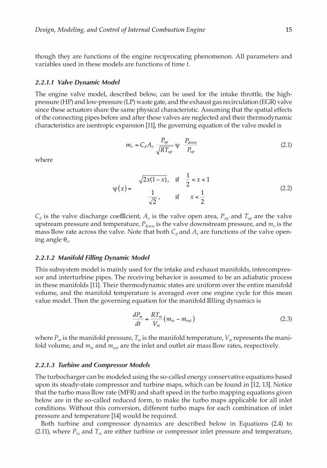
The engine valve model, described below, can be used for the intake throttle, the high- pressure (HP) and low-pressure (LP) waste gate, and the exhaust gas recirculation (EGR) valve since these actuators share the same physical characteristic. Assuming that the spatial effects of the connecting pipes before and after these valves are neglected and their thermodynamic characteristics are isentropic expansion [11], the governing equation of the valve model is
m C APRT
PP
v d vup
up
down
up= ψ (2.1)
where
xx x x
x
2 (1 ), if12
1
12
, if12
( )ψ =− < <
< (2.2)
Cd is the valve discharge coefficient, Av is the valve open area, Pup and Tup are the valve upstream pressure and temperature, Pdown is the valve downstream pressure, and mv is the mass flow rate across the valve. Note that both Cd and Av are functions of the valve open-ing angle θv.
2.2.1.2 Manifold Filling Dynamic Model
This subsystem model is mainly used for the intake and exhaust manifolds, intercompres-sor and interturbine pipes. The receiving behavior is assumed to be an adiabatic process in these manifolds [11]. Their thermodynamic states are uniform over the entire manifold volume, and the manifold temperature is averaged over one engine cycle for this mean value model. Then the governing equation for the manifold filling dynamics is
dPdt
RTV
m mm m
min out( )= − (2.3)
where Pm is the manifold pressure, Tm is the manifold temperature, Vm represents the mani-fold volume, and min and mout are the inlet and outlet air mass flow rates, respectively.
2.2.1.3 Turbine and Compressor Models
The turbocharger can be modeled using the so-called energy conservative equations based upon its steady-state compressor and turbine maps, which can be found in [12, 13]. Notice that the turbo mass flow rate (MFR) and shaft speed in the turbo mapping equations given below are in the so-called reduced form, to make the turbo maps applicable for all inlet conditions. Without this conversion, different turbo maps for each combination of inlet pressure and temperature [14] would be required.
Both turbine and compressor dynamics are described below in Equations (2.4) to (2.11), where Pin and Tin are either turbine or compressor inlet pressure and temperature,

16 Design and Control of Automotive Propulsion Systems
Pout and Tout are either turbine or compressor outlet pressure and temperature, Nturbo is the turbocharger shaft speed in rpm, and η denotes thermal efficiency.
1. Turbine mapping: Turbine maps, fturb and f′turb, in Equations (2.4) and (2.5) are used to calculate the reduced MFR mturb and thermal efficiency ηturb based on pressure ratio across the turbine and the reduced turbo shaft speed. The actual MFR can be calculated from the reduced MFR mturb by
,m fPP
NT
PT
turb turbin
out
turbo
in
in
in
= (2.4)
and
,fPP
NT
turb turbin
out
turbo
in
η = (2.5)
2. Compressor mapping: Compressor maps, fcomp and f′comp, in Equations (2.6) and (2.7) are used to calculate the compressor pressure ratio and thermal efficiency ηcomp based on reduced MFR mcomp and reduced turbo shaft speed by
,PP
fm T
PN
Tout
incomp
comp in
in
turbo
in
= (2.6)
and
,fm T
PN
Tcomp comp
comp in
in
turbo
in
η = (2.7)
3. Temperature calculation: The outlet temperature of the turbine or compressor can be calculated based upon:
TT
PP
out
in
out
in=
( )κ−
κ
1
(2.8)
Notice that Equation (2.8) assumes isentropic gas expansion and the compressing process for either turbine or compressor. However, the actual physical process is not isentropic, leading to more enthalpy remaining in the gas due to thermal efficiency, which makes the actual outlet temperature higher than that given by Equation (2.8), but the difference is relatively small. Simulation results presented in [15] show an acceptable correlation between GT-Power simulation results and the tempera-ture calculated using Equation (2.8). Therefore, this assumption is acceptable.
4. Turbine power calculation: The power generated by the turbine, denoted as Eturb, is calculated by
1
1
E m C TPP
turb turb p turb inout
in= η −
κ−κ
(2.9)
17Design, Modeling, and Control of Internal Combustion Engine
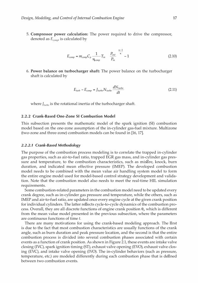
5. Compressor power calculation: The power required to drive the compressor, denoted as Ecomp, is calculated by
1
1
1
E m C TPP
comp comp pcomp
inout
in=
η−
κ−κ
(2.10)
6. Power balance on turbocharger shaft: The power balance on the turbocharger shaft is calculated by
E E J NdN
dtturb comp turbo turbo
turbo− = (2.11)
where Jturbo is the rotational inertia of the turbocharger shaft.
2.2.2 Crank-Based One-Zone SI Combustion Model
This subsection presents the mathematic model of the spark ignition (SI) combustion model based on the one-zone assumption of the in-cylinder gas-fuel mixture. Multizone (two-zone and three-zone) combustion models can be found in [16, 17].
2.2.2.1 Crank-Based Methodology
The purpose of the combustion process modeling is to correlate the trapped in-cylinder gas properties, such as air-to-fuel ratio, trapped EGR gas mass, and in-cylinder gas pres-sure and temperature, to the combustion characteristics, such as misfire, knock, burn duration, and indicated mean effective pressure (IMEP). The developed combustion model needs to be combined with the mean value air handling system model to form the entire engine model used for model-based control strategy development and valida-tion. Note that the combustion model also needs to meet the real-time HIL simulation requirements.
Some combustion-related parameters in the combustion model need to be updated every crank degree, such as in-cylinder gas pressure and temperature, while the others, such as IMEP and air-to-fuel ratio, are updated once every engine cycle at the given crank position for individual cylinders. The latter reflects cycle-to-cycle dynamics of the combustion pro-cess. Overall, they are all discrete functions of engine crank position θi, which is different from the mean value model presented in the previous subsection, where the parameters are continuous functions of time t.
There are many motivations for using the crank-based modeling approach. The first is due to the fact that most combustion characteristics are usually functions of the crank angle, such as burn duration and peak pressure location, and the second is that the entire combustion process is divided into several combustion phases associated with certain events as a function of crank position. As shown in Figure 2.1, these events are intake valve closing (IVC), spark ignition timing (ST), exhaust valve opening (EVO), exhaust valve clos-ing (EVC), and intake valve opening (IVO). The in-cylinder behaviors (such as pressure, temperature, etc.) are modeled differently during each combustion phase that is defined between two combustion events.
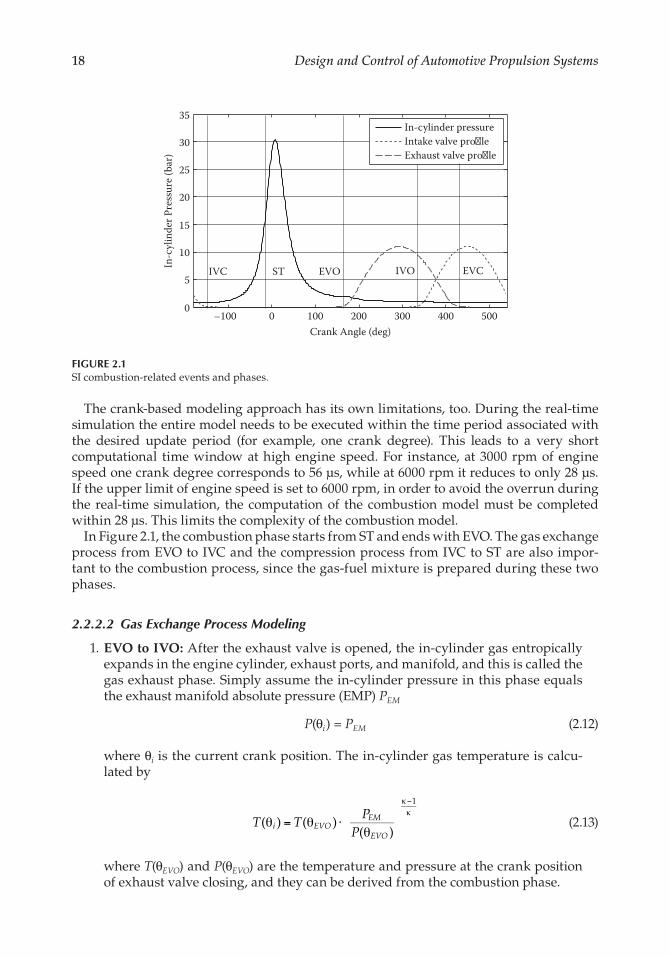
18 Design and Control of Automotive Propulsion Systems
The crank-based modeling approach has its own limitations, too. During the real-time simulation the entire model needs to be executed within the time period associated with the desired update period (for example, one crank degree). This leads to a very short computational time window at high engine speed. For instance, at 3000 rpm of engine speed one crank degree corresponds to 56 μs, while at 6000 rpm it reduces to only 28 μs. If the upper limit of engine speed is set to 6000 rpm, in order to avoid the overrun during the real-time simulation, the computation of the combustion model must be completed within 28 μs. This limits the complexity of the combustion model.
In Figure 2.1, the combustion phase starts from ST and ends with EVO. The gas exchange process from EVO to IVC and the compression process from IVC to ST are also impor-tant to the combustion process, since the gas-fuel mixture is prepared during these two phases.
2.2.2.2 Gas Exchange Process Modeling
1. EVO to IVO: After the exhaust valve is opened, the in-cylinder gas entropically expands in the engine cylinder, exhaust ports, and manifold, and this is called the gas exhaust phase. Simply assume the in-cylinder pressure in this phase equals the exhaust manifold absolute pressure (EMP) PEM
P(θi ) = PEM (2.12)
where θi is the current crank position. The in-cylinder gas temperature is calcu-lated by
( ) ( )( )
1
T TP
Pi EVO
EM
EVOθ = θ ⋅
θ
κ−κ
(2.13)
where T(θEVO) and P(θEVO) are the temperature and pressure at the crank position of exhaust valve closing, and they can be derived from the combustion phase.
–100 0 100 200 300 400 5000
5
10
15
20
25
30
35
Crank Angle (deg)
In-c
ylin
der P
ress
ure (
bar)
In-cylinder pressureIntake valve pro�leExhaust valve pro�le
IVC ST EVO IVO EVC
FIGURE 2.1SI combustion-related events and phases.

19Design, Modeling, and Control of Internal Combustion Engine
2. IVO to EVC: This phase is usually called valve overlap phase. During this phase the intake valve starts to open while the exhaust valve is closing. The opening of both valves makes the flow dynamics more complicated and difficult to model. For simplicity, assume the in-cylinder gas pressure equals the mean value of the pressures in exhaust manifold and intake manifold. That is,
( )2
PP P
iEM IMθ =
+ (2.14)
where PIM is the intake manifold absolute pressure. The gas temperature can be calculated the same as in the last phase:
( ) ( )2 ( )
1
T TP P
Pi IVO
EM IM
IVOθ = θ
+θ
κ−κ
(2.15)
In addition, at EVC the residual gas mass is calculated based on ideal gas law as follows:
( ) ( )
( )M
P VT R
rEVC EVC
EVC=
θ θθ
(2.16)
3. EVC to IVC: During this phase fresh air is trapped inside the engine cylinder. The in-cylinder pressure is mainly influenced by intake manifold pressure, but not always equal to it. It can be calculated by
P(θi) = PIMηIN (2.17)
where ηIN is actually the volumetric efficiency of the intake process, and it is a function of engine speed Ne and engine load PIM. In-cylinder gas temperature is calculated by
( ) ( )( )
1
T TPP
i EVCIM IN
EVCθ = θ
ηθ
κ−κ
(2.18)
Additionally, the total mass of in-cylinder gas mixture for the compression and combustion phases is calculated at IVC, also based on the ideal gas law, as follows:
( ) ( )
( )( )
( )M
P VT R
P VT R
tIVC IVC
IVCIN
IM IVC
IVC=
θ θθ
= ηθ
θ (2.19)
4. IVC to ST: This phase is the compression phase without combustion. The governing equations of this phase are also based on the isentropic law of ideal gas. They are
( ) ( )( )( )1
1P PVV
i ii
iθ = θ
θθ
−−
κ
(2.20)

20 Design and Control of Automotive Propulsion Systems
and
( ) ( )( )( )1
11
T TVV
i ii
iθ = θ
θθ
( )
−−
κ−
(2.21)
where V(θi) is the cylinder volume at crank position V(θi) and is calculated by
( )12
11
cos( )2
sin ( )4
2
22
2
Vr
LS
LS
B Si
iiθ = +
−+ −
θ− − θ
π (2.22)
Note that r is compression ratio, L is connecting rod length, S is piston stroke, and B is piston bore. The values of the sample parameters can be found in [15].
2.2.2.3 One-Zone SI Combustion Model
In the SI combustion model, the start of combustion is initiated by the spark ignition, which can be controlled at any desired crank position defined as spark timing (ST). After ST the mass fraction burned of trapped fuel can be represented by an S-shaped Wiebe function [19] as
( ) 1 exp1
x aii ST
SI
m
θ = − −θ − θ
θ
+
(2.23)
where ΔθSI is the predicted burn duration of the SI combustion mode (a calibration param-eter of engine speed, engine load, often represented by the manifold air pressure (MAP), and coolant temperature), and m is the Wiebe exponent (m = 2 was used in the model). Coefficient a depends on how the burn duration ΔθSI is defined. In case ΔθSI is defined as the duration of the 10% to 90% MFB, a can be calculated by
ln(1 0.9)1
1 ln(1 0.1)1
1
1
a m m
m
[ ] [ ]= − − + − − − +
+
(2.24)
Assuming both burned and unburned gases are evenly mixed in one zone, the SI com-bustion process is simplified into a heat transfer with a volume change process of the entire in-cylinder gas. The in-cylinder gas temperature can be calculated by
T TVV
M H x x QM C
i ii
i
SI f LHV i i i
t v( ) ( )
( )( )
( ) ( ) ( )1
11
1[ ]θ = θ
θθ
+η θ − θ − θ
( )
−−
κ−− (2.25)
where ηSI is the function of engine speed and load, calibrated by matching the calcu-lated IMEP with that given by GT-Power, and Q represents the heat transfer between the in- cylinder gas and cylinder inner surface. Only convection was considered in the
21Design, Modeling, and Control of Internal Combustion Engine
model, since for a gasoline engine the heat transfer due to radiation is relatively small in comparison with the convective heat transfer [20]. The Woschni correlation model [21, 22] is used to calculate the heat transfer term:
Q(θi) = Ac hc [T(θi−1) − Tw] (2.26)
where hc is called the Woschni correlation, and it can be written as
1 0.75 1.62
hcB P w T
Nc
m m m m
e=
− −
(2.27)
The coefficients c and exponent m in Equation (2.27) can be used to correlate the simulation results to the experimental data or GT-Power simulation results; c = 0.54 and m = 0.8 were found to have good correlation for the model in the result presented in Chapter 5.
There are two terms on the right-hand side of Equation (2.25). The first term represents an isentropic compressing or expanding process, while the second term calculates the temperature rise due to the heat transfer during the combustion. Therefore, the compli-cated thermodynamic process of the combustion is simplified into an isentropic volume change process without heat exchange in one crank degree period and the heat absorption from combusted fuel without volume change in an infinitely small time period. Based on the updated gas temperature from Equation (2.25), the gas pressure can be calculated by applying ideal gas law to the in-cylinder gas as follows:
( ) ( )( )( )
( )( )1
1
1P P
VV
TT
i ii
i
i
iθ = θ ⋅
θθ
⋅θθ
−−
−
(2.28)
2.2.3 Combustion Event-Based Dynamic Model
Due to the cycle-by-cycle combustion event, certain engine dynamics need to be modeled event by event such as fuel injection process and exhaust gas recirculation (EGR).
2.2.3.1 Fueling Dynamics and Air-to-Fuel Ratio Calculation
The engine system could be equipped with port fuel injection (PFI), direct injection (DI), or both PFI and DI systems. Since the fuel injected by the DI fuel system is trapped in the cylinder directly and will not affect the fueling quantity for the next cycle, the DI fuel injection dynamics is normally ignored. For the PFI fuel injection system, the wall-wetting phenomenon of the PFI fuel spray on the intake port and the back of the intake valve intro-duces cycle-to-cycle dynamics and affects the engine transient performance significantly, and it needs to be modeled in the engine model.
The wall-wetting phenomenon of the PFI fuel injection can be described in such a way that only part of the injected fuel (β · Minj, 0 < β < 1) enters the cylinder while the rest of the fuel ((1 – β) · Minj) remains on the surface of the intake port and the back of intake valves. Then the total fuel mass flow into the cylinder consists of the fuel directly injected into the cylinder and the fuel vapor (α · Mres, 0 < α < 1) from fuel mass stored on the intake port and the back of the intake valves from previous injection. The wall-wetting phenomenon leads to the most important dynamics in PFI fuel mass calculation, which affects engine
22 Design and Control of Automotive Propulsion Systems
transient performance significantly [18]. The governing equation of the wall-wetting dynamics can be expressed as
1
1 1 1
M k M k M k
M k M k M k
fuel res inj
res res inj
[ ] [ ] [ ][ ] [ ] [ ]( )( )
= α ⋅ − + β ⋅
= − α ⋅ − + − β ⋅ (2.29)
where k is an index representing the engine cycle number (k indicates current engine cycle and k – 1 the last engine cycle), Mfuel is the quantity of fuel mass flowed into the cylinder, Mres is the quantity of fuel mass left on the port and the back of intake valves, Minj is the amount of fuel injected by the PFI injector at the given engine cycle, and coefficients α and β are functions of engine coolant temperature, engine speed, and load.
The engine gas exchange behavior introduces dynamics to the air-to-fuel ratio calcula-tion too, since a substantial portion of the burned gas remains inside the cylinder, espe-cially at low load. This gas fraction carries the air-to-fuel ratio of the previous engine cycle to the current one. Therefore, the air-to-fuel ratio can be modeled cycle-by-cycle below:
[ ][ ] [ ] [ 1] [ 1] [ 1]
[ ]k
k M k M k k M kM k
f t r r
t
( )λ =
λ − − + λ − ⋅ − (2.30)
where λ is the normalized air-to-fuel ratio of the gas mixture inside the engine cylinder after IVC, λf is the normalized air-to-fuel ratio of the fresh charge in the current cycle and it is defined as
[ ][ ] [ 1]
[ ](1 )k
M k M kM k
ft r
fuelλ =
− −+ σ
(2.31)
and σ is stoichiometric air-to-fuel ratio of the fuel.
2.2.3.2 Engine Torque and Crankshaft Dynamic Model
The equations presented in the last subsections provide a complete cycle profile of in-cylinder gas pressure. Based on this pressure profile and the cylinder volume profile, the engine IMEP can be calculated by a simple digital integration:
1
1
0
719
PV
P V VIMEPd
i i i
i
i
∑{ }( ) ( ) ( )= ⋅ θ ⋅ θ − θ −
=
=
(2.32)
where Vd is the cylinder displacement and
Vd = V (θBDC) − V (θTDC) (2.33)
At last engine torque output is calculated by
60 ( )
2T
n P P VN
eIMEP FMEP d
e=
−π
(2.34)
where PFMEP is the friction mean effective pressure and n is the quantity of engine cylinders.
23Design, Modeling, and Control of Internal Combustion Engine
Based upon Newton theory, assuming a rigid crankshaft, it can be derived as
602
dNdt
T TJ
e e l
e=
π−
(2.35)
where Je is the rotational inertia of the engine crankshaft; Te and Tl are the engine brake and load torques, respectively. Note that simulations Tl can be generated by an engine dynamometer model controlled by a proportional-integral-derivative (PID) feedback con-troller to maintain the desired engine speed.
2.3 Valve Actuation System
2.3.1 Valve Actuator Design
Poppet-type intake and exhaust valves are widely used to control the fresh charge and exhaust gas exchange dynamics during the intake and exhaust strokes of the internal combustion engine (ICE). The valves are actuated with one or two camshafts that are con-nected to the crankshaft mechanically. There are mainly three different arrangements for the valve actuation system. The direct acting system has the cam lobe in contact with the follower and the engine valve in a vertical arrangement. The roller finger follower system uses a lever to actuate the valve, and the cam lobe is in contact with a roller that is mounted on the lever between the valve and the pivoting point. The pushrod system installs the camshaft in the valley of the engine and uses a pushrod to actuate the valve through a lever. The roller finger follower system has the smallest effective mass, while the pushrod system is heavier than the other two systems due to the long connecting rod. The roller finger follower system also has less friction due to the rolling contact. The direct acting system has the largest friction for its sliding friction. The pushrod system is more suitable for low- to medium-speed operation, and the direct acting system is capable of high-speed engine operation. From the packaging perspective, the pushrod system is able to reduce the overall height of the engine since the camshaft is housed in the valley of the engine.
A conventional valvetrain with fixed valve motion prevents real-time optimization of the air management system. Flexible intake or exhaust valve motions can greatly improve the fuel economy, emissions, and torque output performance of the internal combustion engine. Flexible valve actuation can be achieved with mechanical (cam-based), electromag-netic (electromechanical), electrohydraulic, and electropneumatic valvetrain mechanisms. The cam-based mechanisms offer limited flexibility of the valve event and are designed as multiple-step devices or continuously variable devices. The multistep cam mecha-nism [23], for example, allows switching between two (or three) discrete cams. The cam phasing mechanism [24, 25] allows the intake or exhaust cams to be continuously phase shifted, however, without the flexibility of changing the valve lift or duration. The vari-able valve lift system [26] has incorporated a combination of variable cam phasing with a continuously variable valve lift mechanism, which provides significant flexibility, but at relatively high cost and complexity. A fully flexible valve actuation system, often referred to as camless valvetrain, includes electromagnetic (electromechanical), electrohydraulic, and electropneumatic systems. The electromagnetic systems [27] are able to generate flex-ible valve timing and duration. These devices, however, generally have high valve seating velocity and are limited by the inherent fixed valve lift operation. The electrohydraulic

24 Design and Control of Automotive Propulsion Systems
systems [28–32] also provide fully flexible control of the valve lift events. For these systems, digital or proportional valves are used to control the hydraulic fluid to actuate the engine valve. The potential issues with the electrohydraulic systems are energy consumption and reliability of generating a repeatable valve profile over the life cycle of the engine. Electropneumatic systems [33, 34] employ pneumatic actuators to drive the engine valve. Potential issues with the electropneumatic systems include low power density and com-pressibility of air. Due to the above challenges, currently there is no mass-produced fully flexible valve actuation system on the market.
Motivations for developing fully flexible valve actuation (FFVA) systems come from three areas. First, the FFVA system offers significant fuel economy benefits, lower emissions, and better torque output performance. Second, the FFVA systems could enable various engine operating strategies such as nonthrottling load control, cylinder deactivation, internal exhaust gas recirculation (EGR) control, homogeneous charge compression ignition, switch-ing or combining engine operation modes, etc. Third, the FFVA system could also provide a common platform that delivers the functions of throttle, EGR, cam phaser, cylinder deacti-vation, port deactivation, two-step cam, and continuously variable lift systems. This would reduce the development time and cost compared with separately developed systems.
Besides the above production-oriented systems, laboratory FFVA systems have also been developed [35–39]. These laboratory FFVA systems have been used to explore vari-ous advanced combustion concepts, and the results have shown significant fuel economy, emissions, and performance improvement. More importantly, from the valve actuation perspective, they demonstrate the feasibility of operating FFVA systems safely and reliably in the laboratory environment.
2.3.1.1 Challenges for Developing FFVA Systems
A production-viable FFVA system must be able to generate precise and robust valve motion with high efficiency and simplified control. In this section we will outline the tech-nical challenges for developing FFVA systems and their implications to system design and control. While the challenges are common to any type of FFVA systems, including electro-magnetic, electrohydraulic, and electropneumatic systems, we will focus on the electrohy-draulic system in this section.
2.3.1.1.1 Precise and Robust Motion
For fully flexible valve actuation systems, without proper planning and control, it is pos-sible to have mechanical interference between the piston and valves or between the engine valves. So precise valve motion is required to prevent mechanical interference. As the valve lift profile controls the airflow and residual level inside the combustion chamber, it becomes necessary to have accurate and consistent valve lift profiles to achieve high- performance engine operation. This consistency requirement includes both cycle-to-cycle and cylinder-to-cylinder repeatability of the valve lift profiles. The impact speed dur-ing the valve closing event is called seating velocity. Acceptable valve seating velocity is required to minimize valvetrain noise and maximize valve and valve seat durability.
2.3.1.1.2 Energy Efficiency
The FFVA system must be energy-efficient so that it can not only improve combustion efficiency, but also reduce the amount of energy required to actuate the valvetrain system. For electrohydraulic systems, pump efficiency, throttling of the high-pressure fluid, and parasitic losses due to leakage, etc., are the major sources of energy loss. For conventional
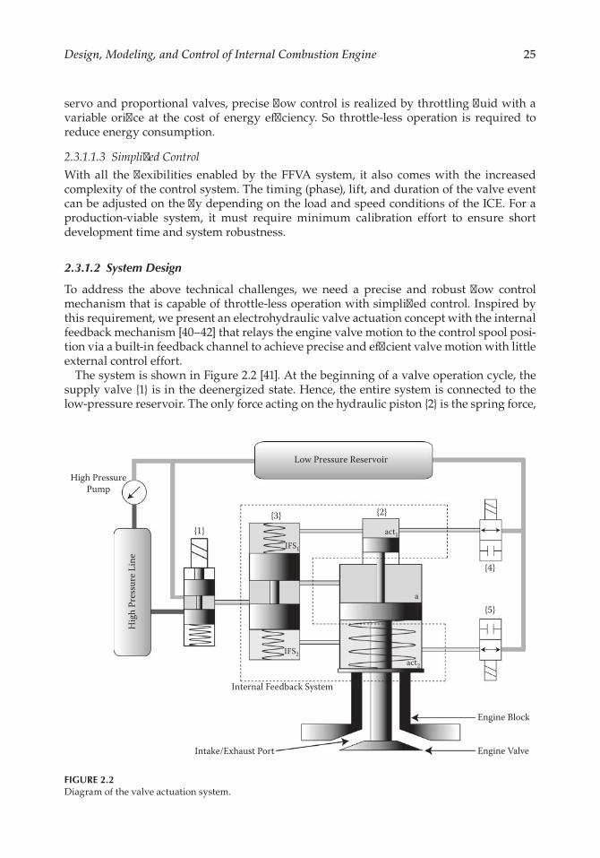
25Design, Modeling, and Control of Internal Combustion Engine
servo and proportional valves, precise flow control is realized by throttling fluid with a variable orifice at the cost of energy efficiency. So throttle-less operation is required to reduce energy consumption.
2.3.1.1.3 Simplified Control
With all the flexibilities enabled by the FFVA system, it also comes with the increased complexity of the control system. The timing (phase), lift, and duration of the valve event can be adjusted on the fly depending on the load and speed conditions of the ICE. For a production-viable system, it must require minimum calibration effort to ensure short development time and system robustness.
2.3.1.2 System Design
To address the above technical challenges, we need a precise and robust flow control mechanism that is capable of throttle-less operation with simplified control. Inspired by this requirement, we present an electrohydraulic valve actuation concept with the internal feedback mechanism [40–42] that relays the engine valve motion to the control spool posi-tion via a built-in feedback channel to achieve precise and efficient valve motion with little external control effort.
The system is shown in Figure 2.2 [41]. At the beginning of a valve operation cycle, the supply valve {1} is in the deenergized state. Hence, the entire system is connected to the low-pressure reservoir. The only force acting on the hydraulic piston {2} is the spring force,
High PressurePump
{1}{3} {2}
{4}
{5}
IFS1
IFS2
act1
act2
a
Engine Block
Low Pressure Reservoir
Hig
h Pr
essu
re L
ine
Engine ValveIntake/Exhaust Port
Internal Feedback System
FIGURE 2.2Diagram of the valve actuation system.
26 Design and Control of Automotive Propulsion Systems
which holds the engine valve in the closed position. Both on-off valves {4 and 5} are open, and hence all the feedback chambers are at the low pressure, and the spool of the feedback regulator {3} is balanced in the center position. To open the engine valve, the system is connected to the high-pressure line by energizing the supply valve. When the pressure in the actuation chamber overcomes the spring force, it accelerates the hydraulic piston downward. When the engine valve reaches a desired lift, the bottom on-off valve {5} is shut off, which restricts the fluid flow from the bottom feedback chamber to the reservoir and diverts it into the bottom chamber of the feedback regulator, and thus deflects the spool upward. As the spool moves upward, the orifice area of the spool valve decreases and thus restricts the fluid flow through it. This reduces the pressure in the actuation chamber and causes the hydraulic piston to decelerate. The synchronized motion between the hydraulic piston and the spool valve will continue until flow to the actuation chamber is completely shut off by the spool and the piston comes to a stop smoothly. Hence, by controlling the timing of the bottom on-off valve, we can control the maximum lift of the engine valve. To close the engine valve, the supply valve is first deenergized. The bottom on-off valve is then opened, which causes the spool of the regulator to return to the center position, and thus connects the actuation chamber to the low-pressure reservoir. The spring force becomes dominant, and hence moves the hydraulic piston upward, which starts to close the engine valve. The top on-off valve {4} is closed when the engine valve is near the seat. By the same principle, as explained previously, the spool is deflected in the downward direction, which decreases the orifice area and thus restricts the flow out of the actuation chamber. The actuation chamber pressure thus increases, which gradually decelerates the engine valve until it lands on the valve seat with a desired seating velocity. Hence, by just controlling the timing of the three valves (the solenoid valve and the on-off valves), the valve timing, lift, duration, and seating velocity can all be controlled precisely. In addi-tion to the effective valve motion control, this system has another advantage. The internal feedback mechanism is a very stiff hydromechanical system and has a very fast response when compared with electromechanical feedback loops. It can be engaged at the last moment possible and would thus lead to throttle-free operation during a major portion of the engine valve cycle. This leads to a minimization of throttling losses, and hence results in a decrease in power consumption.
Detailed dynamics models of the system have been built. The comparison between the model prediction and experimental results is shown in Figure 2.3 [41]. The results clearly demonstrate the precise control of valve lift, seating velocity, and duration.
2.3.2 Valve Actuator Model and Control
For fully flexible valve actuation systems, since there is no mechanical link between the crankshaft and the engine valve, feedback control is critical to achieve precise valve motion. Control system design for FFVA systems has been explored by a number of researchers. Richman and Reynolds [35] presented the development of an electro-hydraulic valve actuation system. An analog controller was used to regulate the valve motion. Performance degradation was observed at high engine speed due to limited bandwidth of the controller. Anderson et al. [43] presented an adaptive peak lift control for an electrohydraulic system. Valve event consistency was affected by the nonlinearity of the device and slow response of the solenoid valve. Misovec et al. [44] presented the digital valve technology applied to the control of a hydraulic valve actuator. Optimal control and proportional control were applied to drive the hydraulic valve to track a 1 Hz sinusoidal curve. Hoffmann and Stefanopoulou [45] reported simulation results

27Design, Modeling, and Control of Internal Combustion Engine
10Ex
p
Tim
e (s
)Ti
me
(s)
Tim
e (s
)
Tim
e (s
)Ti
me
(s)
Tim
e (s
)
Velocity (mm/s)
Velocity (mm/s)
Velocity (mm/s)
Lift (mm)
Lift (mm)
Lift (mm)
Sim
Exp
Sim
Exp
Sim
Exp
Sim
Exp
Sim
Exp
Sim
8 6 4 2 0 00.
020.
040.
06
10 8 6 4 2 0 00.
020.
040.
06
10 8 6 4 2 0 00.
020.
040.
06
3000
2000
1000
–100
00
–200
0
–300
0
3000
2000
1000
–100
00
–200
0
–300
0
3000
2000
1000
–100
00
–200
0
–300
00
0.02
0.04
0.06
00.
020.
040.
060
0.02
0.04
0.06
FIG
UR
E 2.
3C
ompa
riso
n be
twee
n m
odel
sim
ula
tion
and
exp
erim
enta
l res
ult
s.

28 Design and Control of Automotive Propulsion Systems
for the iterative learning control of an electromagnetic valve actuator to handle the gas flow force to improve system performance. Tai and Tsao [46] presented the modeling and control of an electromagnetic valve actuator. An LQ optimal control was used to achieve soft seating capability.
In this section we present the model and control for a FFVA system [47] to precisely track a desired valve profile that is generated electronically in real time based on the engine operating condition. Due to the four-stroke motion of the ICE, the valve profile is periodic to the rotational angle of the engine. With constant engine speed, the valve profile is also periodic in the time domain, and the lift, phase, and duration transients can be realized using robust repetitive control [48, 49]. When the engine speed varies, the period of the valve profile changes in real time. This phenomenon poses a fundamental challenge to the transient control problem and repetitive control cannot be applied anymore. To overcome this challenge, we use a new valve profile consisting of a periodic portion and a dwell portion with time-varying duration. Robust repetitive control is then applied to the peri-odic portion, and proportional plus integral and derivative control is applied to the dwell portion. These two controls are switched in real time to achieve asymptotic valve profile tracking performance. To demonstrate the effectiveness of the proposed control method, we show real-time valve lift profiles used to explore homogeneous charge compression ignition (HCCI) combustion at different engine operating conditions.
2.3.2.1 System Hardware and Dynamic Model
As shown in Figure 2.4 [47], the FFVA system includes a hydraulic pump, accumulators, servo valves, hydraulic pistons, linear variable differential transducers (LVDTs), encod-ers, signal conditioners, power amplifiers, and the control system. The hydraulic pump
Encoder Signal
ControlSystem Power
AmplierTorqueMotor
Engine Valve
Servo Valve
HydraulicPump
Accumulator
HydraulicPiston
LinearVariableDi�erentialTransducer
LVDT
FIGURE 2.4Block diagram of the FFVA system.
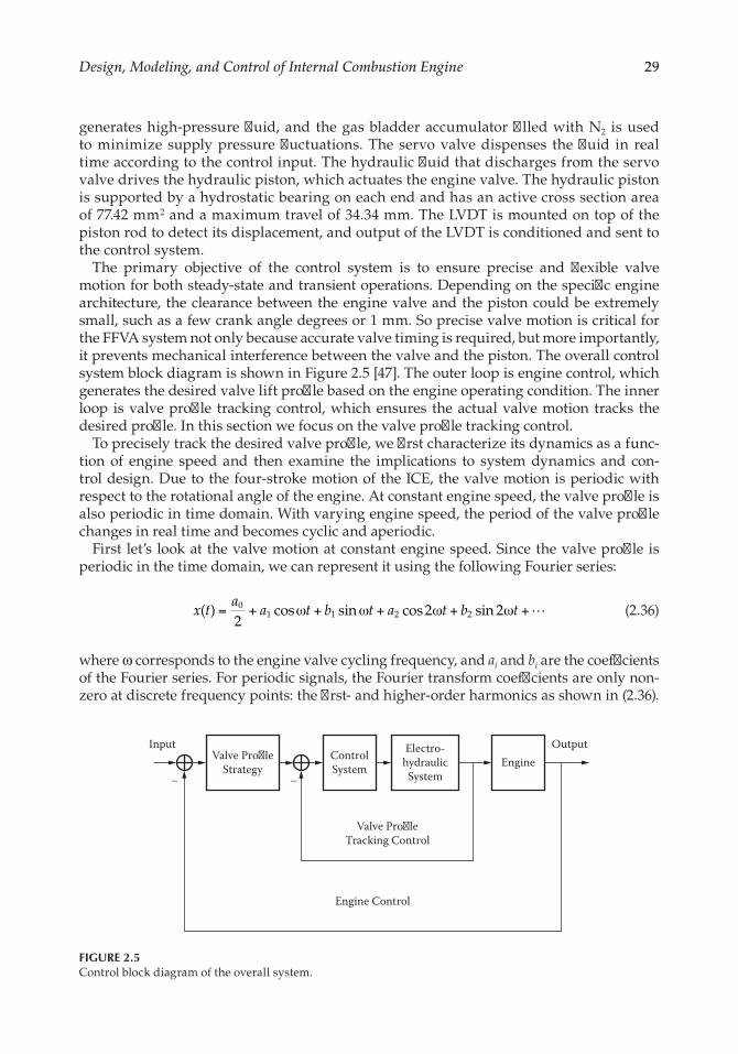
29Design, Modeling, and Control of Internal Combustion Engine
generates high-pressure fluid, and the gas bladder accumulator filled with N2 is used to minimize supply pressure fluctuations. The servo valve dispenses the fluid in real time according to the control input. The hydraulic fluid that discharges from the servo valve drives the hydraulic piston, which actuates the engine valve. The hydraulic piston is supported by a hydrostatic bearing on each end and has an active cross section area of 77.42 mm2 and a maximum travel of 34.34 mm. The LVDT is mounted on top of the piston rod to detect its displacement, and output of the LVDT is conditioned and sent to the control system.
The primary objective of the control system is to ensure precise and flexible valve motion for both steady-state and transient operations. Depending on the specific engine architecture, the clearance between the engine valve and the piston could be extremely small, such as a few crank angle degrees or 1 mm. So precise valve motion is critical for the FFVA system not only because accurate valve timing is required, but more importantly, it prevents mechanical interference between the valve and the piston. The overall control system block diagram is shown in Figure 2.5 [47]. The outer loop is engine control, which generates the desired valve lift profile based on the engine operating condition. The inner loop is valve profile tracking control, which ensures the actual valve motion tracks the desired profile. In this section we focus on the valve profile tracking control.
To precisely track the desired valve profile, we first characterize its dynamics as a func-tion of engine speed and then examine the implications to system dynamics and con-trol design. Due to the four-stroke motion of the ICE, the valve motion is periodic with respect to the rotational angle of the engine. At constant engine speed, the valve profile is also periodic in time domain. With varying engine speed, the period of the valve profile changes in real time and becomes cyclic and aperiodic.
First let’s look at the valve motion at constant engine speed. Since the valve profile is periodic in the time domain, we can represent it using the following Fourier series:
�x ta
a t b t a t b t( )2
cos sin cos2 sin 201 1 2 2= + ω + ω + ω + ω + (2.36)
where ω corresponds to the engine valve cycling frequency, and ai and bi are the coefficients of the Fourier series. For periodic signals, the Fourier transform coefficients are only non-zero at discrete frequency points: the first- and higher-order harmonics as shown in (2.36).
Engine Control
Valve Pro�leTracking Control
OutputInput
– –
Valve Pro�leStrategy
ControlSystem
Electro-hydraulicSystem
Engine
FIGURE 2.5Control block diagram of the overall system.
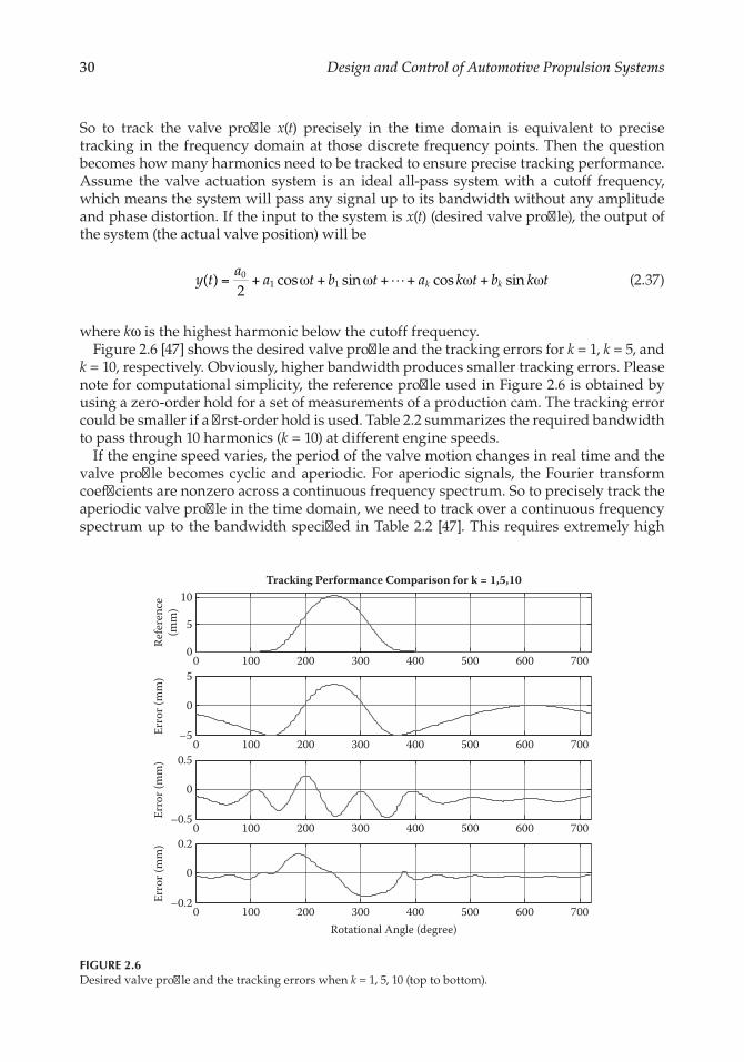
30 Design and Control of Automotive Propulsion Systems
So to track the valve profile x(t) precisely in the time domain is equivalent to precise tracking in the frequency domain at those discrete frequency points. Then the question becomes how many harmonics need to be tracked to ensure precise tracking performance. Assume the valve actuation system is an ideal all-pass system with a cutoff frequency, which means the system will pass any signal up to its bandwidth without any amplitude and phase distortion. If the input to the system is x(t) (desired valve profile), the output of the system (the actual valve position) will be
�y ta
a t b t a k t b k tk k( )2
cos sin cos sin01 1= + ω + ω + + ω + ω (2.37)
where kω is the highest harmonic below the cutoff frequency.Figure 2.6 [47] shows the desired valve profile and the tracking errors for k = 1, k = 5, and
k = 10, respectively. Obviously, higher bandwidth produces smaller tracking errors. Please note for computational simplicity, the reference profile used in Figure 2.6 is obtained by using a zero-order hold for a set of measurements of a production cam. The tracking error could be smaller if a first-order hold is used. Table 2.2 summarizes the required bandwidth to pass through 10 harmonics (k = 10) at different engine speeds.
If the engine speed varies, the period of the valve motion changes in real time and the valve profile becomes cyclic and aperiodic. For aperiodic signals, the Fourier transform coefficients are nonzero across a continuous frequency spectrum. So to precisely track the aperiodic valve profile in the time domain, we need to track over a continuous frequency spectrum up to the bandwidth specified in Table 2.2 [47]. This requires extremely high
0 100 200 300 400 500 600 7000
5
10Tracking Performance Comparison for k = 1,5,10
Refe
renc
e(m
m)
0 100 200 300 400 500 600 700–5
0
5
Erro
r (m
m)
0 100 200 300 400 500 600 700–0.5
0
0.5
Erro
r (m
m)
0 100 200 300 400 500 600 700–0.2
0
0.2
Erro
r (m
m)
Rotational Angle (degree)
FIGURE 2.6Desired valve profile and the tracking errors when k = 1, 5, 10 (top to bottom).
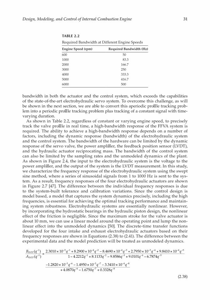
31Design, Modeling, and Control of Internal Combustion Engine
bandwidth in both the actuator and the control system, which exceeds the capabilities of the state-of-the-art electrohydraulic servo system. To overcome this challenge, as will be shown in the next section, we are able to convert this aperiodic profile tracking prob-lem into a periodic profile tracking problem plus tracking of a constant signal with time- varying duration.
As shown in Table 2.2, regardless of constant or varying engine speed, to precisely track the valve profile in real time, a high-bandwidth response of the FFVA system is required. The ability to achieve a high-bandwidth response depends on a number of factors, including the dynamic response (bandwidth) of the electrohydraulic system and the control system. The bandwidth of the hardware can be limited by the dynamic response of the servo valve, the power amplifier, the feedback position sensor (LVDT), and the hydraulic actuator reciprocating mass. The bandwidth of the control system can also be limited by the sampling rates and the unmodeled dynamics of the plant. As shown in Figure 2.4, the input to the electrohydraulic system is the voltage to the power amplifier, and the output of the system is the LVDT measurement. In this study, we characterize the frequency response of the electrohydraulic system using the swept sine method, where a series of sinusoidal signals from 1 to 1000 Hz is sent to the sys-tem. As a result, frequency responses of the four electrohydraulic actuators are shown in Figure 2.7 [47]. The difference between the individual frequency responses is due to the system-built tolerance and calibration variations. Since the control design is model based, a model that captures the system dynamics precisely, including the high frequencies, is essential for achieving the optimal tracking performance and maintain-ing system robustness. Electrohydraulic systems are essentially nonlinear. However, by incorporating the hydrostatic bearings in the hydraulic piston design, the nonlinear effect of the friction is negligible. Since the maximum stroke for the valve actuator is about 10 mm, we can use a linear model around the operating point and lump the non-linear effect into the unmodeled dynamics [50]. The discrete-time transfer functions developed for the four intake and exhaust electrohydraulic actuators based on their frequency responses are shown in Equations (2.38) to (2.41). The difference between the experimental data and the model prediction will be treated as unmodeled dynamics.
( )( )
2.3010 10 8.2900 10 8.4690 10 2.7950 10 9.8410 101 4.2212 8.1133 9.8586 9.0101 6.7874
1.2820 10 1.4950 10 3.3410 104.0870 1.6750 0.3328
1
1
5 1 4 2 4 3 3 4 4 5
1 2 3 4 5
3 6 3 7 4 8
6 7 8
B qA q
q q q q qq q q q q
q q qq q q
INTF
INTF=
× + × − × + × + ×− + − + −
− × − × − ×+ − +
−
−
− − − − − − − − − −
− − − − −
− − − − − −
− − −
(2.38)
TABLE 2.2
Required Bandwidth at Different Engine Speeds
Engine Speed (rpm) Required Bandwidth (Hz)
600 501000 83.32000 166.73000 2504000 333.35000 416.76000 500
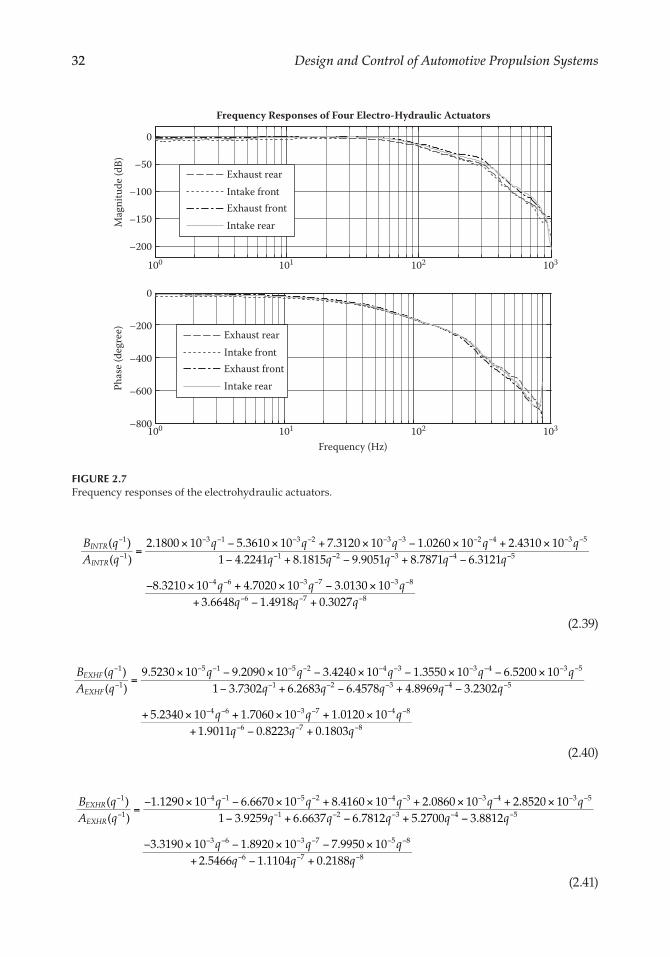
32 Design and Control of Automotive Propulsion Systems
( )( )
2.1800 10 5.3610 10 7.3120 10 1.0260 10 2.4310 101 4.2241 8.1815 9.9051 8.7871 6.3121
8.3210 10 4.7020 10 3.0130 103.6648 1.4918 0.3027
1
1
3 1 3 2 3 3 2 4 3 5
1 2 3 4 5
4 6 3 7 3 8
6 7 8
B qA q
q q q q qq q q q q
q q qq q q
INTR
INTR=
× − × + × − × + ×− + − + −
− × + × − ×+ − +
−
−
− − − − − − − − − −
− − − − −
− − − − − −
− − −
(2.39)
( )( )
9.5230 10 9.2090 10 3.4240 10 1.3550 10 6.5200 101 3.7302 6.2683 6.4578 4.8969 3.2302
5.2340 10 1.7060 10 1.0120 101.9011 0.8223 0.1803
1
1
5 1 5 2 4 3 3 4 3 5
1 2 3 4 5
4 6 3 7 4 8
6 7 8
B qA q
q q q q qq q q q q
q q qq q q
EXHF
EXHF=
× − × − × − × − ×− + − + −
+ × + × + ×+ − +
−
−
− − − − − − − − − −
− − − − −
− − − − − −
− − −
(2.40)
( )( )
1.1290 10 6.6670 10 8.4160 10 2.0860 10 2.8520 101 3.9259 6.6637 6.7812 5.2700 3.8812
3.3190 10 1.8920 10 7.9950 102.5466 1.1104 0.2188
1
1
4 1 5 2 4 3 3 4 3 5
1 2 3 4 5
3 6 3 7 5 8
6 7 8
B qA q
q q q q qq q q q q
q q qq q q
EXHR
EXHR=− × − × + × + × + ×
− + − + −
− × − × − ×+ − +
−
−
− − − − − − − − − −
− − − − −
− − − − − −
− − −
(2.41)
100 101 102 103
100 101 102 103
–200
–150
–100
–50
0
Mag
nitu
de (d
B)Frequency Responses of Four Electro-Hydraulic Actuators
Exhaust rearIntake frontExhaust frontIntake rear
–800
–600
–400
–200
0
Frequency (Hz)
Phas
e (de
gree
)
Exhaust rearIntake frontExhaust frontIntake rear
FIGURE 2.7Frequency responses of the electrohydraulic actuators.
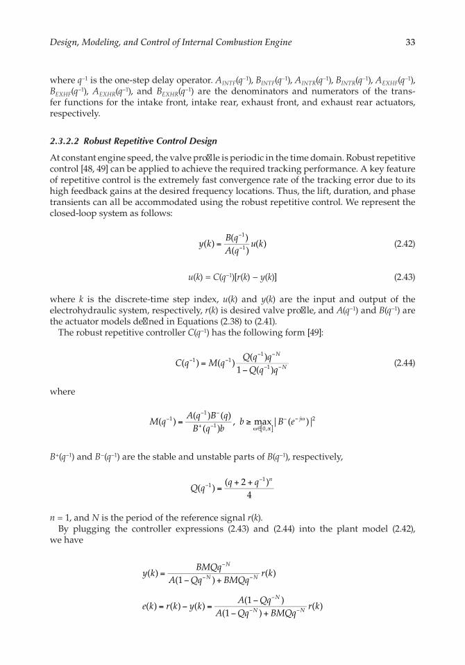
33Design, Modeling, and Control of Internal Combustion Engine
where q−1 is the one-step delay operator. AINTF(q−1), BINTF(q−1), AINTR(q−1), BINTR(q−1), AEXHF(q−1), BEXHF(q−1), AEXHR(q−1), and BEXHR(q−1) are the denominators and numerators of the trans-fer functions for the intake front, intake rear, exhaust front, and exhaust rear actuators, respectively.
2.3.2.2 Robust Repetitive Control Design
At constant engine speed, the valve profile is periodic in the time domain. Robust repetitive control [48, 49] can be applied to achieve the required tracking performance. A key feature of repetitive control is the extremely fast convergence rate of the tracking error due to its high feedback gains at the desired frequency locations. Thus, the lift, duration, and phase transients can all be accommodated using the robust repetitive control. We represent the closed-loop system as follows:
y kB qA q
u k=−
−( )( )( )
( )1
1 (2.42)
u(k) = C(q−1)[r(k) − y(k)] (2.43)
where k is the discrete-time step index, u(k) and y(k) are the input and output of the electrohydraulic system, respectively, r(k) is desired valve profile, and A(q−1) and B(q−1) are the actuator models defined in Equations (2.38) to (2.41).
The robust repetitive controller C(q−1) has the following form [49]:
( ) ( )( )
1 ( )1 1
1
1C q M qQ q q
Q q q
N
N=−
− −− −
− − (2.44)
where
M q
A q B qB q b
b B e j= ≥[ ]
−− −
+ − ω∈ π
− − ω( )( ) ( )
( ), max| ( )|1
1
1 0,
2
B+(q−1) and B−(q−1) are the stable and unstable parts of B(q−1), respectively,
( )
( 2 )4
11
Q qq q n
=+ +−
−
n = 1, and N is the period of the reference signal r(k).By plugging the controller expressions (2.43) and (2.44) into the plant model (2.42),
we have
( )(1 )
( )
( ) ( ) ( )(1 )
(1 )( )
y kBMQq
A Qq BMQqr k
e k r k y kA Qq
A Qq BMQqr k
N
N N
N
N N
=− +
= − =−
− +
−
− −
−
− −

34 Design and Control of Automotive Propulsion Systems
Since the desired valve profile r(k) is periodic with period N, we have (1−q−N)r(k) = 0, so lim ( ) 0e kk
=→∞
if Q = 1.
To accommodate the plant unmodeled dynamics and ensure robust stability, we need to compromise between tracking performance and system robustness. Define the unmodeled dynamics as
eG e G e
G ejw
jw jw
jw=−−
− −
−( )( ) ( )
( )0
0 (2.45)
where G0(e−jw) is the nominal plant model defined in (2.42) and G(e−jw) is the experimental data obtained from frequency response.
The Q filter defined in (2.44) needs to satisfy the following condition [49] to ensure system robust stability:
e
Q ejwjw1
| ( )|| ( )|≥−
− (2.46)
Frequency responses of Q(e−jw) and 1/Δ(e−jw) for the exhaust front actuator are shown in Figure 2.8 [47]; clearly condition (2.46) is satisfied. To illustrate system performance, Figure 2.9 [47] shows the frequency response of the sensitivity function of e(k) with respect to r(k) for the exhaust front actuator with closed-loop control. The notches at those harmon-ics indicate the corresponding tracking performance. For example, if a 10 Hz sine wave with amplitude 1 is applied to the system, the tracking error would be around 0.0001778. Also, as it is shown, the notch becomes smaller when it moves to the high-frequency range, which illustrates the trade-off between performance and robustness.
When engine speed varies, the period of the valve motion changes in real time. This phenomenon poses a fundamental challenge to the control design for achieving precise tracking. Some advanced control algorithms such as repetitive control cannot be applied
100 101 102 103–20
–15
–10
–5
0
5
10
15
20
25
Frequency (Hz)
Mag
nitu
de (d
B)
Q �lterInverse of unmodeled dynamics
FIGURE 2.8Frequency responses of the Q filter and the inverse of unmodeled dynamics for the exhaust front actuator.
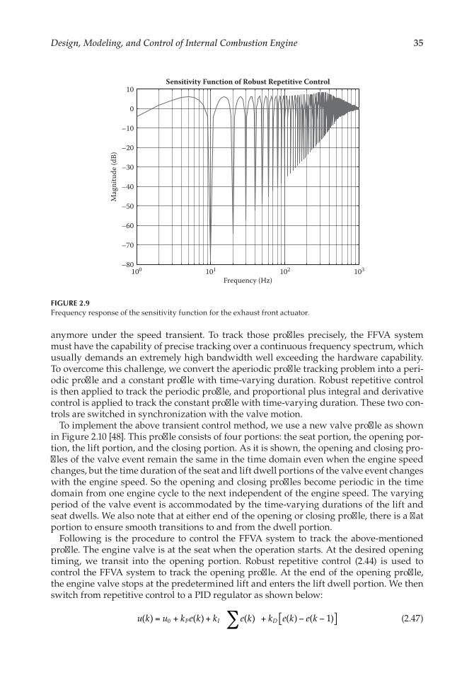
35Design, Modeling, and Control of Internal Combustion Engine
anymore under the speed transient. To track those profiles precisely, the FFVA system must have the capability of precise tracking over a continuous frequency spectrum, which usually demands an extremely high bandwidth well exceeding the hardware capability. To overcome this challenge, we convert the aperiodic profile tracking problem into a peri-odic profile and a constant profile with time-varying duration. Robust repetitive control is then applied to track the periodic profile, and proportional plus integral and derivative control is applied to track the constant profile with time-varying duration. These two con-trols are switched in synchronization with the valve motion.
To implement the above transient control method, we use a new valve profile as shown in Figure 2.10 [48]. This profile consists of four portions: the seat portion, the opening por-tion, the lift portion, and the closing portion. As it is shown, the opening and closing pro-files of the valve event remain the same in the time domain even when the engine speed changes, but the time duration of the seat and lift dwell portions of the valve event changes with the engine speed. So the opening and closing profiles become periodic in the time domain from one engine cycle to the next independent of the engine speed. The varying period of the valve event is accommodated by the time-varying durations of the lift and seat dwells. We also note that at either end of the opening or closing profile, there is a flat portion to ensure smooth transitions to and from the dwell portion.
Following is the procedure to control the FFVA system to track the above-mentioned profile. The engine valve is at the seat when the operation starts. At the desired opening timing, we transit into the opening portion. Robust repetitive control (2.44) is used to control the FFVA system to track the opening profile. At the end of the opening profile, the engine valve stops at the predetermined lift and enters the lift dwell portion. We then switch from repetitive control to a PID regulator as shown below:
u k u k e k k e k k e k e kP I D∑ [ ]= + + + − −( ) ( ) ( ) ( ) ( 1)0 (2.47)
–80
–70
–60
–50
–40
–30
–20
–10
0
10
Mag
nitu
de (d
B)
Sensitivity Function of Robust Repetitive Control
100 101 102 103
Frequency (Hz)
FIGURE 2.9Frequency response of the sensitivity function for the exhaust front actuator.

36 Design and Control of Automotive Propulsion Systems
where u0 is the initial value and kP, kI, and kD are the proportional, integral, and derivative gains, respectively.
At the desired closing timing, we transit from lift dwell into closing portion. The control system is switched back to the repetitive controller (2.44) from the PID regulator (2.47) to track the closing profile. At the end of the closing portion, the engine valve reaches the seat and enters the seat dwell portion. We switch again the feedback control to the PID regulator.
The above procedure repeats itself for the next valve event regardless of engine speed. The key advantage of the proposed control method is that it provides a unified framework to control the FFVA systems and similar applications for constant or varying engine speed. Another advantage is that the system in fully flexible in terms of lift, phasing, and duration even during the speed transient operation. The underlying principle of the control algorithm is that it converts the control problem from tracking over a continuous frequency spectrum to the tracking at discrete frequency points. Alternatively the recently developed time-varying internal model-based controller [51] can be applied to directly track the time-varying reference signal.
2.3.2.3 Experimental Results
Following are the experimental results for lift, duration, phase, speed, and mode transients.
Lift transient: As shown in Figure 2.11 [47], the desired valve lift was changed from 5.5 to 3 mm after cycle 1, and the FFVA system was able to respond to the change immediately. The maximum tracking error during cycle 2 is about 0.6 mm. The tracking error reduces to less than 0.05 mm at cycle 3. In other words, it takes
Lift Dwell
ClosingPro�le
OpeningPro�le
mm
10
9
8
7
6
5
4
3
2
1
00 0.02 0.04 0.06 0.08 0.10
Time (s)0.12 0.14 0.16 0.18 0.2
11
1000 rpm
Seat
2000 rpm
FIGURE 2.10New valve profile at 1000 and 2000 rpm engine speed.

37Design, Modeling, and Control of Internal Combustion Engine
only two engine cycles for the transient tracking errors to disappear in the case of a step lift change. Please note that the position signal shown in the figure is the position of the hydraulic piston instead of the engine valve due to the specific location of the sensor (see Figure 2.4). When the position signal is positive, the hydraulic piston and the engine valve are moving together. When the position signal becomes negative, the hydraulic piston separates from the engine valve and continues to retract while the engine valve stops at the valve seat. It is also worth pointing out that the measured position signal itself has a 0.02 mm noise level, so the steady-state tracking errors after the lift transient are mainly due to the position sensor noise.
Duration transient: A step change of 15° in valve duration was tested. As shown in Figure 2.12 [47], the duration of the valve event is increased by 15° in one step in the desired valve profile, and the actual valve position was able to follow the command in the next cycle. The tracking error converges to less than 0.2 mm in two cycles.
Phase transient: A step change of 15° in valve phasing was tested. As shown in Figure 2.13 [47], the phasing of the valve event is advanced by 15° in one step in the desired valve profile, and the actual valve position was able to follow the command in the next cycle. The tracking error converges to less than 0.3 mm in three cycles.
Speed transient: Both bench and combustion tests were conducted to test the FFVA system’s speed transient capability. Figure 2.14 [47] shows the bench test results where the FFVA system was running on the engine head without combustion and the engine encoder signal was generated by a simulator. The engine speed was changed from about 1000 to 2000 rpm. The FFVA system was able to adjust the valve event automatically in real time to accommodate the speed transient. Figure 2.15 [47] shows the combustion testing results where HCCI combustion was
0 50 100 150 200 250 300 350
0
2
4
6Lift Transient
Lift
(mm
)
0 100 200 300 400 500 600
–0.5
0
0.5
Trac
king
Err
or (m
m)
Time (ms)
Desired valve pro�leActual valve position
FIGURE 2.11Transient performance of variable lift control.
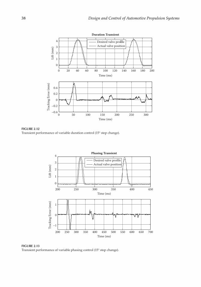
38 Design and Control of Automotive Propulsion Systems
0 20 40 60 80 100 120 140 160 180 2000
1
2
3
4
Duration Transient
Lift
(mm
)
Time (ms)
Desired valve pro�leActual valve position
0 50 100 150 200 250 300–0.4
–0.2
0
0.2
0.4
Trac
king
Err
or (m
m)
Time (ms)
FIGURE 2.12Transient performance of variable duration control (15° step change).
200 250 300 350 400 450
0
1
2
3
4Phasing Transient
Lift
(mm
)
Time (ms)
Desired valve profileActual valve position
200 250 300 350 400 450 500 550 600 650 700
–1
0
1
Trac
king
Err
or (m
m)
Time (ms)
FIGURE 2.13Transient performance of variable phasing control (15° step change).
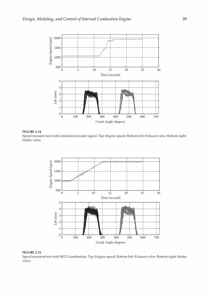
39Design, Modeling, and Control of Internal Combustion Engine
0 5 10 15 20 25 30500
1000
1500
2000
Engi
ne S
peed
(rpm
)
Time (second)
0 100 200 300 400 500 600 7000
1
2
3
4
5
Lift
(mm
)
Crank Angle (degree)
FIGURE 2.14Speed transient test with simulated encoder signal. Top: Engine speed. Bottom left: Exhaust valve. Bottom right: Intake valve.
0 5 10 15 20 25 30500
1000
1500
2000
Engi
ne S
peed
(rpm
)
Time (second)
0 100 200 300 400 500 600 7000
1
2
3
4
5
Lift
(mm
)
Crank Angle (degree)
FIGURE 2.15Speed transient test with HCCI combustion. Top: Engine speed. Bottom left: Exhaust valve. Bottom right: Intake valve.

40 Design and Control of Automotive Propulsion Systems
conducted during the speed transient and the encoder signal was generated from the encoder sensor on the crankshaft. Again, the FFVA system was able to adjust the valve event in real time based on the engine speed.
Mode transient: Mode transient was tested to accommodate combustion mode switch between HCCI and spark ignition (SI) operations. Figure 2.16 [47] shows the valve strategy change in real time between the recompression valve strategy and the nonthrottling load control valve strategy. The exhaust valve changed from 4 mm to about 8 mm with a wider duration. The intake valve advanced about 50°. We would like to point out that it is important to have precise tracking to perform such a mode transient since the engine valves could get very close to the piston during the transient.
2.4 Fuel Injection Systems
As discussed in Section 2.2, there are two kinds of fuel systems for a gasoline engine: PFI and DI fuel systems. The control aspect of both PFI and DI systems will be discussed in this subsection.
2.4.1 Fuel Injector Design and Optimization
This subsection mainly addresses the DI fuel system design and optimization.
0 100 200 300 400 500 600 7000
1
2
3
4
5
6
7
8
9
10Valve Strategy Transition
Crank Angle (Degree)
Lift
(mm
)
FIGURE 2.16Valve strategy transition between recompression and nonthrottling load control. Left: Exhaust valve. Right: Intake valve.
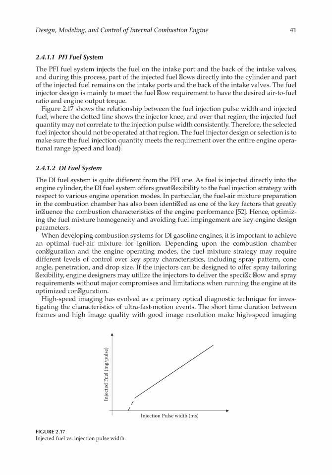
41Design, Modeling, and Control of Internal Combustion Engine
2.4.1.1 PFI Fuel System
The PFI fuel system injects the fuel on the intake port and the back of the intake valves, and during this process, part of the injected fuel flows directly into the cylinder and part of the injected fuel remains on the intake ports and the back of the intake valves. The fuel injector design is mainly to meet the fuel flow requirement to have the desired air-to-fuel ratio and engine output torque.
Figure 2.17 shows the relationship between the fuel injection pulse width and injected fuel, where the dotted line shows the injector knee, and over that region, the injected fuel quantity may not correlate to the injection pulse width consistently. Therefore, the selected fuel injector should not be operated at that region. The fuel injector design or selection is to make sure the fuel injection quantity meets the requirement over the entire engine opera-tional range (speed and load).
2.4.1.2 DI Fuel System
The DI fuel system is quite different from the PFI one. As fuel is injected directly into the engine cylinder, the DI fuel system offers great flexibility to the fuel injection strategy with respect to various engine operation modes. In particular, the fuel-air mixture preparation in the combustion chamber has also been identified as one of the key factors that greatly influence the combustion characteristics of the engine performance [52]. Hence, optimiz-ing the fuel mixture homogeneity and avoiding fuel impingement are key engine design parameters.
When developing combustion systems for DI gasoline engines, it is important to achieve an optimal fuel-air mixture for ignition. Depending upon the combustion chamber configuration and the engine operating modes, the fuel mixture strategy may require different levels of control over key spray characteristics, including spray pattern, cone angle, penetration, and drop size. If the injectors can be designed to offer spray tailoring flexibility, engine designers may utilize the injectors to deliver the specific flow and spray requirements without major compromises and limitations when running the engine at its optimized configuration.
High-speed imaging has evolved as a primary optical diagnostic technique for inves-tigating the characteristics of ultra-fast-motion events. The short time duration between frames and high image quality with good image resolution make high-speed imaging
Injection Pulse width (ms)
Inje
cted
Fue
l (m
g/pu
lse)
FIGURE 2.17Injected fuel vs. injection pulse width.
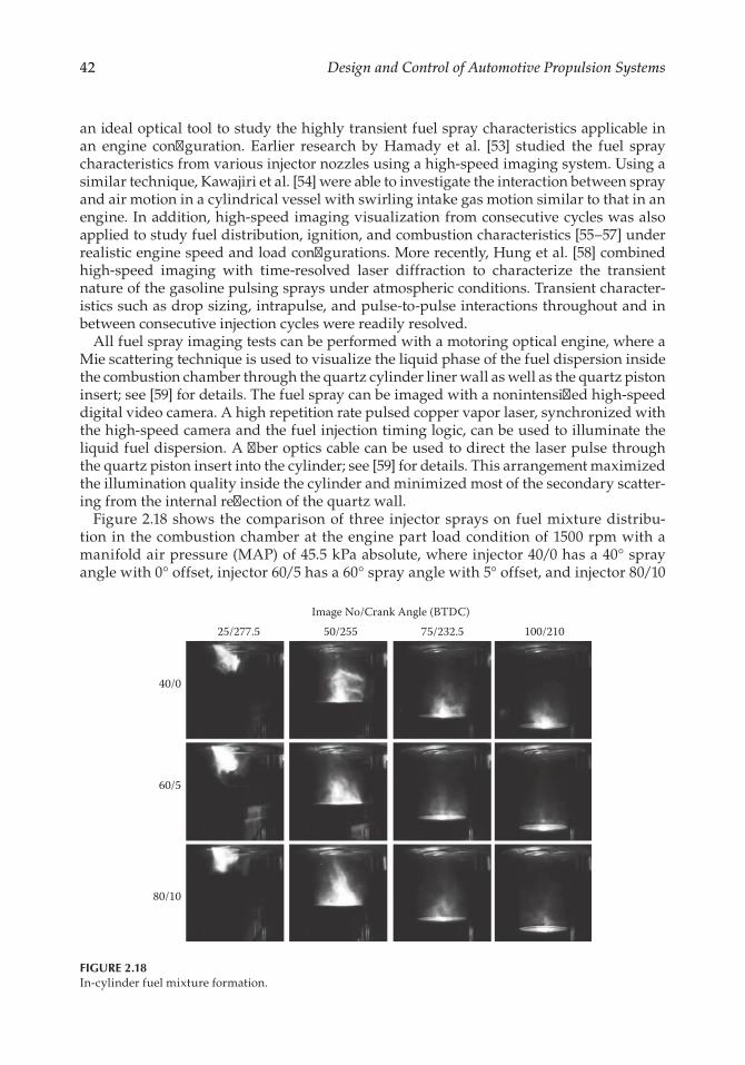
42 Design and Control of Automotive Propulsion Systems
an ideal optical tool to study the highly transient fuel spray characteristics applicable in an engine configuration. Earlier research by Hamady et al. [53] studied the fuel spray characteristics from various injector nozzles using a high-speed imaging system. Using a similar technique, Kawajiri et al. [54] were able to investigate the interaction between spray and air motion in a cylindrical vessel with swirling intake gas motion similar to that in an engine. In addition, high-speed imaging visualization from consecutive cycles was also applied to study fuel distribution, ignition, and combustion characteristics [55–57] under realistic engine speed and load configurations. More recently, Hung et al. [58] combined high-speed imaging with time-resolved laser diffraction to characterize the transient nature of the gasoline pulsing sprays under atmospheric conditions. Transient character-istics such as drop sizing, intrapulse, and pulse-to-pulse interactions throughout and in between consecutive injection cycles were readily resolved.
All fuel spray imaging tests can be performed with a motoring optical engine, where a Mie scattering technique is used to visualize the liquid phase of the fuel dispersion inside the combustion chamber through the quartz cylinder liner wall as well as the quartz piston insert; see [59] for details. The fuel spray can be imaged with a nonintensified high-speed digital video camera. A high repetition rate pulsed copper vapor laser, synchronized with the high-speed camera and the fuel injection timing logic, can be used to illuminate the liquid fuel dispersion. A fiber optics cable can be used to direct the laser pulse through the quartz piston insert into the cylinder; see [59] for details. This arrangement maximized the illumination quality inside the cylinder and minimized most of the secondary scatter-ing from the internal reflection of the quartz wall.
Figure 2.18 shows the comparison of three injector sprays on fuel mixture distribu-tion in the combustion chamber at the engine part load condition of 1500 rpm with a manifold air pressure (MAP) of 45.5 kPa absolute, where injector 40/0 has a 40° spray angle with 0° offset, injector 60/5 has a 60° spray angle with 5° offset, and injector 80/10
40/0
60/5
80/10
Image No/Crank Angle (BTDC)25/277.5 50/255 75/232.5 100/210
FIGURE 2.18In-cylinder fuel mixture formation.

43Design, Modeling, and Control of Internal Combustion Engine
has an 80° spray angle with 10° offset. The start of injection (SOI) was set at 300° crank angle (CA) before top dead center (BTDC). With the adjusted cam phasing timing, the intake valve was lifted to about 8 mm at this SOI. The injection pulse width (duration) was set to correspond to lambda equal to 1 (stoichiometric) condition. These images were recorded within an injection cycle at different crank degrees. It is worth mention-ing that the injector driver has 1 ms precharge delay, and so it corresponded to the delay of either 9 CAD/ms (at 1500 rpm) or 15 CAD/ms (at 2500 rpm) before the fuel spray was observed at the top of the cylinder. Note that the precharge delay definition can be found in Figure 2.22. The first image of the sequence was shown at 277.5° BTDC, where the initial portion of the spray entering the cylinder was found to be about the same for all three sprays. The intake air did not have much effect on the beginning of the spray. The narrow spray of 40/0 showed a slightly stronger axial penetration along the injector axis into the cylinder. At 255° BTDC, the fuel charge started to show some noticeable differences in the fuel distribution. The 40/0 spray penetrated more directly across the cylinder toward the liner wall, while the 60/5 and 80/10 sprays were mov-ing more toward the central region of the cylinder. They produced very minimal fuel impingement on the opposite side of the liner wall. It also shows that at this SOI timing, the leading portion of the sprays impinged slightly on the piston top. However, as the cycle progressed to 210° BTDC, the fuel distributions among all three sprays were quite similar.
Based on the distinct features depicted in Figure 2.19, it is possible to identify and extract more information on the mixture formation from these images with image processing. Therefore, image processing algorithms were developed in [59] to measure the semiquan-titative information, such as the magnitude of fuel spray impingement on cylinder wall and piston top, and fuel-air mixture homogeneity.
For example, to analyze the fuel impingement magnitude on the cylinder wall, a fuel impingement index on the cylinder wall can be defined based upon the illumination intensity of the location (pixel) on the image near the cylinder wall. The methodol-ogy of the fuel impingement on the cylinder wall is briefly outlined below. Figure 2.20
FIGURE 2.19Location of the fuel impingement analysis (illustrated by the measurement region). Left: 40/0 spray. Right: 80/10 spray.

44 Design and Control of Automotive Propulsion Systems
depicts the measurement areas shown as a gray bar along the cylinder wall where the illumination intensity of each pixel in the image is extracted. The size of this area depends on the image orientation and measurement location of interest. For the analysis of fuel impingement on the cylinder wall, a thin area band was chosen to be 5 pixels (ith) wide by 300 pixels (jth) long. Then, an average intensity is computed by averaging the pixel intensity across the width (i.e., across the ith direction) of the area at each jth pixel as follows:
,
,
1I
I
Nave j
i j
i
N
∑= = (2.48)
where Ii,j is the intensity of an individual pixel in the measurement area. N is number of pixels along the width, and it is equal to 5 for this analysis.
Figure 2.20 shows the comparison of the average intensity between the two spray patterns along the measurement line. For both sprays, there was no fuel impingement near the top of the cylinder wall. However, it can be seen that for the 40/0 spray, the average intensity along the cylinder wall started to increase abruptly at about one-third of the stroke distance, and it peaked at about halfway on the cylinder. After the peak, the intensity continued to decrease toward the bottom of the cylinder. Fuel impingement was found to spread more on the lower half of the cylinder wall. Conversely, for the wider spray of 80/10, there was almost no impingement of fuel along the cylinder wall. The average intensity remained very minimal and constant along the entire analysis location.
Since the fuel impingement is strongly transient and it is rapidly changing at different crank angles within an engine cycle, an overall fuel impingement index (FII) at a specific
0
5
10
15
20
25
30
35
40Av
erag
e Pix
el In
tens
ity (a
.u.)
Test 55 (40 deg spray anglewith zero o�set angle)Test 87 (80 deg spray anglewith 10 deg o�set angle)
Top of Analysis Location Bottom of Analysis Location
FIGURE 2.20Comparison of ensemble average intensity on wall impingement when piston is at bottom dead center (BDC).

45Design, Modeling, and Control of Internal Combustion Engine
crank angle can also be defined based on the ensemble average intensity over the entire location along the jth direction of the measurement domain:
,
1FII
I
MCA
ave j
j
M
∑= = (2.49)
where M is the number of pixels along the length of the measurement domain and M is equal to 300 for this analysis. This index can be used to track and analyze the extent of fuel impingement at each crank angle degree over the injection cycle. Figure 2.21 shows such a plot of crank angle-resolved fuel impingement index on the cylinder wall. This figure also reveals several useful facts about characteristics such as the sequence and the duration of the fuel impingement. The injection logic pulse started at 270° BTDC when the image sequence was commenced. Taking the injector driver precharge delay into account, the fuel spray entered the cylinder at about 246° BTDC. The spray then propa-gated directly across the cylinder and started to impinge on the cylinder wall at about 210° BTDC. The impingement index started to increase as the piston continued to sweep down-ward. For both sprays, even though the peak of impingement was observed to be between 140° and 130° BTDC, the narrow spray with 40/0 resulted in substantially higher cylinder wall impingement than the wider spray of 80/10. Impingement continued to decrease for both sprays as the piston reached about 100° BTDC. Beyond this crank angle, the fuel impingement for both sprays was found to be very minimal.
Similar to any other image analysis methods based on light intensity extracted from the pixels of an image, it is important to realize that the fuel impingement analysis technique mentioned above also requires a consistent light illumination and background in the region
Cylinder Wall Fuel Impingement Index 2500 RPM/WOT
0.0
5.0
10.0
15.0
20.0
25.0
30.0
50100150200250300Degrees CA (BTDC)
Fuel
Impi
ngem
ent I
ndex
(a.u
.)
40° spray angle with0° o�set angle80° spray angle with10° o�set angle
Spray Enters Cylinder
ImpingementBegins
FIGURE 2.21Crank angle resolved fuel impingement index on cylinder liner wall.

46 Design and Control of Automotive Propulsion Systems
of interest in order to minimize any possible inaccuracy or uncertainty. For example, any fuel droplets populated in the bottom of the liner wall or in the shadow of the piston quartz insert may not be accounted for equally due to the uneven light intensity distribu-tion inside the cylinder. In addition, any residual fuel left behind from previous cycles may remain in the cylinder or be deposited on the walls as the cycle progresses. This could potentially overestimate the quantity and location of the fuel impingement at a particular crank angle. Therefore, a proper background subtraction may be needed to eliminate any contribution of the residual fuel from previous cycles.
Even though this fuel impingement index cannot be used directly to correlate the amount of fuel impinged on the wall, this value indicates the extent as well as the loca-tion of the fuel impingement at a specific crank angle within a cycle. Since it is based on the illumination intensity of the pixel, once the images are properly adjusted to correct for any illumination deviation in the imaging setup, it may be useful for comparing other fuel mixing qualities between different conditions.
As a summary, high-speed imaging can be performed to visualize the spray pattern effect on fuel mixture formation as a function of crank angle in a single-cylinder engine for direct injection gasoline applications. With the use of the imaging diagnostics to dif-ferentiate the fuel mixing characteristics produced by three different spray patterns, it was found that the spray angle, offset angle, and injector mounting orientation had pro-nounced effects on the fuel mixture preparation. The fuel mixture inside the combustion chamber was affected more by the spray pattern at full load than on part load condition.
Fuel impingement on cylinder liner walls can also be investigated by using image processing and analysis algorithms. Using high-speed imaging, the transient nature of fuel impingement was resolved as a function of crank angle degree. If a consistent light intensity through the image was ensured, the location and extent of fuel impingement of various spray patterns could be differentiated and compared. Similar image analysis methods may also be applied to evaluate the fuel impingement on the top of the piston. A new injector spray pattern is currently being revised that will not only minimize the fuel impingement on the liner wall and intake valves, but also enhance the overall fuel distribution. These results can be used to correlate the engine combustion and emission performance in the subsequent single-cylinder dynamometer combustion testing. Detailed high-speed visualization of in-cylinder fuel spray and the associated impingement study approach can be found in [59] and [60].
2.4.2 Fuel Injector Model and Control
The fuel injector dynamics for PFI injectors is normally ignored due to relatively fast tran-sient dynamics compared to the wall-wetting dynamics. The main dynamics in the engine model is described in Section 2.2.3.
However, for DI injectors, due to the high fuel pressure, the relationship between injected fuel and commanded injection pulse width is complicated. It was apparent in [61] that there was little uniformity throughout the automotive industry in the use of the term pulse width. The lack of uniformity becomes quite important for gasoline DI injection systems, due to the fact that the pulse control strategies can be significantly more complex than those of PFI systems. Many, but not all, DI drivers incorporate a designed driver charge delay (DCD) time between the initiation of the logic pulse from the engine control unit (ECU) and the command pulse of the driver to open the injector. This is normally done to ensure a maximum voltage level of the driver capacitor just prior to actuation. The interrelationships of four key timing traces are illustrated schematically in Figure 2.22.
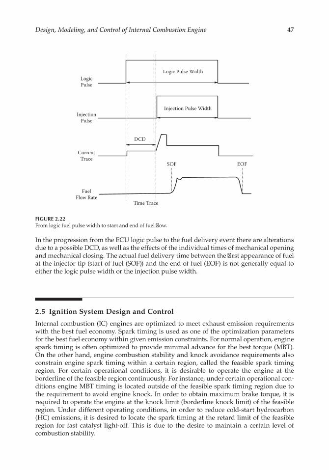
47Design, Modeling, and Control of Internal Combustion Engine
In the progression from the ECU logic pulse to the fuel delivery event there are alterations due to a possible DCD, as well as the effects of the individual times of mechanical opening and mechanical closing. The actual fuel delivery time between the first appearance of fuel at the injector tip (start of fuel (SOF)) and the end of fuel (EOF) is not generally equal to either the logic pulse width or the injection pulse width.
2.5 Ignition System Design and Control
Internal combustion (IC) engines are optimized to meet exhaust emission requirements with the best fuel economy. Spark timing is used as one of the optimization parameters for the best fuel economy within given emission constraints. For normal operation, engine spark timing is often optimized to provide minimal advance for the best torque (MBT). On the other hand, engine combustion stability and knock avoidance requirements also constrain engine spark timing within a certain region, called the feasible spark timing region. For certain operational conditions, it is desirable to operate the engine at the borderline of the feasible region continuously. For instance, under certain operational con-ditions engine MBT timing is located outside of the feasible spark timing region due to the requirement to avoid engine knock. In order to obtain maximum brake torque, it is required to operate the engine at the knock limit (borderline knock limit) of the feasible region. Under different operating conditions, in order to reduce cold-start hydrocarbon (HC) emissions, it is desired to locate the spark timing at the retard limit of the feasible region for fast catalyst light-off. This is due to the desire to maintain a certain level of combustion stability.
Logic Pulse Width
Injection Pulse Width
DCD
SOF
Time Trace
FuelFlow Rate
CurrentTrace
InjectionPulse
LogicPulse
EOF
FIGURE 2.22From logic fuel pulse width to start and end of fuel flow.

48 Design and Control of Automotive Propulsion Systems
Figure 2.23 shows a typical spark timing feasible region as a function of exhaust gas recirculation (EGR) for a desired level of combustion stability with coefficient of variation (COV) of IMEP less than 3%, where the thick dashed line represents the engine MBT spark timing, the thick dash-dot line represents the engine advanced (knock) spark limit, and the thick solid line represents the retard spark limit. It can be observed that knock, MBT, and retard limits vary as a function of EGR rate, which makes it difficult to control the optimal spark timing in an open-loop fashion. Further, this feasible region varies in shape with different engine operational and environmental conditions.
In current production applications, MBT timing is an open-loop feedforward control whose values are experimentally determined by conducting spark sweeps at different speed and load points, and at different environmental operating conditions. Almost every calibration point needs a spark sweep to see if the engine can be operated at the MBT timing condition. If not, a certain degree of safety margin is needed to avoid preignition or knock during engine operation. Open-loop spark mapping usually requires a tremendous amount of effort and time to achieve a satisfactory calibration.
Existing knock spark limit control utilizes an accelerometer-based knock sensor for feedback control. Due to the low signal-to-noise ratio, conventional approaches are based on the use of a knock flag signal obtained by comparing the knock intensity signal of a knock sensor to a given threshold. The knock intensity signal is defined as the integrated value, over a given knock window, of the absolute value signal obtained by filtering the raw knock sensor signal using a band-pass filter. This knock flag signal is the input to a dual-rate (slow and fast correction) count-up/count-down engine knock limit controller. The disadvantage of this control scheme is that it continually takes the engine in and out of knock, rather than operating continually at the desired borderline knock limit. In addition, at certain operating points knock observability can be severely compromised by engine mechanical noises such as valve closures and piston slap, which may be picked up by the accelerometer. Such issues result in conservative ignition timing that leads to reduced engine performance.
As discussed before, during a cold start, it is desirable to operate the engine at its retard spark timing limit for minimal HC emissions. The retard spark timing limit is
EGR
(%)
Advanced <----Spark Timing (DBTDC) ----> Retard22
3
3
3
2
2
2
10
10
3
3
3
5
5
5
5
MBT Timing 8
8
Knock Limit
Retard Limit
COV (IMEP)
5
FIGURE 2.23Feasible region of spark timing.

49Design, Modeling, and Control of Internal Combustion Engine
often constrained by engine combustion stability metrics such as COV of IMEP. Due to unavailability of production-ready in-cylinder pressure sensors, the retard spark timing limit is obtained through an offline engine mapping process, leading to conservative calibrations. In addition, to accommodate the range of fuels used throughout a market, this calibration is made even more conservative.
In recent years, various closed-loop spark timing control schemes have been proposed based upon in-cylinder pressure measurements [61–68] or spark ionization current sensing [69–72, 77]. Based upon test data, it has been found that the peak cylinder pressure (PCP) usually occurs around 15° after top dead center (TDC) at MBT timing [69]. The 50% mass fraction burned (MFB) point generally occurs between 8° and 10° after TDC when MBT timing is achieved. The algorithm published in [63] controls PR(10) (normalized pressure ratio of in-cylinder and motoring pressures at 10° after TDC) around 0.55 to obtain the MBT timing.
Due to recent advances in electronics technology, ionization current can be detected at 15 μA with very low background noise. The high quality of an in-cylinder ioniza-tion signal makes it possible to derive a linear knock intensity that is proportional to the knock level [74–76]. It can also be processed to derive a metric for combustion quality similar to the COV of IMEP and closeness of combustion to partial burn and misfire limit [76, 82], which can be used as a feedback signal for retard limit control. Engine MBT timing can also be derived from in-cylinder ionization signals similar to the pressure signals [63, 69]. Since MBT criteria derived from pressure and ioniza-tion signals are solely based upon observations and may change at different operating conditions, the associated control algorithms still require some dynamometer-based calibration effort. It is clear that the combustion process has to be matched with the engine cylinder volume change to attain the best torque. The major advantage for the ionization-based closed-loop MBT timing control is that no additional sensing element or assembly steps are required since it uses the spark plug as an ignition actuator and a combustion sensor.
This section proposes a closed-loop ignition control architecture (see Figure 2.24) that combines MBT timing control, knock, and retard timing limit control strategies into
SignalSampling &
Conditioning
IonSignals
Ionization DetectionIgnition Coils
KnockIntensity
Calculation
StochasticKnock Limit
Control
Closed LoopMBT Timing
Control
MBT TimingSignal
Calculation
CombustionStability
Calculation
StochasticRetard Limit
ControlIgnitionControlSignal
Generation
Spark TimingLimit
Management
PCM
FIGURE 2.24Closed-loop ignition timing control system.
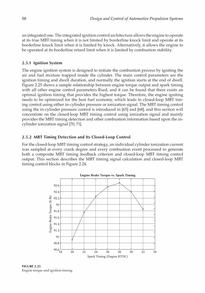
50 Design and Control of Automotive Propulsion Systems
an integrated one. The integrated ignition control architecture allows the engine to operate at its true MBT timing when it is not limited by borderline knock limit and operate at its borderline knock limit when it is limited by knock. Alternatively, it allows the engine to be operated at its borderline retard limit when it is limited by combustion stability.
2.5.1 Ignition System
The engine ignition system is designed to initiate the combustion process by igniting the air and fuel mixture trapped inside the cylinder. The main control parameters are the ignition timing and dwell duration, and normally the ignition starts at the end of dwell. Figure 2.25 shows a sample relationship between engine torque output and spark timing with all other engine control parameters fixed, and it can be found that there exists an optimal ignition timing that provides the highest torque. Therefore, the engine igniting needs to be optimized for the best fuel economy, which leads to closed-loop MBT tim-ing control using either in-cylinder pressure or ionization signal. The MBT timing control using the in-cylinder pressure control is introduced in [65] and [68], and this section will concentrate on the closed-loop MBT timing control using ionization signal and mainly provides the MBT timing detection and other combustion information based upon the in-cylinder ionization signal [70, 71].
2.5.2 MBT Timing Detection and Its Closed-Loop Control
For the closed-loop MBT timing control strategy, an individual cylinder ionization current was sampled at every crank degree and every combustion event processed to generate both a composite MBT timing feedback criterion and closed-loop MBT timing control output. This section describes the MBT timing signal calculation and closed-loop MBT timing control blocks in Figure 2.24.
18 20 22 24 26 28 30 32 3490.6
90.8
91
91.2
91.4
91.6
91.8
92
92.2
92.4
92.6
Spark Timing (Degree BTDC)
Engi
ne B
rake
Tor
que (
ft-lb
)
Engine Brake Torque vs. Spark Timing
FIGURE 2.25Engine torque and ignition timing.

51Design, Modeling, and Control of Internal Combustion Engine
2.5.2.1 Full-Range MBT Timing Detection
The MFB is determined by the well-known Rassweiler–Withrow [62] method, established in 1938, through pressure measurement. Through MFB one can find when the combustion has its peak burning velocity, acceleration, and percentage burn location as a function of crank angle. Maintaining these critical events at a specific crank angle produces the most efficient combustion process. In other words, the MBT timing can be found through these critical events. In reference [68], instead of directly using the MFB, the connection between MFB and net pressure is utilized to simplify analysis. The net pressure and its first and second derivatives are used to represent the distance, velocity, and acceleration of the combustion process. References [68] and [69] show that PCP location, 50% MFB location, and maximum acceleration location of the net pressure can each be used as MBT timing criteria for closed-loop control.
Figure 2.26 shows a typical ionization signal vs. crank angle and the corresponding in-cylinder pressure signal. Different from an in-cylinder pressure signal, an ionization signal actually shows more detailed information about the combustion process through its waveform. It shows when a flame kernel is formed and propagates away from the gap, when the combustion is accelerating rapidly, when the combustion reaches its peak burning rate, and when the combustion ends. A typical ionization signal usually consists of two peaks. The first peak of the ion signal represents the flame kernel growth and development, and the second peak is the reionization due to the in-cylinder temperature increase resulting from both pressure increase and flame development in the cylinder.
The use of an ionization signal for MBT timing detection was studied in [73]. As described in [73], the inflection point right after the first peak (called the first inflection point; see Figure 2.26) can be correlated to the maximum acceleration point of the net pressure, and this point is usually between 10% and 15% MFB. The inflection point right before
–50 0 50 100 1501.5
2
2.5
3
3.5
4
4.5
5
5.5
Crank Angle (Degree)
Ion
Volta
ge
–50 0 50 100 150
0
5
10
15
20
25
30
35
40
Pressure
Pres
sure
(Bar
)
Operational Conditions: 1500RPM, 2.62 Bar Load, 16° BTDC
Ion
2nd Peak
1st In�ection Point
2nd In�ection Point
FIGURE 2.26A typical ionization signal as function of crank angle.

52 Design and Control of Automotive Propulsion Systems
the second peak of the ionization signal (called the second inflection point; see Figure 2.26) correlates well with the maximum heat release point and is located right around the 50% MFB location. Finally, the second peak location is related to the peak pressure location of the pressure signal (see Figure 2.26).
As described in [68, 69, 71], at MBT timing the maximum acceleration point of MFB (MAMFB) is located at around TDC, the 50% MFB location (50% MFB) is between 8° and 10° after TDC, and the peak cylinder pressure location (PCPL) is around 15° after TDC. Using the MBT timing criteria relationship between in-cylinder pressure and in-cylinder ionization signal, these three MBT timing criteria (MAMFB, 50% MFB, and PCPL) can be obtained using an in-cylinder ionization signal.
It is well known that the second peak of the ionization signal is mainly due to the high in-cylinder temperature during the combustion process. In the case that in-cylinder tem-perature cannot reach the reionization temperature threshold, the second peak of the ionization signal may disappear. For example, when the engine is operated either at the idle condition, with a very high EGR rate, or with a lean air-to-fuel (A/F) mixture, or a combination of the above, the flame temperature is relatively low and the temperature could be below the reionization temperature threshold. Therefore, the second peak may not appear in the ionization signal.
Previously mentioned MBT timing correlations over the entire operating range were presented in [68, 73] and are omitted here for brevity. During this study, it was observed that the following three cases cover all the possible ionization signals over the speed and load map:
Case 1: Normal ionization waveform. Both peaks are present in the waveform.Case 2: The first peak ionization signal; low combustion temperature resulting in no
second peak.Case 3: The second peak ionization signal; high engine speed such that the first peak
merges with the ignition signal due to the relatively longer ignition duration as a result of a relatively constant spark duration at high engine speed.
Figure 2.27 shows a representative example from each of the three cases. For the case 1 example, the engine was operated at 1500 rpm with 2.62 bar brake mean effective pressure (BMEP) load and without EGR; for the case 2 example, the engine was running at the same condition as case 1, except with 15% EGR; and for the case 3 example, the engine was run-ning at 3500 rpm with wide-open throttle (WOT).
It is clear from Figure 2.27 that three MBT timing criteria (MAMFB, 50% MFB, and PCPL) are available only in case 1, and for cases 2 and 3, only one or two criteria are available. This indicates that at some operating conditions, only one or two MBT timing criteria can be obtained for MBT timing feedback. The proposed MBT timing estimation method combines all MBT timing criteria available at current operational conditions into one single composite criterion for improved reliability and robustness. The detailed algo-rithm is described in the next section.
In order to implement the MBT timing estimation strategy using an in-cylinder ion-ization signal, a detection algorithm was developed in [71]. The MBT timing detection algorithm can be divided into the following four steps:
Step 1: Ionization signal conditioning. For each given cylinder, the ionization signal is sampled at every crank degree after the ignition coil dwell event for 120°, as the ionization signal disappears after 120 crank angle degrees. The sampled
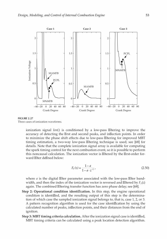
53Design, Modeling, and Control of Internal Combustion Engine
ionization signal Ion(⋅) is conditioned by a low-pass filtering to improve the accuracy of detecting the first and second peaks, and inflection points. In order to minimize the phase shift effects due to low-pass filtering for improved MBT timing estimation, a two-way low-pass filtering technique is used; see [68] for details. Note that the complete ionization signal array is available for computing the spark timing control for the next combustion event, so it is possible to perform this noncausal calculation. The ionization vector is filtered by the first-order for-ward filter defined below:
1
1,1F (z)
aa z
F =−
− ⋅ − (2.50)
where a is the digital filter parameter associated with the low-pass filter band-width, and then the index of the ionization vector is reversed and filtered by FF(z) again. The combined filtering transfer function has zero phase delay; see [68].
Step 2: Operational condition identification. In this step, the engine operational condition is identified, and the resulting output of this step is the determina-tion of which case the sampled ionization signal belongs to, that is, case 1, 2, or 3. A pattern recognition algorithm is used for the case identification by using the calculated number of peaks, inflection points, and their distances from the end of ignition.
Step 3: MBT timing criteria calculation. After the ionization signal case is identified, MBT timing criteria can be calculated using a peak location detection algorithm.
–40–20 0 20 40 60 80
0
0.5
1
1.5
2
Ioni
zatio
n Vo
ltage
Crank Degree
Case 1
–40–20 0 20 40 60 80
0
0.5
1
1.5
2
Crank Degree
Case 2
–40 –20 0 20 40 60 80
0
0.5
1
1.5
2
Crank Degree
Case 3
MAMFB
MAMFB
PCPL
PCPL
50%MFB
50%MFB
FIGURE 2.27Three cases of ionization waveforms.
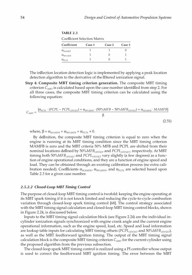
54 Design and Control of Automotive Propulsion Systems
The inflection location detection logic is implemented by applying a peak location detection algorithm to the derivative of the filtered ionization signal.
Step 4: Composite MBT timing criterion generation. The composite MBT timing criterion CMBT is calculated based upon the case number identified from step 2. For all three cases, the composite MBT timing criterion can be calculated using the following equation:
CMBT =[αPCPL ⋅ (PCPL − PCPLOFFSET) + α50%MFB ⋅ (50%MFB − 50%MFBOFFSET) + αMAMFB ⋅ MAMFB]
β
(2.51)
where, β = αMAMFB + α50%MFB + αPCPL ≠ 0. By definition, the composite MBT timing criterion is equal to zero when the
engine is running at its MBT timing condition since the MBT timing criterion MAMFB is zero and the MBT criteria 50% MFB and PCPL are shifted from their nominal locations defined by 50%MFBOFFSET and PCPLOFFSET , respectively. At MBT timing both 50%MFBOFFSET and PCPLOFFSET vary slightly (a few degrees) as a func-tion of engine operational conditions, and they are a function of engine speed and load. They can be obtained through an existing calibration process (no extra cali-bration needed). Coefficients αMAMFB , α50%MFB , and αPCPL are selected based upon Table 2.3 for a given case number.
2.5.2.2 Closed-Loop MBT Timing Control
The purpose of closed-loop MBT timing control is twofold: keeping the engine operating at its MBT spark timing if it is not knock limited and reducing the cycle-to-cycle combustion variation through closed-loop spark timing control [68]. The control strategy associated with the MBT timing signal calculation and closed-loop MBT timing control blocks, shown in Figure 2.24, is discussed below.
Inputs to the MBT timing signal calculation block (see Figure 2.24) are the individual in-cylinder ionization signals synchronized with engine crank angle and the current engine operational information, such as the engine speed, load, etc. Speed and load information are lookup table inputs for calculating MBT timing offsets (PCPLOFFSET and 50%MFBOFFSET), as well as the MBT feedforward ignition timing. The output of the MBT timing signal calculation block is the composite MBT timing criterion CMBT for the current cylinder using the proposed algorithm from the previous subsection.
The closed-loop spark MBT timing control is realized using a PI controller whose output is used to correct the feedforward MBT ignition timing. The error between the MBT
TABLE 2.3
Coefficient Selection Matrix
Coefficient Case 1 Case 2 Case 3
αMAMFB 1 1 0
α50%MFB 1 0 1
αPCPL 1 0 1
55Design, Modeling, and Control of Internal Combustion Engine
criterion reference and the composite MBT timing criterion is used as an input to the PI controller. Under the study conditions used in this work, the MBT criteria reference signal was set to zero. However, this is not necessary. For example, under certain conditions, to meet emission requirements it may be desired to retard spark timing from its MBT tim-ing by a few degrees. Under these conditions, the reference signal can be set to a negative value.
2.5.3 Stochastic Ignition Limit Estimation and Control
This section describes a stochastic ignition limit control algorithm that is used for both advanced and retard ignition timing limit controls.
2.5.3.1 Stochastic Ignition Limit Estimation
This subsection discusses how to generate a feedback measure for the retard limit con-trol, which is the functionality of the combustion stability calculation block shown in Figure 2.24. A typical ionization signal with its integration window is displayed in Figure 2.28. Before defining the combustion stability criterion, let us define an integral ratio function RINT (⋅) as follows:
R k
Ion i
Ion i
k nINTi CS
CS k
i CS
CS n
∑
∑= × ≤=
+ −
=
+ −( )
( )
( )
100%,
1
1 (2.52)
–40 –20 0 20 40 60Crank Angle (DATDC)
Ioni
zatio
n Si
gnal
and
Inte
gral
(Vol
tage
)
90% Dist. Location
90% Int. Level
IntegralIon
Int. Window
Typical Ionization Signal3.5
3
2.5
2
1.5
1
0.5
0
–0.5
FIGURE 2.28Ionization signal and integration location.

56 Design and Control of Automotive Propulsion Systems
where Ion(⋅) is a 120-element ionization vector sampled at the start of ignition with one crank degree resolution (same vector for the MBT timing estimation), CS is the crank angle index at the start of the integration window (see Figure 2.28), and n is the crank degrees representing the integration window width. The integration location (IL) of a given percentage RDES is an integer IL(RDES) that satisfies the following equation:
RINT[IL(RDES) − 1] < RDES ≤ RINT [IL(RDES)] (2.53)
Figure 2.28 shows a 90% integration location IL(90%). Note that 100% integration location IL(100%) is ideally reached at the end of the integration window.
Figure 2.29 shows the stochastic properties of IL(90%) with spark timing at 21° before TDC. Three hundred cycles (number of consecutive firing events at the same spark timing) of data are used to create the probability density function (PDF) or histogram of the inte-gration location, where the solid line is a Gaussian distribution fit of PDF data.
Based on the PDF shown in Figure 2.29, the statistics of the ionization integration loca-tions seem to be close to those of a Gaussian random process. As the spark timing becomes more retarded, the PDF of integration location starts skewing toward the retard direction (see [77] for details). But more importantly, at the spark timing with a desired combustion stability level, the PDFs are close to those of a Gaussian random process.
The mean and standard deviation of the ionization integration locations (90%) during a spark sweep at 1500 rpm with 2.62 bar BMEP are shown in Figure 2.30, where stars represent the test data and the solid lines are fitted curves using polynomials. It can be observed that both mean and standard deviation of integration location increase as the spark timing retards.
2.5.3.2 Knock Intensity Calculation and Its Stochastic Properties
This subsection is associated with the knock intensity calculation block in Figure 2.24. Under engine operational conditions that result in knock, knock intensity can be calculated
–5 0 5 10Crank Location (DATDC)
Prob
abili
ty D
ensit
y Fun
ctio
n (P
DF)
0.14
0.12
0.1
0.08
0.06
0.04
0.02
015 20 25
Gaussian �t: mean = 5.77, std = 5.11
FIGURE 2.29Ion integration location PDF.
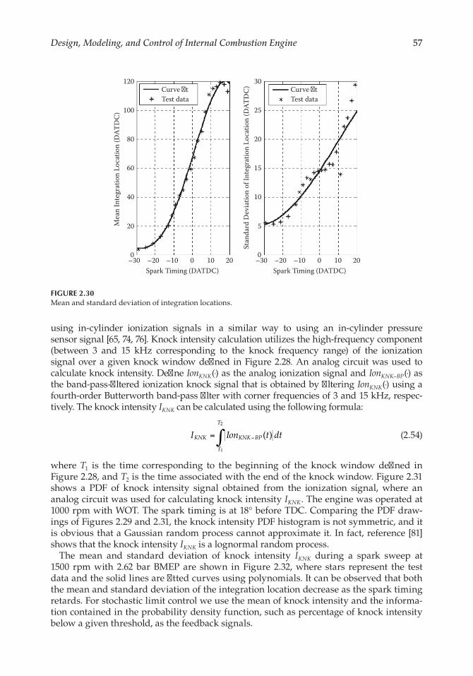
57Design, Modeling, and Control of Internal Combustion Engine
using in-cylinder ionization signals in a similar way to using an in- cylinder pressure sensor signal [65, 74, 76]. Knock intensity calculation utilizes the high- frequency component (between 3 and 15 kHz corresponding to the knock frequency range) of the ionization signal over a given knock window defined in Figure 2.28. An analog circuit was used to calculate knock intensity. Define IonKNK (⋅) as the analog ionization signal and IonKNK−BP (⋅) as the band-pass-filtered ionization knock signal that is obtained by filtering IonKNK (⋅) using a fourth-order Butterworth band-pass filter with corner frequencies of 3 and 15 kHz, respec-tively. The knock intensity IKNK can be calculated using the following formula:
( )1
2
I Ion t dtKNK KNK BP
T
T
∫= − (2.54)
where T1 is the time corresponding to the beginning of the knock window defined in Figure 2.28, and T2 is the time associated with the end of the knock window. Figure 2.31 shows a PDF of knock intensity signal obtained from the ionization signal, where an analog circuit was used for calculating knock intensity IKNK . The engine was operated at 1000 rpm with WOT. The spark timing is at 18° before TDC. Comparing the PDF draw-ings of Figures 2.29 and 2.31, the knock intensity PDF histogram is not symmetric, and it is obvious that a Gaussian random process cannot approximate it. In fact, reference [81] shows that the knock intensity IKNK is a lognormal random process.
The mean and standard deviation of knock intensity IKNK during a spark sweep at 1500 rpm with 2.62 bar BMEP are shown in Figure 2.32, where stars represent the test data and the solid lines are fitted curves using polynomials. It can be observed that both the mean and standard deviation of the integration location decrease as the spark timing retards. For stochastic limit control we use the mean of knock intensity and the informa-tion contained in the probability density function, such as percentage of knock intensity below a given threshold, as the feedback signals.
–300
–20 –10 0 10 20
20
40
60
80
100
120
Mea
n In
tegr
atio
n Lo
catio
n (D
ATD
C)
Spark Timing (DATDC)
Curve �tTest data
–300
–20 –10 0 10 20
5
10
15
20
25
30
Stan
dard
Dev
iatio
n of
Inte
grat
ion
Loca
tion
(DAT
DC
)
Spark Timing (DATDC)
Curve �tTest data
FIGURE 2.30Mean and standard deviation of integration locations.
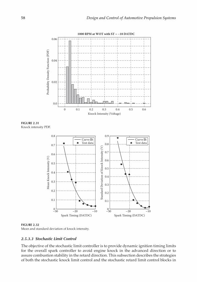
58 Design and Control of Automotive Propulsion Systems
2.5.3.3 Stochastic Limit Control
The objective of the stochastic limit controller is to provide dynamic ignition timing limits for the overall spark controller to avoid engine knock in the advanced direction or to assure combustion stability in the retard direction. This subsection describes the strategies of both the stochastic knock limit control and the stochastic retard limit control blocks in
0.061000 RPM at WOT with ST = –18 DATDC
Prob
abili
ty D
ensit
y Fun
ctio
n (P
DF)
Knock Intensity (Voltage)0.30.20.10 0.4 0.5 0.6
0.0
0.02
0.04
FIGURE 2.31Knock intensity PDF.
–30 –20 –10Spark Timing (DATDC)
–30 –20 –10Spark Timing (DATDC)
0
0.1
0.2
0.3
0.4
0.5
0.6
0.7
0.8
0.9
Stan
dard
Dev
iatio
n of
Kno
ck In
tens
ity (V
)
0
0.1
0.2
0.3
0.4
0.5
0.6
0.7
0.8Curve �tTest data
Curve �tTest data
Mea
n Kn
ock
Inte
nsity
(V)
FIGURE 2.32Mean and standard deviation of knock intensity.
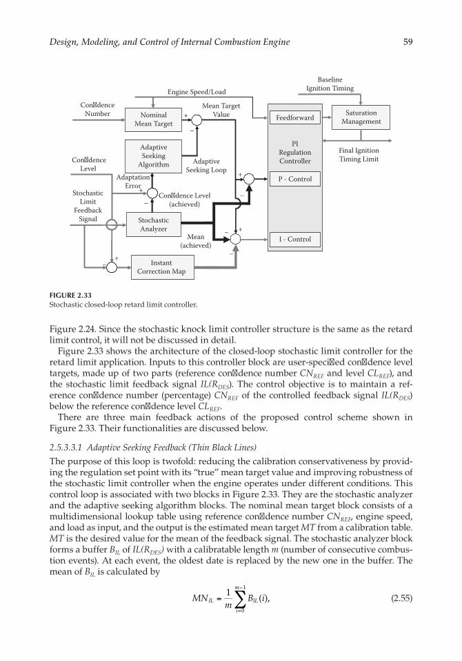
59Design, Modeling, and Control of Internal Combustion Engine
Figure 2.24. Since the stochastic knock limit controller structure is the same as the retard limit control, it will not be discussed in detail.
Figure 2.33 shows the architecture of the closed-loop stochastic limit controller for the retard limit application. Inputs to this controller block are user-specified confidence level targets, made up of two parts (reference confidence number CNREF and level CLREF), and the stochastic limit feedback signal IL(RDES). The control objective is to maintain a ref-erence confidence number (percentage) CNREF of the controlled feedback signal IL(RDES) below the reference confidence level CLREF.
There are three main feedback actions of the proposed control scheme shown in Figure 2.33. Their functionalities are discussed below.
2.5.3.3.1 Adaptive Seeking Feedback (Thin Black Lines)
The purpose of this loop is twofold: reducing the calibration conservativeness by provid-ing the regulation set point with its “true” mean target value and improving robustness of the stochastic limit controller when the engine operates under different conditions. This control loop is associated with two blocks in Figure 2.33. They are the stochastic analyzer and the adaptive seeking algorithm blocks. The nominal mean target block consists of a multidimensional lookup table using reference confidence number CNREF, engine speed, and load as input, and the output is the estimated mean target MT from a calibration table. MT is the desired value for the mean of the feedback signal. The stochastic analyzer block forms a buffer BIL of IL(RDES) with a calibratable length m (number of consecutive combus-tion events). At each event, the oldest date is replaced by the new one in the buffer. The mean of BIL is calculated by
1
( ),0
1
MNm
B iIL IL
i
m
∑==
−
(2.55)
Mean(achieved)
Engine Speed/Load
SaturationManagement
BaselineIgnition Timing
I - Control
P - Control
PIRegulationController
Final IgnitionTiming Limit
StochasticAnalyzer
AdaptationError
+
–
+
+
–Instant
Correction Map
+
–
–
+–
–
AdaptiveSeeking Loop
Feedforward
Con�denceNumber
Mean TargetValueNominal
Mean Target
Con�denceLevel
AdaptiveSeeking
Algorithm
Con�dence Level(achieved)
StochasticLimit
FeedbackSignal
FIGURE 2.33Stochastic closed-loop retard limit controller.

60 Design and Control of Automotive Propulsion Systems
and actual confidence number CNACT can be calculated by
CN
B i I i
B i
ACT
IL B
i
m
IL
i
m
∑
∑=
⋅
×=
−
=
−
( ) ( )
( )
100%,0
1
0
1 (2.56)
where IB (i) = 1 if BIL (i) ≤ CLREF; otherwise, IB (i) = 0.The actual confidence level CLACT of a given confidence number CNREF is another
parameter of interest. Define BIL as a reordered vector of BIL with its elements arranged in an increased order. Then the actual confidence level can be defined as follows:
CL B kACT IL= ( ). (2.57)
where k is the closest integer of m ⋅ CLREF . The adaptive seeking algorithm utilizes adap-tation error (CLREF − CLACT) as input, and the output is mean target correction (MTC) obtained by integrating the adaptation error with a calibration gain. This control loop is used to reduce the conservativeness of the mean target MT for the regulation controller discussed next.
2.5.3.3.2 Regulation Stochastic Feedback (Thick Black Line)
The regulation loop is used to regulate the mean value of the stochastic limit feedback signal to a mean target value. The regulation controller is structured as a PI controller and a feedforward term based on engine operating conditions. The error input to the PI controller is
errPI = MT − MTC − MNIL. (2.58)
Despite the variability of the stochastic retard limit feedback signal IL(RDES), its mean value is a well-behaved signal for regulation purposes. The regulation controller is tuned to provide the desired settling time and steady-state accuracy for the response.
2.5.3.3.3 Instant Correction Feedback (Thick Gray Line)
This block calculates an instant correction signal to be fed into the integration portion of the PI controller. The instant correction is generated by a lookup table using the error signal CLREF − IL(RDES) as input. When the error is greater than zero, the output is zero, and when the error is less than zero, the output is positive and increases as the input becomes more negative. Feeding the instant correction to the integral term is equivalent to the role of counter-up/down logic. Instant correction refers to a spark retard action at the next com-bustion event; the gain determines how much spark retard is generated for the excessive knock intensity value over the threshold.
For knock limit control, the same controller structure was used. The stochastic limit feedback signal IL(RDES) is replaced by calculated IKNK, and the details can be found in [76].
The interaction of the stochastic limit controllers with the MBT controller is managed by the spark timing limit management block in Figure 2.24. This interaction may be illus-trated using the retard limit control as an example. If the baseline spark timing is more advanced than the current retard limit, then the baseline spark is used as it is. In that
61Design, Modeling, and Control of Internal Combustion Engine
case, the retard limit controller pushes the limit in the maximum retard direction by itself. This is due to the fact that the limit controller integrator has a negative input and keeps integrating until the maximum retard allowed is reached (an antiwindup scheme is used). If the baseline spark controller pushes the spark timing to a level at which the feedback signals generate corrections, then the retard spark limit moves from its maximum retard spark limit to a less retarded level as a variable saturation limit on the baseline spark. On the other hand, if the baseline spark continues pushing the spark in the retard direction even when the baseline spark is saturated, the seeking and instant correction actions of the retard controller will adjust the retard limit online.
2.5.4 Experimental Study Results
The experimental study of the proposed spark timing control strategy consists of three subsections. These subsections present the experimental results for closed-loop MBT timing and advanced and retard limit controllers. At the end of this section the results of an integrated ignition control system that combines the MBT timing controller with both advanced and retard limit controllers are shown.
The proposed control system was validated in an engine dynamometer. The engine was controlled by the engine dynamometer except for engine spark timing. The engine dyna-mometer controlled the engine throttle position, EGR rate, and fuel injection. It also con-trolled the engine speed and load. A rapid prototype controller was used for prototyping both open-loop and closed-loop spark timing control. Laboratory-grade pressure sensors were installed in every cylinder for comparing with in-cylinder ionization signals.
The digital waveform capture card inside the rapid prototype controller generates the interrupt based upon the crankshaft encoder pulses that trigger the data sampling process. A calculated crank angle also generates a software interrupt to initiate the combustion event-based closed-loop ignition control calculation. The spark timing is calculated during exhaust stroke of the corresponding cylinder to make the spark control commands avail-able before the intake stroke. The closed-loop control algorithms, shown in Figure 2.33, run every combustion event.
2.5.4.1 Closed-Loop MBT Timing Control
Before the results of closed-loop MBT timing control are discussed, results demonstrating the validity of the composite MBT timing criterion are presented on an example operating point. Figure 2.34 shows the estimated MBT timing criterion CMBT when the engine was running at 1500 rpm with 7.0 bar BMEP load, and the ignition timing is at its MBT timing (21° before TDC). The data shown in Figure 2.34 are 100 cycles of data for cylinder 3 only. It can be observed that the MBT criterion confirms that the engine is operated close to its MBT timing since the average of the calculated CMBT is close to zero. This ionization MBT timing detection algorithm was validated over the entire engine operational map using offline test data.
Figure 2.35 shows the relationship between estimated ionization MBT criterion CMBT and in-cylinder pressure MBT criteria MAMFB, 50% MFB, and PCPL, where MAMFB is the maximum acceleration point of MFB calculated from in-cylinder pressure signal [68], which is defined as the peak location of the second derivative of MFB. The data shown in Figure 2.35 are a result of spark timing sweep when the engine was operated at 1500 rpm with 7.0 bar BMEP load. The spark timing varies from 13° to 25° before TDC. The top graph of Figure 2.35 shows the MBT timing criteria for cylinder 3, and the bottom one shows
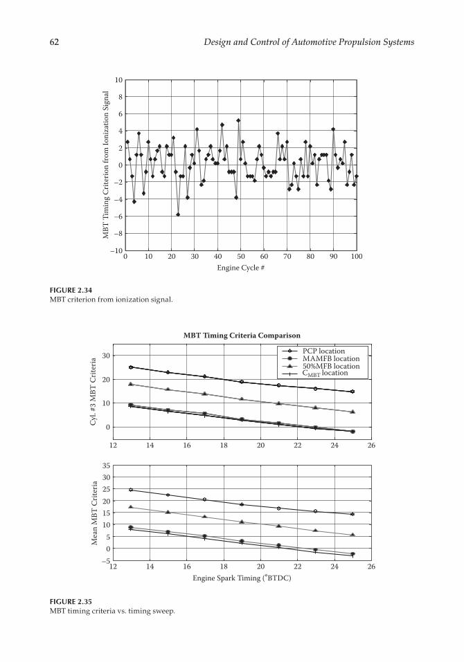
62 Design and Control of Automotive Propulsion Systems
0 10 20 30 40 50 60 70 80 90 100–10
–8
–6
–4
–2
0
2
4
6
8
10
Engine Cycle #
MBT
Tim
ing
Crite
rion
from
Ioni
zatio
n Si
gnal
FIGURE 2.34MBT criterion from ionization signal.
MBT Timing Criteria Comparison
12 14 16 18 20 22 24 26
0
10
20
30
Cyl.
#3 M
BT C
riter
ia
PCP locationMAMFB location50%MFB location
12 14 16 18 20 22 24 26–505
101520253035
Engine Spark Timing (°BTDC)
Mea
n M
BT C
riter
ia
CMBT location
FIGURE 2.35MBT timing criteria vs. timing sweep.
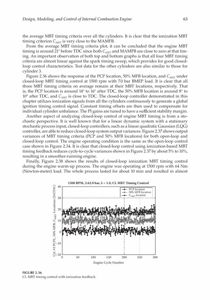
63Design, Modeling, and Control of Internal Combustion Engine
the average MBT timing criteria over all the cylinders. It is clear that the ionization MBT timing criterion CMBT is very close to the MAMFB.
From the average MBT timing criteria plot, it can be concluded that the engine MBT timing is around 21° before TDC since both CMBT and MAMFB are close to zero at that tim-ing. An important observation of both top and bottom graphs is that all four MBT timing criteria are almost linear against the spark timing sweep, which provides for good closed-loop control characteristics. Test data for the other cylinders are also similar to those for cylinder 3.
Figure 2.36 shows the response of the PCP location, 50% MFB location, and CMBT under closed-loop MBT timing control at 1500 rpm with 7.0 bar BMEP load. It is clear that all three MBT timing criteria on average remain at their MBT locations, respectively. That is, the PCP location is around 14° to 16° after TDC, the 50% MFB location is around 8° to 10° after TDC, and CMBT is close to TDC. The closed-loop controller demonstrated in this chapter utilizes ionization signals from all the cylinders continuously to generate a global ignition timing control signal. Constant timing offsets are then used to compensate for individual cylinder unbalance. The PI gains are tuned to have a sufficient stability margin.
Another aspect of analyzing closed-loop control of engine MBT timing is from a sto-chastic perspective. It is well known that for a linear dynamic system with a stationary stochastic process input, closed-loop controllers, such as a linear quadratic Gaussian (LQG) controller, are able to reduce closed-loop system output variances. Figure 2.37 shows output variances of MBT timing criteria (PCP and 50% MFB locations) for both open-loop and closed-loop control. The engine operating condition is the same as the open-loop control case shown in Figure 2.34. It is clear that closed-loop control using ionization-based MBT timing feedback reduces cycle-to-cycle variances shown in Figure 2.37 by about 5% to 10%, resulting in a smoother-running engine.
Finally, Figure 2.38 shows the results of closed-loop ionization MBT timing control during the engine warm-up process. The engine was operating at 1500 rpm with 64 Nm (Newton-meter) load. The whole process lasted for about 10 min and resulted in almost
1500 RPM, 2.62.0 bar, λ = 1.0, CL MBT Timing Control
PCP location50% MFB locationCMBT location
Engine Cycle Number150100500
–20
–10
0
10
Cyl.
#3 P
CPL
, 50%
MFB
, CM
BT L
ocat
ions
(DAT
DC
)
20
30
40
200 250 300
FIGURE 2.36CL MBT timing control with ionization feedback.
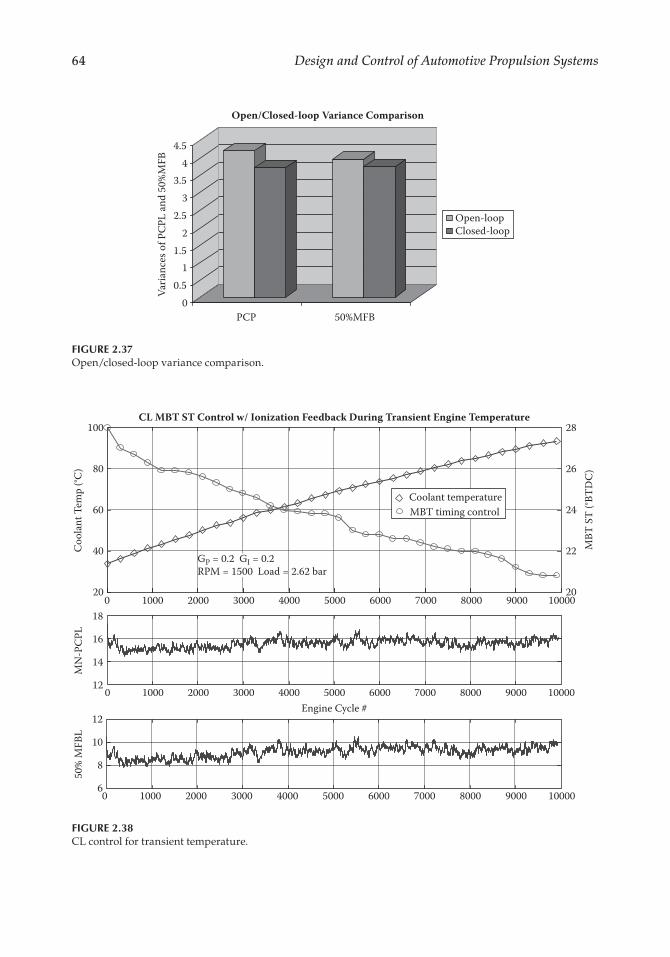
64 Design and Control of Automotive Propulsion Systems
00.5
11.5
22.5
33.5
44.5
Varia
nces
of P
CPL
and
50%M
FB
PCP 50%MFB
Open/Closed-loop Variance Comparison
Open-loopClosed-loop
FIGURE 2.37Open/closed-loop variance comparison.
0 1000 2000 3000 4000 5000 6000 7000 8000 9000 1000020
40
60
80
100
Cool
ant T
emp
(°C)
20
22
24
26
28
MBT
ST
(°BTD
C)
CL MBT ST Control w/ Ionization Feedback During Transient Engine Temperature
GP = 0.2 GI = 0.2RPM = 1500 Load = 2.62 bar
0 1000 2000 3000 4000 5000 6000 7000 8000 9000 100006
8
10
12
50%
MFB
L
0 1000 2000 3000 4000 5000 6000 7000 8000 9000 1000012
14
16
18
MN
-PC
PL
Engine Cycle #
Coolant temperatureMBT timing control
FIGURE 2.38CL control for transient temperature.
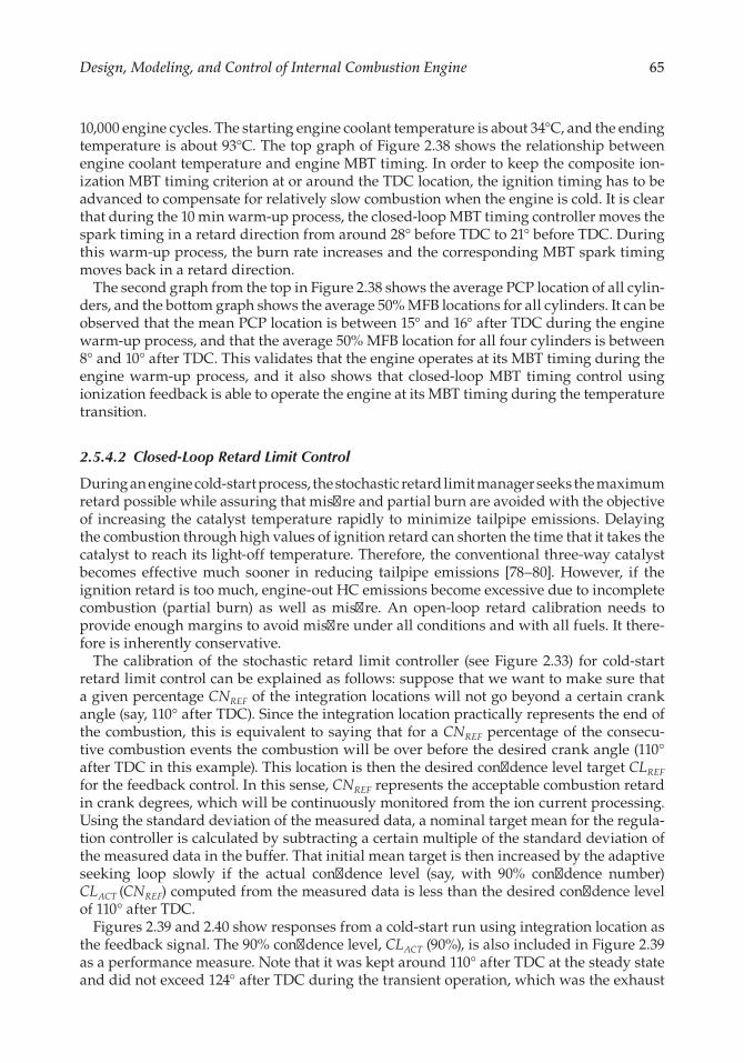
65Design, Modeling, and Control of Internal Combustion Engine
10,000 engine cycles. The starting engine coolant temperature is about 34°C, and the ending temperature is about 93°C. The top graph of Figure 2.38 shows the relationship between engine coolant temperature and engine MBT timing. In order to keep the composite ion-ization MBT timing criterion at or around the TDC location, the ignition timing has to be advanced to compensate for relatively slow combustion when the engine is cold. It is clear that during the 10 min warm-up process, the closed-loop MBT timing controller moves the spark timing in a retard direction from around 28° before TDC to 21° before TDC. During this warm-up process, the burn rate increases and the corresponding MBT spark timing moves back in a retard direction.
The second graph from the top in Figure 2.38 shows the average PCP location of all cylin-ders, and the bottom graph shows the average 50% MFB locations for all cylinders. It can be observed that the mean PCP location is between 15° and 16° after TDC during the engine warm-up process, and that the average 50% MFB location for all four cylinders is between 8° and 10° after TDC. This validates that the engine operates at its MBT timing during the engine warm-up process, and it also shows that closed-loop MBT timing control using ionization feedback is able to operate the engine at its MBT timing during the temperature transition.
2.5.4.2 Closed-Loop Retard Limit Control
During an engine cold-start process, the stochastic retard limit manager seeks the maximum retard possible while assuring that misfire and partial burn are avoided with the objective of increasing the catalyst temperature rapidly to minimize tailpipe emissions. Delaying the combustion through high values of ignition retard can shorten the time that it takes the catalyst to reach its light-off temperature. Therefore, the conventional three-way catalyst becomes effective much sooner in reducing tailpipe emissions [78–80]. However, if the ignition retard is too much, engine-out HC emissions become excessive due to incomplete combustion (partial burn) as well as misfire. An open-loop retard calibration needs to provide enough margins to avoid misfire under all conditions and with all fuels. It there-fore is inherently conservative.
The calibration of the stochastic retard limit controller (see Figure 2.33) for cold-start retard limit control can be explained as follows: suppose that we want to make sure that a given percentage CNREF of the integration locations will not go beyond a certain crank angle (say, 110° after TDC). Since the integration location practically represents the end of the combustion, this is equivalent to saying that for a CNREF percentage of the consecu-tive combustion events the combustion will be over before the desired crank angle (110° after TDC in this example). This location is then the desired confidence level target CLREF for the feedback control. In this sense, CNREF represents the acceptable combustion retard in crank degrees, which will be continuously monitored from the ion current processing. Using the standard deviation of the measured data, a nominal target mean for the regula-tion controller is calculated by subtracting a certain multiple of the standard deviation of the measured data in the buffer. That initial mean target is then increased by the adaptive seeking loop slowly if the actual confidence level (say, with 90% confidence number) CLACT (CNREF) computed from the measured data is less than the desired confidence level of 110° after TDC.
Figures 2.39 and 2.40 show responses from a cold-start run using integration location as the feedback signal. The 90% confidence level, CLACT (90%), is also included in Figure 2.39 as a performance measure. Note that it was kept around 110° after TDC at the steady state and did not exceed 124° after TDC during the transient operation, which was the exhaust
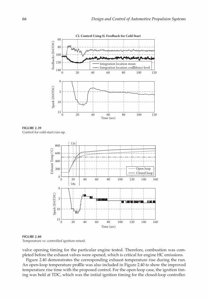
66 Design and Control of Automotive Propulsion Systems
valve opening timing for the particular engine tested. Therefore, combustion was com-pleted before the exhaust valves were opened, which is critical for engine HC emissions.
Figure 2.40 demonstrates the corresponding exhaust temperature rise during the run. An open-loop temperature profile was also included in Figure 2.40 to show the improved temperature rise time with the proposed control. For the open-loop case, the ignition tim-ing was held at TDC, which was the initial ignition timing for the closed-loop controller.
CL Control Using IL Feedback for Cold Start60
80
100
120
140
0
5
10
150 20 40 60 80 100 120
0 20 40 60
Integration location mean
Feed
back
s (D
ATD
C)
Spar
k (D
ATD
C)
Integration location con�dence level
Time (sec)
80 100 120
FIGURE 2.39Control for cold-start run-up.
12s
18s
Open loopClosed loop
800
600
400
200
00 20 40 60 80 100 120 140 160
015
10
5
0
20 40 60 80Time (sec)
Spar
k (D
ATD
C)
Exha
ust T
emp
(°C)
100 120 140 160
FIGURE 2.40Temperature vs. controlled ignition retard.
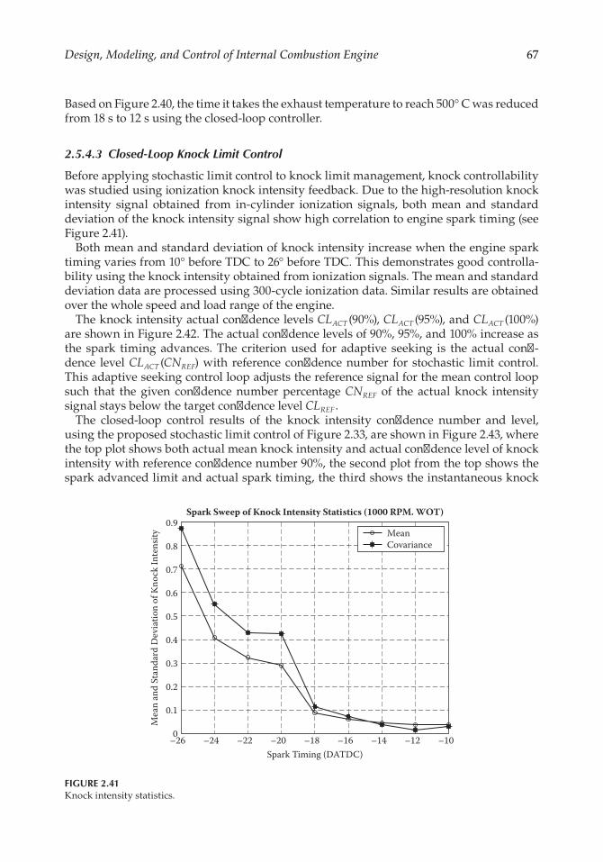
67Design, Modeling, and Control of Internal Combustion Engine
Based on Figure 2.40, the time it takes the exhaust temperature to reach 500° C was reduced from 18 s to 12 s using the closed-loop controller.
2.5.4.3 Closed-Loop Knock Limit Control
Before applying stochastic limit control to knock limit management, knock controllability was studied using ionization knock intensity feedback. Due to the high-resolution knock intensity signal obtained from in-cylinder ionization signals, both mean and standard deviation of the knock intensity signal show high correlation to engine spark timing (see Figure 2.41).
Both mean and standard deviation of knock intensity increase when the engine spark timing varies from 10° before TDC to 26° before TDC. This demonstrates good controlla-bility using the knock intensity obtained from ionization signals. The mean and standard deviation data are processed using 300-cycle ionization data. Similar results are obtained over the whole speed and load range of the engine.
The knock intensity actual confidence levels CLACT (90%), CLACT (95%), and CLACT (100%)are shown in Figure 2.42. The actual confidence levels of 90%, 95%, and 100% increase as the spark timing advances. The criterion used for adaptive seeking is the actual confi-dence level CLACT (CNREF) with reference confidence number for stochastic limit control. This adaptive seeking control loop adjusts the reference signal for the mean control loop such that the given confidence number percentage CNREF of the actual knock intensity signal stays below the target confidence level CLREF .
The closed-loop control results of the knock intensity confidence number and level, using the proposed stochastic limit control of Figure 2.33, are shown in Figure 2.43, where the top plot shows both actual mean knock intensity and actual confidence level of knock intensity with reference confidence number 90%, the second plot from the top shows the spark advanced limit and actual spark timing, the third shows the instantaneous knock
Mean
Spark Sweep of Knock Intensity Statistics (1000 RPM. WOT)0.9
0.8
0.7
0.6
0.5
0.4
0.3
0.2
0.1
0–26 –24 –22 –20 –18Spark Timing (DATDC)
–16 –14 –12 –10
Mea
n an
d St
anda
rd D
evia
tion
of K
nock
Inte
nsity
Covariance
FIGURE 2.41Knock intensity statistics.

68 Design and Control of Automotive Propulsion Systems
98%95%
Actual Con�dence Level with Di�erent Con�denceNumbers (1000 RPM, WOT)
4.5
4
3.5
3
2.5
2
1.5
1
0.5
0–26 –24 –22 –20 –18Spark Timing (DATDC)
–16 –14 –12 –10
Actu
al C
on�d
ence
Lev
el o
f Kno
ck In
tens
ity (V
) 100%
FIGURE 2.42Knock intensity actual confidence levels.
Mean KICon�dence KI level
Advance limit
120100806040CL Knock Control Enabled
Adaptive Seeking Enabled
20
12010080604020
0
0 100806040200
120100806040200
1201008060Time (sec)
402000
10
20
30
1.5
1
0.5
–1.5
–2.0
–1.0
0
0
2
4
Inst
ant K
I (V
)%
Ove
r 0.1
VSp
ark
(DAT
DC
)St
ats o
f KI (
V)
Applied spark
Con�dence LevelTarget (0.1 V)
FIGURE 2.43CL knock limit control.
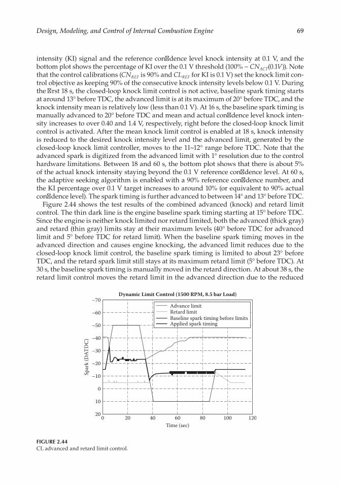
69Design, Modeling, and Control of Internal Combustion Engine
intensity (KI) signal and the reference confidence level knock intensity at 0.1 V, and the bottom plot shows the percentage of KI over the 0.1 V threshold (100% − CNACT(0.1V)). Note that the control calibrations (CNREF is 90% and CLREF for KI is 0.1 V) set the knock limit con-trol objective as keeping 90% of the consecutive knock intensity levels below 0.1 V. During the first 18 s, the closed-loop knock limit control is not active, baseline spark timing starts at around 13° before TDC, the advanced limit is at its maximum of 20° before TDC, and the knock intensity mean is relatively low (less than 0.1 V). At 16 s, the baseline spark timing is manually advanced to 20° before TDC and mean and actual confidence level knock inten-sity increases to over 0.40 and 1.4 V, respectively, right before the closed-loop knock limit control is activated. After the mean knock limit control is enabled at 18 s, knock intensity is reduced to the desired knock intensity level and the advanced limit, generated by the closed-loop knock limit controller, moves to the 11~12° range before TDC. Note that the advanced spark is digitized from the advanced limit with 1° resolution due to the control hardware limitations. Between 18 and 60 s, the bottom plot shows that there is about 5% of the actual knock intensity staying beyond the 0.1 V reference confidence level. At 60 s, the adaptive seeking algorithm is enabled with a 90% reference confidence number, and the KI percentage over 0.1 V target increases to around 10% (or equivalent to 90% actual confidence level). The spark timing is further advanced to between 14° and 13° before TDC.
Figure 2.44 shows the test results of the combined advanced (knock) and retard limit control. The thin dark line is the engine baseline spark timing starting at 15° before TDC. Since the engine is neither knock limited nor retard limited, both the advanced (thick gray) and retard (thin gray) limits stay at their maximum levels (40° before TDC for advanced limit and 5° before TDC for retard limit). When the baseline spark timing moves in the advanced direction and causes engine knocking, the advanced limit reduces due to the closed-loop knock limit control, the baseline spark timing is limited to about 23° before TDC, and the retard spark limit still stays at its maximum retard limit (5° before TDC). At 30 s, the baseline spark timing is manually moved in the retard direction. At about 38 s, the retard limit control moves the retard limit in the advanced direction due to the reduced
Dynamic Limit Control (1500 RPM, 8.5 bar Load)
60 80 100 120020
10
0
–10
–20
Spar
k (D
ATD
C)
–30
–40
–50
–60
–70
20 40Time (sec)
Advance limitRetard limitBaseline spark timing before limitsApplied spark timing
FIGURE 2.44CL advanced and retard limit control.
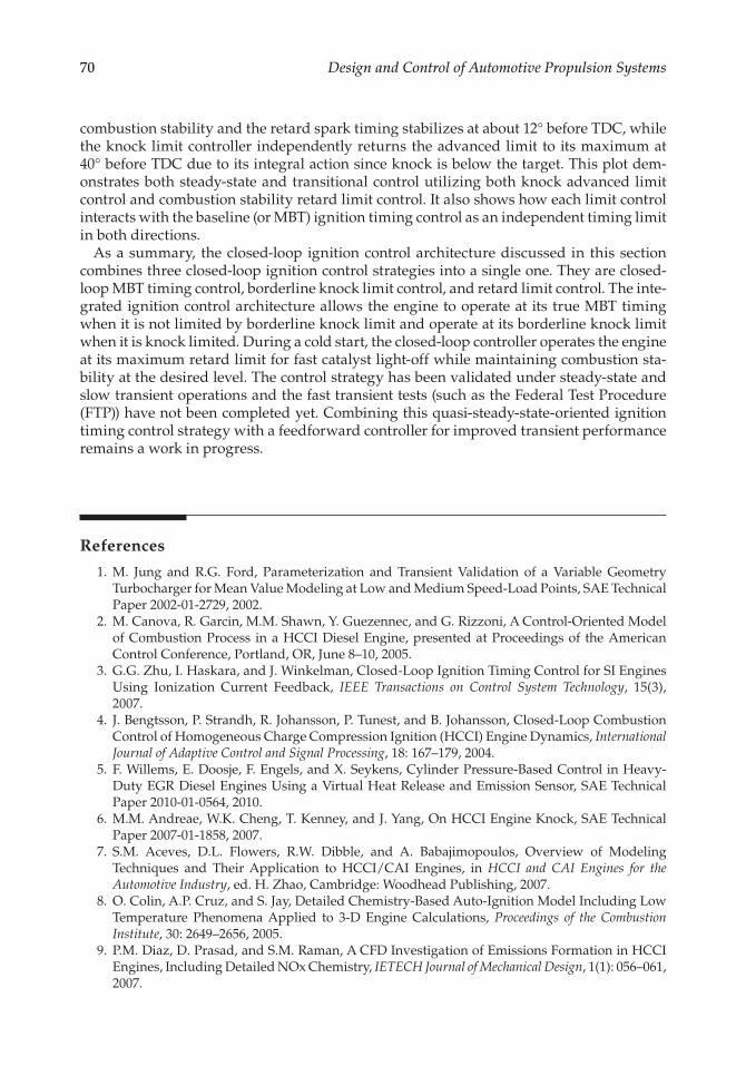
70 Design and Control of Automotive Propulsion Systems
combustion stability and the retard spark timing stabilizes at about 12° before TDC, while the knock limit controller independently returns the advanced limit to its maximum at 40° before TDC due to its integral action since knock is below the target. This plot dem-onstrates both steady-state and transitional control utilizing both knock advanced limit control and combustion stability retard limit control. It also shows how each limit control interacts with the baseline (or MBT) ignition timing control as an independent timing limit in both directions.
As a summary, the closed-loop ignition control architecture discussed in this section combines three closed-loop ignition control strategies into a single one. They are closed-loop MBT timing control, borderline knock limit control, and retard limit control. The inte-grated ignition control architecture allows the engine to operate at its true MBT timing when it is not limited by borderline knock limit and operate at its borderline knock limit when it is knock limited. During a cold start, the closed-loop controller operates the engine at its maximum retard limit for fast catalyst light-off while maintaining combustion sta-bility at the desired level. The control strategy has been validated under steady-state and slow transient operations and the fast transient tests (such as the Federal Test Procedure (FTP)) have not been completed yet. Combining this quasi-steady-state-oriented ignition timing control strategy with a feedforward controller for improved transient performance remains a work in progress.
References
1. M. Jung and R.G. Ford, Parameterization and Transient Validation of a Variable Geometry Turbocharger for Mean Value Modeling at Low and Medium Speed-Load Points, SAE Technical Paper 2002-01-2729, 2002.
2. M. Canova, R. Garcin, M.M. Shawn, Y. Guezennec, and G. Rizzoni, A Control-Oriented Model of Combustion Process in a HCCI Diesel Engine, presented at Proceedings of the American Control Conference, Portland, OR, June 8–10, 2005.
3. G.G. Zhu, I. Haskara, and J. Winkelman, Closed-Loop Ignition Timing Control for SI Engines Using Ionization Current Feedback, IEEE Transactions on Control System Technology, 15(3), 2007.
4. J. Bengtsson, P. Strandh, R. Johansson, P. Tunest, and B. Johansson, Closed-Loop Combustion Control of Homogeneous Charge Compression Ignition (HCCI) Engine Dynamics, International Journal of Adaptive Control and Signal Processing, 18: 167–179, 2004.
5. F. Willems, E. Doosje, F. Engels, and X. Seykens, Cylinder Pressure-Based Control in Heavy-Duty EGR Diesel Engines Using a Virtual Heat Release and Emission Sensor, SAE Technical Paper 2010-01-0564, 2010.
6. M.M. Andreae, W.K. Cheng, T. Kenney, and J. Yang, On HCCI Engine Knock, SAE Technical Paper 2007-01-1858, 2007.
7. S.M. Aceves, D.L. Flowers, R.W. Dibble, and A. Babajimopoulos, Overview of Modeling Techniques and Their Application to HCCI/CAI Engines, in HCCI and CAI Engines for the Automotive Industry, ed. H. Zhao, Cambridge: Woodhead Publishing, 2007.
8. O. Colin, A.P. Cruz, and S. Jay, Detailed Chemistry-Based Auto-Ignition Model Including Low Temperature Phenomena Applied to 3-D Engine Calculations, Proceedings of the Combustion Institute, 30: 2649–2656, 2005.
9. P.M. Diaz, D. Prasad, and S.M. Raman, A CFD Investigation of Emissions Formation in HCCI Engines, Including Detailed NOx Chemistry, IETECH Journal of Mechanical Design, 1(1): 056–061, 2007.
71Design, Modeling, and Control of Internal Combustion Engine
10. Gamma Technology, Engine Performance Application Manual, GT-Suite version 7.0, September 2009. Available at http://www.gtisoft.com/.
11. L. Guzzella and C.H. Onder, Introduction to Modeling and Control of Internal Combustion Engine Systems, Berlin: Springer, 2004.
12. S. Saulnier and S. Guiliain, Computational Study of Diesel Engine Downsizing Using Two-Stage Turbocharging, SAE Technical Paper 2004-01-0929, 2004.
13. A.Y. Karnik, J.H. Buckland, and J.S. Freudenberg, Electronic Throttle and Wastegate Control for Turbocharged Gasoline Engines, in Proceedings of the American Control Conference, Portland, OR, 2005, pp. 4434–4439.
14. K.L. Hoag and R.J. Primus, Fundamentals of Diesel Engine Performance, Cummins Engine Company, Columbus, IN, 1992.
15. X. Yang and G. Zhu, A Mixed Mean-Value and Event-Based Model of a Dual-Stage Turbocharged SI Engine for Hardware-in-the-Loop Simulation, presented at Proceedings of the American Control Conference, Baltimore, MD, June 2010.
16. X. Yang and G. Zhu, A Control Oriented Hybrid Combustion Model of an HCCI Capable SI Engine, Journal of Automobile Engineering, 226(10): 1380–1395, 2012.
17. S. Zhang, G. Zhu, and Z. Sun, A Control-Oriented Charge Mixing and Two-Zone HCCI Combustion Model, IEEE Transactions on Vehicular Technology, 63(3): 1079–1090, 2014.
18. M. Locatelli, C.H. Onder, and H.P. Geering, An Easily Tunable Wall-Wetting Model for PFI Engines, SAE Technical Paper 2004-01-1461, 2004.
19. J.B. Heywood, Internal Combustion Engine Fundamentals, McGraw-Hill, New York City, NY, 1988. 20. A. Lefebvre and S. Guilain, Modeling and Measurement of the Transient Response of a
Turbocharged SI Engine, SAE Technical Paper 2005-01-0691, 2005. 21. G.M. Shaver, M.J. Roelle, and J.C. Gerdes, Modeling Cycle-to-Cycle Dynamics and Mode Transition
in HCCI Engines with Variable Valve Actuation, Control Engineering Practice, 14: 213–222, 2006. 22. J. Chang and O. Guralp, New Heat Transfer Correlation for an HCCI Engine Derived from
Measurements of Instantaneous Surface Heat Flux, SAE Technical Paper 2004-01-2996, 2004. 23. K. Inoue, K. Nagakiro, Y. Ajiki, and N. Kishi, A High Power Wide Torque Range Efficient
Engine with a Newly Developed Variable Valve Lift and Timing Mechanism, SAE Technical Paper 890675, 1989.
24. Y. Moriya, A. Watanabe, H. Uda, H. Kawamura, M. Yoshioka, and M. Adachi, A Newly Developed Intelligent Variable Valve Timing System—Continuously Controlled Cam Phasing as Applied to a New 3 Liter Inline 6 Engine, SAE Technical Paper 960579, 1996.
25. K.H. Oehling, R. Teichmann, and H. Unger, Requirements and Potentials of Future Valve Train Concepts, SAE Technical Paper 964211, 1996.
26. R. Flierl and M. Kluting, The Third Generation of Valvetrains—New Fully Variable Valvetrain for Throttle Free Load Control, SAE Technical Paper 2000-01-1227, 2000.
27. M. Theobald, B. Lequesne, and R. Henry, Control of Engine Load via Electromagnetic Valve Actuators, SAE Technical Paper 940816, 1994.
28. P. Kreuter, P. Heuser, and M. Schebitz, Strategies to Improve SI-Engine Performance by Means of Variable Intake Lift, Timing and Duration, SAE Technical Paper 920449, 1992.
29. M. Schecter and M. Levin, Camless Engine, SAE Technical Paper 960581, 1996. 30. C. Turner, G. Babbitt, C. Balton, M. Raimao, and D. Giordano, Design and Control of a Two-
Stage Electro-Hydraulic Valve Actuation System, SAE Technical Paper 2004-01-1265, 2004. 31. J. Allen and D. Law, Production Electro-Hydraulic Variable Valve-Train for a New Generation
of I.C. Engines, SAE Technical Paper 2002-01-1109, 2002. 32. D. Denger and K. Mischker, The Electro-Hydraulic Valvetrain System EHVS—System and
Potential, SAE Technical Paper 2005-01-0774, 2005. 33. J. Watson and R. Wakeman, Simulation of a Pneumatic Valve Actuation System for Internal
Combustion Engine, SAE Technical Paper 2005-01-0771, 2005. 34. J. Ma, H. Schock, U. Carlson, A. Hoglund, and M. Hedman, Analysis and Modeling of an
Electronically Controlled Pneumatic Hydraulic Valve for an Automotive Engine, SAE Technical Paper 2006-01-0042, 2006.

72 Design and Control of Automotive Propulsion Systems
35. R.M. Richman and W.C. Reynolds, A Computer-Controlled Poppet-Valve Actuation System for Application on Research Engines, SAE Technical Paper 840340, 1984.
36. J. Turner, M. Bassett, R. Pearson, G. Pitcher, and K. Douglas, New Operating Strategies Afforded by Fully Variable Valve Trains, SAE Technical Paper 2004-01-1386, 2004.
37. Z. Sun and D. Cleary, Dynamics and Control of an Electro-Hydraulic Fully Flexible Valve Actuation System, in Proceedings of the American Control Conference, Denver, CO, 2003, pp. 3119–3124.
38. Z. Sun and T. Kuo, Electro-Hydraulic Fully Flexible Valve Actuation System for Advanced Combustion Development, in Proceedings of the FISITA World Congress, Yokohama, Japan, F2006P287, 2006.
39. Z. Sun and H. Xin, Development and Control of Electro-Hydraulic Fully Flexible Valve Actuation System for Diesel Combustion Research, SAE Technical Paper 2007-01-4021, 2007.
40. Z. Sun, Engine Valve Actuation Assembly with Dual Automatic Regulation, U.S. Patent 6,959,673, 2005.
41. P. Gillella and Z. Sun, Design, Modeling, and Control of a Camless Valve Actuation System with Internal Feedback, IEEE/ASME Transactions on Mechatronics, 16(3): 527–539, 2011.
42. Z. Sun, Electrohydraulic Fully Flexible Valve Actuation System with Internal Feedback, Journal of Dynamic Systems, Measurement, and Control, 131: 024502, 2009.
43. M. Anderson, T.-C. Tsao, and M. Levin, Adaptive Lift Control for a Camless Electrohydraulic Valvetrain, SAE Technical Paper 981029, 1998.
44. K. Misovec, B. Johnson, G. Mansouri, O. Sturman, and S. Massey, Digital Valve Technology Applied to the Control of a Hydraulic Valve Actuator, SAE Technical Paper 1999-01-0825, 1999.
45. W. Hoffmann and A.G. Stefanopoulou, Iterative Learning Control of Electromechanical Camless Valve Actuator, in Proceedings of the American Control Conference, Arlington, VA, 2001, pp. 2860–2866.
46. C. Tai and T.-C. Tsao, Control of an Electromechanical Camless Valve Actuator, in Proceedings of the American Control Conference, Anchorage, AK, 2002, pp. 262–267.
47. Z. Sun and T.-W. Kuo, Transient Control of Electro-Hydraulic Fully Flexible Engine Valve Actuation System, IEEE Transactions on Control Systems Technology, 18: 613–621, 2010.
48. M. Tomizuka, T.-C. Tsao, and K.-K. Chew, Analysis and Synthesis of Discrete-Time Repetitive Controllers, Journal of Dynamic Systems, Measurement, and Control, 111: 353–358, 1989.
49. T.-C. Tsao and M. Tomizuka, Robust Adaptive and Repetitive Digital Tracking Control and Application to a Hydraulic Servo for Noncircular Machining, Journal of Dynamic Systems, Measurement, and Control, 116: 24–32, 1994.
50. D.H. Kim and T.-C. Tsao, A Linearized Electrohydraulic Servovalve Model for Valve Dynamics Sensitivity Analysis and Control System Design, Journal of Dynamic Systems, Measurement, and Control, 122: 179–187, 2000.
51. P. Gillella, X. Song, and Z. Sun, Time-Varying Internal Model-Based Control of a Camless Engine Valve Actuation System, IEEE Transactions on Control Systems Technology, 22(4): 1498–1510, 2014.
52. F.Q. Zhao, D.L. Harrington, and M.C. Lai, Automotive Direct-Injection Gasoline Engines, Society of Automotive Engineers Press, Warrendale, PA, 2002.
53. F.J. Hamady, J.P. Hahn, K.H. Hellman, and C.L. Gray Jr., High-Speed/High-Resolution Imaging of Fuel Sprays from Various Injector Nozzles for Direct Injection Engines, SAE Technical Paper 950289, 1994.
54. K. Kawajiri, T. Yonezawa, H. Ohuchi, M. Sumida, and H. Katashiba, Study of Interaction between Spray and Air Motion, and Spray Wall Impingement, SAE Technical Paper 2002-01-0836, 2002.
55. M. Jansons, S. Lin, and K.T. Rhee, High-Speed Imaging from Consecutive Cycles, SAE Technical Paper 2001-01-3486, 2001.

73Design, Modeling, and Control of Internal Combustion Engine
56. J.D. Smith and V. Sick, Crank-Angle Resolved Imaging of Fuel Distribution, Ignition and Combustion in a Direct-Injection Spark-Ignition Engine, SAE Technical Paper 2005-01-3753, 2005.
57. P. Wyszynski, R. Aboagye, R. Stone, and G. Kalghatgi, Combustion Imaging and Analysis in a Gasoline Direct Injection Engine, SAE Technical Paper 2004-01-0045, 2004.
58. D.L.S. Hung, W. Humphrey, L. Markle, D. Chmiel, C. Ospina, and F. Brado, A Novel Transient Drop Sizing Technique for Investigating the Role of Gasoline Injector Sprays in Fuel Mixture Preparation, SAE Technical Paper 2004-01-1349, 2004.
59. D.L.S. Hung, G. Zhu, J. Winkelman, T. Stuecken, H. Schock, and A. Fedewa, A High Speed Flow Visualization Study of Fuel Spray Pattern Effect on Mixture Formation in a Low Pressure Direct Injection Gasoline Engine, SAE Technical Paper 2007-01-1141, 2007.
60. D.L.S. Hung, D.L. Harrington, A.H. Gandhi, L.E. Markle, S.E. Parrish, J.S. Shakal, H. Sayar, S.D. Cummings, and J.L. Kramer, Gasoline Fuel Spray Measurement and Characterization—A New SAE J2715 Recommended Practice, SAE Technical Paper 2008-01-1068, 2008.
61. J.D. Powell, M. Hubbard, and R.R. Clappier, Ignition Timing Controls Method and Apparatus, U.S. Patent 4063538, 1977.
62. G.M. Rassweiler and L. Withrow, Motion Picture of Engine Flames Correlated with Pressure Cards, SAE Transactions, 42: 185–204, 1938.
63. M.C. Sellnau, F.A. Matekunas, P.A. Battiston, C.-F. Chang, and D.R. Lancaster, Cylinder-Pressure-Based Engine Control Using Pressure-Ratio-Management and Low-Cost Non-Intrusive Cylinder Pressure Sensor, SAE Technical Paper 2000-01-0932, 2000.
64. R.J. Hosey and J.D. Powell, Closed Loop, Knock Adaptive Spark Timing Control Based on Cylinder Pressure, Transactions of ASME, 101, 1979.
65. K. Sawamoto, Y. Kawamura, T. Kita, and K. Matsushita, Individual Cylinder Knock Control by Detecting Cylinder Pressure, SAE Technical Paper 871911, 1987.
66. Y. Kawamura, M. Shinshi, H. Sato, N. Takahshi, and M. Iriyama, MBT Control through Individual Cylinder Pressure Detection, SAE Technical Paper 881779, 1988.
67. R. Muller, M. Hart, G. Krotz, M. Eickhoff, A. Truscott, A. Nobel, C. Cavalloni, and M. Gnielka, Combustion Pressure Based Engine Management System, SAE Technical Paper 2000-01-0928, 2000.
68. G.G. Zhu, C.F. Daniels, and J. Winkelman, MBT Timing Detection and Its Closed-Loop Control Using In-Cylinder Pressure Signal, SAE Technical Paper 2003-01-3266, 2003.
69. L. Eriksson, Spark Advance Modeling and Control, PhD Dissertation, Linkoping University, 1999. 70. L. Eriksson and L. Nielsen, Closed Loop Ignition Control by Ionization Current Interpretation,
SAE Technical Paper 970854, 1997. 71. G. Zhu, I. Haskara, and J. Winkelman, Closed Loop Ignition Timing Control Using Ionization
Current Feedback, IEEE Transactions on Control System Technology, 15(3), 2007. 72. G.G. Zhu, C.F. Daniels, and J. Winkelman, MBT Timing Detection and Its Closed-Loop Control
Using In-Cylinder Ionization Signal, SAE Technical Paper 2004-01-2976, 2004. 73. C.F. Daniels, The Compression of Mass Fraction Burned Obtained from Cylinder Pressure
Signal and Spark Plug Ion Signal, SAE Technical Paper 980140, 1998. 74. R.J. Hosey and J.D. Powell, Closed Loop, Knock Adaptive Spark Timing Control Based on
Cylinder Pressure, Transactions of ASME, 101, 1979. 75. C.F. Daniels, G.G. Zhu, and J. Winkelman, Inaudible Knock and Partial Burn Detection Using
In-Cylinder Ionization Signal, SAE Technical Paper 2003-01-3149, 2003. 76. G.G. Zhu, I. Haskara, and J. Winkelman, Stochastic Limit Control and Its Application to Knock
Limit Control Using Ionization Feedback, SAE Technical Paper 2005-01-0018, 2005. 77. I. Haskara, G. Zhu, and J. Winkelman, IC Engine Retard Ignition Timing Limit Detection and
Control Using In-Cylinder Ionization Signal, SAE Technical Paper 2004-01-2977, 2004. 78. N.A. Henein and M.K. Tagomari, Cold-Start Hydrocarbon Emissions in Port-Injected Gasoline
Engines, Progress in Energy and Combustion Science, 25: 563–593, 1999. 79. J. Zhu and S.C. Chan, An Approach for Rapid Automotive Catalyst Light Off by High Values of
Ignition Retard, Journal of the Institute of Energy, 167–173, 1996.

74 Design and Control of Automotive Propulsion Systems
80. P. Tunestal, M. Wilcutts, A.T. Lee, and J.K. Hedrick, In-Cylinder Measurement for Engine Cold-Start Control, in Proceedings of the IEEE International Conference on Control Applications, Kohala Coast, HI, 1999, pp. 460–464.
81. J.D. Naber, J.R. Blough, D. Frankowski, M. Goble, and J.E. Szpytman, Analysis of Combustion Knock Metrics in Spark-Ignited Engines, SAE Technical Paper 2006-01-0400, 2006.
82. I. Haskara, G. Zhu, and J. Winkelman, Multivariable EGR/Spark Timing Control for IC Engines via Extremum Seeking, presented at Proceedings of the American Control Conference, Minneapolis, MN, 2006.

75
3Design, Modeling, and Control of Automotive Transmission Systems
3.1 Introduction to Various Transmission Systems
The basic function of a transmission is to transit power from the engine to the wheels of a vehicle. The fundamental reason why we need a transmission between the engine and the vehicle is again attributed back to the dynamic nature of vehicle operation. First, the vehicle requires both forward and reverse motion, while the engine only works in one direction. Therefore, a transmission that can reserve the output direction is needed. Second, the engine power, efficiency, and emissions are functions of the engine speed and load. To deliver the maximum power to the vehicle and maintain high fuel effi-ciency, different speed ratios are required between the engine and the vehicle. Third, it is desirable to reduce the driveline vibration caused by the engine firing pulse or the road disturbances. This is often referred to as drivability, which is a key attribute of the trans-mission system. Given the above reasons, the transmission is an indispensable part of the automotive propulsion system.
To realize the above functions, various transmissions have been designed, including the manual transmission (MT), automated manual transmission (AMT), dual-clutch transmis-sion (DCT), automatic transmission (AT), continuously variable transmission (CVT), etc. Both MT and AMT employ countershaft gears to realize different gear ratios. The DCT uses two sets of countershaft gears where the odd gears are on one set and the even gears on the other set. The countershaft gears are fairly flexible for designing the desired gear ratios and are extremely efficient for transmitting mechanical power, but they are not very compact given the fact that there are two parallel shafts and the gears are located along the axial direction of the shafts. The AT uses planetary gear sets to change the speed ratio. This is accomplished by connecting different nodes of the planetary gear sets (for details see Section 3.2). The planetary gears are fairly compact since they are concentric. But the gear ratio design is much more complicated than the MT. The CVT has several different variations: the belt system, the chain system, and the toroidal drive system. The belt and chain drive systems are suitable for low to medium torque applications, while the toroidal drive system has higher torque capacity. But overall the design of the CVT is more compli-cated than the stepped gear transmission.
Besides the different gear ratio mechanisms employed by different transmissions, the other key differentiator for the transmissions is the actuation and control methods for realizing the gear ratios in real time. The MT has the driver to control the gear ratio change by using a lever mechanism. A synchronization device is used to synchronize the speeds of the input shaft and the output shaft before a locking device is used to lock the shafts

76 Design and Control of Automotive Propulsion Systems
into the new gear ratio. The AT uses electrohydraulic clutches to realize the gear shift automatically. The gear shift schedule determines the timing for gear shift based on the vehicle speed and the throttle position. A hydraulic pump is connected directly to the engine that will produce the fluid power for actuating the clutches. Control valves are used to regulate the pressure and flow for appropriate gear shift. Frictional material is used for the clutch plate, and when compressed will engage the input and output shafts. The CVT also employs fluid power to change the speed ratio automatically in real time. But the control mechanism is more complicated due to the nature of continuous gear ratio change. The AMT uses either an electrical motor or a hydraulic actuator to change the gear ratio. The DCT has two clutches that can be engaged or disengaged in real time to real-ize the gear ratio change. One clutch is connected to the odd gears, and the other clutch is connected to the even gears. During gear shift, synchronization between the clutches is critical. For the rest of the chapter, we will mainly focus on the automatic transmission, while many results can also be applied to other types of transmissions.
3.2 Gear Ratio Realization for Automatic Transmission
3.2.1 Planetary Gear Set
Gear ratio change in an automatic transmission is realized by connecting different nodes of the planetary gear sets. As shown in Figure 3.1, a planetary gear set includes the sun gear, the ring gear, and the planet gear. The carrier connects the planet gears together. So the three nodes for a planetary gear set are sun, ring, and carrier.
To analyze the speed and torque of a planetary gear set, we use the lever diagram as shown in Figure 3.2, where SG represents the sun gear, C represents the carrier, and RG represents the ring gear. The length of the lever between SG and C is denoted as R, which
Ring Gear
Sun Gear
Planet
PlanetPlanet
Pinion
PlanetCarrier (PC)
Planet
Ring
Ring
Sun
FIGURE 3.1Diagram of a planetary gear set.

77Design, Modeling, and Control of Automotive Transmission Systems
corresponds to the number of teeth of the ring gear. Similarly, the length between RG and C is S, which corresponds to the number of teeth of the sun gear.
Let’s connect the carrier (node C) to the ground as shown in Figure 3.3. Now we are ready to apply the lever analogy to calculate the speed and torque at different nodes of the planetary gear set.
Based on Figure 3.3, we have
WW
SR
R
S= −
Based on Figure 3.4, we have
⋅ = ⋅
+ − == = + =
+T S T RT T T
T TRS
T T TS R
STR S
R S CR S C S R S0
,
With the above example, we introduce the following relationship for the planetary gear set:
Ts + TR − TC = 0
RG
C
SG
RG
C
SG
S
R
FIGURE 3.2Lever diagram.
S
R
C
RG
SG Ws
WR
FIGURE 3.3Speed calculation using lever diagram.
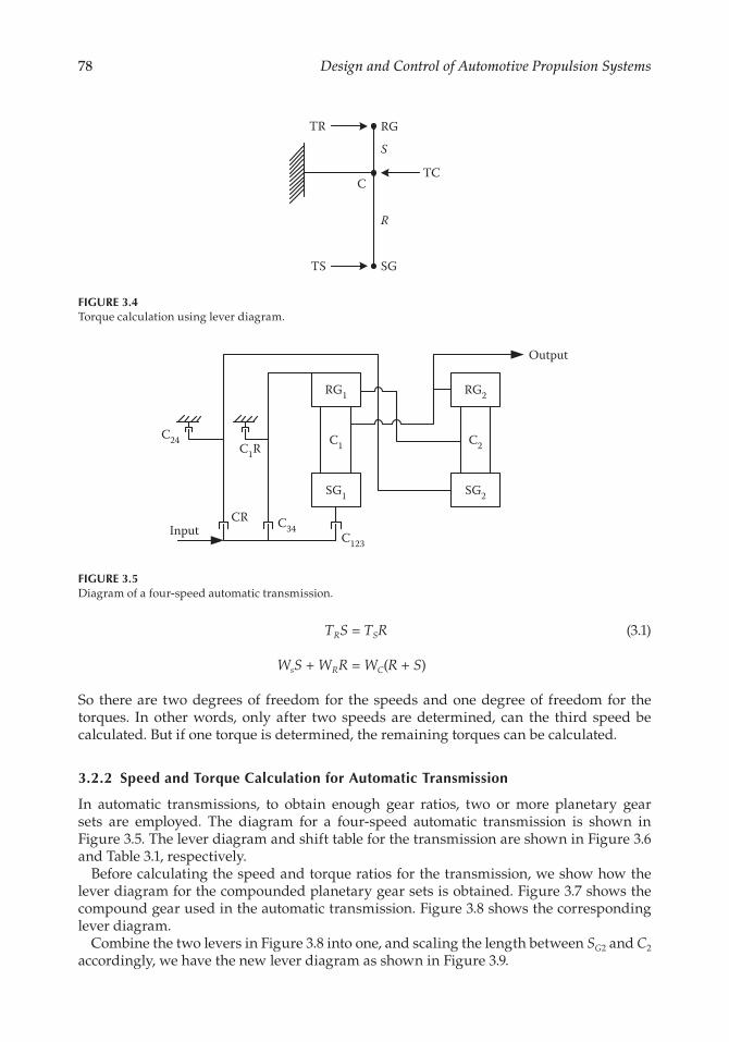
78 Design and Control of Automotive Propulsion Systems
TRS = TSR (3.1)
WsS + WRR = WC(R + S)
So there are two degrees of freedom for the speeds and one degree of freedom for the torques. In other words, only after two speeds are determined, can the third speed be calculated. But if one torque is determined, the remaining torques can be calculated.
3.2.2 Speed and Torque Calculation for Automatic Transmission
In automatic transmissions, to obtain enough gear ratios, two or more planetary gear sets are employed. The diagram for a four-speed automatic transmission is shown in Figure 3.5. The lever diagram and shift table for the transmission are shown in Figure 3.6 and Table 3.1, respectively.
Before calculating the speed and torque ratios for the transmission, we show how the lever diagram for the compounded planetary gear sets is obtained. Figure 3.7 shows the compound gear used in the automatic transmission. Figure 3.8 shows the corresponding lever diagram.
Combine the two levers in Figure 3.8 into one, and scaling the length between SG2 and C2 accordingly, we have the new lever diagram as shown in Figure 3.9.
RG1
SG1
C1
RG2
SG2
C2C24
CR C34C123
Input
Output
C1R
FIGURE 3.5Diagram of a four-speed automatic transmission.
S
R
C
RG
SGTS
TR
TC
FIGURE 3.4Torque calculation using lever diagram.

79Design, Modeling, and Control of Automotive Transmission Systems
Recall the speed relationship for the planetary gear sets:
WS1S1 + WR1R1 = WC1(R1 + S1)
WS2S2 + WR2R2 = WC2(R2 + S2)
WR1 = WC2 (3.2)
WR2 = WC1
For first gear (see Table 3.1), SG1 is the input, C1 is the output, and C2 is grounded. We have WR1 = WC2 = 0, WS1 = Win, WR2 = WC1 = Wout.
Output
C1 & RG2
SG2SG1
C24
CRC1R
Input
RG1 & C2
C34
C123
Lever Diagram
FIGURE 3.6Lever diagram of a four-speed automatic transmission.
RG1
RG1
C1
RG2
RG2
C2
FIGURE 3.7Compound planetary gear set.
TABLE 3.1
Shift Table for the Automatic Transmission
Gear C123 C1R C24 C34 CR
1 X X2 X X3 X X4 X XR X X
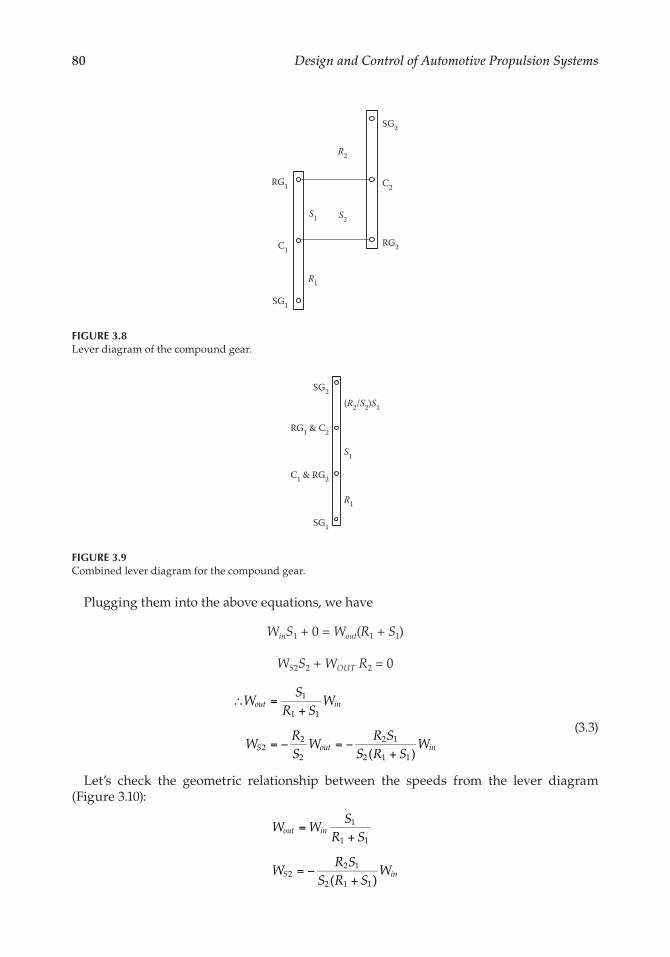
80 Design and Control of Automotive Propulsion Systems
Plugging them into the above equations, we have
WinS1 + 0 = Wout(R1 + S1)
WS2S2 + WOUT R2 = 0
∴ =+
= − = −+( )
1
1 1
22
2
2 1
2 1 1
WS
R SW
WRS
WR S
S R SW
out in
S out in
(3.3)
Let’s check the geometric relationship between the speeds from the lever diagram (Figure 3.10):
( )
1
1 1
22 1
2 1 1
W WS
R S
WR S
S R SW
out in
S in
=+
= −+
RG1
C1
SG1
SG2
C2
RG2
R2
S2S1
R1
FIGURE 3.8Lever diagram of the compound gear.
SG2(R2/S2)S1
R1
S1
C1 & RG2
SG1
RG1 & C2
FIGURE 3.9Combined lever diagram for the compound gear.

81Design, Modeling, and Control of Automotive Transmission Systems
Now let’s calculate the torque relationship at first gear (Figure 3.11):
Tin (R1 + S1) = Tout S1
TC2 = Tin − Tout
1 1
1
21 1
1
1
1
∴ =+
= −+
=
T TR S
S
T TR S
ST
RS
T
out in
C in in in
(3.4)
The lever diagram for the second gear is shown in Figure 3.12. Using similar methods as for the first gear, we can calculate the speed ratio for the second gear:
1 1 2 1 2
1 2 1 2
1 2 1 2 2 1
1 2 2 1
WW
R S R S SS R S S
WW
R S S S R SS S R S
in
out
in
out
=+ ++
=+ ++
SG2
(R2/S2)S1
R1
S1
C1 & RG2
SG1
RG1 & C2
Win
Wout
FIGURE 3.10Speed calculation for the compound gear.
SG2
TC2
R1
S1
C1 & RG2
SG1
RG1 & C2
Tin
Tout
FIGURE 3.11Torque calculation for the compound gear.

82 Design and Control of Automotive Propulsion Systems
Similarly, the lever diagram for the third gear is shown in Figure 3.13.
Wout = Win
The lever diagram for the fourth gear is shown in Figure 3.14.
2 1
2
21
21
2 1
2 1 1 2
2
2 2
WW
R SS
RSS
S
R SR S S S
RR S
in
out=
+=
+=
+
The lever diagram for the reverse gear is shown in Figure 3.15.
2 1
2
1
2
2
WW
R SSS
RS
in
out= − = −
The torque ratio can be calculated similarly. Also, given the conservation of energy, the torque ratio will be the inverse of the speed ratio. Recall T
TS
R Sin
out
1
1 1=
+ for the first gear.
SG2
(R2/S2)S1
R1
S1
C1 & RG2
SG1
RG1 & C2
Win
Wout
Second Gear
FIGURE 3.12Lever diagram for second gear.
SG2
R1
S1
C1 & RG2
SG1
RG1 & C2
Win
Wout
�ird Gear
Win
FIGURE 3.13Lever diagram for third gear.
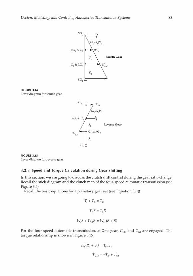
83Design, Modeling, and Control of Automotive Transmission Systems
3.2.3 Speed and Torque Calculation during Gear Shifting
In this section, we are going to discuss the clutch shift control during the gear ratio change. Recall the stick diagram and the clutch map of the four-speed automatic transmission (see Figure 3.5).
Recall the basic equations for a planetary gear set (see Equation (3.1)):
Ts + TR = TC
TRS = TSR
WsS + WRR = WC (R + S)
For the four-speed automatic transmission, at first gear, C123 and C1R are engaged. The torque relationship is shown in Figure 3.16.
Tin (R1 + S1) = ToutS1
TC1R = −Tin + Tout
SG2
(R2/S2)S1
R1
S1
C1 & RG2
SG1
RG1 & C2
Win
Wout
Reverse Gear
FIGURE 3.15Lever diagram for reverse gear.
SG2
(R2/S1)S2
R1
S1
C1 & RG2
SG1
RG1 & C2 Win
Wout
Fourth Gear
FIGURE 3.14Lever diagram for fourth gear.

84 Design and Control of Automotive Propulsion Systems
1 1
1
11
1
∴ =+
=
T TR S
S
TRS
T
out in
C R in
Now if we shift from first gear to second gear, clutch C24 is engaged and clutch C1R is disengaged. There is a time period where both clutch C24 and clutch C1R are interacting with the planetary gear set as shown in Figure 3.17.
TC24 + TC1R + Tin = Tout
( )
1
242 1
21 1 1
1 1
124
2
2
1 241
124
2
2
+ = +
∴ =+
−
= − − = − +
TR SS
T S T R S
T TR S
ST
RS
T T T T TRS
TRS
C out in
out in C
C R out in C in C
S1
R1
SG1Tin
TC1R
Tout
SG2
RG1 & C2
C1 & RG2
FIGURE 3.16Torque for first gear.
S1
R1
SG1Tin
TC1R
Tout
SG2
RG1 & C2
C1 & RG2
(R2/S1)S2
TC24
FIGURE 3.17Torque during first to second gear shift.
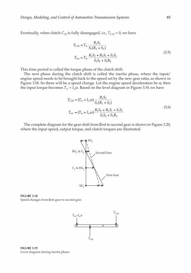
85Design, Modeling, and Control of Automotive Transmission Systems
Eventually, when clutch C1R is fully disengaged, i.e., TC1R = 0, we have
=+
=+ +
+
T TR S
S R S
T TR S R S S S
S S S R
C in
out in
( )241 2
1 2 2
1 2 2 1 1 2
1 2 1 2
(3.5)
This time period is called the torque phase of the clutch shift.The next phase during the clutch shift is called the inertia phase, where the input/
engine speed needs to be brought back to the speed set by the new gear ratio, as shown in Figure 3.18. So there will be a speed change. Let the engine speed deceleration be α; then the input torque becomes Tin + Iinα. Based on the level diagram in Figure 3.19, we have
= + α+
= + α+ +
+
T T IR S
S R S
T T IR S R S S S
S S S R
C in in
out in in
( )( )
( )
241 2
1 2 2
1 2 2 1 1 2
1 2 1 2
(3.6)
The complete diagram for the gear shift from first to second gear is shown in Figure 3.20, where the input speed, output torque, and clutch torques are illustrated.
Tin+Iinα
Tout
TC24
FIGURE 3.19Lever diagram during inertia phase.
SG1
SG2
RG1 & C2
C1 & RG2
First Gear
Second Gear
FIGURE 3.18Speed changes from first gear to second gear.
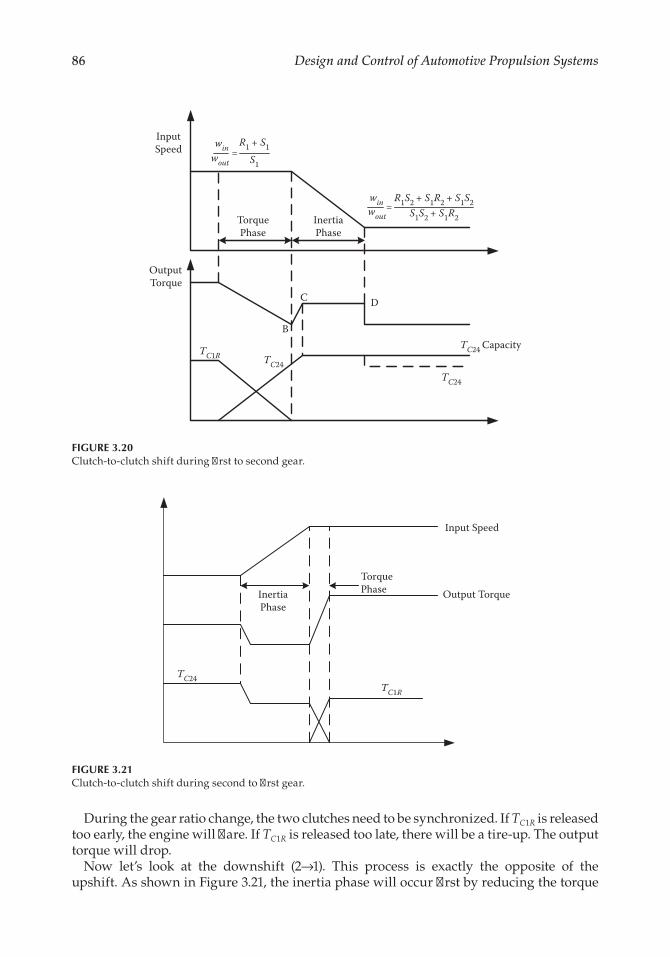
86 Design and Control of Automotive Propulsion Systems
During the gear ratio change, the two clutches need to be synchronized. If TC1R is released too early, the engine will flare. If TC1R is released too late, there will be a tire-up. The output torque will drop.
Now let’s look at the downshift (2→1). This process is exactly the opposite of the upshift. As shown in Figure 3.21, the inertia phase will occur first by reducing the torque
InputSpeed
OutputTorque
TorquePhase
InertiaPhase
TC24
TC24
B
C D
S1
R1 + S1wout
win =
S1S2 + S1R2
R1S2 + S1R2 + S1S2wout
win =
TC1RTC24 Capacity
FIGURE 3.20Clutch-to-clutch shift during first to second gear.
TC24TC1R
InertiaPhase
TorquePhase
Input Speed
Output Torque
FIGURE 3.21Clutch-to-clutch shift during second to first gear.

87Design, Modeling, and Control of Automotive Transmission Systems
on clutch C24, and the engine speed will rise to the speed set by the new gear ratio. Then the clutch torque for C24 will be reduced further and the torque for C1R will be increased in a synchronized fashion. This will complete the torque phase.
3.3 Design and Control of Transmission Clutches
From Section 3.2, it is clear that the gear ratios for automatic transmissions are realized by connecting different nodes of the planetary gear sets. This is achieved using electro-hydraulically actuated clutches. More importantly, for the clutch-to-clutch shift technol-ogy, where the oncoming clutch needs to be engaged and the offgoing clutch needs to be disengaged, synchronization between the two clutches is critical (see Figures 3.20 and 3.21). Therefore, clutch is a critical element of the transmission system, and its performance directly affects the overall functionality and performance of the transmission. This section will present the design, modeling, and control of transmission clutches.
3.3.1 Clutch Design
The commonly used clutch actuation devices in automatic transmissions are electro-hydraulically actuated clutches [1]. This is mainly due to the high power density of the fluid power system. A schematic diagram of a typical transmission clutch actuation system is shown in Figure 3.22 [1], while an illustration of the physical system is shown in Figure 3.23 [3]. When the clutch needs to be engaged, pressurized fluid flows into the clutch chamber and pushes the clutch piston toward the clutch packs until they are in contact. This process is called clutch fill. There is no torque transmission yet through the clutch at this stage. When the clutch is ready to transmit torque, the input pressure is further increased, which then squeezes the clutch packs with the clutch piston. The clutch packs are circular disks, and they are connected to different input and output shafts. Engagement of the clutch packs will enable the transfer of the engine torque to the vehicle driveline.
PistonSeal
Clutch Piston
ReturnSpring
Ori�ce
ClutchPacks
Ps
Pp
xp
FIGURE 3.22Schematic diagram of a clutch mechanism.

88 Design and Control of Automotive Propulsion Systems
For the clutch-to-clutch shift technology described in Section 3.2, it is imperative to control the clutch piston to reach the clutch packs within a specified clutch fill time because an improper clutch fill process can result in either an underfill or an overfill [2], both of which can cause the failure of the clutch shift synchronization, and therefore negatively affect the clutch shift quality. Underfill refers to the case where the clutch piston has not reached the clutch packs at the end of the clutch fill process. So the clutch is not ready for engagement when it is supposed to be. Overfill refers to the case where the clutch piston has traveled more than required and started to squeeze the clutch packs at the end of the clutch fill process. This will start torque transmission prematurely. The clutch engagement process will see a significant pressure rise by squeezing on the clutch packs to transmit torque. The smooth and synchronized torque transmission is critical for shift and drive quality. In the following sections, several different methods will be introduced to control the clutch fill and engagement processes.
3.3.2 New Clutch Actuation Mechanism
In this section, we show a new clutch design that will automatically achieve precise clutch fill control [3]. Figure 3.24(a) [3] shows the simplified schematic diagram of the clutch actuation system, which mainly consists of two on/off valves, an internal feedback spool (IFS), an IFS return spring, a feedback channel, and the clutch assembly. The IFS controls the opening orifice between the supply pressure and the clutch chamber, and is the key component of the clutch actuation mechanism.
The following is the operating procedure of the system:
1. When the clutch piston is at the initial disengaged position (Figure 3.24(a)), on/off valve 1 connects the IFS orifice, AIFS, to the fluid tank. The pressure inside the clutch chamber is low, so the clutch piston will be kept at the disengaged position by the piston return spring.
2. When the clutch fill process begins, on/off valve 1 is energized to connect the IFS orifice to the supply pressure. Pressurized fluid then enters the clutch chamber through the IFS orifice, overcomes the spring force, and pushes the clutch piston to the right. On the other side, on/off valve 2 at the feedback exhaust port is closed
SealFluid Inlet
Piston
ClutchChamber
Orice
Rotational Axis(center of shaft)
Clutch Pack
Spring
Ball Capsule
FIGURE 3.23Physical illustration of a clutch mechanism.
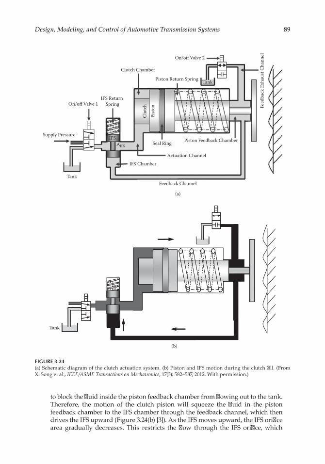
89Design, Modeling, and Control of Automotive Transmission Systems
to block the fluid inside the piston feedback chamber from flowing out to the tank. Therefore, the motion of the clutch piston will squeeze the fluid in the piston feedback chamber to the IFS chamber through the feedback channel, which then drives the IFS upward (Figure 3.24(b) [3]). As the IFS moves upward, the IFS orifice area gradually decreases. This restricts the flow through the IFS orifice, which
On/off Valve 1
On/off Valve 2
Clutch Chamber
Piston Return Spring Tank
Clut
chPi
ston
Supply Pressure
Tank
IFS Return Spring
IFS Chamber
Feedback Channel
(a)
Piston Feedback Chamber
Feed
back
Exh
aust
Cha
nnel
IFSAIFS Seal Ring
Actuation Channel
Tank
(b)
FIGURE 3.24(a) Schematic diagram of the clutch actuation system. (b) Piston and IFS motion during the clutch fill. (From X. Song et al., IEEE/ASME Transactions on Mechatronics, 17(3): 582–587, 2012. With permission.)

90 Design and Control of Automotive Propulsion Systems
then slows down the pressure rise in the clutch chamber. The regulated chamber pressure will again affect the clutch piston displacement, and therefore form a feedback loop. The clutch piston and the IFS continue to move in a synchronized fashion until the IFS orifice is cut off, which then separates the clutch chamber from the supply pressure, and the piston naturally stops at the predetermined position.
From the above analysis, it can be observed that the clutch piston displacement is fed back through the IFS orifice area, which regulates the fluid pressure inside the clutch chamber. The flow, pressure, and displacement are precisely coordinated by the embedded hydromechanical feedback loop. This internal feedback struc-ture ensures robust and precise motion of the clutch fill process. The feedback structure also guarantees a smoothly decreasing clutch piston velocity profile as it approaches the clutch fill final position.
3. After the clutch fill, the clutch packs are ready to be engaged for torque transmis-sion. When the clutch engagement starts, the clutch piston needs to be pushed further to squeeze the clutch packs. This can be realized by opening on/off valve 2 at the exhaust port to release the fluid in the feedback chamber to the tank. As a result, the pressures in the piston feedback chamber and the IFS chamber will drop, and subsequently the IFS return spring pushes the IFS downward until the IFS orifice is fully open. The supply pressure, Ps, which now gets reconnected to the clutch chamber, will push the clutch piston further to squeeze the clutch packs.
4. During the clutch disengagement, the clutch piston needs to move back to its initial position so that the clutch packs will be released. On/off valve 1 is deener-gized to connect the IFS orifice to the low-pressure tank. The piston return spring will then push the piston back to the disengaged position.
The control block diagram of the IFS clutch actuation system is shown in Figure 3.25 [3], which shows that the clutch mechanism consisting of the IFS, the clutch piston, and the on/off valve can be represented in a feedback loop.
There are two advantages of this new mechanism for clutch control. First, instead of designing a controller considering the complex nonlinear hydraulic dynamics, the pro-posed IFS clutch actuation system can realize a fast, precise, and robust nonlinear control by self-regulating the IFS spool orifice with the hydromechanical feedback rather than sensor measurement. The orifice area automatically regulates the clutch chamber pressure, and thus enables a smooth and precise clutch piston velocity and displacement profile.
Control Element(Spool Orifice)
Plant(Clutch)
PistonDisplacement
Feedback Element(Displacement Ratio)
SpoolDisplacement
Spool Opening
Area
FIGURE 3.25Feedback control diagram for the clutch mechanism. (From X. Song et al., IEEE/ASME Transactions on Mechatronics, 17(3): 582–587, 2012. With permission.)
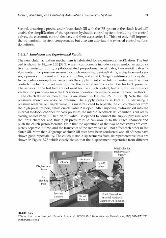
91Design, Modeling, and Control of Automotive Transmission Systems
Second, ensuring a precise and robust clutch fill with the IFS system at the clutch level will enable the simplification of the upstream hydraulic control system, including the control valves, the electronic control devices, and their accessories [4]. This not only will improve the transmission system compactness, but also can alleviate the external control calibra-tion efforts.
3.3.2.1 Simulation and Experimental Results
The new clutch actuation mechanism is fabricated for experimental verification. The test bed is shown in Figure 3.26 [3]. The main components include a servo motor, an automo-tive transmission pump, a pilot-operated proportional relief valve, two on/off valves, a flow meter, two pressure sensors, a clutch mounting device/fixture, a displacement sen-sor, a power supply unit with servo amplifier, and an xPC Target real-time control system. In particular, one on/off valve controls the supply oil into the clutch chamber, and the other controls the hydraulic oil injection into the internal feedback chamber for back pressure. The sensors in the test bed are not used for the clutch control, but only for performance verification purposes since the IFS system operation requires no measurement feedback.
The clutch fill experimental results are shown in Figures 3.27 to 3.30 [3]. Note that the pressures shown are absolute pressure. The supply pressure is kept at 12 bar using a pressure relief valve. On/off valve 1 is initially closed to separate the clutch chamber from the high-pressure port, while on/off valve 2 is open. After injecting hydraulic oil into the internal feedback channel for back pressure, the internal feedback IFS chamber is cut off by closing on/off valve 2. Then on/off valve 1 is opened to connect the supply pressure with the input chamber, and thus high-pressure fluid can flow in to the clutch chamber and push the clutch piston forward. Note that the operations of the two on/off valves are com-pletely separate in time, and the transients of the two valves will not affect each other in the clutch fill. More than 30 groups of clutch fill tests have been conducted, and all of them have shown good repeatability. The clutch piston displacements from six representative tests are shown in Figure 3.27, which clearly shows that the displacement trajectories from different
Relief Valve forHigh Pressure
Supply
Fluid Channel forInternal Feedback
Chamber Oil Injection
Displacement Sensor
PressureSensors
IFS BodyClutch
AirBleeding
Port
On/o� Valve 1
On/o� Valve 2
FIGURE 3.26IFS clutch actuation test bed. (From X. Song et al., IEEE/ASME Transactions on Mechatronics, 17(3): 582–587, 2012. With permission.)
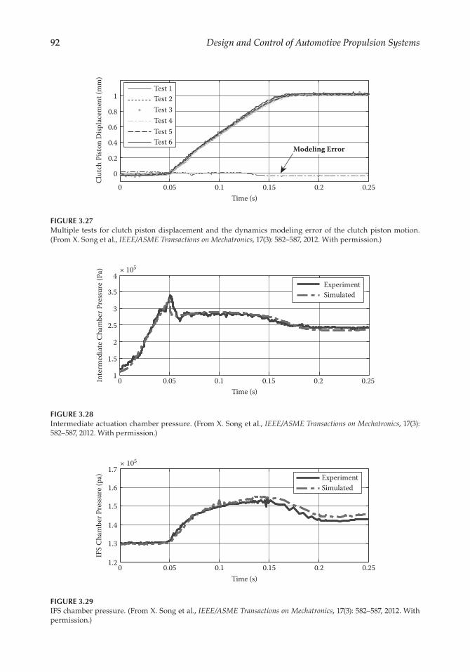
92 Design and Control of Automotive Propulsion Systems
0 0.05 0.1 0.15 0.2 0.25
0
0.2
0.4
0.6
0.8
1
Time (s)
Clut
ch P
iston
Disp
lace
men
t (m
m)
Test 1Test 2Test 3Test 4Test 5Test 6
Modeling Error
FIGURE 3.27Multiple tests for clutch piston displacement and the dynamics modeling error of the clutch piston motion. (From X. Song et al., IEEE/ASME Transactions on Mechatronics, 17(3): 582–587, 2012. With permission.)
0 0.05 0.1 0.15 0.2 0.251
1.5
2
2.5
3
3.5
4× 10⁵
Time (s)
Inte
rmed
iate
Cha
mbe
r Pre
ssur
e (Pa
)
ExperimentSimulated
FIGURE 3.28Intermediate actuation chamber pressure. (From X. Song et al., IEEE/ASME Transactions on Mechatronics, 17(3): 582–587, 2012. With permission.)
0 0.05 0.1 0.15 0.2 0.251.2
1.3
1.4
1.5
1.6
1.7× 10⁵
Time (s)
IFS
Cham
ber P
ress
ure (
pa) Experiment
Simulated
FIGURE 3.29IFS chamber pressure. (From X. Song et al., IEEE/ASME Transactions on Mechatronics, 17(3): 582–587, 2012. With permission.)
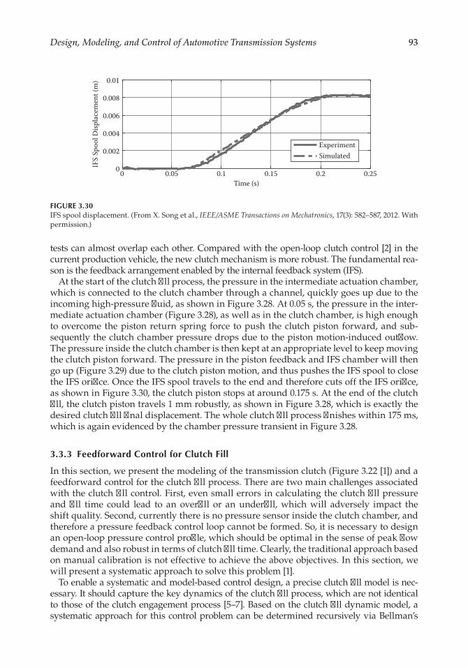
93Design, Modeling, and Control of Automotive Transmission Systems
tests can almost overlap each other. Compared with the open-loop clutch control [2] in the current production vehicle, the new clutch mechanism is more robust. The fundamental rea-son is the feedback arrangement enabled by the internal feedback system (IFS).
At the start of the clutch fill process, the pressure in the intermediate actuation chamber, which is connected to the clutch chamber through a channel, quickly goes up due to the incoming high-pressure fluid, as shown in Figure 3.28. At 0.05 s, the pressure in the inter-mediate actuation chamber (Figure 3.28), as well as in the clutch chamber, is high enough to overcome the piston return spring force to push the clutch piston forward, and sub-sequently the clutch chamber pressure drops due to the piston motion-induced outflow. The pressure inside the clutch chamber is then kept at an appropriate level to keep moving the clutch piston forward. The pressure in the piston feedback and IFS chamber will then go up (Figure 3.29) due to the clutch piston motion, and thus pushes the IFS spool to close the IFS orifice. Once the IFS spool travels to the end and therefore cuts off the IFS orifice, as shown in Figure 3.30, the clutch piston stops at around 0.175 s. At the end of the clutch fill, the clutch piston travels 1 mm robustly, as shown in Figure 3.28, which is exactly the desired clutch fill final displacement. The whole clutch fill process finishes within 175 ms, which is again evidenced by the chamber pressure transient in Figure 3.28.
3.3.3 Feedforward Control for Clutch Fill
In this section, we present the modeling of the transmission clutch (Figure 3.22 [1]) and a feedforward control for the clutch fill process. There are two main challenges associated with the clutch fill control. First, even small errors in calculating the clutch fill pressure and fill time could lead to an overfill or an underfill, which will adversely impact the shift quality. Second, currently there is no pressure sensor inside the clutch chamber, and therefore a pressure feedback control loop cannot be formed. So, it is necessary to design an open-loop pressure control profile, which should be optimal in the sense of peak flow demand and also robust in terms of clutch fill time. Clearly, the traditional approach based on manual calibration is not effective to achieve the above objectives. In this section, we will present a systematic approach to solve this problem [1].
To enable a systematic and model-based control design, a precise clutch fill model is nec-essary. It should capture the key dynamics of the clutch fill process, which are not identical to those of the clutch engagement process [5–7]. Based on the clutch fill dynamic model, a systematic approach for this control problem can be determined recursively via Bellman’s
0 0.05 0.1 0.15 0.2 0.250
0.002
0.004
0.006
0.008
0.01
Time (s)
IFS
Spoo
l Disp
lace
men
t (m
)
ExperimentSimulated
FIGURE 3.30IFS spool displacement. (From X. Song et al., IEEE/ASME Transactions on Mechatronics, 17(3): 582–587, 2012. With permission.)

94 Design and Control of Automotive Propulsion Systems
dynamic programming (DP) method [8, 9]. However, different from other applications, the clutch actuation system contains high frequency and stiff dynamics [6, 7], which requires a very fast sampling rate for the discretized model. As a result, the large number of steps, along with the curse of dimensionality [10] associated with conventional numerical DP method, pro-hibits its efficient implementation for the clutch fill control problem. Furthermore, the conven-tional numeric DP algorithm suffers from interpolation errors, which will affect the accuracy of the final results. Therefore, we will show a customized numerical dynamic programming approach, which has successfully solved the above problems and generated satisfactory results. The customized DP method transforms the stiff dynamic model into a nonstiff one by a unique model structure transformation and state discretization, and thus enables the reduc-tion of the discrete sampling steps. Furthermore, by discretizing the state space into regions rather than discrete nodes, the interpolation error is avoided. Finally, the customized DP only searches the optimal solution within the reachable discrete states, which dramatically reduces the searching space and therefore mitigates the curse of the dimensionality problem [10].
3.3.3.1 Clutch System Modeling
As shown in Figure 3.22, ps is the supply pressure command and also the control input to the system, pp is the pressure inside the clutch chamber, and xp is the clutch piston displacement. The pressurized fluid flows into the clutch chamber and pushes the clutch piston to the right, and finally contacts the clutch packs. The dynamics associated with clutch fill can be modeled as [1]
1 2x x=� (3.7)
1
[ ( ) ( , ) ( )]2 3 2 3 2 1 0xM
A x P P D x F x P x K x xp
p c atm p drag c p p= × + − − − + − × +� (3.8)
( )2| |
30 1
33
2=β+
−−ρ
−�xV A x
sign u x C Au x
A xp
d orifice p (3.9)
where
1
2
3
=
=
=
=
�
x x
x x
x p
u p
p
p
p
s
and
=
x
x
x u
(0)
(0)
(0)
0
0
(0)
1
2
3
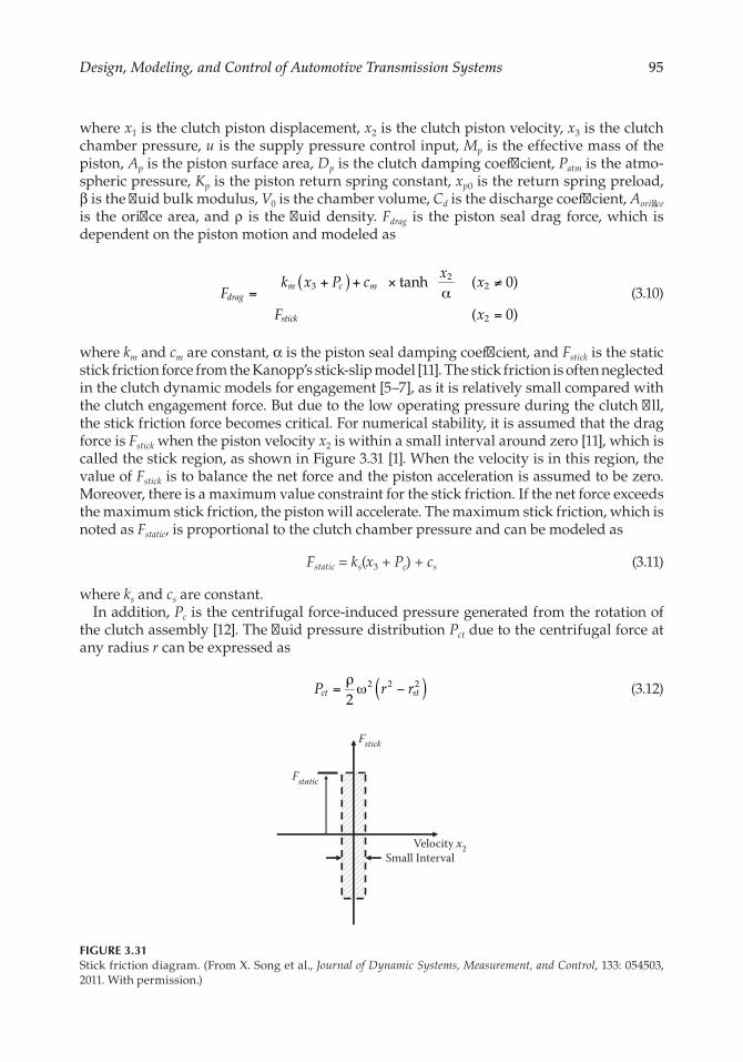
95Design, Modeling, and Control of Automotive Transmission Systems
where x1 is the clutch piston displacement, x2 is the clutch piston velocity, x3 is the clutch chamber pressure, u is the supply pressure control input, Mp is the effective mass of the piston, Ap is the piston surface area, Dp is the clutch damping coefficient, Patm is the atmo-spheric pressure, Kp is the piston return spring constant, xp0 is the return spring preload, β is the fluid bulk modulus, V0 is the chamber volume, Cd is the discharge coefficient, Aorifice is the orifice area, and ρ is the fluid density. Fdrag is the piston seal drag force, which is dependent on the piston motion and modeled as
tanh ( 0)
( 0)
32
2
2
( )=
+ + ×α
≠
=
Fk x P c
xx
F xdrag
m c m
stick
(3.10)
where km and cm are constant, α is the piston seal damping coefficient, and Fstick is the static stick friction force from the Kanopp’s stick-slip model [11]. The stick friction is often neglected in the clutch dynamic models for engagement [5–7], as it is relatively small compared with the clutch engagement force. But due to the low operating pressure during the clutch fill, the stick friction force becomes critical. For numerical stability, it is assumed that the drag force is Fstick when the piston velocity x2 is within a small interval around zero [11], which is called the stick region, as shown in Figure 3.31 [1]. When the velocity is in this region, the value of Fstick is to balance the net force and the piston acceleration is assumed to be zero. Moreover, there is a maximum value constraint for the stick friction. If the net force exceeds the maximum stick friction, the piston will accelerate. The maximum stick friction, which is noted as Fstatic, is proportional to the clutch chamber pressure and can be modeled as
Fstatic = ks(x3 + Pc) + cs (3.11)
where ks and cs are constant.In addition, Pc is the centrifugal force-induced pressure generated from the rotation of
the clutch assembly [12]. The fluid pressure distribution Pct due to the centrifugal force at any radius r can be expressed as
2
2 2 2P r rct st( )=ρω − (3.12)
Fstatic
Fstick
Small IntervalVelocity x2
FIGURE 3.31Stick friction diagram. (From X. Song et al., Journal of Dynamic Systems, Measurement, and Control, 133: 054503, 2011. With permission.)
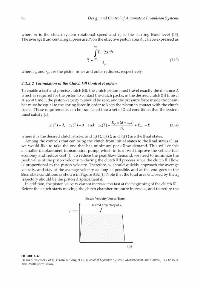
96 Design and Control of Automotive Propulsion Systems
where ω is the clutch system rotational speed and rst is the starting fluid level [13]. The average fluid centrifugal pressure Pc on the effective piston area Ap can be expressed as
2∫=
⋅ π
P
P rdr
Ac
ct
r
r
p
pi
po
(3.13)
where rpi and rpo are the piston inner and outer radiuses, respectively.
3.3.3.2 Formulation of the Clutch Fill Control Problem
To enable a fast and precise clutch fill, the clutch piston must travel exactly the distance d, which is required for the piston to contact the clutch packs, in the desired clutch fill time T. Also, at time T, the piston velocity x2 should be zero, and the pressure force inside the cham-ber must be equal to the spring force in order to keep the piston in contact with the clutch packs. These requirements can be translated into a set of final conditions that the system must satisfy [1]:
= = =× +
+ −( ) , ( ) 0 and ( )( )
1 2 30x T d x T x T
K d xA
P Pp p
patm c (3.14)
where d is the desired clutch stroke, and x1(T), x2(T), and x3(T) are the final states.Among the controls that can bring the clutch from initial states to the final states (3.14),
we would like to take the one that has minimum peak flow demand. This will enable a smaller displacement transmission pump, which in turn will improve the vehicle fuel economy and reduce cost [4]. To reduce the peak flow demand, we need to minimize the peak value of the piston velocity x2 during the clutch fill process since the clutch fill flow is proportional to the piston velocity. Therefore, x2 should quickly approach the average velocity, and stay at the average velocity as long as possible, and at the end goes to the final state conditions as shown in Figure 3.32 [1]. Note that the total area enclosed by the x2 trajectory should be the piston displacement d.
In addition, the piston velocity cannot increase too fast at the beginning of the clutch fill. Before the clutch starts moving, the clutch chamber pressure increases, and therefore the
Piston Velocity Versus Time
x2 (m/s)
t (s)
Desired Trajectory of x2
FIGURE 3.32Desired trajectory of x2. (From X. Song et al., Journal of Dynamic Systems, Measurement, and Control, 133: 054503, 2011. With permission.)
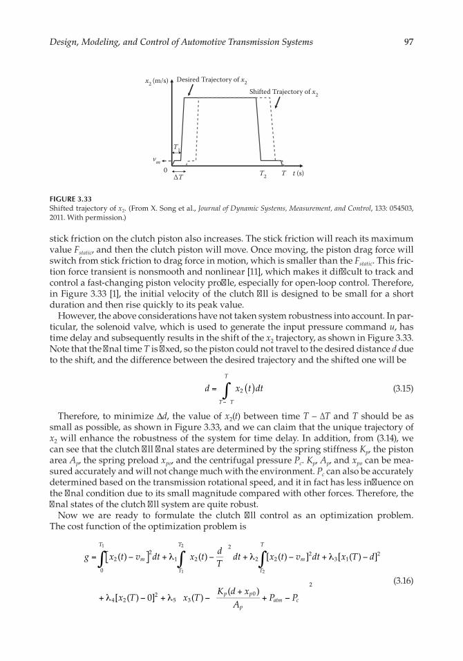
97Design, Modeling, and Control of Automotive Transmission Systems
stick friction on the clutch piston also increases. The stick friction will reach its maximum value Fstatic, and then the clutch piston will move. Once moving, the piston drag force will switch from stick friction to drag force in motion, which is smaller than the Fstatic. This fric-tion force transient is nonsmooth and nonlinear [11], which makes it difficult to track and control a fast-changing piston velocity profile, especially for open-loop control. Therefore, in Figure 3.33 [1], the initial velocity of the clutch fill is designed to be small for a short duration and then rise quickly to its peak value.
However, the above considerations have not taken system robustness into account. In par-ticular, the solenoid valve, which is used to generate the input pressure command u, has time delay and subsequently results in the shift of the x2 trajectory, as shown in Figure 3.33. Note that the final time T is fixed, so the piston could not travel to the desired distance d due to the shift, and the difference between the desired trajectory and the shifted one will be
∫ ( )=−
d x t dtT T
T
2 (3.15)
Therefore, to minimize Δd, the value of x2(t) between time T – ΔT and T should be as small as possible, as shown in Figure 3.33, and we can claim that the unique trajectory of x2 will enhance the robustness of the system for time delay. In addition, from (3.14), we can see that the clutch fill final states are determined by the spring stiffness Kp, the piston area Ap, the spring preload xpo, and the centrifugal pressure Pc. Kp, Ap, and xpo can be mea-sured accurately and will not change much with the environment. Pc can also be accurately determined based on the transmission rotational speed, and it in fact has less influence on the final condition due to its small magnitude compared with other forces. Therefore, the final states of the clutch fill system are quite robust.
Now we are ready to formulate the clutch fill control as an optimization problem. The cost function of the optimization problem is
∫ ∫ ∫[ ]= − + λ − + λ − + λ −
+ λ − + λ −+
+ −
( ) ( ) [ ( ) ] [ ( ) ]
[ ( ) 0] ( )( )
22
0
1 2
2
2 22
3 12
4 22
5 30
2
1
1
2
2
g x t v dt x tdT
dt x t v dt x T d
x T x TK d x
AP P
m
T
T
T
m
T
T
p p
patm c
(3.16)
x2 (m/s)
t (s)
Desired Trajectory of x2
T
Shifted Trajectory of x2
T20
T1
vm
∆T
FIGURE 3.33Shifted trajectory of x2. (From X. Song et al., Journal of Dynamic Systems, Measurement, and Control, 133: 054503, 2011. With permission.)
98 Design and Control of Automotive Propulsion Systems
In particular, the first term of the cost function ensures the piston to start with a low velocity vm. The second term ensures that the velocity x2 remains close to the average veloc-ity d/T, which will minimize the peak value of x2, and therefore the peak flow demand. The third term ensures x2 to be as small as possible (close to zero) from time T2 to final time T, which will enhance system robustness. The last three terms ensures that the system will reach the specified final conditions in the required time T. λ1, λ2, λ3, λ4, and λ5 are the weighting factors.
3.3.3.3 Optimal Control Design
A systematic solution to the above optimization problem can be determined recursively via Bellman’s dynamic programming. Since the system model (Equations (3.7) to (3.9)) is nonlinear, an analytical solution cannot be obtained. Instead, a numerical solution will be provided. But first we need to discretize the system model to carry out the numerical dynamic programming method.
3.3.3.3.1 System Model Discretization
We discretize the system model (Equations (3.7) to (3.9)) as follows [1]:
x1(k + 1) = Δtx2(k) + x1(k) (3.17)
}
{ ( ) ( )
( )
+ = + + − −
− + − × +
( 1) ( ) [ ]
, ( ) [ ( ) ]
2 2 3 2
3 2 1 0
x k x kt
MA x k P P D x k
F x k P x k K x k x
pp c atm p
drag c p p
(3.18)
1 ( )2 ( )
30 1
33
2
3
( )( )
( )( )
( )
( )
+ =β
+− ×
−
ρ−
+
x kt
V A x ksign u k x k C A
u k x kA x k
x k
pd orifice p
(3.19)
where Δt refers to the sampling time. For simplicity, define f as the simple representation of the state space model (Equations (3.17) to (3.19)), and define X(k) = [x1(k), x2(k), x3(k)]T.
We define N = T/Δt as the number of steps from the initial state to the final state. And the cost function (3.16) becomes
∑ ∑ ∑= − + λ − + λ −
+λ − + λ − + λ −+
+ −
= = + = +
−
g X x k v t x kdT
t x k v t
x N d x N x NK d x
AP P
m
k
N
k N
N
m
k N
N
p p
patm c
( ) [ ( ) ] ( ) [ ( ) ]
[ ( ) ] [ ( ) 0] ( )( )
22
0
1 2
2
1
2 22
1
1
3 12
4 22
5 30
2
1
1
2
2
(3.20)
Consequently, the optimal control problem is to find an optimal control input u to minimize the cost function
( ) min ( )J X g Xu U
=∈
(3.21)
99Design, Modeling, and Control of Automotive Transmission Systems
where X = [X(0), …, X(N)], u = [u(0), …, u(N)], and U represents the set of feasible control inputs.
3.3.3.3.2 Optimal Control Using a Customized Dynamic Programming Method
First, it is desirable to avoid the stiffness and sampling interval constraint associated with the clutch fill dynamic model. One possible way to realize this is to have a proper trans-formation of the model structure, and therefore change its stiff characteristic. Given the structure of the system model (Equations (3.17) to (3.19)), if x1(k + 1), x2(k + 1), x3(k + 1), and x2(k) are known, we can calculate the values of x1(k), x3(k), and the input u(k) as follows:
x1(k) = x1(k + 1) − Δtx2(k) = R1(k) (3.22)
x3(k) = R2(k) (3.23)
( ) ( )2
( )2
3 3( )=ρ+ =u k sign W
WC A
x k R kd orifice
(3.24)
where
13 3
0 12( ) ( )
( )( )= + − ×
+
β+W x k x k
V A x k
tA x k
pp
The equation R2(k) determines the chamber pressure x3(k) in the step k and involves the drag force Fdrag term, which has different models depending on the piston velocity x2. When x2(k) is not zero, Fdrag can be obtained from Equation (3.10) and R2(k) is
( )( ) ( )
( ) ( ) ( )
=
− ×α
× + − ×
− − + + + + +α
( )1
tanh1
( ) ( )tanh
22
2 2
2 1 02
R kA k
x kx k x k
Mt
A P P D x k K x k x c k Px k
p m
p
p c atm p p p m m c
When x2(k) is zero but x2(k + 1) is nonzero, which means that the piston starts moving, the Fdrag is assumed to be the maximum static friction Fstatic in (3.11) and R2(k) becomes
( )1
1
( ) ( )
2 2 2
2 1 0 }
{ ( ) ( )
( ) ( )
=−
× + − ×
− − + + + + +
R kA k
x k x kM
t
A P P D x k K x k x c k P
p s
p
p c atm p p p s s c
When both x2(k) and x2(k + 1) are zero, which means that the piston stays static, the chamber pressure x3(k) variation is assumed to be small and R2(k) becomes
R2(k) = x3(k + 1)
100 Design and Control of Automotive Propulsion Systems
For notation simplicity, we can denote Equations (3.22), (3.23), and (3.24) as [x1(k), x3(k), u(k)] = R[x1(k + 1), x2(k + 1), x3(k + 1), x2(k)]. Note that as x2(k) is now predetermined in the inverse dynamic model (Equations (3.22) to (3.24)), it could be regarded as an input, and the new unknown states become [x1(k), x3(k), u(k)]. Therefore, the Jacobian matrix of (Equations (3.22) to (3.24)) becomes
R k R k R kx k x k u k
R kx k
R kx k
R kx k
T
T
[ ( ), ( ), ( )][ ( 1), ( 1), ( 1)]
1 0 0( )
( 1)0 0
( )( 1)
( )( 1)
0
1 2 3
1 3
2
1
3
1
3
3
∂∂ + + +
=
∂∂ +
∂∂ +
∂∂ +
(3.25)
The eigenvalues of (3.25) are always inside or on the unit circle regardless of the value of Δt, which means the dynamic model (Equations (3.22) to (3.24)) is not stiff [14], and therefore the sampling interval constraint can be avoided. Note that the above model transformation still requires the predetermined value for x1(k + 1), x2(k + 1), x3(k + 1), and x2(k). Interestingly, as the dynamic programming is implemented in a backward fashion, x1(k + 1), x2(k + 1), and x3(k + 1) were calculated in the previous step, and x2(k) can be dis-cretized into finite grids and predetermined in advance. Note that not all model inversion will result in nonstiff dynamics. For example, the inverse model X(k) = X(k + 1) – f[X(k + 1), u(k)] × Δt ( f is the dynamic model (Equations (3.17) to (3.19))) using the backward Euler method is still stiff [15].
Therefore, instead of making combinations of predetermined discrete values of x1(k), x2(k), and x3(k) in the conventional DP [16], we only need to generate the predetermined discrete values for x2(k) at each step, and then use the values of x1(k + 1), x2(k + 1), and x3(k + 1) from the previous step, together with x2(k), to obtain the values for x1(k) and x3(k). Consequently, unlike the conventional DP, which searches the entire discrete state space [16], the states to search are determined by the system dynamics (Equations (3.22) to (3.24)), and therefore all the discrete states searched in the DP computation are reachable.
However, although the discrete states generated by the above method are all reach-able, the number of discrete states will increase from step to step. Suppose the number of discrete states at step k + 1 is Lk+1, and the number of discrete values of x2(k) at step k is L, then the total number of discrete states generated for step k would be Lk = Lk+1 × L. So the number of states will grow very quickly after N steps. To avoid this problem, instead of discretizing the state space into specific discrete values, the customized dynamic pro-gramming algorithm divides the state space into several regions. As shown in Figure 3.34 [1], 2
0{ )(x k , 21 ( )x k , …, 2 ( )x kj , …, 2 })(x kL are the discrete values of x2 at step k, and {X0(k + 1),
X1(k + 1), …, Xi(k + 1), …, XLk+1(k + 1)} are the possible discrete states calculated from step k + 1. In addition, for each discrete value of x2(k), we can generate several discrete regions on the plane of x1 and x3, shown as the black and white blocks in Figure 3.34. Then sup-pose from
( ) ( ) = +x k x k u k R X k x ki i i i j, , ( ) ( 1), ( )1 3 2 (3.26)
we get 1 ( )x ki and 3( )x ki , and suppose that , ,1 2 3( ) ( ) ( )x k x k x ki j i T lies in region A in Figure 3.34.
Subsequently, we can assign the vector , ,1 2 3( ) ( ) ( )x k x k x ki j i T as the value of region A, and

101Design, Modeling, and Control of Automotive Transmission Systems
also memorize , ,1 2 3( ) ( ) ( )x k x k x ki j i T as one of the discrete states for step k. Moreover, we can
calculate the cost function based on , ,1 2 3( ) ( ) ( )x k x k x ki j i T as
( ), ( ), ( ) ( ) ˆ ( 1)1 2 3 2
21= λ − + ++J x k x k x k x k v J X kk
i j ie
jk
i (3.27)
where ˆ1Jk+ is the cost function of state Xi(k + 1) at step k + 1. Here we also define two
symbols v and λe, which are equal to vm in (3.16) and 1, respectively, when step k ≤ N1; d/T and λ1, respectively, when step k ≤ N2; and vm and λ2, respectively, when k > N2.
In the following calculation, if , ,1 2 3( ) ( ) ( )+ +x k x k x ki c j i c T obtained from 1 ,1 2( ) ( )++R X k x ki c j
also lies in region A, we then calculate the cost function again based on , ,1 2( ) ( )+x k x ki c j
3 ( )+x ki c T as
( ), ( ), ( ) ( ) ˆ ( 1)1 2 3 2
21= λ − + ++ +
++J x k x k x k x k v J X kk
i c j i ce
jk
i c (3.28)
If , ,1 2 3( ) ( ) ( )J x k x k x kki j i is larger than , , ,1 2 3( ) ( ) ( )+ +J x k x k x kk
i c j i c we should reassign the
value of region A as , , ,1 2 3( ) ( ) ( )+ +x k x k x ki c j i c T and at the same time , ,1 2 3( ) ( ) ( )x k x k x ki j i T
in
the discrete space will be replaced by , , .1 2 3( ) ( ) ( )+ +x k x k x ki c j i c T But if , ,1 2 3( ) ( ) ( )J x k x k x kk
i j i is
smaller than , , ,1 2 3( ) ( ) ( )+ +J x k x k x kki c j i c , ,1 2 3( ) ( ) ( )+ +x k x k x ki c j i c T
will be disregarded and the process goes on.
We summarize the customized dynamic programming algorithm as follows: First, x2(k) is discretized into a finite grid with size L, and the x1 and x3 plane corresponding to each discrete x2
j(k) is discretized into L × L regions.
{ }
{ }
∈
∈ ×
x k x k x k x k x k
region k reg k reg k reg k reg k
j L
j j j jh
jL L
( ) ( ), ( ), ..., ( ), ..., ( )
( ) ( ), ( ), ... ( ), ..., ( )
2 21
22
2 2
1 2
(3.29)
x1
x3
x2
x2L(K)
x2j(K)
x20(K)
x1
x1
x3
x3
…...
…...
…...
…...
A
X0(k+1)
Xi(k+1)
XLk+1(k+1)
Xi+c(k+1)
FIGURE 3.34State space quantization. (From X. Song et al., Journal of Dynamic Systems, Measurement, and Control, 133: 054503, 2011. With permission.)
102 Design and Control of Automotive Propulsion Systems
where regionj(k) refers to the discrete regions on the x1− x3 plane corresponding to specific x2
j(k). Also, define λ as a diagonal matrix whose diagonal elements are the weighting factors λ3, λ4, and λ5 in Equation (3.20).
Step N – 1, for 1 ≤ j ≤ L:
( ) ( )− − − = −x N x N u N R X final x Nj1 , 1 , ( 1) _ , ( 1)1 3 2 (3.30)
( ) ( )− = − − −X N x N x N x Nj j( 1) 1 , ( 1), 11 2 3 (3.31)
[ ( 1)] [ ( 1) ]
[ ( 1), ( 1)] ( 1), ( 1)
1 2 22
{{ } }
− = λ − −
+ − − − λ − − −
−J X N x N v
f X N u N X f X N u N X
Nj j
m
jfinal
T jfinal
(3.32)
Step k, for 0 ≤ k < N – 1, for 1 ≤ j ≤ L, and for 1 ≤ i ≤ Lk+1:
( ) ( ) = +x k x k u k R X k x ki j, ( ), ( 1), ( )1 3 2 (3.33)
( ) ( )=X x k x k x ktempj, ( ),1 2 3 (3.34)
If ( )X reg ktemp jh∈ , then
= λ − + ++J x k v J X kk temp ej
ki( ) ( 1)_ 2
21 (3.35)
If [ ( ), ( )]_ 2J J x k reg kk temp kj
jh< , then
=J x k reg k Jkj
jh
k temp( ), ( )2 _ (3.36)
( ) ( )= =X k X x k x k x kjh
tempj( ) , ( ),1 2 3 (3.37)
Finally, after we have obtained the minimum cost function for each reachable state, we can easily get the optimal sequence of control input u = [u(0), …, u(N)], which would minimize the total cost function.
In summary, the above algorithm has three advantages over the conventional numerical DP algorithm. First, the system dynamic model is transformed from stiff equations into nonstiff equations. Thus, we can use a smaller number of steps (N = 800 for the simulation in Section 3.3.3.4) for DP. Second, all the states in the process are reachable, so by getting states x1(k) and x3(k) directly from x1(k + 1), x2(k + 1), x3(k + 1), and x2(k) using Equation (3.26), ˆ
1Jk+ in (3.27) can be directly matched with Jk+1[x1(k + 1), x2(k + 1), x3(k + 1)], therefore eliminating the approximation errors caused by interpolation in the conventional dynamic programming [16]. Third, as not all the discrete regions need to be considered during the process, the curse of dimensionality [10] problem is mitigated.
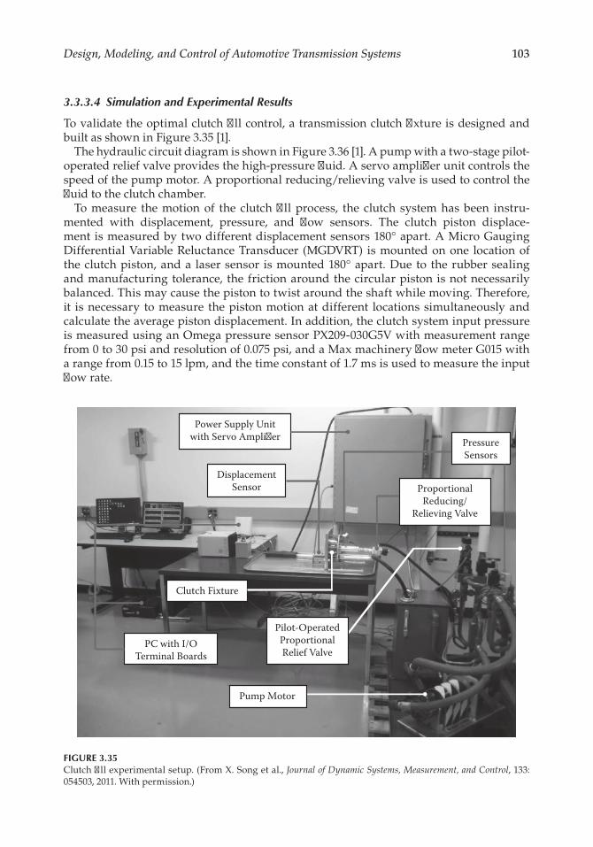
103Design, Modeling, and Control of Automotive Transmission Systems
3.3.3.4 Simulation and Experimental Results
To validate the optimal clutch fill control, a transmission clutch fixture is designed and built as shown in Figure 3.35 [1].
The hydraulic circuit diagram is shown in Figure 3.36 [1]. A pump with a two-stage pilot-operated relief valve provides the high-pressure fluid. A servo amplifier unit controls the speed of the pump motor. A proportional reducing/relieving valve is used to control the fluid to the clutch chamber.
To measure the motion of the clutch fill process, the clutch system has been instru-mented with displacement, pressure, and flow sensors. The clutch piston displace-ment is measured by two different displacement sensors 180° apart. A Micro Gauging Differential Variable Reluctance Transducer (MGDVRT) is mounted on one location of the clutch piston, and a laser sensor is mounted 180° apart. Due to the rubber sealing and manufacturing tolerance, the friction around the circular piston is not necessarily balanced. This may cause the piston to twist around the shaft while moving. Therefore, it is necessary to measure the piston motion at different locations simultaneously and calculate the average piston displacement. In addition, the clutch system input pressure is measured using an Omega pressure sensor PX209-030G5V with measurement range from 0 to 30 psi and resolution of 0.075 psi, and a Max machinery flow meter G015 with a range from 0.15 to 15 lpm, and the time constant of 1.7 ms is used to measure the input flow rate.
Power Supply Unitwith Servo Ampli�er
DisplacementSensor
Clutch Fixture
PC with I/OTerminal Boards
Pilot-OperatedProportionalRelief Valve
PressureSensors
ProportionalReducing/
Relieving Valve
Pump Motor
FIGURE 3.35Clutch fill experimental setup. (From X. Song et al., Journal of Dynamic Systems, Measurement, and Control, 133: 054503, 2011. With permission.)
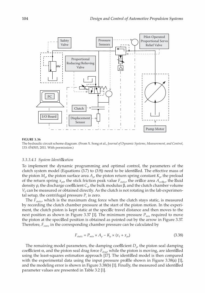
104 Design and Control of Automotive Propulsion Systems
3.3.3.4.1 System Identification
To implement the dynamic programming and optimal control, the parameters of the clutch system model (Equations (3.7) to (3.9)) need to be identified. The effective mass of the piston Mp, the piston surface area Ap, the piston return spring constant Kp, the preload of the return spring xp0, the stick friction peak value Fstatic, the orifice area Aorifice, the fluid density ρ, the discharge coefficient Cd, the bulk modulus β, and the clutch chamber volume V0 can be measured or obtained directly. As the clutch is not rotating in the lab experimen-tal setup, the centrifugal pressure Pc is zero.
The Fstatic, which is the maximum drag force when the clutch stays static, is measured by recording the clutch chamber pressure at the start of the piston motion. In the experi-ment, the clutch piston is kept static at the specific travel distance and then moves to the next position as shown in Figure 3.37 [1]. The minimum pressure Pmin required to move the piston at the specified position is obtained as pointed out by the arrow in Figure 3.37. Therefore, Fstatic in the corresponding chamber pressure can be calculated by
Fstatic = Pmin × Ap − Kp × (x1 + xpo) (3.38)
The remaining model parameters, the damping coefficient Dp, the piston seal damping coefficient α, and the piston seal drag force Fdrag, while the piston is moving, are identified using the least-squares estimation approach [17]. The identified model is then compared with the experimental data using the input pressure profile shown in Figure 3.38(a) [1], and the modeling error is shown in Figure 3.38(b) [1]. Finally, the measured and identified parameter values are presented in Table 3.2 [1].
Pilot-OperatedProportional Servo
Relief Valve
DisplacementSensor
Pump Motor
SafetyValve
ProportionalReducing/Relieving
Valve
Clutch
PressureSensors
I/O Board
PC
FIGURE 3.36The hydraulic circuit scheme diagram. (From X. Song et al., Journal of Dynamic Systems, Measurement, and Control, 133: 054503, 2011. With permission.)
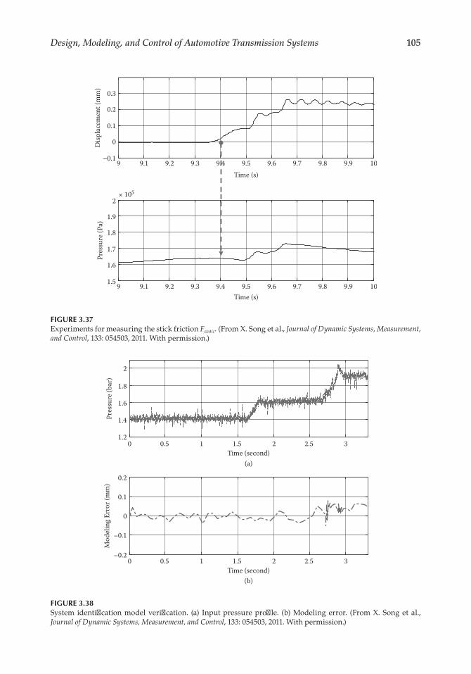
105Design, Modeling, and Control of Automotive Transmission Systems
0 0.5 1 1.5 2 2.5 31.2
1.4
1.6
1.8
2
Time (second)
Pres
sure
(bar
)
0 0.5 1 1.5 2 2.5 3–0.2
–0.1
0
0.1
0.2
Time (second)
(a)
(b)
Mod
elin
g Er
ror (
mm
)
FIGURE 3.38System identification model verification. (a) Input pressure profile. (b) Modeling error. (From X. Song et al., Journal of Dynamic Systems, Measurement, and Control, 133: 054503, 2011. With permission.)
9 9.1 9.2 9.3 9.4 9.5 9.6 9.7 9.8 9.9 10–0.1
0
0.1
0.2
0.3
Time (s)
Disp
lace
men
t (m
m)
9 9.1 9.2 9.3 9.4 9.5 9.6 9.7 9.8 9.9 101.5
1.6
1.7
1.8
1.9
2× 10⁵
Time (s)
Pres
sure
(Pa)
FIGURE 3.37Experiments for measuring the stick friction Fstatic. (From X. Song et al., Journal of Dynamic Systems, Measurement, and Control, 133: 054503, 2011. With permission.)

106 Design and Control of Automotive Propulsion Systems
3.3.3.4.2 Clutch Fill Simulation and Experimental Results
In this section, both simulation and experimental results are reported to validate the proposed control method. An optimal input pressure is derived to achieve the desired clutch fill velocity profile using the customized dynamic programming method. The desired final state conditions are x1(T) = d = 0.000725 (m), x2(T) = 0 (m/s), and x3(T) = 1.91 × 10⁵ (Pa). Figure 3.39 [1] (solid line) shows the optimal control input. The total steps for DP equal 800. The number of discrete values for x2(k) at each step is 100, and the number of discrete regions for each discrete x2(k) value is 100 × 100. For the customized DP method, we only evaluate the states that can be reached. The computation time for the customized DP method is 22 min with a 1.86 GHZ computer.
The resulting optimal control input pressure is then implemented in the experiment to verify its performance as shown in Figure 3.39 (dashed line). Due to the short time dura-tion (0.3 s) and total displacement (0.725 mm), precise pressure and motion control of the clutch fill process is very challenging. In addition, the clutch mechanism is extremely sen-sitive to pressure rise in the clutch chamber when the clutch piston starts to move, which adds up to the intricacy of controlling the clutch piston motion. This is because the current clutch design behaves as an on/off switch during the clutch fill process, where the input
TABLE 3.2
Parameter Values of the System Dynamic Model
Mp 0.4 (kg) T 0.3 (s)xp0 1.5928 (mm) Δt 0.000375 (s)Kp 242,640 (N/m) Aorifice 2.0442e-5 (m2)Dp 135.4 (N/m/s) ρ 880 (kg/m3)Ap 0.00628 (m2) Cd 0.7α 4.1054e-6 (m/s) Patm 1 (bar)V0 7.8e-5 (m3) β 1625 (bar)km 0.001517 (m2) ks 0.00153 (m2)cm 5.22 (N) cs 5.26 (N)
Source: X. Song et al., Journal of Dynamic Systems, Measurement, and Control, 133: 054503, 2011. With permission.
0 0.05 0.1 0.15 0.2 0.25 0.31.5
1.6
1.7
1.8
1.9
2
2.1
Time (second)
Pres
sure
(bar
)
Experimental pressureReference pressure from DP
FIGURE 3.39Optimal input pressure and the experimental tracking results. (From X. Song et al., Journal of Dynamic Systems, Measurement, and Control, 133: 054503, 2011. With permission.)

107Design, Modeling, and Control of Automotive Transmission Systems
pressure required to start the piston motion is only 0.3 bar lower than the final pressure (see Figure 3.39). Despite these challenges, the clutch piston displacement, velocity, and input flow profiles from the experiments exhibit optimal shape, as shown in Figure 3.40 [1]. The experimental velocity profile in Figure 3.40(b) is obtained by numerical differentiation of the displacement data, and its optimal shape can be further verified by the smooth input flow rate shown in Figure 3.40(c).
The repeatability issue is also verified using multiple experiments with the same desired pressure inputs shown in Figure 3.39. The experimental results in Figure 3.41 exhibit good repeatability. Specifically, Figure 3.41(a) presents the piston displacements from five groups of experiments, which clearly show that all the displacement trajectories have similar optimal shapes and can overlap each other. Figure 3.41(b) shows the error histo-gram of all the data points in the five trajectories compared with the desired one, which again exhibits good repeatability.
We also added ±5% and ±10% perturbations to the dynamic model parameters (Dp, α, β, Fdrag, ρ, Vo, Aorifice) and simulated the system performance using the designed control input in Figure 3.39. The trajectories shown in Figure 3.42 [1] arrived in acceptable intervals
0 0.05 0.1 0.15 0.2 0.25 0.30
0.2
0.4
0.6
0.8
(Time (second)(a)
(b)
(c)
Disp
lace
men
t (m
m) Experimental
Simulated from DP
0 0.05 0.1 0.15 0.2 0.25 0.30
2
4
6
Velo
city
(mm
/s)
Time (second)
0 0.05 0.1 0.15 0.2 0.25 0.30
1
2
3
4
5
Time (second)
Flow
Rat
e (l p
m)
FIGURE 3.40Experimental results for clutch displacement, velocity, and input flow rate. (From X. Song et al., Journal of Dynamic Systems, Measurement, and Control, 133: 054503, 2011. With permission.)
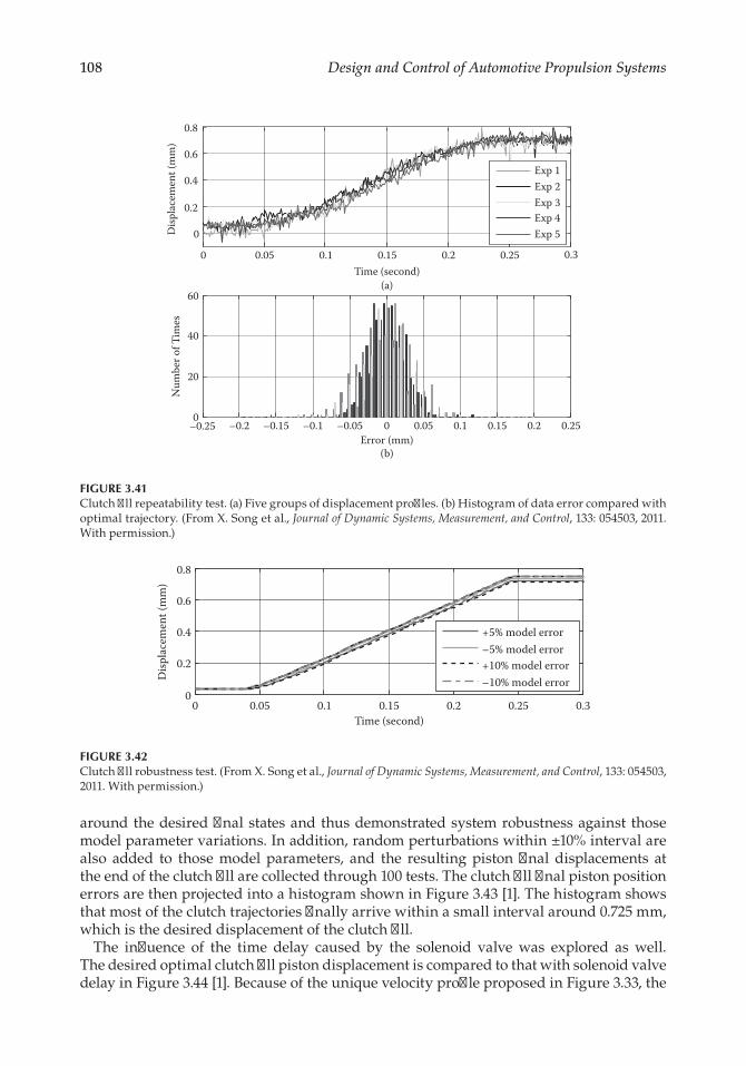
108 Design and Control of Automotive Propulsion Systems
around the desired final states and thus demonstrated system robustness against those model parameter variations. In addition, random perturbations within ±10% interval are also added to those model parameters, and the resulting piston final displacements at the end of the clutch fill are collected through 100 tests. The clutch fill final piston position errors are then projected into a histogram shown in Figure 3.43 [1]. The histogram shows that most of the clutch trajectories finally arrive within a small interval around 0.725 mm, which is the desired displacement of the clutch fill.
The influence of the time delay caused by the solenoid valve was explored as well. The desired optimal clutch fill piston displacement is compared to that with solenoid valve delay in Figure 3.44 [1]. Because of the unique velocity profile proposed in Figure 3.33, the
0 0.05 0.1 0.15 0.2 0.25 0.3
0
0.2
0.4
0.6
0.8
Time (second)(a)
(b)
Disp
lace
men
t (m
m)
Exp 1Exp 2Exp 3Exp 4Exp 5
–0.25 –0.2 –0.15 –0.1 –0.05 0 0.05 0.1 0.15 0.2 0.250
20
40
60
Error (mm)
Num
ber o
f Tim
es
FIGURE 3.41Clutch fill repeatability test. (a) Five groups of displacement profiles. (b) Histogram of data error compared with optimal trajectory. (From X. Song et al., Journal of Dynamic Systems, Measurement, and Control, 133: 054503, 2011. With permission.)
0 0.05 0.1 0.15 0.2 0.25 0.30
0.2
0.4
0.6
0.8
Time (second)
Disp
lace
men
t (m
m)
+5% model error–5% model error+10% model error–10% model error
FIGURE 3.42Clutch fill robustness test. (From X. Song et al., Journal of Dynamic Systems, Measurement, and Control, 133: 054503, 2011. With permission.)
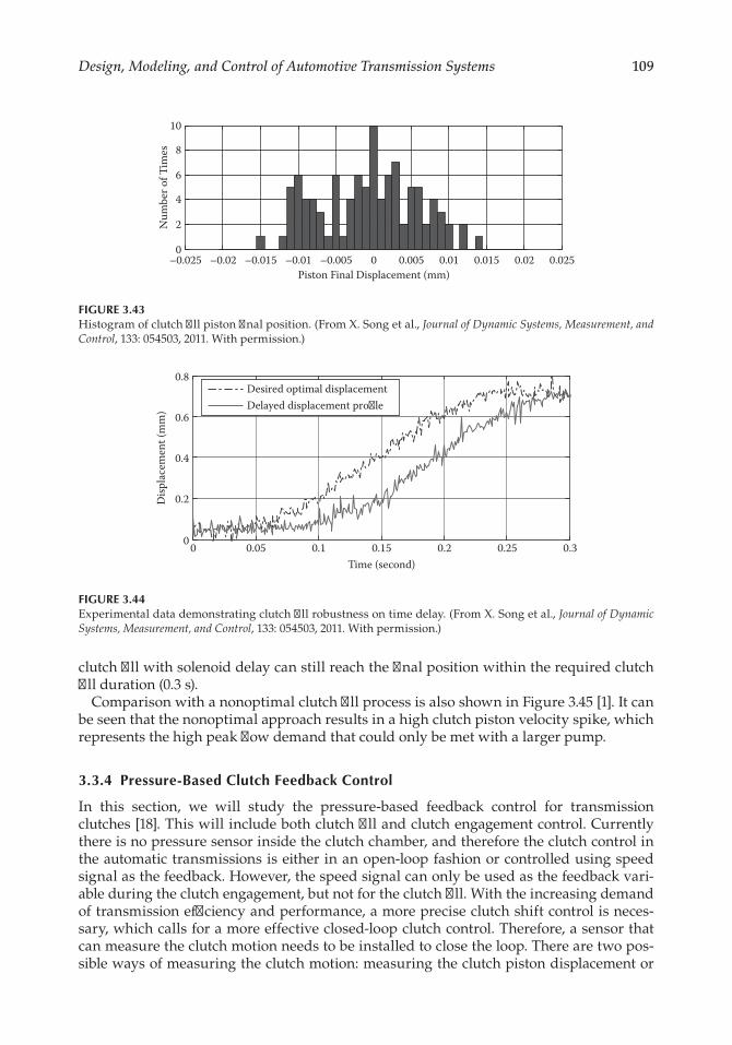
109Design, Modeling, and Control of Automotive Transmission Systems
clutch fill with solenoid delay can still reach the final position within the required clutch fill duration (0.3 s).
Comparison with a nonoptimal clutch fill process is also shown in Figure 3.45 [1]. It can be seen that the nonoptimal approach results in a high clutch piston velocity spike, which represents the high peak flow demand that could only be met with a larger pump.
3.3.4 Pressure-Based Clutch Feedback Control
In this section, we will study the pressure-based feedback control for transmission clutches [18]. This will include both clutch fill and clutch engagement control. Currently there is no pressure sensor inside the clutch chamber, and therefore the clutch control in the automatic transmissions is either in an open-loop fashion or controlled using speed signal as the feedback. However, the speed signal can only be used as the feedback vari-able during the clutch engagement, but not for the clutch fill. With the increasing demand of transmission efficiency and performance, a more precise clutch shift control is neces-sary, which calls for a more effective closed-loop clutch control. Therefore, a sensor that can measure the clutch motion needs to be installed to close the loop. There are two pos-sible ways of measuring the clutch motion: measuring the clutch piston displacement or
–0.025 –0.02 –0.015 –0.01 –0.005 0 0.005 0.01 0.015 0.02 0.0250
2
4
6
8
10
Piston Final Displacement (mm)
Num
ber o
f Tim
es
FIGURE 3.43Histogram of clutch fill piston final position. (From X. Song et al., Journal of Dynamic Systems, Measurement, and Control, 133: 054503, 2011. With permission.)
0 0.05 0.1 0.15 0.2 0.25 0.30
0.2
0.4
0.6
0.8
Time (second)
Disp
lace
men
t (m
m)
Desired optimal displacementDelayed displacement pro�le
FIGURE 3.44Experimental data demonstrating clutch fill robustness on time delay. (From X. Song et al., Journal of Dynamic Systems, Measurement, and Control, 133: 054503, 2011. With permission.)

110 Design and Control of Automotive Propulsion Systems
the pressure inside the clutch chamber. In this section, the pressure feedback is selected for “wet” clutch control for three reasons. First, although the transferred torque can be calculated from the clutch pack displacement, the displacement vs. torque curve for wet clutch is very steep compared with “dry” clutch [7, 19], as shown in Figure 3.46 [18], which makes it difficult to obtain an accurate torque estimate from the displacement. In contrast, the pressure-based information can be directly related to the transferred torque during the clutch engagement. Second, with a compact transmission design, it is very difficult to package a displacement sensor that moves with the clutch piston. Third, for the wet clutch used in automatic transmissions, the total displacement of the clutch piston is about 1~2 mm, and a high-resolution displacement sensor for such a small range is usually cost-prohibitive for mass production.
0 0.05 0.1 0.15 0.2 0.25 0.30
5
10
15
20
25
30
Time (second)
Velo
city
(mm
/s)
Optimal clutch �llNon-optimal clutch �ll
FIGURE 3.45Optimal and nonoptimal clutch fill velocities profile comparison. (From X. Song et al., Journal of Dynamic Systems, Measurement, and Control, 133: 054503, 2011. With permission.)
0 1 2 3 4 5 6 7 8 950
100
150
200
250
Clut
ch T
orqu
e (N
ewto
n.m
)
Clutch Displacement (mm)
Wet Clutch Dry Clutch
FIGURE 3.46Characteristic curves for dry and wet clutches. (From X. Song and Z. Sun, IEEE/ASME Transactions on Mechatronics, 17(3): 534–546, 2012. With permission.)
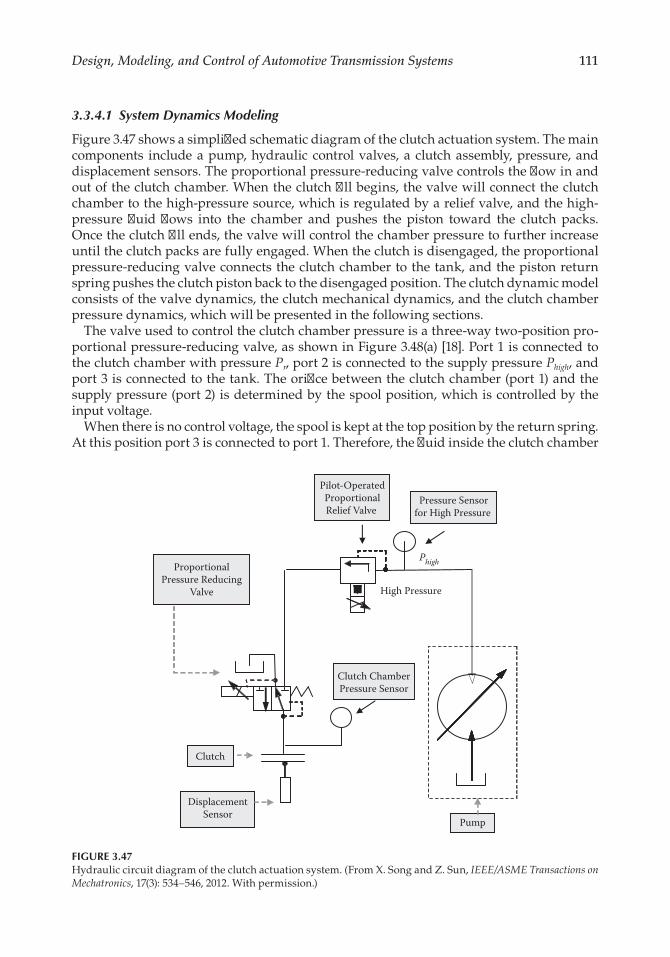
111Design, Modeling, and Control of Automotive Transmission Systems
3.3.4.1 System Dynamics Modeling
Figure 3.47 shows a simplified schematic diagram of the clutch actuation system. The main components include a pump, hydraulic control valves, a clutch assembly, pressure, and displacement sensors. The proportional pressure-reducing valve controls the flow in and out of the clutch chamber. When the clutch fill begins, the valve will connect the clutch chamber to the high-pressure source, which is regulated by a relief valve, and the high-pressure fluid flows into the chamber and pushes the piston toward the clutch packs. Once the clutch fill ends, the valve will control the chamber pressure to further increase until the clutch packs are fully engaged. When the clutch is disengaged, the proportional pressure-reducing valve connects the clutch chamber to the tank, and the piston return spring pushes the clutch piston back to the disengaged position. The clutch dynamic model consists of the valve dynamics, the clutch mechanical dynamics, and the clutch chamber pressure dynamics, which will be presented in the following sections.
The valve used to control the clutch chamber pressure is a three-way two-position pro-portional pressure-reducing valve, as shown in Figure 3.48(a) [18]. Port 1 is connected to the clutch chamber with pressure Pr, port 2 is connected to the supply pressure Phigh, and port 3 is connected to the tank. The orifice between the clutch chamber (port 1) and the supply pressure (port 2) is determined by the spool position, which is controlled by the input voltage.
When there is no control voltage, the spool is kept at the top position by the return spring. At this position port 3 is connected to port 1. Therefore, the fluid inside the clutch chamber
Pilot-OperatedProportionalRelief Valve
DisplacementSensor
Pump
ProportionalPressure Reducing
Valve
Clutch
High Pressure
Phigh
Pressure Sensorfor High Pressure
Clutch ChamberPressure Sensor
FIGURE 3.47Hydraulic circuit diagram of the clutch actuation system. (From X. Song and Z. Sun, IEEE/ASME Transactions on Mechatronics, 17(3): 534–546, 2012. With permission.)

112 Design and Control of Automotive Propulsion Systems
will flow to the tank. When a positive voltage is exerted on the magnetic coil, the induced magnetic force will push the spool toward port 1. As the spool connects port 1 to port 2, the high-pressure fluid will flow in to the clutch chamber. The increased pressure in port 1 will push the spool upward and eventually close the orifice between port 1 and port 2. Clearly, the spool position is determined by the magnetic force Fmag, the returning spring force Fspring, and the chamber pressure Pr. The spool dynamics can be described as [18]
=
= − +
− −
−
�
� 1( ) ( )
L v
vM
F Vol K L L
D v A P
spool spool
spoolspool
mag spring spool pre load
spool spool spool r
(3.39)
where
( ) = × = ×−
+F Vol K i Ki i
VolVol imag f f
max min
maxmin (3.40)
Lspool is the spool position, vspool is the spool velocity, Mspool is the spool mass, Kspring is the spool spring constant, Aspool is the cross-sectional area of the spool, and Dspool is the damp-ing coefficient. Lpreload is the spool position where the orifice between port 1 and port 2 is just closed. Fmag is the magnetic force, which is determined by the coil magnetic constant Kf
Lspool
dspool
Port 2
Port 1
Spool
ValveBody
(a) Spool at the tank port (b) Spool at the clutch chamber port
dspool
Port 3ValveBody
Return Spring
Spool
Seal
Port 1, to Clutch Chamber
Port 3, to Tank
Port 2, to HighPressure
Connection Pipe
Seal
Valve Body
θ
FIGURE 3.48Cross-sectional view of the proportional pressure-reducing valve. (From X. Song and Z. Sun, IEEE/ASME Transactions on Mechatronics, 17(3): 534–546, 2012. With permission.)
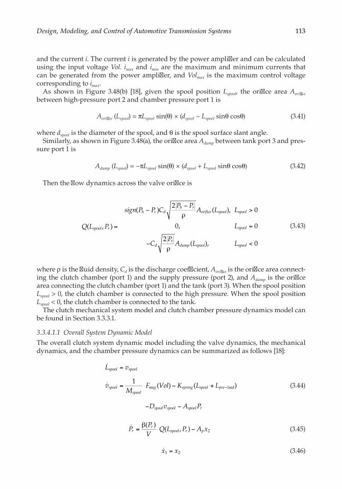
113Design, Modeling, and Control of Automotive Transmission Systems
and the current i. The current i is generated by the power amplifier and can be calculated using the input voltage Vol. imax and imin are the maximum and minimum currents that can be generated from the power amplifier, and Volmax is the maximum control voltage corresponding to imax.
As shown in Figure 3.48(b) [18], given the spool position Lspool, the orifice area Aorifice between high-pressure port 2 and chamber pressure port 1 is
Aorifice (Lspool) = πLspool sin(θ) × (dspool − Lspool sinθ cosθ) (3.41)
where dspool is the diameter of the spool, and θ is the spool surface slant angle.Similarly, as shown in Figure 3.48(a), the orifice area Adump between tank port 3 and pres-
sure port 1 is
Adump (Lspool) = −πLspool sin(θ) × (dspool + Lspool sinθ cosθ) (3.42)
Then the flow dynamics across the valve orifice is
( , )
( )2
( ), 0
0, 0
2( ), 0
=
−−ρ
>
=
−ρ
<
Q L P
sign P P CP P
A L L
L
CP
A L L
spool r
h r dh r
orifice spool spool
spool
dr
dump spool spool
(3.43)
where ρ is the fluid density, Cd is the discharge coefficient, Aorifice is the orifice area connect-ing the clutch chamber (port 1) and the supply pressure (port 2), and Adump is the orifice area connecting the clutch chamber (port 1) and the tank (port 3). When the spool position Lspool > 0, the clutch chamber is connected to the high pressure. When the spool position Lspool < 0, the clutch chamber is connected to the tank.
The clutch mechanical system model and clutch chamber pressure dynamics model can be found in Section 3.3.3.1.
3.3.4.1.1 Overall System Dynamic Model
The overall clutch system dynamic model including the valve dynamics, the mechanical dynamics, and the chamber pressure dynamics can be summarized as follows [18]:
1
( ) ( )
=
= − +
− −
−
�
�
L v
vM
F Vol K L L
D v A P
spool spool
spoolspool
mag spring spool pre load
spool spool spool r
(3.44)
( )
( , ) 2=β
−�PP
VQ L P A xr
rspool r p (3.45)
1 2x x=� (3.46)
114 Design and Control of Automotive Propulsion Systems
1( )
( , ) ( )
2 2
2 1 0
xM
A P P P D x
F P P x F x x
pp r c atm p
drag r c res p
= × × + − −
− + − +
� (3.47)
Fres is the displacement-dependent resistance force. During the clutch fill, the resistance force comes from the piston return spring; thus, the force Fres depends on the spring stiff-ness constant Kcs. During the clutch engagement, the resistance force is due to the squeez-ing of the clutch packs, and therefore the resistance force Fres can be modeled as
=× + ≤
+ >F
K x x x x
F x x x xrescs p fill
en p fill
( ) ( )
( ) ( )1 0 1
1 0 1 (3.48)
where the function Fen(x1 + xp0) includes both spring force and the nonlinear clutch pack reaction force; xfill is the clutch piston position at the end of the clutch fill.
Fdrag is the piston seal drag force, which is dependent on the piston motion.
( ) ( )
=+ + × ≠
=F
k P P c sign x x
F xdrag
m r c m
stick
( 0)
( 0)
2 2
2
(3.49)
where km and cm are constant, and Fstick is the static stick friction force from Kanopp’s stick-slip model [11]. Further detail of the mechanical dynamic model can be found in Section 3.3.3.1.
Further investigation reveals that the time constant of the pressure-reducing valve is far less than the time constant of the clutch actuation system pressure dynamics, which means that the dynamic behavior of the reducing valve can be neglected. Therefore, to simplify the control design, the proportional valve spool dynamics is converted into a static mapping;
1
( )= − × −−LK
F u K L A Pspoolspring
mag spring pre load spool r (3.50)
Here, we denote u = Vol as the control input to the proportional valve. Therefore, the sys-tem dynamics (Equations (3.44) and (3.45)) becomes
( )
( , ) 2=β
−�PP
VQ u P A xr
rr p (3.51)
where
( , )
( )2
( ), ( , ) 0
0, ( , ) 0
2( ), ( , ) 0
Q u P
sign P P CP P
A L L u P
L u P
CP
A L L u P
r
h r dh r
orifice spool spool r
spool r
dr
dump spool spool r
=
−−ρ
>
=
−ρ
<
(3.52)
Finally, the reduced order system dynamics includes Equations (3.46) to (3.52).
115Design, Modeling, and Control of Automotive Transmission Systems
In addition, for a given flow rate q, the required control input u can also be determined based on Equations (3.41), (3.42), (3.50), and (3.52). This relationship will be used in the next section, and the mapping from q to u can be written as
=−
×+ +
−−U q PVol
i iL K K L A P
Kir
max
max min
spool spring spring pre load spool r
fmin( , )
( ) (3.53)
where
4 cos( )
( )2
sin(2 ), 0
0, 0
4 cos( )
2
sin(2 ), 0
2
2
L
d dq
sign P P CP P
q
q
d dq
CP
q
spool
spool spool
h r dh r
spool spool
dr
=
− −θ
π −−ρ
θ>
=
− + +θ
πρ
θ<
(3.54)
Equation (3.54) is to calculate the spool position Lspool corresponding to a specific valve opening orifice based on Equations (3.41) and (3.42). The relationship between Equations (3.52) and (3.53) can be written as Q{U (q, Pr), Pr} = q.
3.3.4.2 Robust Nonlinear Controller and Observer Design
3.3.4.2.1 Sliding Mode Controller Design for Pressure Control
The clutch system (Equations (3.46) to (3.52)) is a third-order nonlinear system. As both the control input u (the valve voltage) and the control output Pr (the chamber pressure) appear in the dynamic equation (3.51), the system has a nonlinear dynamics with relative degree 1 [20]. Equations (3.46) and (3.47) are the system internal dynamics, the equilib-rium point of which is asymptotically stable. Therefore, the nonlinear system is minimum phase [20]. Note that the internal dynamics in this application is a spring mass damper system; therefore, the minimum phase feature also suggests that the whole system will be stabilized as long as the states other than the internal dynamics states could be stabilized. This unique feature suggests applying the sliding mode controller, which can ensure sys-tem robustness with a relatively low order controller design [20].
Define the tracking error e2 as the difference between the desired pressure trajectory r and the actual measurement Pr.
e2 = Pr − r (3.55)
And define another error term, e1, the derivative of which is equal to e2.
1 2e e=� (3.56)
116 Design and Control of Automotive Propulsion Systems
With the pressure dynamics in (3.51), we have
( )
( , ) ( , ) ( )
( )( , )
( )( )
( )( , )
2
2 2 1
2 1 2
= −
=β
+ − + −
=β
−β
− + +β
� � �
�
�
e P r
PV
Q u P u P A x P r
PV
Q u PP
VA x r P
PV
u P
r
rr r p r
rr
rp r
rr
(3.57)
where Δ1(Pr) represents the model uncertainty of the pressure dynamics (3.51), and Δ2(u, Pr) represents the model uncertainty of the pressure-reducing valve flow dynamics (3.52). Bounds of the uncertainty terms will be obtained experimentally in a later section.
Define the sliding surface S as
S = k1e1 + e2 (3.58)
where k1 is a weighting parameter.Then the controller can be designed as
�= −β
× −β
− −u UVP
k eP AV
x r v Pr
r pu r( )
( ),1 2 2 (3.59)
where U is defined in Equation (3.53); vu is a controller term to be designed later. As the piston velocity x2 cannot be measured directly due to the lack of a displacement and veloc-ity sensor, an observer is needed to estimate x1 and x2. The estimated states are not only fed back to the controller (3.59), but also used to evaluate the piston displacement, and therefore the clutch fill status. The observer design for piston motion will be presented in the next section. With the observed x2, the control input becomes
�
�
= −β
× −β
− −
= −β
× −β
× + − −
u UVP
k eP AV
x r v P
UVP
k eP AV
x x r v P
r
r pu r
r
r pu r
( )( ) ˆ ,
( )( )
( ( ˆ )) ,
1 2 2
1 2 2 3 2
(3.60)
where ˆ2x is the estimate of x2 and ( ˆ )3 2x is the estimation error.Then the sliding surface becomes
= +
= +
� � �
�
1 1 2
1 2 2
S k e e
k e e (3.61)
By substituting Equation (3.57) and Equation (3.60) into Equation (3.61), it becomes
( )
( , , ˆ )2SP
Vv u P xr
u r=β
+� (3.62)
where ( , , ˆ ) ( )( )
( , )( )
( ˆ )2 1 2 3 2u P x PP
Vu P
P AV
xr rr
rr p= +
β+β
.
117Design, Modeling, and Control of Automotive Transmission Systems
With Vlp = (1/2)S2 as the Lyapunov function for Equation (3.62), we have
= =β
+
≤β
+ ×
� � ( )
( )
V SSP
Vv S S
PV
v S S
lpr
u
ru
(3.63)
if
( )
( , ˆ )2 0V
PP x v
rr u
×β
≤ ψ + λ (3.64)
where ( , ˆ )2P xrψ is a positive continuous function, and λ0 is a real number in the (0,1) interval.Then vu can be designed as
( , ˆ ) ( )2v P x sign Su r= −γ (3.65)
where ( , ˆ )2P xrγ is the controller gain, and design γ ≥ψ
− λ+ γ γ >( , ˆ )
( , ˆ )1
, 022
00 0P x
P xr
r .
Substituting Equations (3.64) and (3.65) into Equation (3.63) gives [20]
( )
( )( , ˆ ) ( , ˆ ) ( , ˆ )
( )(1 )
0
2 2 0 2
0 0
≤β
+ ×
≤β
× −γ + ψ + λ γ
≤ −β
× γ × − λ
<
�VP
Vv S S
PV
P x P x P x S
PV
S
lpr
u
rr r r
r
which proves the convergence of the controller design.Finally, the controller is given as follows:
�= −β
× −β
× − + γu UVP
k eP AV
x r P x sign S Pr
r pr r( )
( ) ˆ ( , ˆ ) ( ),1 2 2 2 (3.66)
In the real-time implementation, to suppress the chattering problem, the sign function in (3.66) is approximated by a saturation function as [20]
( )sign S sat
S=
σ
where σ is a constant positive number. The control structure can therefore be summarized in Figure 3.49 [18].
As shown in Equation (3.66), implementation of the controller requires the uncertainty bound and the velocity estimation. A conservative uncertainty bound will make the controller gain γ too large, and thus result in chattering. Therefore, a proper estimation of the model uncertainty is critical. In addition, the piston velocity estimate ˆ2x is actu-ally a compensation term in the controller design (3.66), and it will influence the pressure tracking performance, especially during the clutch fill, where the piston velocity is higher. Besides, the clutch fill status can also be evaluated based on the piston motion estimate.

118 Design and Control of Automotive Propulsion Systems
Therefore, a piston motion observer is necessary and will be presented in the following section.
3.3.4.2.2 Observer Design
The observer is designed to estimate the clutch piston displacement x1 and velocity x2 using the pressure measurement Pr. During the clutch fill process, the piston velocity x2 is nonzero and the drag force Fdrag (Equation (3.49)) is only a function of the pressure. Also, the resistance force Fres (Equation (3.48)) is the piston return spring force, and thus is linear as well. Suppose y is the measurement of the chamber pressure Pr. The observer for the clutch fill process is designed as [18]:
ˆ ˆ( )
( , ) ˆ
ˆ 1( ) ˆ ( ) ( ˆ )
( )( , ) ˆ
1 2 1 2
2 2 1 0
2 2
x x LVy
y Q u y A x
xM
A y P P D x F y P K x x
LVy
y Q u y A x
p
pp c atm p drag c cs p
p
= + ×β
− +
= × + − − − + − × +
+ ×β
− +
� �
�
�
(3.67)
Suppose the estimation error is denoted as
ˆ
ˆ
1 1 1
2 2 2
x x
x x
ε = −
ε = − (3.68)
Combining Equations (3.67) and (3.46) to (3.51), we have
� �
�
ε = ε −β
− +
= ε − − +
= ε + ε
ε = − ε − ε + ε
LVy
y Q u y A x
L A x A x
L A
MD K L A
p
p p
p
pp cs p
( )( , ) ˆ
( ˆ )
1
1 2 1 2
2 1 2 2
2 1 2
2 2 1 2 2
(3.69)
Sliding ModeController
NonlinearObserver
PlantDynamics
u Chamber Pressure Output
Clutch Piston Displacement x1
Clutch FillDiagnosis
Ref Pressure
Piston Velocity x2
FIGURE 3.49Controller design structure. (From X. Song and Z. Sun, IEEE/ASME Transactions on Mechatronics, 17(3): 534–546, 2012. With permission.)
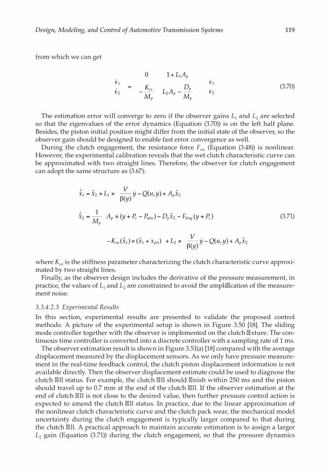
119Design, Modeling, and Control of Automotive Transmission Systems
from which we can get
��ε
ε=
+
− −
ε
ε
L A
KM
L ADM
p
cs
pp
p
p
0 11
2
1
2
1
2 (3.70)
The estimation error will converge to zero if the observer gains L1 and L2 are selected so that the eigenvalues of the error dynamics (Equation (3.70)) is on the left half plane. Besides, the piston initial position might differ from the initial state of the observer, so the observer gain should be designed to enable fast error convergence as well.
During the clutch engagement, the resistance force Fres (Equation (3.48)) is nonlinear. However, the experimental calibration reveals that the wet clutch characteristic curve can be approximated with two straight lines. Therefore, the observer for clutch engagement can adopt the same structure as (3.67):
ˆ ˆ( )
( , ) ˆ
ˆ 1( ) ˆ ( )
( ˆ ) ( ˆ )( )
( , ) ˆ
1 2 1 2
2 2
1 1 0 2 2
= + ×β
− +
= × + − − − +
− × + + ×β
− +
� �
�
�
x x LVy
y Q u y A x
xM
A y P P D x F y P
K x x x LVy
y Q u y A x
p
pp c atm p drag c
en p p
(3.71)
where Ken is the stiffness parameter characterizing the clutch characteristic curve approxi-mated by two straight lines.
Finally, as the observer design includes the derivative of the pressure measurement, in practice, the values of L1 and L2 are constrained to avoid the amplification of the measure-ment noise.
3.3.4.2.3 Experimental Results
In this section, experimental results are presented to validate the proposed control methods. A picture of the experimental setup is shown in Figure 3.50 [18]. The sliding mode controller together with the observer is implemented on the clutch fixture. The con-tinuous time controller is converted into a discrete controller with a sampling rate of 1 ms.
The observer estimation result is shown in Figure 3.51(a) [18] compared with the average displacement measured by the displacement sensors. As we only have pressure measure-ment in the real-time feedback control, the clutch piston displacement information is not available directly. Then the observer displacement estimate could be used to diagnose the clutch fill status. For example, the clutch fill should finish within 250 ms and the piston should travel up to 0.7 mm at the end of the clutch fill. If the observer estimation at the end of clutch fill is not close to the desired value, then further pressure control action is expected to amend the clutch fill status. In practice, due to the linear approximation of the nonlinear clutch characteristic curve and the clutch pack wear, the mechanical model uncertainty during the clutch engagement is typically larger compared to that during the clutch fill. A practical approach to maintain accurate estimation is to assign a larger L2 gain (Equation (3.71)) during the clutch engagement, so that the pressure dynamics

120 Design and Control of Automotive Propulsion Systems
can dominate in the observer estimation. The effect of the initial state of the observer is shown in Figure 3.51(b) [18]. Even with a 0.25 mm initial clutch position estimation error, the estimate converges to the actual value quickly. The effect of model uncertainties is investigated as well. Figure 3.52 [18] shows the estimation results when the piston return spring parameter Kp, the spring preload xp0, the clutch damping coefficient Dp, the piston
Flow Meter
PressureReducingValve
In ChamberPressureSensor
ClutchAssembly
Laser Sensor
InletPressureSensor
FIGURE 3.50The experimental setup for pressure-based clutch actuation. (Only pressure is used in the real-time feed-back, and other sensors are installed for dynamic modeling purposes.) (From X. Song and Z. Sun, IEEE/ASME Transactions on Mechatronics, 17(3): 534–546, 2012. With permission.)
0 0.05 0.1 0.15 0.2 0.25 0.3 0.35 0.4 0.45 0.50
0.5
1
Time (second)(a)
(b)
Pist
on D
ispla
cem
ent (
mm
)
Experimental displacementEstimated displacement
0 0.05 0.1 0.15 0.2 0.25 0.3 0.350
0.2
0.4
0.6
0.8
1
Time (second)
Pist
on D
ispla
cem
ent (
mm
)
Experimental displacementEstimated displacement
FIGURE 3.51The nonlinear observer estimation results. (a) Estimation with accurate initial state. (b) Estimation with inac-curate initial state. (From X. Song and Z. Sun, IEEE/ASME Transactions on Mechatronics, 17(3): 534–546, 2012. With permission.)
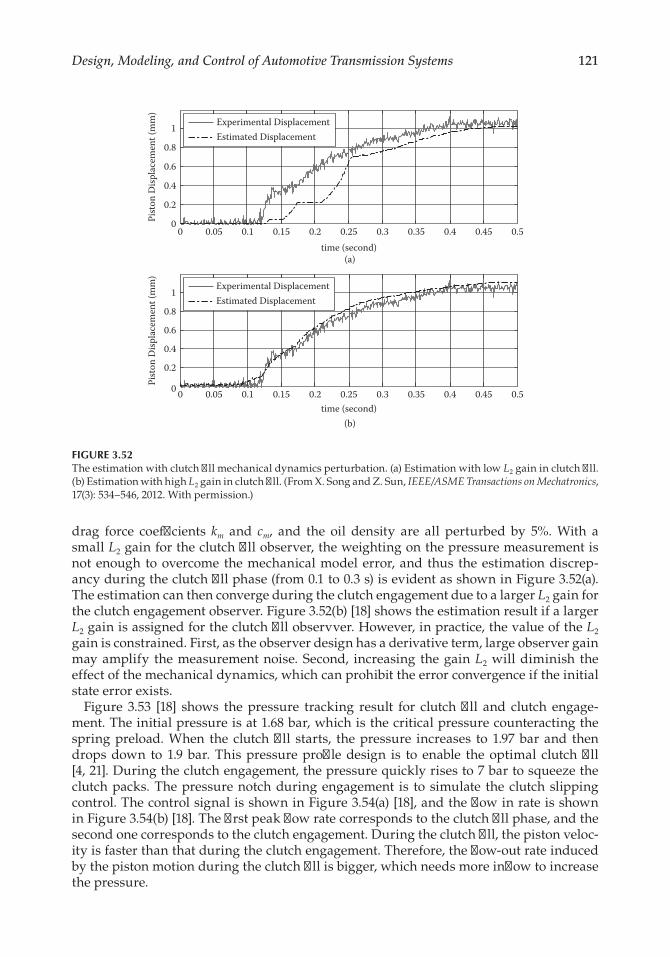
121Design, Modeling, and Control of Automotive Transmission Systems
drag force coefficients km and cm, and the oil density are all perturbed by 5%. With a small L2 gain for the clutch fill observer, the weighting on the pressure measurement is not enough to overcome the mechanical model error, and thus the estimation discrep-ancy during the clutch fill phase (from 0.1 to 0.3 s) is evident as shown in Figure 3.52(a). The estimation can then converge during the clutch engagement due to a larger L2 gain for the clutch engagement observer. Figure 3.52(b) [18] shows the estimation result if a larger L2 gain is assigned for the clutch fill observver. However, in practice, the value of the L2 gain is constrained. First, as the observer design has a derivative term, large observer gain may amplify the measurement noise. Second, increasing the gain L2 will diminish the effect of the mechanical dynamics, which can prohibit the error convergence if the initial state error exists.
Figure 3.53 [18] shows the pressure tracking result for clutch fill and clutch engage-ment. The initial pressure is at 1.68 bar, which is the critical pressure counteracting the spring preload. When the clutch fill starts, the pressure increases to 1.97 bar and then drops down to 1.9 bar. This pressure profile design is to enable the optimal clutch fill [4, 21]. During the clutch engagement, the pressure quickly rises to 7 bar to squeeze the clutch packs. The pressure notch during engagement is to simulate the clutch slipping control. The control signal is shown in Figure 3.54(a) [18], and the flow in rate is shown in Figure 3.54(b) [18]. The first peak flow rate corresponds to the clutch fill phase, and the second one corresponds to the clutch engagement. During the clutch fill, the piston veloc-ity is faster than that during the clutch engagement. Therefore, the flow-out rate induced by the piston motion during the clutch fill is bigger, which needs more inflow to increase the pressure.
0 0.05 0.1 0.15 0.2 0.25 0.3 0.35 0.4 0.45 0.50
0.2
0.4
0.6
0.8Pi
ston
Disp
lace
men
t (m
m)
time (second)(a)
1 Experimental DisplacementEstimated Displacement
(b)
0 0.05 0.1 0.15 0.2 0.25 0.3 0.35 0.4 0.45 0.50
0.2
0.4
0.6
0.8
1
time (second)
Pist
on D
ispla
cem
ent (
mm
)
Experimental DisplacementEstimated Displacement
FIGURE 3.52The estimation with clutch fill mechanical dynamics perturbation. (a) Estimation with low L2 gain in clutch fill. (b) Estimation with high L2 gain in clutch fill. (From X. Song and Z. Sun, IEEE/ASME Transactions on Mechatronics, 17(3): 534–546, 2012. With permission.)
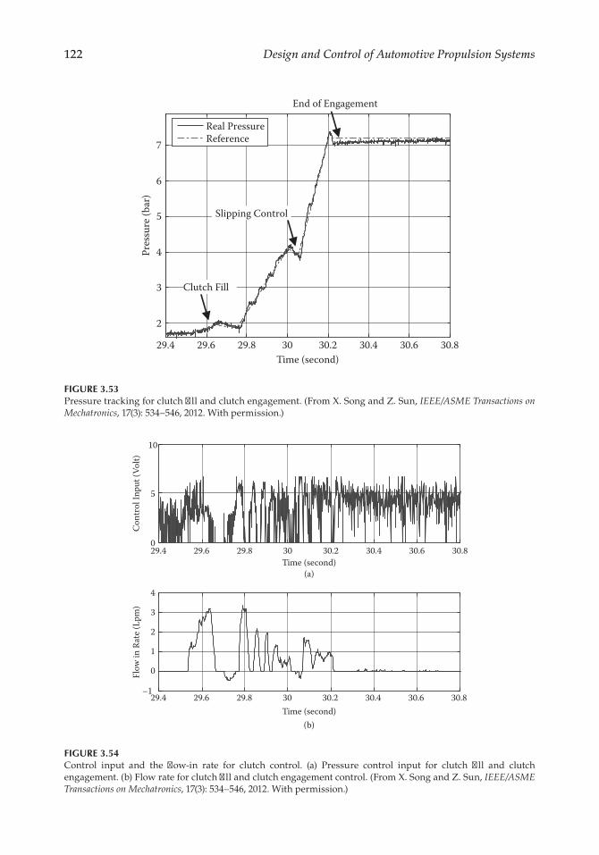
122 Design and Control of Automotive Propulsion Systems
29.4 29.6 29.8 30 30.2 30.4 30.6 30.8
2
3
4
5
6
7
Time (second)
Pres
sure
(bar
)
Real PressureReference
End of Engagement
Slipping Control
Clutch Fill
FIGURE 3.53Pressure tracking for clutch fill and clutch engagement. (From X. Song and Z. Sun, IEEE/ASME Transactions on Mechatronics, 17(3): 534–546, 2012. With permission.)
29.4 29.6 29.8 30 30.2 30.4 30.6 30.80
5
10
Time (second)(a)
Cont
rol I
nput
(Vol
t)
(b)
29.4 29.6 29.8 30 30.2 30.4 30.6 30.8–1
0
1
2
3
4
Time (second)
Flow
in R
ate (
Lpm
)
FIGURE 3.54Control input and the flow-in rate for clutch control. (a) Pressure control input for clutch fill and clutch engagement. (b) Flow rate for clutch fill and clutch engagement control. (From X. Song and Z. Sun, IEEE/ASME Transactions on Mechatronics, 17(3): 534–546, 2012. With permission.)
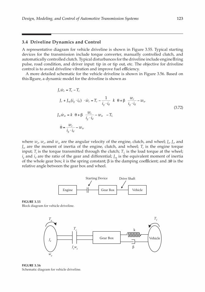
123Design, Modeling, and Control of Automotive Transmission Systems
3.4 Driveline Dynamics and Control
A representative diagram for vehicle driveline is shown in Figure 3.55. Typical starting devices for the transmission include torque converter, manually controlled clutch, and automatically controlled clutch. Typical disturbances for the driveline include engine firing pulse, road condition, and driver input: tip in or tip out, etc. The objective for driveline control is to avoid driveline vibration and improve fuel efficiency.
A more detailed schematic for the vehicle driveline is shown in Figure 3.56. Based on this figure, a dynamic model for the driveline is shown as
( )1
J w T T
J J i i w Ti i
kw
i iw
J w kw
i iw T
wi i
w
e e e c
c eq g d c cg d
c
g dw
w wc
g dw L
c
g dw
= −
+ ⋅ ⋅ = −⋅
θ + β⋅
−
= θ + β⋅
− −
θ =⋅
−
�
�
�
�
(3.72)
where we, wc, and ww are the angular velocity of the engine, clutch, and wheel; Je, Jc, and Jw are the moment of inertia of the engine, clutch, and wheel; Te is the engine torque input; Tc is the torque transmitted through the clutch; TL is the load torque at the wheel; ig and id are the ratio of the gear and differential; Jeq is the equivalent moment of inertia of the whole gear box; k is the spring constant; β is the damping coefficient; and Δθ is the relative angle between the gear box and wheel.
Engine Gear Box Vehicle
Starting Device Drive Shaft
FIGURE 3.55Block diagram for vehicle driveline.
Gear Box Vehicle
Te
Je
we
Tc
Jcwc
k
β
Tl
FIGURE 3.56Schematic diagram for vehicle driveline.

124 Design and Control of Automotive Propulsion Systems
When the clutch is engaged, that is, we = wc, we have
J J J i i w Ti i
kw
i iw
J w kw
i iw T
wi i
w
e c eq g d c eg d
c
g dw
w wc
g dw L
c
g dw
+ + ⋅ = −⋅
θ + β⋅
−
= θ + β⋅
− −
θ =⋅
−
�
�
�
( )1
Since we = wc, the system becomes third order. From the dynamic models, we can see that the clutch torque Tc is critical for system performance and fuel economy. If Tc is not controlled properly, we could have engine flare, engine misfire, driveline vibration, and sluggish gear shift.
Let’s further examine the controllability of the system. First let’s further simplify the system dynamics: assume Δθ = 0; i.e., the driveshaft is a solid connection. We then have
J w T T
J w T T
e e e c
v c c l
= −
= −
�
�
Let x1 = θe , x2 = we, x3 = θc , x4 = wc; we have
x x
xJ
T T
x x
xJ
T T
xxxx
xxxx
JT T
JT T
ee c
vc l
ee c
vc l
=
= −
=
= −
= +−
−
�
�
�
�
����
1[ ]
1[ ]
0 1 0 00 0 0 00 0 0 10 0 0 0
01
[ ]
01
[ ]
1 2
2
3 4
4
1
2
3
4
1
2
3
4
If the only control variable is Tc, we have
= =
−
A BJ
J
e
v
0 1 0 00 0 0 00 0 0 10 0 0 0
,
01
01

125Design, Modeling, and Control of Automotive Transmission Systems
And the controllability matrix is
−
−
J
J
J
J
e
e
v
v
0 01
0
0 0 01
0 01
0
0 0 01
which is not full rank.This suggests that by controlling the clutch torque only, we cannot control the engine
speed and the vehicle speed independently. However, if we have two control variables, Tc and Te, we then have
A BJ J
J
e e
v
= =−0 1 0 0
0 0 0 00 0 0 10 0 0 0
,
0 01 1
0 01
0
The controllability matrix is then
−
−
J J
J J
J
J
e e
e e
v
v
0 0 0 01 1
0 0
0 0 0 0 0 01 1
0 0 0 01
0 0 0
0 0 0 0 0 01
0
which is full rank.This suggests that to have complete control over the engine and vehicle speed, two
control inputs, the engine torque and the clutch torque, are required. However, the engine torque is often controlled by the drive through the throttle. The clutch torque, however, can be fully controlled by the driveline controller. So it would be interesting to understand the exact impact of the clutch torque.
Define x5 = x1 – x3, x6 = x2 – x4. By considering the clutch slip speed as the state variable, and using Tc as the only control, we have
0 10 0
01 1 1 15
6
5
6= + + − +
��xx
xx
JT
JT
J JT
ee
vl
e vc
126 Design and Control of Automotive Propulsion Systems
So
= =− +
A BJ Je v
0 10 0
,
0
1 1
The controllability matrix is
− +
− +
J J
J J
e e
e e
1 10
01 1
which is full rank.This suggests that the clutch torque can have complete control over the slip speed.
This is important when designing clutch control to achieve the desired driveline objective.When simulating driveline dynamics, various driving cycles are often used, such as
the Federal Testing Procedure (FTP) used by the Environmental Protection Agency (EPA). Given a specific driving cycle, the vehicle power demand can be calculated using the method presented in Chapter 1. The engine operating point and the transmission gear ratio can also be calculated. This will allow the systematic evaluation of different driveline control methodologies in a realistic driving scenario.
References
1. X. Song, A. Mohd Zulkefli, Z. Sun, and H. Miao, Automotive Transmission Clutch Fill Control Using a Customized Dynamic Programming Method, Journal of Dynamic Systems, Measurement, and Control, 133: 054503, 2011.
2. Z. Sun and H. Kumar, Challenges and Opportunities in Automotive Transmission Control, presented at Proceedings of American Control Conference, Portland, OR, June 8–10, 2005.
3. X. Song, C. Wu, and Z. Sun, Design, Modeling, and Control of a Novel Automotive Transmission Clutch Actuation System, IEEE/ASME Transactions on Mechatronics, 17(3): 582–587, 2012.
4. H. Miao, Z. Sun, J. Fair, J. Lehrmann, and S. Harbin, Modeling and Analysis of the Hydraulic System for Oil Budget in an Automotive Transmission, presented at Proceedings of ASME Dynamic Systems and Control Conference, Ann Arbor, MI, October 20–22, 2008.
5. M. Montanari, F. Ronchi, C. Rossi, A. Tilli, and A. Tonielli, Control and Performance Evaluation of a Clutch Servo System with Hydraulic Actuation, Journal of Control Engineering Practice, 12(11): 1369–1379, 2004.
6. J. Horn, J. Bamberger, P. Michau, and S. Pindl, Flatness-Based Clutch Control for Automated Manual Transmissions, Journal of Control Engineering Practice, 11(12): 1353–1359, 2003.
7. L. Glielmo, L. Iannelli, and V. Vacca, Gearshift Control for Automated Manual Transmissions, IEEE/ASME Transactions on Mechatronics, 11(1): 17–26, 2006.
8. R.E. Bellman, Dynamic Programming, Princeton, NJ: Princeton University Press, 1957. 9. R.E. Bellman and S.E. Dreyfus, Applied Dynamic Programming, Princeton, NJ: Princeton
University Press, 1962.
127Design, Modeling, and Control of Automotive Transmission Systems
10. A.P. De Madrid, S. Dormido, and F. Morilla, Reduction of the Dimensionality of Dynamic Programming: A Case Study, in Proceedings of American Control Conference, San Diego, CA, June 1999, pp. 2852–2856.
11. D. Karnopp, Computer Simulation of Stick-Slip Friction in Mechanical Dynamic Systems, Journal of Dynamic Systems, Measurement, and Control, 107(1): 100–103, 1985.
12. X. Song, A. Zulkefli, Z. Sun, and H. Miao, Modeling, Analysis, and Optimal Design of the Automotive Transmission Ball Capsule System, Journal of Dynamic Systems, Measurement, and Control, 132: 021003, 2010.
13. X. Song, Z. Sun, X. Yang, and G. Zhu, Modeling, Control and Hardware-in-the-Loop Simulation of an Automated Manual Transmission, Journal of Automobile Engineering, 224(2): 143–160, 2010.
14. E. Hairer and G. Wanner, Solving Ordinary Differential Equations II, 2nd ed., Springer Series in Computational Mathematics, Berlin: Springer, 1996.
15. W. Gautschi, Numerical Analysis: An Introduction, Boston: Birkhauser, 1997. 16. J.M. Kang, I. Kolmanovsky, and J.W. Grizzle, Dynamic Optimization of Lean Burn Engine
Aftertreatment, Journal of Dynamic Systems, Measurement, and Control, 123(2): 153–160, 2001. 17. J.L. Crassidis and J.L. Junkins, Optimal Estimation of Dynamic Systems, CRC Applied Mathematics
and Nonlinear Science Series, Boca Raton, FL: Chapman and Hall/CRC Express LLC, 2004. 18. X. Song and Z. Sun, Pressure Based Clutch Control for Automotive Transmissions Using a
Sliding Mode Controller, IEEE/ASME Transactions on Mechatronics, 17(3): 534–546, 2012. 19. F. Vasca, L. Iannelli, A. Senatore, and G. Reale, Torque Transmissibility Assessment for
Automotive Dry-Clutch Engagement, IEEE/ASME Transactions on Mechatronics, 16(3): 564–573, 2011.
20. H. Khalil, Nonlinear Systems, 3rd ed., Upper Saddle River, NJ: Prentice Hall, 2002. 21. X. Song, A. Mohd Zulkefli, and Z. Sun, Automotive Transmission Clutch Fill Optimal Control:
An Experimental Investigation, presented at Proceedings of American Control Conference, Baltimore, MD, June 30–July 2, 2010.

129
4Design, Modeling, and Control of Hybrid Systems
4.1 Introduction to Hybrid Vehicles
As shown in Chapter 1, the fundamental challenge that limits powertrain efficiency is the varying vehicle speed and power demand in real time and the dependence of engine effi-ciency on speed and load conditions. Powertrain hybridization is one of the most effective ways for addressing this challenge. As the name suggests, a hybrid powertrain consists of the conventional internal combustion engine (ICE) and an alternative power source. Therefore, a hybrid transmission is needed to combine the power from the ICE and the alternative power source and send it to the wheels of the vehicle. Depending on the type of alternative power source and the architecture of the hybrid transmission, hybrid vehicles can be divided into different categories. Detailed discussions on the types of hybrid vehi-cles and the hybrid architectures will be provided in Sections 4.1.1 and 4.2.
The basic fuel-saving mechanisms for hybrid vehicles include: (1) optimize the engine operating condition independent from the vehicle operating condition using the extra degree of freedom enabled by the alternative power source, (2) use an energy storage ele-ment to provide a buffer between the engine power generation and the vehicle power demand, and (3) provide regenerative braking by converting the vehicle kinetic energy during braking into energy storage for future use. For the first fuel-saving mechanism, a large energy storage element is not necessary. However, for the second and third fuel-saving mechanisms, an energy or power storage element is essential to achieve the desired functions, which has been a key technical challenge for hybrid vehicle development.
The research and development of hybrid vehicles has been mainly focused on the design of the hybrid architecture [1] and the energy management of the hybrid powertrain [2, 3]. In this chapter, we will first present different types of hybrid vehicles, and then discuss the hybrid architecture design, and finally show the hybrid powertrain dynamics and control.
4.1.1 Various Types of Hybrid Vehicles
So far several different types of hybrid vehicles have been proposed: hybrid electric vehi-cle (HEV), hydraulic hybrid vehicle, pneumatic hybrid vehicle, and hybrid mechanical vehicle. As the names suggest, the main difference among the various hybrid vehicles is the type of alternative power source employed.
The hybrid electric vehicle complements the ICE with the electrical motor/generator and uses a battery to store the energy. The hydraulic hybrid vehicle uses the hydraulic accumulator to store energy or power and the hydraulic pump/motor as the actuation device. The pneumatic hybrid vehicle uses a compressed air tank to store energy and the pneumatic pump/motor to transmit power. The hybrid mechanical vehicle stores energy

130 Design and Control of Automotive Propulsion Systems
with a mechanical fly wheel and the mechanical energy can be transmitted with clutches and other mechanisms, such as gears.
Each type of hybrid vehicle has its advantages and disadvantages. The main properties for differentiating the hybrid vehicles include energy density, power density, cost, reli-ability, and ease for control. So far, the hybrid electric vehicle has the largest market share and is mainly focused on passenger cars. The hydraulic hybrid vehicle has been the main hybrid technology for heavy vehicles. As will be shown in Section 4.2, the hybrid architec-ture is applicable to different hybrid vehicles even though the underlying physical systems are different. A similar statement can be made for hybrid powertrain dynamics and con-trol, which will be presented in Section 4.3.
4.2 Hybrid Architecture Analysis
4.2.1 Parallel Hybrid Architecture
As shown in Figure 4.1, the parallel architecture employs an alternative power unit (APU) in parallel with the ICE. The APU can either assist the torque output from the engine or load the engine. This will allow the engine to operate at loading conditions that are different from the vehicle power demand (see Chapter 1) to optimize its efficiency and emissions. However, with the parallel architecture, the speed of the ICE cannot be inde-pendently varied from the vehicle speed since it is still constrained by the transmission (see Chapter 3). This will greatly limit the flexibility of the parallel architecture. Besides changing the loading conditions of the engine, the parallel architecture can also enable the stop-and-go function and provide limited regenerative braking. The stop-and-go function is realized by shutting down the engine when the vehicle comes to a full stop and restart-ing the engine using the APU when the vehicle is ready to launch again. This function will help to reduce the engine idling time and save fuel. The regenerative braking can be achieved by converting the vehicle kinetic energy into the alternative energy (such as electricity) through the APU (such as a generator). But this function is often limited by the size of the APU and the energy storage device, as well as safety considerations of the brak-ing operation. Of course, regenerative braking is also dependent on the amount of kinetic energy available when braking is initiated. This can vary drastically depending on the size
ICE Transmission
APU
Vehicle
Propulsion System
FIGURE 4.1Diagram of parallel hybrid architecture.
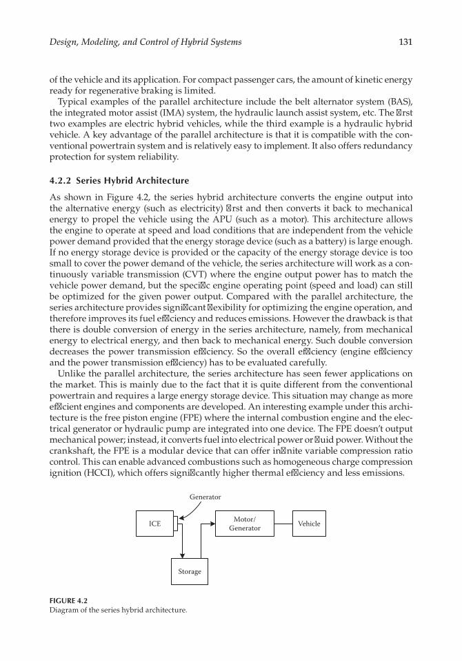
131Design, Modeling, and Control of Hybrid Systems
of the vehicle and its application. For compact passenger cars, the amount of kinetic energy ready for regenerative braking is limited.
Typical examples of the parallel architecture include the belt alternator system (BAS), the integrated motor assist (IMA) system, the hydraulic launch assist system, etc. The first two examples are electric hybrid vehicles, while the third example is a hydraulic hybrid vehicle. A key advantage of the parallel architecture is that it is compatible with the con-ventional powertrain system and is relatively easy to implement. It also offers redundancy protection for system reliability.
4.2.2 Series Hybrid Architecture
As shown in Figure 4.2, the series hybrid architecture converts the engine output into the alternative energy (such as electricity) first and then converts it back to mechanical energy to propel the vehicle using the APU (such as a motor). This architecture allows the engine to operate at speed and load conditions that are independent from the vehicle power demand provided that the energy storage device (such as a battery) is large enough. If no energy storage device is provided or the capacity of the energy storage device is too small to cover the power demand of the vehicle, the series architecture will work as a con-tinuously variable transmission (CVT) where the engine output power has to match the vehicle power demand, but the specific engine operating point (speed and load) can still be optimized for the given power output. Compared with the parallel architecture, the series architecture provides significant flexibility for optimizing the engine operation, and therefore improves its fuel efficiency and reduces emissions. However the drawback is that there is double conversion of energy in the series architecture, namely, from mechanical energy to electrical energy, and then back to mechanical energy. Such double conversion decreases the power transmission efficiency. So the overall efficiency (engine efficiency and the power transmission efficiency) has to be evaluated carefully.
Unlike the parallel architecture, the series architecture has seen fewer applications on the market. This is mainly due to the fact that it is quite different from the conventional powertrain and requires a large energy storage device. This situation may change as more efficient engines and components are developed. An interesting example under this archi-tecture is the free piston engine (FPE) where the internal combustion engine and the elec-trical generator or hydraulic pump are integrated into one device. The FPE doesn’t output mechanical power; instead, it converts fuel into electrical power or fluid power. Without the crankshaft, the FPE is a modular device that can offer infinite variable compression ratio control. This can enable advanced combustions such as homogeneous charge compression ignition (HCCI), which offers significantly higher thermal efficiency and less emissions.
ICE Motor/Generator
Storage
Vehicle
Generator
FIGURE 4.2Diagram of the series hybrid architecture.

132 Design and Control of Automotive Propulsion Systems
4.2.3 Power-Split Hybrid Architecture
As shown in Figure 4.3, the power-split architecture employs a hybrid transmission to combine the power from the ICE and the motor/generator sets and transmit it to the vehicle. The hybrid transmission often consists of one or several planetary gear sets. A key property of the planetary gear set is that for the speeds at the three nodes (sun, carrier, and ring), only after two speeds are determined can the third speed be decided (for details see Chapter 3). This is essentially a two degrees of freedom system, which enables the flexibility of varying engine operating conditions (speed and torque) by controlling the motor/generator set. The power-split architecture combines the benefits of the parallel and series architecture by splitting the engine power into the mechanical and the electrical path. Specifically, the mechanical path refers to the power flowing through the planetary gear sets and transmitting to the vehicle mechanically. The electrical path refers to the power that is converted from mechanical power into electrical power through a generator, and eventually converted back to mechanical power through a motor. This architecture enables the engine to vary its operating condition independent of the vehicle operating condition, while still transmitting part of its power through the mechanical path to avoid double conversion of energy. This architecture offers a good compromise between flexibil-ity and power transmission efficiency.
There are several vehicles on the market that employ the power-split architecture. One example is the THS system, as shown in Figure 4.4. The engine is connected to the carrier, and the generator is connected to the sun gear. Ring gear is connected to the output. The motor is coupled to the output shaft. For any given vehicle speed, the engine speed can be
HybridTransmission
(PlanetaryGear Set)
ICE
Motor/Generator Set
Vehicle
FIGURE 4.3Diagram of the power-split architecture.
R
C
S
Motor
Engine
Generator
Di�erential
Vehicle
Countershaft Gears
PlanetaryGear Set
FIGURE 4.4Diagram of the THS system.
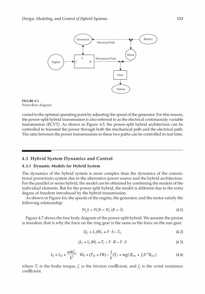
133Design, Modeling, and Control of Hybrid Systems
varied to the optimal operating point by adjusting the speed of the generator. For this reason, the power-split hybrid transmission is also referred to as the electrical continuously variable transmission (ECVT). As shown in Figure 4.5, the power-split hybrid architecture can be controlled to transmit the power through both the mechanical path and the electrical path. The ratio between the power transmissions in these two paths can be controlled in real time.
4.3 Hybrid System Dynamics and Control
4.3.1 Dynamic Models for Hybrid System
The dynamics of the hybrid system is more complex than the dynamics of the conven-tional powertrain system due to the alternative power source and the hybrid architecture. For the parallel or series hybrid, the model can be obtained by combining the models of the individual elements. But for the power-split hybrid, the model is different due to the extra degree of freedom introduced by the hybrid transmission.
As shown in Figure 4.6, the speeds of the engine, the generator, and the motor satisfy the following relationship:
WgS + WrR = We (R + S) (4.1)
Figure 4.7 shows the free body diagram of the power-split hybrid. We assume the pinion is massless; that is why the force on the ring gear is the same as the force on the sun gear.
I I W F S TG S G G( )+ = ⋅ −� (4.2)
I I W T F R F SE C e e( )+ = − ⋅ − ⋅� (4.3)
I ImR
kW T FR
kT mgf R f V RR M
tireR M f r tire d tire( )
1( )
2
22+ + = + − + +� (4.4)
where Tf is the brake torque, fr is the friction coefficient, and fd is the wind resistance coefficient.
Engine
Motor
Generator
Gear
SC R
Battery
Vehicle
Electrical Path
Mechanical Path
FIGURE 4.5Power flow diagram.

134 Design and Control of Automotive Propulsion Systems
From (4.1), we can get W S W R W R SG R e ( )+ = +� � � .The state of the charge for the battery can be modeled as
SOCI
Qbatt
max= −� (4.5)
where Qmax is the battery capacity and Ibatt is the current drawing from the battery.The battery power is
P V I I Rbatt oc batt batt batt2= − (4.6)
where VOC is the battery open-circuit voltage and Rbatt is the battery internal resistance.Since the battery power is either used to drive the motor or charged through the
generator, we also have
P T W T Wbatt G G GK
iK
M M MK
iK( )1 2= η η + η η (4.7)
S
C
R
G
M
E
FIGURE 4.6Block diagram of the power-split hybrid architecture.
FS
C
Rm k IM
Vehicle Mass
Vehicle Resistance
FR
FR+FS
IG TG
IE
Te
TM
FIGURE 4.7Free body diagram of the power-split architecture.

135Design, Modeling, and Control of Hybrid Systems
where ηG is the efficiency of the generator, ηM is the efficiency of the motor, ηi1 is the efficiency of inverter 1, ηi2 is the efficiency of inverter 2, K = 1 is the charging (power goes to the battery), and K = –1 is the discharging (power comes out of the battery).
From (4.5) to (4.7), we get
SOCV V T W T W R
R QOC OC G G G
KiK
M M MK
iK
batt
batt
4( )2
21 2
max= −
− − η η + η η� (4.8)
This model can be further extended by including the driveline dynamics, motor/ generator, and power electronics dynamics.
The dynamic model of the permanent magnet (PM) AC synchronous machine is
L I V R I L W I
L I V R I L W I W
T n I L L I I
d d d S d P q m q
q q q S q P d m d m P m
M P m q d q d q32
[ ( ) ]
= − + η
= − − η − ψ η
= ψ + −
�
� (4.9)
where Vd, Vq are the direct and quadrature axis voltages, Id, Iq are the direct and quadrature axis currents, Ld, Lq are the direct and quadrature axis inductances, Wm is the motor speed, TM is the motor torque, RS is the series phase resistance, nP is the number of pole pairs, and ψm is the permanent magnet flux.
4.3.2 Hybrid System Control
The majority of the published work on hybrid system control is focused on energy manage-ment [4–12]. In this section we will discuss two energy management strategies (Sections 4.3.2.1 and 4.3.2.2) and the driveline dynamics control of the hybrid system (Section 4.3.2.3).
4.3.2.1 Transient Emission and Fuel Efficiency Optimal Control
Both gasoline engines and diesel engines can be used for the hybrid application. The die-sel HEV is expected to offer even more fuel savings given the high efficiency of the diesel engine. However, the diesel HEV has an inherent disadvantage of high NOx and soot emissions, especially under transient operations [13, 14]. Targeted at achieving both the global energy optimization and transient emissions control, a two-mode hybrid pow-ertrain energy management strategy is designed [15]. First, dynamic programming (DP) is employed to ensure the global fuel efficiency optimization and battery state of charge (SOC) sustainability for any given driving cycles. On this basis, during selected emissions-reducing modes, the management strategy locally modifies the engine operations into another trajectory with the purpose of reducing the high transient emissions, and more importantly, at the end of every emissions-reducing mode, the locally optimized engine operating trajectory will be driven back to match the globally optimized trajectory gener-ated by the DP for the succeeding operation. This design ensures the global optimization of the fuel efficiency (albeit with some slight deviations in some areas) and battery SOC sustainability since the DP-optimized engine/battery operations are recovered after every local emission optimization. Specifically, in the fuel efficiency-improving mode, the man-agement strategy makes use of the DP algorithm to seek the global optimization of the fuel

136 Design and Control of Automotive Propulsion Systems
efficiency over the entire driving cycle; while in the emission-reducing mode, this strategy utilizes a linear quadratic regulator (LQR) to locally optimize the operating trajectory in a short time horizon, to suppress the surging emissions due to the sudden engine torque transients. Here, it is worth noting that we avoid directly adding the transient emis-sion optimization task into the DP global optimization algorithm, which will otherwise significantly increase the computational burden of DP.
4.3.2.1.1 Control-Oriented Emission Model
Targeted at realizing simultaneous fuel consumption and emission control, both the engine fuel consumption and emission models are needed. Different from the static mapping-based fuel consumption model, the emission model must involve higher-order transient dynam-ics. Ideally, to precisely describe the complex thermodynamics and chemistry of the engine combustion, the complete engine transient emissions model should contain as many high-fidelity physics-based submodels as possible that can catch the various engine processes (in-cylinder processes, inlet/exhaust manifold operation, exhaust gas recirculation (EGR) operation, turbocharger operation, and so on) and identify the effects of all the key operating parameters (engine speed, fuel injection mass, inlet air pressure, exhaust gas temperature, EGR opening, and so on). However, to implement the transient emission control in real time, a simplified, control-oriented model with well-selected input variables is required.
Various control-oriented emission models have been reported. A dynamic model com-posed of steady-state emission and transient emission correction was adopted in [16], where some process variables that represent the engine combustion or cylinder charge characteristics are used as inputs to characterize the transient emission effects. Otherwise, actual EGR opening rate, fresh air mass flow, and fuel/air ratio are also commonly used for transient correction [17, 18]. However, the previous emission models are commonly used for improving the engine operation within the engine control unit (ECU), but not for the vehicle-level energy management strategy. Recently, some studies on the emission models that are suitable for the vehicle-level control are also reported. In [19], a Volterra series-based model with fuel flow rate and engine speed as the inputs is presented.
Aiming at developing a hybrid vehicle energy management strategy that can optimize the fuel consumption over the entire driving cycle and reduce local transient emissions, a data-driven emission model that is capable of predicting the transient emission is built and identified by experiments. The modeling and validation process consists of two steps:
1. Input parameters selection. Although empirical data have shown that the engine internal variables (inlet air pressure, exhaust gas temperature, EGR opening, etc.) are closely coupled with both NOx and soot emissions, including those variables will increase the dimension of the emission model and, consequently, the compu-tational burden of the vehicle-level energy management. Therefore, the proposed model chooses the engine external variables (driver’s control inputs)—engine speed ωe and engine torque Te—as the inputs. Such selection is based on the obser-vation that the other key variables (such as the inlet air pressure, exhaust tempera-ture, and so on) are ultimately determined by the current engine speed and torque command (or their derivatives).
As a result, this input parameters selection brings us two advantages. First, the engine torque and speed are more accessible than the engine internal variables (i.e., ECU control actions), and second, these control inputs can directly deter-mine the engine fuel consumption in the static mapping model, which is advan-tageous for coordinating the optimal controls of both the fuel consumption and
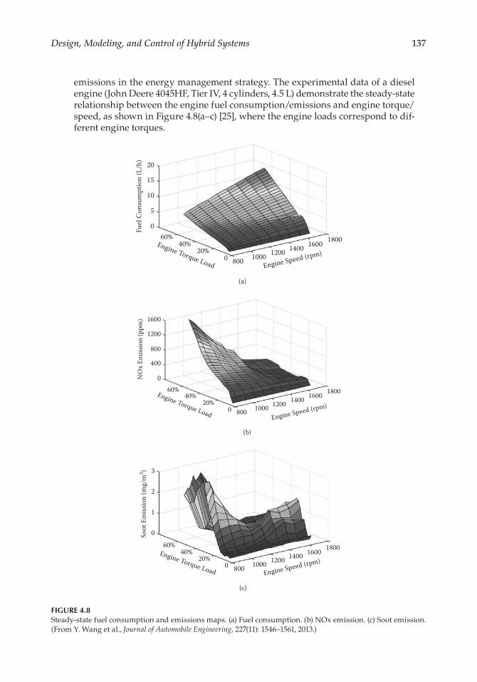
137Design, Modeling, and Control of Hybrid Systems
emissions in the energy management strategy. The experimental data of a diesel engine (John Deere 4045HF, Tier IV, 4 cylinders, 4.5 L) demonstrate the steady-state relationship between the engine fuel consumption/emissions and engine torque/speed, as shown in Figure 4.8(a–c) [25], where the engine loads correspond to dif-ferent engine torques.
20
Fuel
Con
sum
ptio
n (L
/h)
15
10
5
060%
40%20%
0
(a)
800 1000 1200
Engine Speed (rpm)Engine Torque Load
1400 1600 1800
1600
1200
800
400
060%
40%20%
0 800 1000 1200 1400 1600 1800
NO
x Em
issio
n (p
pm)
Engine Speed (rpm)Engine Torque Load
(b)
3
Soot
Em
issio
n (m
g/m
3 )
2
1
060%
40%20%
0 800 1000 1200
Engine Speed (rpm)Engine Torque Load
1400 1600 1800
(c)
FIGURE 4.8Steady-state fuel consumption and emissions maps. (a) Fuel consumption. (b) NOx emission. (c) Soot emission. (From Y. Wang et al., Journal of Automobile Engineering, 227(11): 1546–1561, 2013.)

138 Design and Control of Automotive Propulsion Systems
In addition, to capture the transient emission dynamics without introducing new independent variables, the derivatives of engine speed eω� and engine torque Te� are used as additional inputs. The physical explanation of eω� and Te
� as additional inputs to capture the transient emission dynamics is illustrated in Figures 4.9 and 4.10 [25]. Under different engine load transient conditions (different torque deriva-tives), the fuel injection flow rate will present different transients, which in turn affects the transient air/fuel ratio, and hence the emission output. The faster the engine load changes, i.e., the larger the torque derivative Te
� , the higher the transient fuel flow rate becomes, as shown in Figure 4.9. However, the inlet airflow rate is limited by the air pressure dynamics. Eventually, the transient air/fuel ratio that can directly cause undesired emission output is coupled with the torque deriva-tive Te
� , as shown in Figure 4.10. 2. Control-oriented model development and validation. With the well-selected input
variables, a proper mathematic model should be constructed to describe the nonlin-ear emission dynamics with relatively compact structure. To capture the nonlinear
50%
40%
30%
20%
10%
00 5 10 15
Time (s)
(a)
Engi
ne T
orqu
e Loa
d
Fuel
Flo
w (L
/h)
Fuel flowEngine torque load
20 25 30 350
2
4
6
8
10
12
50%
40%
30%
20%
10%
00 5 10 15
Time (s)
Engi
ne T
orqu
e Loa
d
Fuel
Flo
w (L
/h)
Fuel flowEngine torque load
20 25 30 350
2
4
6
8
10
12
(b)
FIGURE 4.9Engine fuel injections under different torque transients. (a) Torque rise time, 5 s. (b) Torque rise time, 1 s.
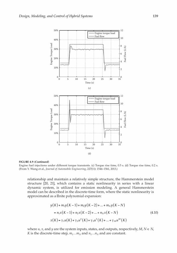
139Design, Modeling, and Control of Hybrid Systems
relationship and maintain a relatively simple structure, the Hammerstein model structure [20, 21], which contains a static nonlinearity in series with a linear dynamic system, is utilized for emission modeling. A general Hammerstein model can be described in the discrete-time form, where the static nonlinearity is approximated as a finite polynomial expansion:
( ) ( ) ( ) ( )
( ) ( ) ( )
( ) ( ) ( ) ( ) ( )
+ − + − + + −
= − + − + + −
= γ + γ + γ + + γ
1 2 ...
1 2 ...
...
1 2
1 2
1 22
33
y K m y K m y K m y K N
n x K n x K n x K N
x K u K u K u K u K
N
N
MM
(4.10)
where u, x, and y are the system inputs, states, and outputs, respectively, M, N ∈ N, K is the discrete-time step, m1…mN and n1…nN and are constant.
50%
40%
30%
20%
10%
00 5 10 15
Time (s)
Engi
ne T
orqu
e Loa
d
Fuel
Flo
w (L
/h)
Fuel flowEngine torque load
20 25 30 350
2
4
6
8
10
12
(c)
50%
40%
30%
20%
10%
00 5 10 15
Time (s)
Engi
ne T
orqu
e Loa
d
Fuel
Flo
w (L
/h)
Fuel flowEngine torque load
20 25 30 350
2
4
6
8
10
12
(d)
FIGURE 4.9 (Continued)Engine fuel injections under different torque transients. (c) Torque rise time, 0.5 s. (d) Torque rise time, 0.2 s. (From Y. Wang et al., Journal of Automobile Engineering, 227(11): 1546–1561, 2013.)
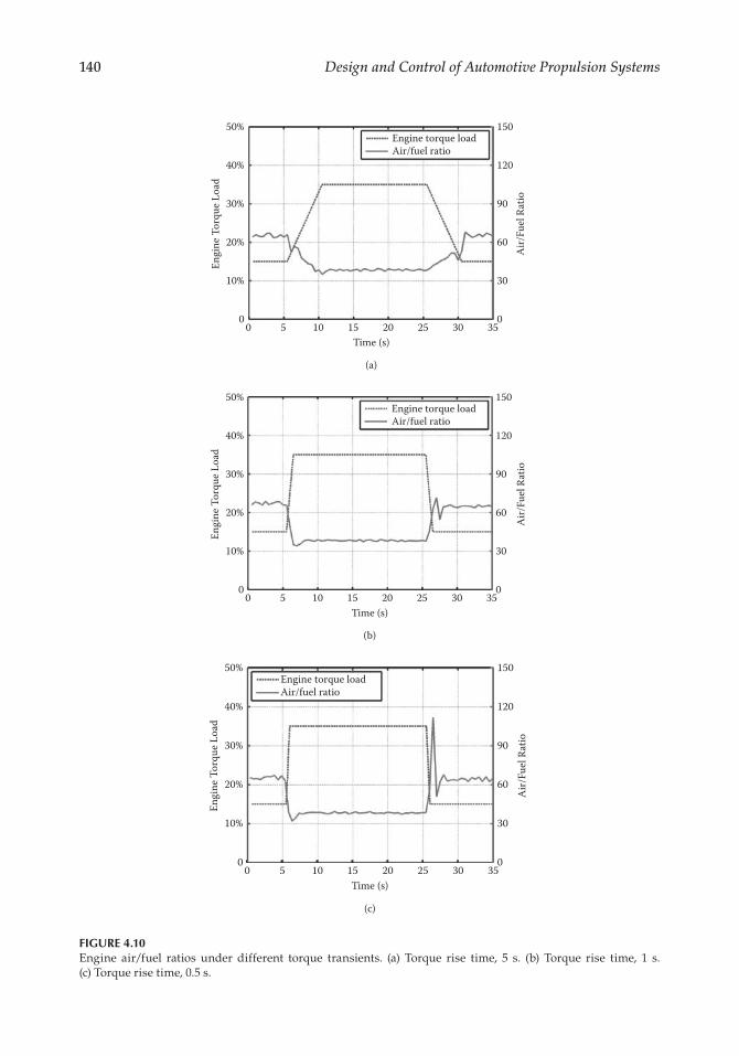
140 Design and Control of Automotive Propulsion Systems
50%
40%
30%
20%
10%
00 5 10 15
Time (s)
Engi
ne T
orqu
e Loa
d
Air/
Fuel
Rat
io
Air/fuel ratioEngine torque load
20 25 30 350
30
60
90
120
150
(a)
50%
40%
30%
20%
10%
00 5 10 15
Time (s)
Engi
ne T
orqu
e Loa
d
Air/
Fuel
Rat
io
Air/fuel ratioEngine torque load
20 25 30 350
30
60
90
120
150
(b)
Time (s)
50%
40%
30%
20%
10%
00 5 10 15
Engi
ne T
orqu
e Loa
d
Air/
Fuel
Rat
io
Engine torque load
20 25 30 350
30
60
90
120
150
Air/fuel ratio
(c)
FIGURE 4.10Engine air/fuel ratios under different torque transients. (a) Torque rise time, 5 s. (b) Torque rise time, 1 s. (c) Torque rise time, 0.5 s.
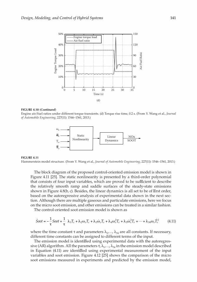
141Design, Modeling, and Control of Hybrid Systems
The block diagram of the proposed control-oriented emission model is shown in Figure 4.11 [25]. The static nonlinearity is presented by a third-order polynomial that consists of four input variables, which are proved to be sufficient to describe the relatively smooth ramp and saddle surfaces of the steady-state emissions shown in Figure 4.8(b, c). Besides, the linear dynamics is all set to be of first order, based on the autoregressive analysis of experimental data shown in the next sec-tion. Although there are multiple gaseous and particulate emissions, here we focus on the micro soot emission, and other emissions can be treated in a similar fashion.
The control-oriented soot emission model is shown as
Soot Soot T T T T T Te e e e e e e e e e e= −τ
+τλ + λ ω + λ ω + λ ω + λ ω + + λ ω� � � � �1 1
1 2 3 42
52
342 (4.11)
where the time constant τ and parameters λ1,…, λ34 are all constants. If necessary, different time constants can be assigned to different terms of the input.
The emission model is identified using experimental data with the autoregres-sive (AR) algorithm. All the parameters τ, λ1,…, λ34 in the emission model described in Equation (4.11) are identified using experimental measurement of the input variables and soot emission. Figure 4.12 [25] shows the comparison of the micro soot emissions measured in experiments and predicted by the emission model,
50%
40%
30%
20%
10%
00 5 10 15
Time (s)
Engi
ne T
orqu
e Loa
d
Air/
Fuel
Rat
io
Engine torque load
20 25 30 350
30
60
90
120
150
Air/fuel ratio
(d)
FIGURE 4.10 (Continued)Engine air/fuel ratios under different torque transients. (d) Torque rise time, 0.2 s. (From Y. Wang et al., Journal of Automobile Engineering, 227(11): 1546–1561, 2013.)
StaticNonlinearity
LinearDynamics
NOxSOOT
ωe
ωe
Te
Te
FIGURE 4.11Hammerstein model structure. (From Y. Wang et al., Journal of Automobile Engineering, 227(11): 1546–1561, 2013.)
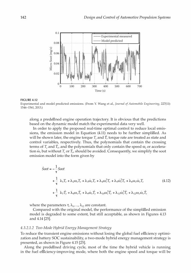
142 Design and Control of Automotive Propulsion Systems
along a predefined engine operation trajectory. It is obvious that the predictions based on the dynamic model match the experimental data very well.
In order to apply the proposed real-time optimal control to reduce local emis-sions, the emission model in Equation (4.11) needs to be further simplified. As will be shown later, the engine torque Te and Te
� torque rate are treated as state and control variables, respectively. Thus, the polynomials that contain the crossing terms of Te and Te
� , and the polynomials that only contain the speed ωe or accelera-tion eω� but without Te or Te
� , should be avoided. Consequently, we simplify the soot emission model into the form given by
Soot Soot
T T T T T T
T T T T T T
e e e e e e e e e e e e
e e e e e e e e e e e e
= −τ
+τλ + λ ω + λ ω + λ ω + λ ω + λ ω ω
+τλ + λ ω + λ ω + λ ω + λ ω + λ ω ω
�
� � �
� � � � � � � � �
1
1
1
1 2 3 42
52
6
7 8 9 102
112
12
(4.12)
where the parameters τ, λ1,…, λ12 are constant. Compared with the original model, the performance of the simplified emission
model is degraded to some extent, but still acceptable, as shown in Figures 4.13 and 4.14 [25].
4.3.2.1.2 Two-Mode Hybrid Energy Management Strategy
To reduce the transient engine emissions without losing the global fuel efficiency optimi-zation and battery SOC sustainability, a two-mode hybrid energy management strategy is presented, as shown in Figure 4.15 [25].
Along the predefined driving cycle, most of the time the hybrid vehicle is running in the fuel efficiency-improving mode, where both the engine speed and torque will be
0.1
0.08
0.06
0.04
0.02
00 100 200 300
Time (s)
Experimental measuredModel predicted
Mic
ro S
oot (
mg/
s)
400 500 600 700
FIGURE 4.12Experimental and model predicted emissions. (From Y. Wang et al., Journal of Automobile Engineering, 227(11): 1546–1561, 2013.)
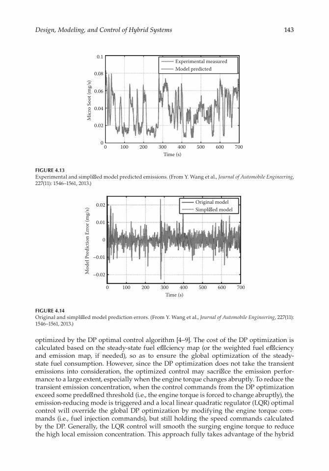
143Design, Modeling, and Control of Hybrid Systems
optimized by the DP optimal control algorithm [4–9]. The cost of the DP optimization is calculated based on the steady-state fuel efficiency map (or the weighted fuel efficiency and emission map, if needed), so as to ensure the global optimization of the steady-state fuel consumption. However, since the DP optimization does not take the transient emissions into consideration, the optimized control may sacrifice the emission perfor-mance to a large extent, especially when the engine torque changes abruptly. To reduce the transient emission concentration, when the control commands from the DP optimization exceed some predefined threshold (i.e., the engine torque is forced to change abruptly), the emission-reducing mode is triggered and a local linear quadratic regulator (LQR) optimal control will override the global DP optimization by modifying the engine torque com-mands (i.e., fuel injection commands), but still holding the speed commands calculated by the DP. Generally, the LQR control will smooth the surging engine torque to reduce the high local emission concentration. This approach fully takes advantage of the hybrid
0.1
0.08
0.06
0.04
0.02
00 100 200 300
Time (s)
Experimental measuredModel predicted
Mic
ro S
oot (
mg/
s)
400 500 600 700
FIGURE 4.13Experimental and simplified model predicted emissions. (From Y. Wang et al., Journal of Automobile Engineering, 227(11): 1546–1561, 2013.)
0.02
0.01
0
–0.01
–0.02
0 100 200 300Time (s)
Original modelSimpli�ed model
Mod
el P
redi
ctio
n Er
ror (
mg/
s)
400 500 600 700
FIGURE 4.14Original and simplified model prediction errors. (From Y. Wang et al., Journal of Automobile Engineering, 227(11): 1546–1561, 2013.)
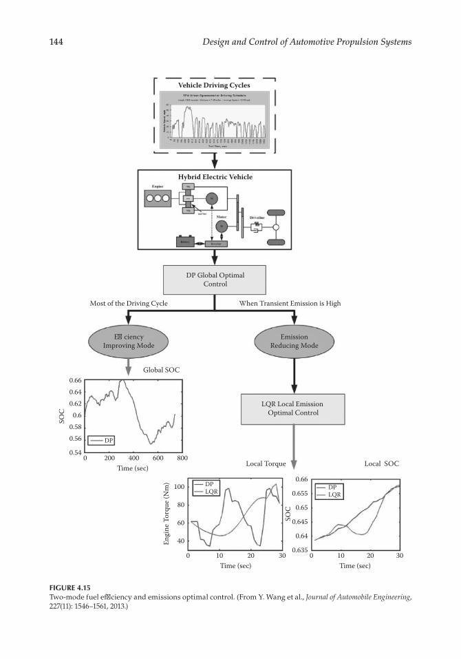
144 Design and Control of Automotive Propulsion Systems
Vehicle Driving Cycles
Hybrid Electric Vehicle
DP Global OptimalControl
LQR Local Emission Optimal Control
When Transient Emission is HighMost of the Driving Cycle
EmissionReducing Mode
E�ciencyImproving Mode
Global SOC
DP
SOC
Time (sec)4002000
0.66
0.64
0.62
0.6
0.58
0.56
0.54800600
SOC
Time (sec)100
0.66
0.655
0.65
0.645
0.64
0.6353020
DPLQR
DPLQR
Engi
ne T
orqu
e (N
m)
Time (sec)100
100
80
60
40
3020
Local Torque Local SOC
FIGURE 4.15Two-mode fuel efficiency and emissions optimal control. (From Y. Wang et al., Journal of Automobile Engineering, 227(11): 1546–1561, 2013.)

145Design, Modeling, and Control of Hybrid Systems
powertrain system where the electric torques can be flexibly controlled to compensate the deficit engine torque at any time instant so as to keep tracking the predefined engine speed trajectory. At the end of the time horizon, the battery SOC of the hybrid vehicle will be driven back to the globally optimized point, so that the global fuel efficiency optimiza-tion and battery SOC sustainability can still be maintained. The design of the two-mode hybrid energy management strategy is shown in detail as follows:
1. Hybrid powertrain system dynamics. A typical power-split hybrid powertrain system (THS II), where a planetary gear set is employed as the core mechanism, is shown in Figure 4.16 [25]. The dynamic models for the power-split hybrid system have been shown in Section 4.3.1.
With respect to the optimal target, the powertrain dynamics in Equations (4.1) to (4.8) can be written by a compact form:
2
4
2
2
1
3
1
4
1
4
1
2
2
1
3
1
4
1
4
1
2
2 1 2( )
( )
( )
ω = + + − αω +β
ω = + + − αω +β
= − +− − ω η + ω η
�
�
�
aa
Taa
Taa
Taa
bb
Tbb
Tbb
Tbb
SOCV
Q R
V T T R
Q R
v e g m v
e e g m v
batt
batt batt
batt g g gk
m m mk
batt
batt batt
(4.13)
where
ωm = ωv Kratio
ωgS + ωmR = ωe (R + S)
The parameters a1 to a4, b1 to b4 are explained in [15] in detail. 2. Efficiency-improving mode: global DP optimization. In the efficiency-improving
mode, dynamic programming, which has been widely investigated in the hybrid
Engine RingTransmission
Generator
Sun
CarrierMotor Driveline
ωv Tv
InverterBattery
Tmωm
ωmTeωe
Tgωg
M
M
Ring
FIGURE 4.16Power-split hybrid powertrain system. (From Y. Wang et al., Journal of Automobile Engineering, 227(11): 1546–1561, 2013.)
146 Design and Control of Automotive Propulsion Systems
powertrain control area [4–9], is utilized as the energy management strategy. DP is a global optimization algorithm that backward searches all the possible states and feasible control actions along a predefined path, so as to find the optimal operation trajectory to meet the specific optimization objective (cost function).
The cost function used in the DP optimization is designed to minimize the fuel consumption and keep the SOC sustained in a limited bound, given by
J FC k f SOC N SOC N
m SOC N SOC N
k
N
soc des
soc des
0
12∑{ }( ) ( ) ( )
( ) ( )
= + −
− −
=
−
(4.14)
where FC is the fuel consumption in a single sampling step, SOC(N) and SOC(N)des are the actual and desired battery SOC at the final step, fsoc is the SOC sustaining factor, and msoc is the SOC variation compensation factor. Usually, fsoc will be given by a large value to force the SOC to converge to the desired value at the end; msoc will be estimated based on the actual equivalent fuel consumption from the SOC deviation.
3. Emission-reducing mode: local LQR optimal control. In the emission-reducing mode, a local optimal control algorithm is required to realize two tasks:
a. It modifies the engine torque trajectory to realize the local emission optimiza-tion, without changing the engine speed during the local time horizon.
b. At the end of the local time horizon, the battery SOC should be driven back to the trajectory defined by the DP, so that the SOC sustainability provided by the DP can still be maintained.
To meet the above requirements, a linear quadratic regulator is utilized in the emission-reducing mode. LQR is a linear state feedback optimal control along some finite time period [22]. Thus, the linearization and necessary simplification of the nonlinear plant model, which includes the powertrain dynamics in Equation (4.13) and emission dynamics in Equation (4.12), are necessary.
For the engine and vehicle dynamics, the engine speed and vehicle speed will be maintained the same as the DP-optimized results; in other words, both ωe and ωv, as well as their time derivative, can be treated as known terms in the LQR control. Then the nonlinear terms involved with ωe and ωv in Equation (4.13) are actually eliminated, and we can rewrite the engine and vehicle dynamics as
Ta b b aa b b a
Ta b b a
a b b a
r T r
Ta b b aa b b a
Ta b b a
a b b a
r T r
m ev e
v
m e m
g ev e
g e g
2 3 2 3
4 3 4 3
1 3 1 3
4 3 4 3
2
1 2
2 4 2 4
3 4 3 4
1 4 1 4
3 4 3 4
1 2
( )= −−−
+ω − ω
−+ αω +β
= +
= −−−
+ω − ω
−
= +
� �
� � (4.15)
147Design, Modeling, and Control of Hybrid Systems
For the battery dynamics, if we neglect the internal resistance of the battery, the nonlinear dynamics can be transformed into a linear form:
SOCP
V QT T
V Q
r T rR S K R
SV Q
r T r KV Q
batt
batt batt
g g gk
m m mk
batt batt
g e ge v ratio
gk
batt batt
m e m v ratio mk
batt batt
1 2
1 21
1 22
( ) ( )
( )( )
= − = −− ω η + ω η
=
+ω + − ω
η
−+ ω η
�
(4.16)
For the micro soot emission model shown in Equation (4.12), since the engine speed and its time derivative are both considered known parameters, the emission dynamics can be expressed by a more compact equation:
1 1, ,
1, ,
1 6
7 12
( ) ( )
( ) ( )
= −τ
+τ
ω ω + + ω ω
+τ
ω ω + + ω ω
� � � �
� � � �
Soot Soot f f T
f f T
e e e e e
e e e e e
(4.17)
where the functions f1,…, f6 are λ 1, λ 2ωe, e3λ ω� , e42λ ω , e5
2λ ω� , and e e6λ ω ω� , respec-
tively, and the functions f7,…, f12 are λ 7, λ 8ωe, e9λ ω� , e102λ ω , e11
2λ ω� , and e e12λ ω ω� , respectively.
Further, combining Equations (4.15) to (4.17) yields a complete description of the engine soot emission dynamics (here a discrete-time form is used for the discrete-time LQR control):
x(K + 1) = A(K) x(K) + B(K) u(K) + G(K)
or
x K A K A KA K
x K
B K u K
G K
11 0 0
00 1
1
0
0
0
21 22
31
2
3
( ) ( ) ( )( )
( )
( ) ( )
( )
+ =
+ +
(4.18)
148 Design and Control of Automotive Propulsion Systems
where the x(K) = [Te(K) Soot(K) SOC(K)]T states and the input u(K) = dTe(K), which is the torque change from the Kth step to the (K + 1)th step. Other parameters are defined as
1, ,
11
1, ,
( ) ( )
( )
21 1 6
22
31
1
1
2 7 12
3
2
2
1
2
1
2
( )
( )
( )
( ) ( )
( ) ( )
( )
( )( ) ( )
( ) ( )
( )
( )
=τ
ω ω + + ω ω
= −τ
=
ω + − ωη
−ω η
=τ
ω ω + + ω ω
=
ω + − ωη
−ω η
� � �
� � �
A f f
A
Ar
K R S K K RS
V Q
r K K
V Q
B f f
Gr
K R S K K RS
V Q
r K KV Q
e e e e
ge v ratio
gk
batt batt
m v ratio mk
batt batt
e e e e
ge v ratio
gk
batt batt
m e v ratio mk
batt batt
(4.19)
After transforming the original nonlinear plant model into the linear form in Equation (4.18), the LQR optimal control algorithm can be designed. The optimal objective of the LQR control is to minimize the cost function within a predefined time period (in the discrete-time form, correspondingly, K = 0, …, N):
J x N Hx N x K Q K x K u K Ru KT T T T
K
N12
12
0
1
∑( ) ( ) ( ) ( ) ( ) ( ) ( )= + +=
−
(4.20)
where the gain matrices H, Q, and R can be customized to meet the specific opti-mal target.
With the objective of minimizing the soot emission by smoothing the torque change, as well as maintaining the battery SOC the same as the DP result at the final stage, the gain matrices H, Q, and R are designed as follows:
,0
0,
1
2
3
2 1= = =Hh
hh
Q q R r
These gain matrices need to be tuned to produce a good balance of the soot emission minimization and battery SOC sustainability. Usually, h3 is much larger
149Design, Modeling, and Control of Hybrid Systems
than h1 and h2 for driving the SOC convergence to the predefined value; q2 needs to be tuned carefully to reduce the soot emission during the time horizon; and r1 can be quite small (since the effects of the torque transients on the soot emission have been contained in the dynamics of state x2 and penalized by matrix Q). For example, a group of typical parameters is given by h1 = 0.01, h2 = 1, h3 = 1e7, q2 = 5000, and r1 = 0.01.
Then the LQR state feedback control law u* can be generated as
u N K F N K x N K
G N K
*
0
0
3
( ) ( ) ( )
( )
− = − − +
−
(4.21)
where
F(N − K) = −[R + BT(N − K) P(K) B(N − K)]−1
× BT(N − K) P(K) A(N − K)
P(K + 1) = [A(N − K) + B(N − K) F(N − K)]T P(K) (4.22)
× [A(N − K) + B(N − K) F(N − K)]
+ FT(N − K) RF(N − K)] + Q
The generated LQR optimal control law is not the same as the standard form because of the existence of the known time-varying term G. However, the special form of the matrices A, G, and Q (which satisfies AG = G and GTQG = 0) allows us to modify the control law without violating the derivation of the closed-loop form of the LQR control law.
4.3.2.1.3 Experimental Results and Analysis
To demonstrate the performance of the proposed two-mode hybrid energy management strategy, a large number of experimental studies have been conducted under a high-fidelity hybrid powertrain testing environment. In particular, a rapid prototyping hybrid powertrain research platform was employed [23, 24]. With the hardware-in-the-loop (HIL) engine testing architecture, this research platform utilized a high-bandwidth hydrostatic dynamometer to precisely mimic the dynamic behaviors of the tested hybrid powertrain system to interact with a real-world John Deere 4045HF Tier IV diesel engine, so as to create the high-fidelity engine operations as if it were under the actual HEV dynamic environment, as shown in Figure 4.17(a) [25]. On this basis, state-of-the-art transient fuel consumption and emission measurement instruments (including the AVL P402 Fuel Measurement System, AVL Micro Soot Sensing System, and AVL FTIR Emission Sampling and Measurement System) were employed for system output measurements, as shown in Figure 4.17(b) [25].
The basic principle of switching between the two operation modes is, since the fuel efficiency is not considered in the LQR control, both the local time horizon and
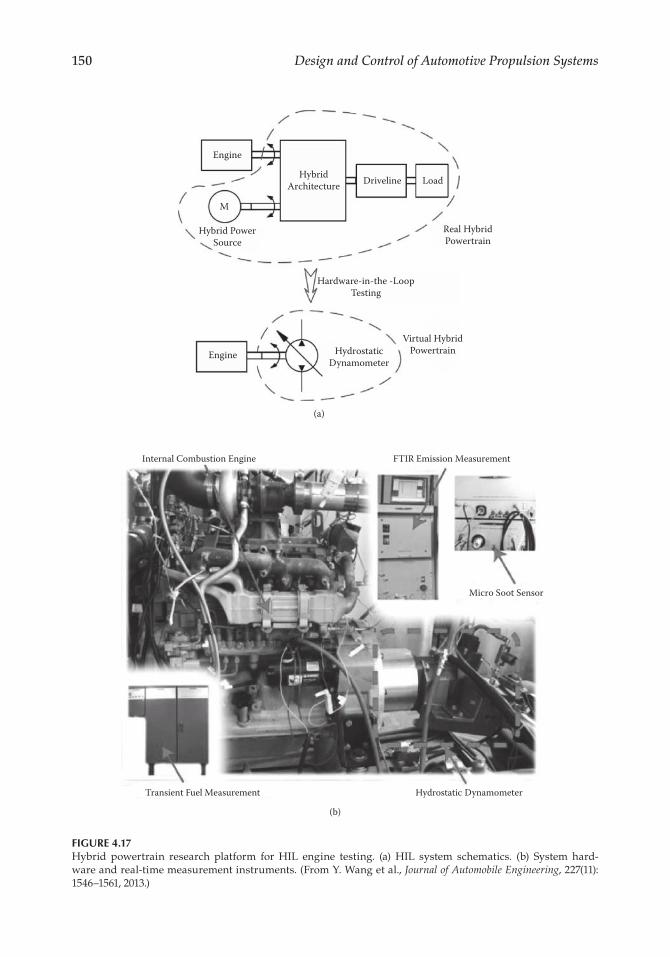
150 Design and Control of Automotive Propulsion Systems
Engine
Engine
HybridArchitecture Driveline Load
Real HybridPowertrain
Hardware-in-the -LoopTesting
Virtual HybridPowertrainHydrostatic
Dynamometer
Hybrid PowerSource
M
(a)
Transient Fuel Measurement Hydrostatic Dynamometer
Micro Soot Sensor
FTIR Emission MeasurementInternal Combustion Engine
(b)
FIGURE 4.17Hybrid powertrain research platform for HIL engine testing. (a) HIL system schematics. (b) System hard-ware and real-time measurement instruments. (From Y. Wang et al., Journal of Automobile Engineering, 227(11): 1546–1561, 2013.)
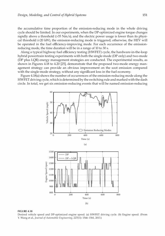
151Design, Modeling, and Control of Hybrid Systems
the accumulative time proportion of the emission-reducing mode in the whole driving cycle should be limited. In our experiments, when the DP-optimized engine torque changes rapidly above a threshold (>35 Nm/s), and the electric power usage is lower than its physi-cal threshold (<20 kW), the emission-reducing mode is triggered; otherwise, the HEV will be operated in the fuel efficiency-improving mode. For each occurrence of the emission-reducing mode, the time duration will be in a range of 10 to 30 s.
Along a typical highway fuel efficiency testing (HWFET) cycle, the hardware-in-the-loop hybrid powertrain testing experiments with both the single-mode (DP only) and two-mode (DP plus LQR) energy management strategies are conducted. The experimental results, as shown in Figures 4.18 to 4.20 [25], demonstrate that the proposed two-mode energy man-agement strategy can provide an obvious improvement on the soot emission compared with the single-mode strategy, without any significant loss in the fuel economy.
Figure 4.18(a) shows the number of occurrences of the emission-reducing mode along the HWFET driving cycle, which is determined by the switching rule and marked with the dash circle. In total, we get six emission-reducing events that will be named emission-reducing
Emission Reducing Modes
0 200 400Time (s)
Vehi
cle S
peed
(mph
)
600 800
60
50
40
30
20
(a)
1500DPDP + LQR
0 200 400Time (s)
Engi
ne S
peed
(rpm
)
600 800
1400
1300
1200
1100
1000
900
800
(b)
FIGURE 4.18Desired vehicle speed and DP-optimized engine speed. (a) HWFET driving cycle. (b) Engine speed. (From Y. Wang et al., Journal of Automobile Engineering, 227(11): 1546–1561, 2013.)

152 Design and Control of Automotive Propulsion Systems
200DPDP + LQR
0 200 400Time (s)
Engi
ne T
orqu
e (N
m)
600 800
150
100
50
0
(a)
0.7DPDP + LQR
0 200 400Time (s)
Batte
ry S
OC
(1)
600 800
0.65
0.6
0.55
0.5
(b)
0.12DPDP + LQR
0 200 400Time (s)
Mic
ro S
oot (
mg/
s)
600 800
0.1
0.08
0.06
0.04
0.02
0
(c)
FIGURE 4.19Globally and locally optimized trajectory along the HWFET cycle. (a) Engine torques. (b) Battery SOC. (c) Micro soot emission.
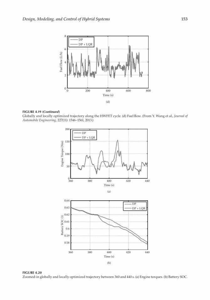
153Design, Modeling, and Control of Hybrid Systems
8DPDP + LQR
0 200 400Time (s)
Fuel
Flo
w (L
/h)
600 800
6
4
2
0
(d)
FIGURE 4.19 (Continued)Globally and locally optimized trajectory along the HWFET cycle. (d) Fuel flow. (From Y. Wang et al., Journal of Automobile Engineering, 227(11): 1546–1561, 2013.)
200DPDP + LQR
360 380 400Time (s)
Engi
ne T
orqu
e (N
m)
420 440
150
100
50
0
(a)
0.64DPDP + LQR
360 380 400Time (s)
Batte
ry S
OC
(1)
420 440
0.62
0.61
0.63
0.6
0.59
0.58
(b)
FIGURE 4.20Zoomed-in globally and locally optimized trajectory between 360 and 440 s. (a) Engine torques. (b) Battery SOC.
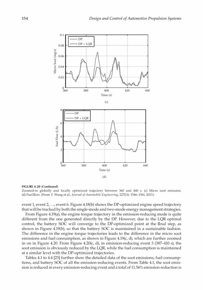
154 Design and Control of Automotive Propulsion Systems
event 1, event 2, …, event 6. Figure 4.18(b) shows the DP-optimized engine speed trajectory that will be tracked by both the single-mode and two-mode energy management strategies.
From Figure 4.19(a), the engine torque trajectory in the emission-reducing mode is quite different from the one generated directly by the DP. However, due to the LQR optimal control, the battery SOC will converge to the DP-optimized point at the final step, as shown in Figure 4.19(b), so that the battery SOC is maintained in a sustainable fashion. The difference in the engine torque trajectories leads to the difference in the micro soot emissions and fuel consumption, as shown in Figure 4.19(c, d), which are further zoomed in on in Figure 4.20. From Figure 4.20(c, d), in emission-reducing event 3 (387–410 s), the soot emission is obviously reduced by the LQR, while the fuel consumption is maintained at a similar level with the DP-optimized trajectories.
Tables 4.1 to 4.4 [25] further show the detailed data of the soot emissions, fuel consump-tions, and battery SOC of all the emission-reducing events. From Table 4.1, the soot emis-sion is reduced in every emission-reducing event and a total of 11.56% emission reduction is
0.1DPDP + LQR
360 380 400Time (s)
Mic
ro S
oot (
mg/
s)
420 440
0.08
0.06
0.04
0.02
0
(c)
8DPDP + LQR
360 380 400Time (s)
Fuel
Flo
w (L
/h)
420 440
6
4
2
0
(d)
FIGURE 4.20 (Continued)Zoomed-in globally and locally optimized trajectory between 360 and 440 s. (c) Micro soot emission. (d) Fuel flow. (From Y. Wang et al., Journal of Automobile Engineering, 227(11): 1546–1561, 2013.)
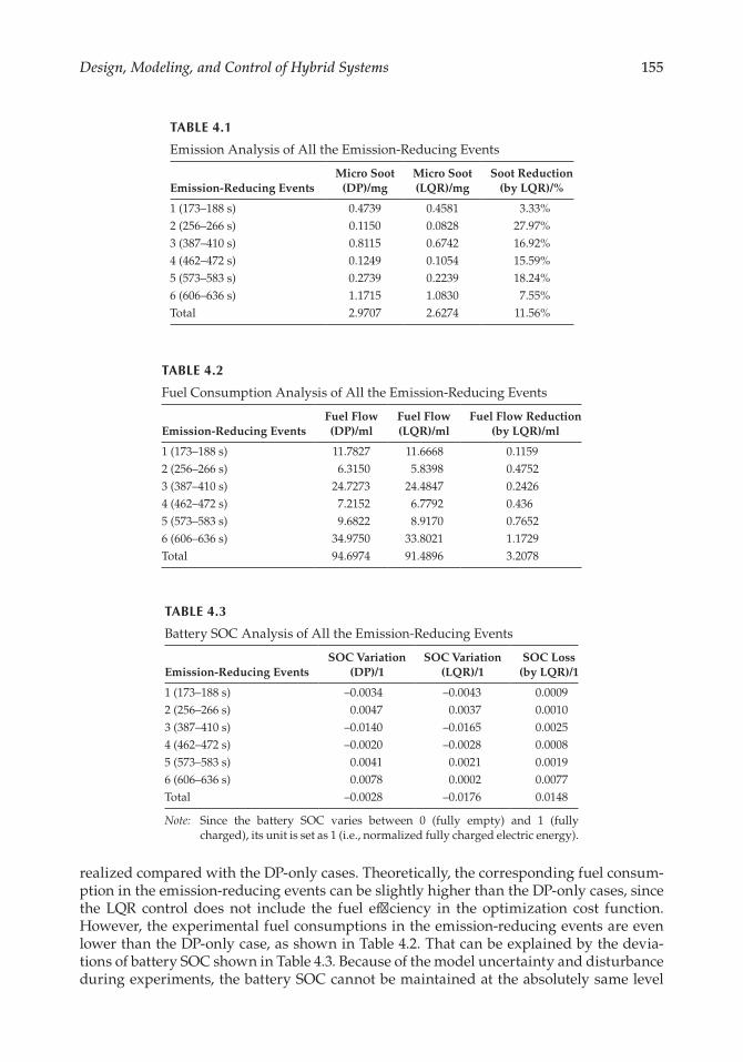
155Design, Modeling, and Control of Hybrid Systems
realized compared with the DP-only cases. Theoretically, the corresponding fuel consum-ption in the emission-reducing events can be slightly higher than the DP-only cases, since the LQR control does not include the fuel efficiency in the optimization cost function. However, the experimental fuel consumptions in the emission-reducing events are even lower than the DP-only case, as shown in Table 4.2. That can be explained by the devia-tions of battery SOC shown in Table 4.3. Because of the model uncertainty and disturbance during experiments, the battery SOC cannot be maintained at the absolutely same level
TABLE 4.1
Emission Analysis of All the Emission-Reducing Events
Emission-Reducing EventsMicro Soot
(DP)/mgMicro Soot(LQR)/mg
Soot Reduction(by LQR)/%
1 (173–188 s) 0.4739 0.4581 3.33%2 (256–266 s) 0.1150 0.0828 27.97%3 (387–410 s) 0.8115 0.6742 16.92%4 (462–472 s) 0.1249 0.1054 15.59%5 (573–583 s) 0.2739 0.2239 18.24%6 (606–636 s) 1.1715 1.0830 7.55%Total 2.9707 2.6274 11.56%
TABLE 4.2
Fuel Consumption Analysis of All the Emission-Reducing Events
Emission-Reducing EventsFuel Flow(DP)/ml
Fuel Flow(LQR)/ml
Fuel Flow Reduction(by LQR)/ml
1 (173–188 s) 11.7827 11.6668 0.11592 (256–266 s) 6.3150 5.8398 0.47523 (387–410 s) 24.7273 24.4847 0.24264 (462–472 s) 7.2152 6.7792 0.4365 (573–583 s) 9.6822 8.9170 0.76526 (606–636 s) 34.9750 33.8021 1.1729Total 94.6974 91.4896 3.2078
TABLE 4.3
Battery SOC Analysis of All the Emission-Reducing Events
Emission-Reducing EventsSOC Variation
(DP)/1SOC Variation
(LQR)/1SOC Loss
(by LQR)/1
1 (173–188 s) –0.0034 –0.0043 0.00092 (256–266 s) 0.0047 0.0037 0.00103 (387–410 s) –0.0140 –0.0165 0.00254 (462–472 s) –0.0020 –0.0028 0.00085 (573–583 s) 0.0041 0.0021 0.00196 (606–636 s) 0.0078 0.0002 0.0077Total –0.0028 –0.0176 0.0148
Note: Since the battery SOC varies between 0 (fully empty) and 1 (fully charged), its unit is set as 1 (i.e., normalized fully charged electric energy).
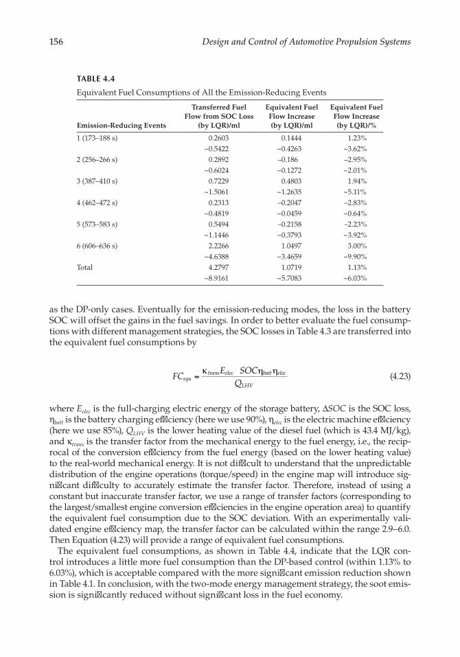
156 Design and Control of Automotive Propulsion Systems
as the DP-only cases. Eventually for the emission-reducing modes, the loss in the battery SOC will offset the gains in the fuel savings. In order to better evaluate the fuel consump-tions with different management strategies, the SOC losses in Table 4.3 are transferred into the equivalent fuel consumptions by
FCE SOC
Qequ
trans elec batt elec
LHV=κ η η
(4.23)
where Eelec is the full-charging electric energy of the storage battery, ΔSOC is the SOC loss, ηbatt is the battery charging efficiency (here we use 90%), ηelec is the electric machine efficiency (here we use 85%), QLHV is the lower heating value of the diesel fuel (which is 43.4 MJ/kg), and κtrans is the transfer factor from the mechanical energy to the fuel energy, i.e., the recip-rocal of the conversion efficiency from the fuel energy (based on the lower heating value) to the real-world mechanical energy. It is not difficult to understand that the unpredictable distribution of the engine operations (torque/speed) in the engine map will introduce sig-nificant difficulty to accurately estimate the transfer factor. Therefore, instead of using a constant but inaccurate transfer factor, we use a range of transfer factors (corresponding to the largest/smallest engine conversion efficiencies in the engine operation area) to quantify the equivalent fuel consumption due to the SOC deviation. With an experimentally vali-dated engine efficiency map, the transfer factor can be calculated within the range 2.9–6.0. Then Equation (4.23) will provide a range of equivalent fuel consumptions.
The equivalent fuel consumptions, as shown in Table 4.4, indicate that the LQR con-trol introduces a little more fuel consumption than the DP-based control (within 1.13% to 6.03%), which is acceptable compared with the more significant emission reduction shown in Table 4.1. In conclusion, with the two-mode energy management strategy, the soot emis-sion is significantly reduced without significant loss in the fuel economy.
TABLE 4.4
Equivalent Fuel Consumptions of All the Emission-Reducing Events
Emission-Reducing Events
Transferred Fuel Flow from SOC Loss
(by LQR)/ml
Equivalent Fuel Flow Increase(by LQR)/ml
Equivalent Fuel Flow Increase(by LQR)/%
1 (173–188 s) 0.2603 0.1444 1.23%~0.5422 ~0.4263 ~3.62%
2 (256–266 s) 0.2892 –0.186 –2.95%~0.6024 ~0.1272 ~2.01%
3 (387–410 s) 0.7229 0.4803 1.94%~1.5061 ~1.2635 ~5.11%
4 (462–472 s) 0.2313 –0.2047 –2.83%~0.4819 ~0.0459 ~0.64%
5 (573–583 s) 0.5494 –0.2158 –2.23%~1.1446 ~0.3793 ~3.92%
6 (606–636 s) 2.2266 1.0497 3.00%~4.6388 ~3.4659 ~9.90%
Total 4.2797 1.0719 1.13%~8.9161 ~5.7083 ~6.03%
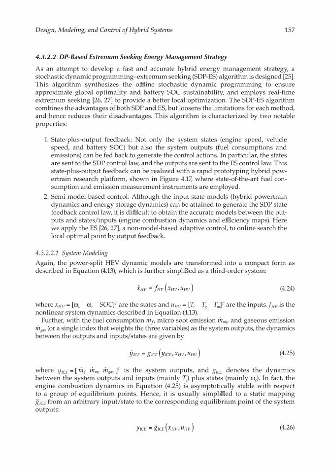
157Design, Modeling, and Control of Hybrid Systems
4.3.2.2 DP-Based Extremum Seeking Energy Management Strategy
As an attempt to develop a fast and accurate hybrid energy management strategy, a stochastic dynamic programming–extremum seeking (SDP-ES) algorithm is designed [25]. This algorithm synthesizes the offline stochastic dynamic programming to ensure approximate global optimality and battery SOC sustainability, and employs real-time extremum seeking [26, 27] to provide a better local optimization. The SDP-ES algorithm combines the advantages of both SDP and ES, but loosens the limitations for each method, and hence reduces their disadvantages. This algorithm is characterized by two notable properties:
1. State-plus-output feedback: Not only the system states (engine speed, vehicle speed, and battery SOC) but also the system outputs (fuel consumptions and emissions) can be fed back to generate the control actions. In particular, the states are sent to the SDP control law, and the outputs are sent to the ES control law. This state-plus-output feedback can be realized with a rapid prototyping hybrid pow-ertrain research platform, shown in Figure 4.17, where state-of-the-art fuel con-sumption and emission measurement instruments are employed.
2. Semi-model-based control: Although the input state models (hybrid powertrain dynamics and energy storage dynamics) can be attained to generate the SDP state feedback control law, it is difficult to obtain the accurate models between the out-puts and states/inputs (engine combustion dynamics and efficiency maps). Here we apply the ES [26, 27], a non-model-based adaptive control, to online search the local optimal point by output feedback.
4.3.2.2.1 System Modeling
Again, the power-split HEV dynamic models are transformed into a compact form as described in Equation (4.13), which is further simplified as a third-order system:
,( )=�x f x uHV HV HV HV (4.24)
where xHV = [ωv ωe SOC]T are the states and uHV = [Te Tg Tm]T are the inputs. fHV is the nonlinear system dynamics described in Equation (4.13).
Further, with the fuel consumption mf� , micro soot emission mms� , and gaseous emission mgas� (or a single index that weights the three variables) as the system outputs, the dynamics between the outputs and inputs/states are given by
, ,( )=�y g y x uICE ICE ICE HV HV (4.25)
where y m m mICE f ms gasT[ ]= � � � is the system outputs, and gICE denotes the dynamics
between the system outputs and inputs (mainly Te) plus states (mainly ωe). In fact, the engine combustion dynamics in Equation (4.25) is asymptotically stable with respect to a group of equilibrium points. Hence, it is usually simplified to a static mapping gICE from an arbitrary input/state to the corresponding equilibrium point of the system outputs:
,( )=y g x uICE ICE HV HV (4.26)

158 Design and Control of Automotive Propulsion Systems
4.3.2.2.2 Analysis of the Real-Time Energy Management Strategies
4.3.2.2.2.1 Existing Real-Time Hybrid Energy Optimization Algorithms Various hybrid energy optimization algorithms have been studied. The rule-based control [4, 5] employs a set of event-triggered rules to control the hybrid powertrain for high fuel efficiency, but it provides no guarantee of global optimality. The A-ECMS strategy [3, 10] converses the instantaneous electric power into the estimated equivalent fuel consumption to realize the instantaneous minimization of the gross fuel consumptions. A-ECMS simplifies the optimization problem; however, its optimality depends on the choice (or adaption) of the precise energy conversion factor, which is very difficult to attain for implementation, albeit existent in theory [28]. The MPC strategy [11, 12] formulates the global optimiza-tion problem into an optimization over a finite time window based on predictive mod-els, and simplifies the nonlinear optimization to a linear quadratic program problem for which the analytical real-time solutions exist. The optimality of the MPC is limited by the assumption of the future vehicle speed (or power demand) in the prediction horizon.
Compared with the above algorithms, the SDP [6–9], which globally optimizes the fuel efficiency by searching all feasible control actions along an infinite time period (with a cost discounting factor) for all the possible states (with estimated probabilities) [6], presents its distinguished advantage in spite of huge offline computation. Theoretically, with the pre-cise statistic knowledge of the future paths, the SDP is able to produce the optimal control in the statistic viewpoint [7]. Thus, it can be chosen as a method to approach the global energy optimal and battery SOC sustainable path.
4.3.2.2.2.2 Limitations of the SDP-Based Optimal Control Even with a good expectation for the global energy optimality, there are some limitations that degrade the theoretical advantage of the SDP algorithm:
1. Curse of dimensionality: When the state variables increase in number, the offline computation load will increase exponentially. This greatly compounds the diffi-culty of the control implementation. Currently, the third-order power-split hybrid dynamic introduces three state variables and induces serious computation prob-lems. To address this, some trade-offs are used to simplify the system models, e.g., limiting the engine power on a predefined curve. However, this will inevitably sacrifice the global optimality to some extent.
2. Negative effect of the large grid size: Similarly, with the purpose of reducing the computation load, the states and inputs are usually discretized with large grid size. This results in the generated optimal controls deviating from the actual opti-mal points due to the rough interpolations in implementation.
3. Lack of the precise system output model: Because of the lack of the complicated engine combustion dynamics, a static engine map that links the engine torque/speed with the fuel consumption is usually used for the offline SDP optimization.
4.3.2.2.3 Optimal Control Design
To make up the inherent deficiencies of the SDP algorithm, an output feedback-based opti-mization tool, extremum seeking (ES), is introduced to locally compensate the SDP optimal control, so as to drive the operating points toward the direction that further reduces fuel consumption. ES is a real-time optimization method that makes use of a periodic perturba-tion to dynamically search a maximum/minimum from an uncertain reference-to-output

159Design, Modeling, and Control of Hybrid Systems
equilibrium map of a dynamic system. This dynamic system can be a nonlinear system if only its equilibrium map has a maximum/minimum, and all the equilibria are locally stable [26, 27].
4.3.2.2.3.1 SDP-ES Optimization Algorithm Design The SDP-ES algorithm utilizes a SDP-based state feedback control as a reference term and injects a local feedback term via ES to compensate the control commands from SDP. The basic schematic of the SDP-ES optimiza-tion is shown in Figure 4.21 [25].
With the state feedback from the HEV system and speed (or power) demands from the driver model, the SDP will search through the control laws in an offline lookup table, to find a corresponding optimal engine power Pe, which further corresponds to an operat-ing point Te e,( )ω
� � on a predefined curve. Here, we call Te e,( )ω
� � the SDP minimum, which
means the minimal fuel consumption point calculated by the SDP. Based on a known SDP minimum, a SOC sustaining line can be generated based on the hybrid vehicle model [29, 30]. The battery SOC of all the points along this line can be maintained the same as the SDP minimum. From Equation (4.17), the SOC sustaining line is the collection of the points that satisfy
P T T T Telec g g gk
m m mk
g g gk
m m mk1 2 1 2= − ω η + ω η = − ω η + ω η
� � � � (4.27)
Power-Split HEV System
mfSDP
Minimum
ESMinimum
SDP State-Feedback Laws
ES Output-Feedback
Adaption Laws
Control Actions uto Reach (ωe, Te)
Te SDPMinimum
Pre-defined Operating Line
SOC Sustain Line
(ωe, Te) on SOC Sustain Line
SDPMinimum
ωe
ωe
ωeHybrid
PowertrainController
yICE (mf)
yICE = gICE (yICE, xHV, uHV)
xHV = fHV (xHV, uHV)
ωv_desxHV (ωv, SOC)
(ωe, Te)
FIGURE 4.21The schematic diagram of the SDP-ES optimization algorithm.
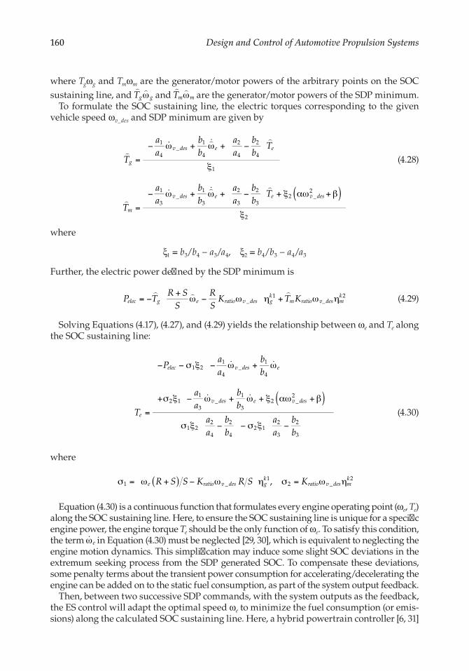
160 Design and Control of Automotive Propulsion Systems
where Tgωg and Tmωm are the generator/motor powers of the arbitrary points on the SOC sustaining line, and Tg gω
� � and Tm mω
� � are the generator/motor powers of the SDP minimum.
To formulate the SOC sustaining line, the electric torques corresponding to the given vehicle speed ωv_des and SDP minimum are given by
T
aa
bb
aa
bb
T
T
aa
bb
aa
bb
T
g
v des e e
m
v des e e v des
1
4_
1
4
2
4
2
4
1
1
3_
1
3
2
3
2
32 _
2
2
( )
=
− ω + ω + −
ξ
=
− ω + ω + − + ξ αω +β
ξ
�� �� �
�� �� �
(4.28)
where
ξ1 = b3/b4 − a3/a4, ξ2 = b4/b3 − a4/a3
Further, the electric power defined by the SDP minimum is
P TR S
SRS
K T Kelec g e ratio v des gk
m ratio v des mk
_1
_2= −
+ω − ω η + ω η
� � � (4.29)
Solving Equations (4.17), (4.27), and (4.29) yields the relationship between ωe and Te along the SOC sustaining line:
T
Paa
bb
aa
bb
aa
bb
aa
bb
e
elec v des e
v des e v des
1 21
4_
1
4
2 11
3_
1
32 _
2
1 22
4
2
42 1
2
3
2
3
( )=
− − σ ξ − ω + ω
+σ ξ − ω + ω + ξ αω +β
σ ξ − − σ ξ −
� �
� �
(4.30)
where
R S S K R S Ke ratio v des gk
ratio v des mk( )σ = ω + − ω η σ = ω η,1 _
12 _
2
Equation (4.30) is a continuous function that formulates every engine operating point (ωe, Te) along the SOC sustaining line. Here, to ensure the SOC sustaining line is unique for a specific engine power, the engine torque Te should be the only function of ωe. To satisfy this condition, the term eω� in Equation (4.30) must be neglected [29, 30], which is equivalent to neglecting the engine motion dynamics. This simplification may induce some slight SOC deviations in the extremum seeking process from the SDP generated SOC. To compensate these deviations, some penalty terms about the transient power consumption for accelerating/decelerating the engine can be added on to the static fuel consumption, as part of the system output feedback.
Then, between two successive SDP commands, with the system outputs as the feedback, the ES control will adapt the optimal speed ωe to minimize the fuel consumption (or emis-sions) along the calculated SOC sustaining line. Here, a hybrid powertrain controller [6, 31]
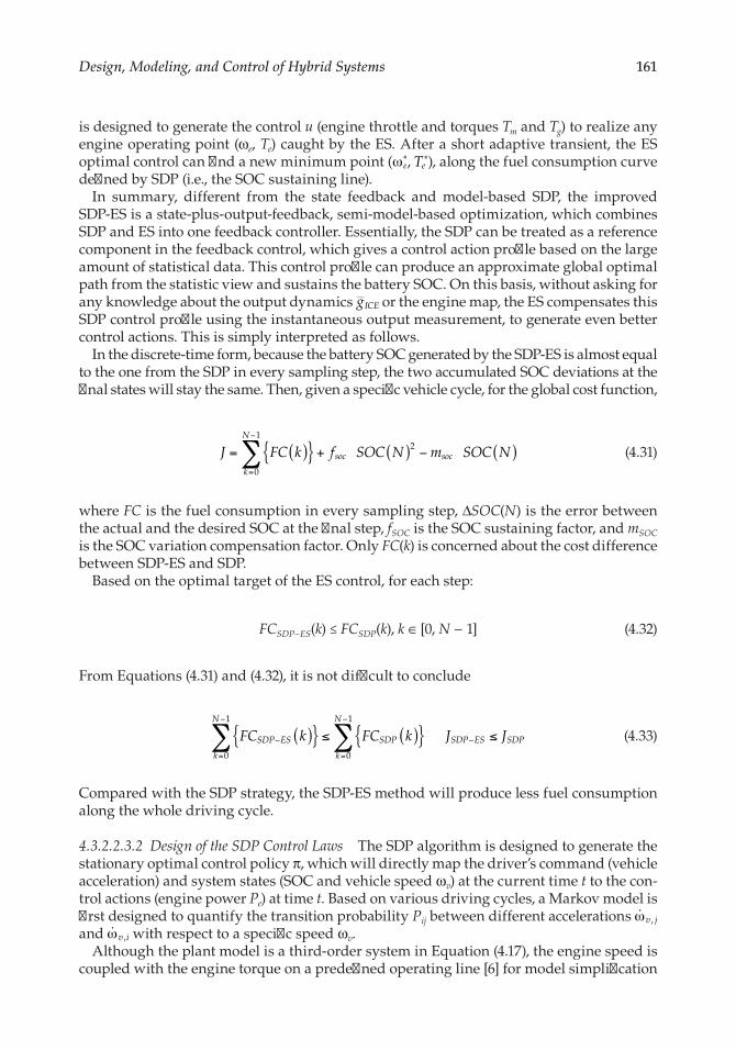
161Design, Modeling, and Control of Hybrid Systems
is designed to generate the control u (engine throttle and torques Tm and Tg) to realize any engine operating point (ωe, Te) caught by the ES. After a short adaptive transient, the ES optimal control can find a new minimum point (ω∗
e, ∗Te ), along the fuel consumption curve defined by SDP (i.e., the SOC sustaining line).
In summary, different from the state feedback and model-based SDP, the improved SDP-ES is a state-plus-output-feedback, semi-model-based optimization, which combines SDP and ES into one feedback controller. Essentially, the SDP can be treated as a reference component in the feedback control, which gives a control action profile based on the large amount of statistical data. This control profile can produce an approximate global optimal path from the statistic view and sustains the battery SOC. On this basis, without asking for any knowledge about the output dynamics gICE or the engine map, the ES compensates this SDP control profile using the instantaneous output measurement, to generate even better control actions. This is simply interpreted as follows.
In the discrete-time form, because the battery SOC generated by the SDP-ES is almost equal to the one from the SDP in every sampling step, the two accumulated SOC deviations at the final states will stay the same. Then, given a specific vehicle cycle, for the global cost function,
∑{ }( ) ( ) ( )= + −=
−
J FC k f SOC N m SOC Nk
N
soc soc
0
12 (4.31)
where FC is the fuel consumption in every sampling step, ΔSOC(N) is the error between the actual and the desired SOC at the final step, fSOC is the SOC sustaining factor, and mSOC is the SOC variation compensation factor. Only FC(k) is concerned about the cost difference between SDP-ES and SDP.
Based on the optimal target of the ES control, for each step:
FCSDP−ES(k) ≤ FCSDP(k), k ∈ [0, N − 1] (4.32)
From Equations (4.31) and (4.32), it is not difficult to conclude
∑ ∑{ } { }( ) ( )≤ ≤−
=
−
=
−
−FC k FC k J JSDP ES
k
N
SDP
k
N
SDP ES SDP
0
1
0
1
(4.33)
Compared with the SDP strategy, the SDP-ES method will produce less fuel consumption along the whole driving cycle.
4.3.2.2.3.2 Design of the SDP Control Laws The SDP algorithm is designed to generate the stationary optimal control policy π, which will directly map the driver’s command (vehicle acceleration) and system states (SOC and vehicle speed ωv) at the current time t to the con-trol actions (engine power Pe) at time t. Based on various driving cycles, a Markov model is first designed to quantify the transition probability Pij between different accelerations v j,ω� and v i,ω� with respect to a specific speed ωv.
Although the plant model is a third-order system in Equation (4.17), the engine speed is coupled with the engine torque on a predefined operating line [6] for model simplification
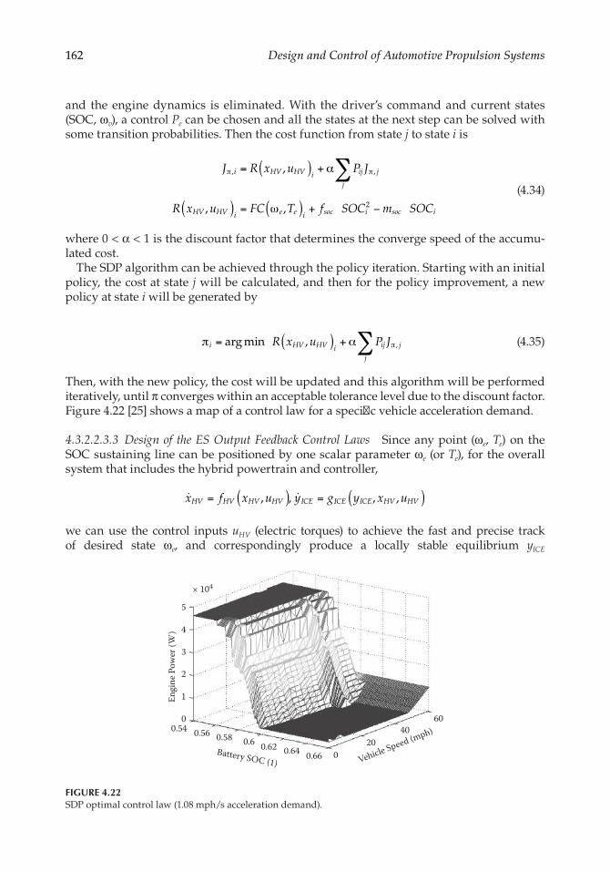
162 Design and Control of Automotive Propulsion Systems
and the engine dynamics is eliminated. With the driver’s command and current states (SOC, ωv), a control Pe can be chosen and all the states at the next step can be solved with some transition probabilities. Then the cost function from state j to state i is
,
, ,
, ,
2
∑( )
( ) ( )
= + α
= ω + −
π πJ R x u P J
R x u FC T f SOC m SOC
i HV HV i ij
j
j
HV HV i e e i soc i soc i
(4.34)
where 0 < α < 1 is the discount factor that determines the converge speed of the accumu-lated cost.
The SDP algorithm can be achieved through the policy iteration. Starting with an initial policy, the cost at state j will be calculated, and then for the policy improvement, a new policy at state i will be generated by
arg min , ,∑( )π = + α πR x u P Ji HV HV i ij
j
j (4.35)
Then, with the new policy, the cost will be updated and this algorithm will be performed iteratively, until π converges within an acceptable tolerance level due to the discount factor. Figure 4.22 [25] shows a map of a control law for a specific vehicle acceleration demand.
4.3.2.2.3.3 Design of the ES Output Feedback Control Laws Since any point (ωe, Te) on the SOC sustaining line can be positioned by one scalar parameter ωe (or Te), for the overall system that includes the hybrid powertrain and controller,
, , , ,( ) ( )= =� �x f x u y g y x uHV HV HV HV ICE ICE ICE HV HV
we can use the control inputs uHV (electric torques) to achieve the fast and precise track of desired state ωe, and correspondingly produce a locally stable equilibrium yICE
× 104
5
4
3
2
1
00.54 0.56 0.58 0.6 0.62 0.64 0.66 0
20
Vehicle Speed (mph)
Battery SOC (1)
4060
Engi
ne P
ower
(W)
FIGURE 4.22SDP optimal control law (1.08 mph/s acceleration demand).

163Design, Modeling, and Control of Hybrid Systems
(fuel consumption). On this basis, our optimization objective is to develop a feedback mechanism that adapts the optimal point ωe, which minimizes the steady-state value of yICE, without asking for any knowledge of either fHV or gICE. With this objective, a self- optimal ES control schematic is built, as shown in Figure 4.23 [25]. The basic design logic is shown below.
If we define the optimal speed corresponding to the minimal fuel consumption yICE∗ as
ω∗e, then the estimate of ω∗
e can be defined as ωeˆ . For every ωeˆ in the adaptive process, a peri-odic perturbation asin(ωt) is added onto the reference signal [26, 27]. This perturbation is designed slower than the plant dynamics (with the hybrid powertrain controller), so that the plant dynamics can be approximately treated as a static map yICE = ϕ(ωe), which will not seriously disturb the minimum seeking mechanism. When the simultaneous ωeˆ is on the left side of the optimum eω
∗ (ω < ω∗e eˆ ), the perturbation asin(ωt) will trigger a periodic
response of –yICE (here, – is added to cope with the minimum seeking problem), which is in phase with asin(ωt); vice versa, when ωeˆ is on the right side of the optimum ω∗
e, the triggered periodic output response will be out of phase with asin(ωt). Then, to avoid the DC component of –yICE from interfering with the adaptive process, a high-pass filter
+ ωs
s h
is first designed to extract the high-frequency periodic components of –yICE. As a result, ( )
+ ωω
ss
a th
sin and −+ ωs
sy
hICE will be approximately two sinusoidal signals that still
satisfy: when ω < ω∗e eˆ , in phase; when ω > ω∗
e eˆ , out of phase (we also add a high-pass filter for the perturbation asin(ωt) to compensate the phase deviation). Based on the trigonometric functions, the product of these two sinusoidal signals will have a DC component δ that sat-isfies: when ω < ω∗
e eˆ , δ > 0; when ω > ω∗e eˆ , δ < 0. In particular, the DC δ will be approximately
in the form of
ˆ
2
2a e( )δ =
− φ ω (4.36)
Nonlinear Plant
.mf
ESMinimum
HybridPower-
trainControl
ControlActions u to
Reach(ωe, Te)
s×k
s
ˆ
a sin (ωt)
ˆ
From SDP+
Low-Pass Filter
Phase Compensator
High-Pass FilterAdaptive LowGenerator s
ωe
ωe
ωe
ˆ–yICE(ωe)
s + ωh
s + ωhs + ωl
ωl∆ωe ρδ
SDPMinimum
.xHV = fHV (xHV, uHV)
.yICE = gICE (yICE, xHV, uHV)
FIGURE 4.23The control schematic of the ES real-time optimization.
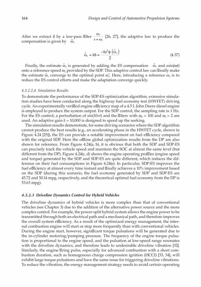
164 Design and Control of Automotive Propulsion Systems
After we extract δ by a low-pass filter ω+ωs
l
l [26, 27], the adaptive law to produce the
compensation is given by ωeˆ
ˆˆ
2
2
kka
ee( )
ω = δ =− φ ω� (4.37)
Finally, the estimate ωeˆ is generated by adding the ES compensation ωeˆ and asin(ωt) onto a reference speed ωe provided by the SDP. This adaptive control law can finally make the estimate ωeˆ converge to the optimal point ω∗
e. Here, introducing a reference ωe is to reduce the ES control efforts and make the adaptation converge quickly.
4.3.2.2.4 Simulation Results
To demonstrate the performance of the SDP-ES optimization algorithm, extensive simula-tion studies have been conducted along the highway fuel economy test (HWFET) driving cycle. An experimentally verified engine efficiency map of a 4.5 L John Deere diesel engine is employed to produce the system output. For the SDP control, the sampling rate is 1 Hz. For the ES control, a perturbation of sin(10πt) and the filters with ωh = 100 and ωl = 2 are used. An adaptive gain k = 10,000 is designed to speed up the seeking.
The simulation results demonstrate, for some driving scenarios where the SDP algorithm cannot produce the best results (e.g., an accelerating phase in the HWFET cycle, shown in Figure 4.24 [25]), the ES can provide a notable improvement on fuel efficiency compared with the original SDP. Here the offline global optimization results from the DP are also shown for reference. From Figure 4.24(a, b), it is obvious that both the SDP and SDP-ES can precisely track the vehicle speed and maintain the SOC at almost the same level (but different from the DP). Figure 4.24(c, d) shows the engine operating profiles (engine speed and torque) generated by the SDP and SDP-ES are quite different, which induces the dif-ference on their fuel consumptions in Figure 4.24(e). In particular, SDP-ES improves the fuel efficiency at almost every time instant and finally achieves a 10% improvement based on the SDP (during this scenario, the fuel economy generated by SDP and SDP-ES are 45.72 and 50.14 mpg, respectively, and the theoretical optimal fuel economy from the DP is 53.63 mpg).
4.3.2.3 Driveline Dynamics Control for Hybrid Vehicles
The driveline dynamics of hybrid vehicles is more complex than that of conventional vehicles (see Chapter 3) due to the addition of the alternative power source and the more complex control. For example, the power-split hybrid system allows the engine power to be transmitted through both an electrical path and a mechanical path, and therefore improves the overall system efficiency. As a result of the optimized energy management, the inter-nal combustion engine will start or stop more frequently than with conventional vehicles. During the engine start, however, significant torque pulsations will be generated due to the in-cylinder motoring/pumping pressure. The frequency of the engine torque pulsa-tion is proportional to the engine speed, and the pulsation at low-speed range resonates with the driveline dynamics, and therefore leads to undesirable driveline vibration [32]. Similarly, the engine firing pulse, especially for advanced combustion with a short com-bustion duration, such as homogenous charge compression ignition (HCCI) [33, 34], will exhibit large torque pulsations and have the same issue for triggering driveline vibrations. To reduce the vibration, the energy management strategy needs to avoid certain operating
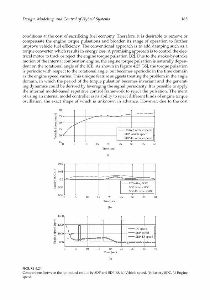
165Design, Modeling, and Control of Hybrid Systems
conditions at the cost of sacrificing fuel economy. Therefore, it is desirable to remove or compensate the engine torque pulsations and broaden its range of operation to further improve vehicle fuel efficiency. The conventional approach is to add damping such as a torque converter, which results in energy loss. A promising approach is to control the elec-trical motor to track or reject the engine torque pulsation [32]. Due to the stroke-by-stroke motion of the internal combustion engine, the engine torque pulsation is naturally depen-dent on the rotational angle of the ICE. As shown in Figure 4.25 [35], the torque pulsation is periodic with respect to the rotational angle, but becomes aperiodic in the time domain as the engine speed varies. This unique feature suggests treating the problem in the angle domain, in which the period of the torque pulsation becomes invariant and the generat-ing dynamics could be derived by leveraging the signal periodicity. It is possible to apply the internal model-based repetitive control framework to reject the pulsation. The merit of using an internal model controller is its ability to reject different kinds of engine torque oscillation, the exact shape of which is unknown in advance. However, due to the cost
0 5 10 15 20 25 30 35 4015
20
25
30
35
40
Time (sec)
Vehi
cle S
peed
(mph
)
Desired vehicle speedSDP vehicle speedSDP-ES vehicle speed
(a)
0 5 10 15 20 25 30 35 400.58
0.59
0.6
0.61
0.62
Time (sec)
Batte
ry S
OC
(1)
DP battery SOCSDP battery SOCSDP-ES battery SOC
(b)
0 5 10 15 20 25 30 35 40
800
1000
1200
1400
Time (sec)
Engi
ne S
peed
(rpm
)
DP speedSDP speedSDP-ES speed
(c)
FIGURE 4.24Comparisons between the optimized results by SDP and SDP-ES. (a) Vehicle speed. (b) Battery SOC. (c) Engine speed.

166 Design and Control of Automotive Propulsion Systems
and accuracy concerns of the sensors, it is desirable to feed back the drive shaft speed oscillation instead of the torque vibration. The vibration of the drive shaft speed has the same frequency feature as the torque vibration, but its amplitude changes continuously. This unique feature again raises the necessity of looking into the tracking control for the periodic but amplitude-varying signal.
0 50 100 150 200 250 300 350 400 450–100
–50
0
50
100
Rotational Angle (deg)(a)
Engi
ne T
orqu
e (N
m)
0 0.1 0.2 0.3 0.4 0.5 0.6 0.7 0.8–100
–50
0
50
100
Time (sec)(b)
Engi
ne T
orqu
e (N
m)
FIGURE 4.25Engine torque oscillation in time and angle domain.
0 5 10 15 20 25 30 35 400
50
100
150
200
Time (sec)
Engi
ne T
orqu
e (N
m) DP torque
SDP torqueSDP-ES torque
(d)
0 5 10 15 20 25 30 35 401
2
3
4
5
6
Time (sec)
Fuel
Con
sum
ptio
n (L
/h)
DP fuel consumptionSDP fuel consumptionSDP-ES fuel consumption
(e)
FIGURE 4.24 (Continued)Comparisons between the optimized results by SDP and SDP-ES. (d) Engine torque. (e) Fuel consumption.
167Design, Modeling, and Control of Hybrid Systems
As revealed in [35], the generating dynamics of the magnitude-varying periodic signal could be time varying, instead of being time invariant, as those for a purely periodic signal. Thus, the traditional repetitive control design, which mainly treats time-invariant generat-ing dynamics, cannot ensure asymptotic tracking performance. Therefore, a new framework for controlling magnitude-varying periodic signals needs to be used. More interestingly, in the hybrid powertrain problem, the magnitude variation for the velocity oscillation to be rejected is due to the integration of the torque vibration with varying frequency, and thus its generating dynamics can be derived. Furthermore, as shown in [35], when the hybrid pow-ertrain vibration problem is treated in the angle domain, the actuator plant dynamics need to be converted to the angle domain as well, which will result in time-varying (actually angle-varying) plant dynamics. Therefore, the time-varying internal model-based control is a good fit for this application. A unique feature of the driveline vibration control for hybrid vehicles is the availability of the alternative power source, such as the motor/generator. By control-ling the motor/generator, it is possible to suppress the driveline vibration and recover the vibration energy into the alternative power. Therefore, it is possible to apply active control to achieve desired driveline dynamics and improve vehicle fuel efficiency at the same time.
References
1. M. Ehsani, Y. Gao, and A. Emani, Modern Electric, Hybrid Electric and Fuel Cell Vehicles, Fundamentals, Theory and Design, 2nd ed., Boca Raton, FL: CRC Press, 2010.
2. A. Sciarretta and L. Guzzella, Control of Hybrid Electric Vehicles, IEEE Control Systems Magazine, 27(2): 60–70, 2007.
3. P. Pisu and G. Rizzoni, A Comparative Study of Supervisory Control Strategies for Hybrid Electric Vehicles, IEEE Transactions on Control Systems Technology, 15(3): 506–518, 2007.
4. C.C. Lin, H. Peng, J.W. Grizzle, and J. Kang, Power Management Strategy for a Parallel Hybrid Electric Truck, IEEE Transactions on Control Systems Technology, 11(6): 839–849, 2003.
5. H. Banvait, S. Anwar, and Y. Chen, “A Rule-Based Energy Management Strategy for Plug-In Hybrid Electric Vehicle (PHEV), in Proceedings of the American Control Conference, St. Louis, MO, 2009, pp. 3938–3943.
6. J. Liu and H. Peng, Modeling and Control of a Power-Split Hybrid Vehicle, IEEE Transactions on Control Systems Technology, 16(6): 1242–1251, 2008.
7. E. Tate, J. Grizzle, and H. Peng, SP-SDP for Fuel Consumption and Tailpipe Emissions Minimization in an EVT Hybrid, IEEE Transactions on Control Systems Technology, 18(3): 673–687, 2010.
8. S. Moura, H. Fathy, D. Callaway, and J. Stein, A Stochastic Optimal Control Approach for Power Management in Plug-In Hybrid Electric Vehicles, IEEE Transactions on Control Systems Technology, 19(3): 545–555, 2011.
9. J. Meyer, K.A. Stelson, A. Alleyne, and T. Deppen, Energy Management Strategy for a Hydraulic Hybrid Vehicle Using Stochastic Dynamic Programming, in Proceedings of the 6th FPNI-PhD Symposium, West Lafayette, IN, 2010, pp. 55–68.
10. C. Musardo, G. Rizzoni, Y. Guezennec, and B. Staccia, A-ECMS: An Adaptive Algorithm for Hybrid Electric Vehicle Energy Management, European Journal of Control, 11: 509–524, 2005.
11. H.A. Borhan, A. Vahidi, A.M. Phillips, M.L. Kuang, and I.V. Kolmanovsky, Predictive Energy Management of a Power-Split Hybrid Electric Vehicle, in Proceedings of the American Control Conference, St. Louis, MO, 2009, pp. 3970–3976.
12. T. Deppen, A. Alleyen, K.A. Stelson, and J. Meyer, A Model Predictive Control Approach for a Parallel Hydraulic Hybrid Powertrain, in Proceedings of the American Control Conference, San Francisco, CA, 2011, pp. 2713–2718.

168 Design and Control of Automotive Propulsion Systems
13. C.D. Rakopoulos and E.G. Giakoumis, Diesel Engine Transient Operation, London: Springer, 2009.
14. J.R. Hagena, Z. Filipi, and D.N. Assanis, Transient Diesel Emissions: Analysis of Engine Operation during a Tip-In, SAE Technical Paper 2006-01-1151, 2006.
15. Y. Wang, H. Zhang, and Z. Sun, Optimal Control of the Transient Emissions and the Fuel Efficiency of a Diesel Hybrid Electric Vehicle, Journal of Automobile Engineering, 227(11): 1546–1561, 2013.
16. M. Benz, C.H. Onder, and L. Guzzella, Engine Emission Modeling Using a Mixed Physics and Regression Approach, Journal of Engineering for Gas Turbines and Power, 132(4): 042803, 2010.
17. Y. Wang, Y. He, and S. Rajagopalan, Design of Engine-Out Virtual NOx Sensor Using Neural Networks and Dynamic System Identification, SAE International Journal of Engines, 4(1): 837–849, 2011.
18. C. Ericson and B. Westerberg, Transient Emission Prediction with Quasi Stationary Models, SAE Technical Paper 2005-01-3852, 2005.
19. R. Ahlawat, J.R. Hagena, Z.S. Filipi, J.L. Stein, and H.K. Fathy, Volterra Series Estimation of Transient Soot Emissions from a Diesel Engine, in IEEE Vehicle Power and Propulsion Conference (VPPC), Lille, France, 2010, pp. 1–7.
20. M. Adlouni, Modeling of Soot Emission for Heavy-Duty Diesel Engines in Transient Operation, Master’s thesis, Lund University, Sweden, 2011.
21. E. Eskinat, S. Johnson, and W. Luyben, Use of Hammerstein Models in Identification of Nonlinear Systems, AlChE Journal, 37(2): 255–268, 1991.
22. D. Kirk, Optimal Control Theory: An Introduction, Upper Saddle River, NJ: Prentice Hall, 1970. 23. Y. Wang and Z. Sun, A Hydrostatic Dynamometer Based Hybrid Powertrain Research Platform,
in Proceedings of the International Symposium on Flexible Automation, Tokyo, Japan, 2010, UPS-2739. 24. Y. Wang, Z. Sun, and K.A. Stelson, Modeling, Control and Experimental Validation of a
Transient Hydrostatic Dynamometer, IEEE Transactions on Control Systems Technology, 19(6): 1578–1586, 2011.
25. Y. Wang and Z. Sun, SDP-Based Extremum Seeking Energy Management Strategy for a Power-Split Hybrid Electric Vehicle, in Proceedings of the American Control Conference, Montreal, Canada, 2012, pp. 553–558.
26. K. Ariyur and M. Krstic, Real Time Optimization by Extremum Seeking Control, New York: John Wiley & Sons, 2003, pp. 3–20.
27. M. Krstic and H. Wang, Stability of Extremum Seeking Feedback for General Nonlinear Dynamic Systems, Automatica, 36(2000): 595–601, 2000.
28. L. Serrao, S. Onori, and G. Rizzoni, ECMS as a Realization of Pontryagin’s Minimum Principle for HEV Control, in Proceedings of the American Control Conference, St. Louis, MO, 2009, pp. 3964–3969.
29. P.Y. Li and F. Mensing, Optimization and Control of a Hydro-Mechanical Transmission Based Hybrid Hydraulic Passenger Vehicle, presented at Proceedings of the 7th International Fluid Power Conference, Aachen, Germany, 2010.
30. C.T. Li and H. Peng, Optimal Configuration Design for Hydraulic Split Hybrid Vehicles, in Proceedings of the American Control Conference, Baltimore, MD, 2010, pp. 5812–5817.
31. Y. Wang, X. Song, and Z. Sun, Hybrid Powertrain Control with a Rapid Prototyping Research Platform, in Proceedings of the American Control Conference, San Francisco, CA, 2011, pp. 997–1002.
32. S. Tomura, Y. Ito, K. Kamichi, and A. Yamanaka, Development of Vibration Reduction Motor Control for Series-Parallel Hybrid System, SAE Technical Paper 2006-01-1125, 2006.
33. T. Kuo, Valve and Fueling Strategy for Operating a Controlled Auto-Ignition Combustion Engine, in SAE Homogeneous Charge Compression Ignition Symposium, San Ramon, CA, 2006, pp. 11–24.
34. T. Kuo, Z. Sun, J. Eng, B. Brown, P. Najt, J. Kang, C. Chang, and M. Chang, Method of HCCI and SI Combustion Control for a Direct Injection Internal Combustion Engine, U.S. Patent 7,275,514, 2007.
35. X. Song, P. Gillella, and Z. Sun, Tracking Control of Periodic Signals with Varying Magnitude and Its Application to Hybrid Powertrain, in Proceedings of the ASME Dynamic Systems and Control Conference, Cambridge, MA, 2011, DSCC2010-4189.
169
5Control System Integration and Implementation
5.1 Introduction to the Electronic Control Unit
An electronic control unit (ECU), also called the powertrain control module (PCM), is a type of electronic controller equipped with one or a few microprocessors that control a series of engine or transmission actuators based upon the sensor feedbacks to ensure the optimal engine or transmission performance. Before the electronic control became available, the engine air-to-fuel ratio, ignition timing, and idle speed were dynamically controlled by mechanical and pneumatic means.
5.1.1 Electronic Control Unit (ECU)
Modern ECUs use one or multiple microprocessor cores to process the inputs from the engine sensors and generate the corresponding control outputs for actuators in real time. An electronic control unit contains both the hardware and software. The hardware consists of electronic components on a printed circuit board (PCB), ceramic substrate, or thin lami-nate substrate. The main component on this circuit board is one or a few microcontrollers (CPUs). The software is often stored in the microcontroller(s) or other memory chips on the PCB, typically in so-called erasable programmable read-only memories (EPROMs) or flash memory so the CPU can be reprogrammed by uploading updated code or replacing chips. The engine control system is also called an (electronic) engine management system (EMS). Figure 5.1 shows a sample ECU architecture, with the sensors and actuators in the dotted boxes.
Besides managing the engine combustion process, a modern engine management system also controls many engine subsystems, such as variable valve timing subsystem, electronic throttle, exhaust gas recirculation (EGR) system, turbocharger and wastegate subsystems, and so on. The ECU also communicates with other control units, such as the transmission control unit and traction control unit, through the control area network (CAN).
5.1.1.1 ECU Control Features
There are many control features for an engine control system, including air-to-fuel ratio control, engine ignition timing control, EGR control, engine valve timing control, etc. The following is a list of these key control features.
1. Air-to-fuel ratio control. The engine air-to-fuel ratio is normally controlled by the injected fuel quantity, where engine load (or output torque) is normally con-trolled by the engine throttle (or charge air). Since the three-way catalyst provides

170 Design and Control of Automotive Propulsion Systems
the highest conversion efficiency for hydrocarbon (HC), carbon monoxide (CO), and nitrogen oxides (NOx) at the stoichiometric air-to-fuel ratio (see Figure 5.2), in order to minimize the tailpipe emissions the gasoline engine needs to be operated at its air-to-fuel ratio close to the stoichiometric level, which is the main motivation for the air-to-fuel ratio regulation. The electronic control unit (ECU) determines the quantity of fuel to be injected based upon a number of parameters, such as acceleration pedal position, engine coolant temperature, engine speed, and so on. For the port fuel injection (PFI) fuel system, the transient air-to-fuel ratio control will be fairly challenging due to the so-called wall-wetting dynamics. Advanced control technology can be used to improve the accuracy of the air-to-fuel control during transient operations; see references [1–3].
2. Ignition (spark) timing control. A spark-ignited (SI) engine requires a spark to ini-tiate the in-cylinder combustion process. An ECU adjusts the spark timing (or ignition timing) to optimize engine fuel economy with satisfactory emissions and improved power output. That is, if possible, the engine shall be operated at its maximum torque for the best torque (MBT) timing for the best fuel economy. As the result of engine downsizing, turbocharged engines are becoming popu-lar and engine knock control becomes even more important. Besides engine EGR control, engine ignition timing is often used to control the engine knock; see ref-erences [4–6]. Since engine cold-start emissions consist of up to 80% of the total emissions of the Federal Test Procedure (FTP) driving cycle, reducing cold-start duration is very important for the SI engines. The spark timing is often retarded during the cold start to increase the exhaust temperature so that the three-way
Appl
icat
ion
Code
Dia
gnos
tics
Code
Ope
ratin
gSy
stem
Inpu
t Dev
ice
Out
put D
evic
e
MCU Reset
SPI SCI/CAN
Voltage Regulation Harshness Protection
MCU ResetControl
FuelInjectorDriver
IgnitionCoil
Driver
SolenoidDriver
SolenoidDriver
DiagnosticBus Driver
Fuel Injector
Fuel Injector
…
Ignition Coil
Ignition Coil
…
EGR valve
Idle Spd Valve
Diagnostic Bus
Output Devices
InputSignal
Conditioning
Ampli�er
ProtocolDevices
Crank Position
Analog Input
Analog Output
Vehicle Speed
Engine Temp
Ambient Temp
Fuel Pressure
MAP ABS
�rottle Position
Mass Air Flow
Knock Sensor
O2 Sensor
O2 Sensor
Oil Pressure
• • •
Battery
FIGURE 5.1ECU architecture with sensors and actuators.

171Control System Integration and Implementation
catalyst can be warmed up quickly. However, heavily retarded spark timing could lead to unstable combustion [4], and closed-loop control of the spark tim-ing makes it possible to operate the engine at its maximum allowed retard timing with guaranteed combustion stability.
3. Idle speed control. Idle speed control is often part of the modern engine control system. The engine speed is measured by the so-called crankshaft position sensor, which also provides real-time engine position information for generating engine position-related control signals, such as ignition timing control, fuel injection con-trol, and direct injection (DI) fuel pump control. Idle speed is controlled by an idle air bypass control stepper motor or a linear solenoid, while the engine throttle is positioned at its default limp-home position. The idle speed control must be robust to various engine load changes, such as air conditioning compressor or transmis-sion engagement torque loads. Note that a full authority throttle control system can also be used to control engine idle speed and manage high-speed limitations.
4. Variable valve timing (VVT) control. To improve the engine fuel economy, most modern engines are equipped with VVT actuators to make it possible to adjust the engine intake or exhaust valve timings to their optimal positions for the best fuel economy. There are two kinds of VVT actuators: electrohydraulic and electric VVT. Both actuators regulate the relative position between the crank- and camshafts such that the intake or exhaust timing can be controlled. This feature can be used to optimize the charge airflow into the cylinder for the best fuel economy. The control of the electrohydraulic VVT [8] is through a proportional solenoid valve, and the control of the electric VVT [7] is by regulating the ring gear speed of the electric VVT planetary gear set through the electric motor. A cam position sensor is often used for closed-loop control.
5. Exhaust gas recirculation (EGR) control. The engine EGR is often used to reduce the engine NOx emissions, and recently it was also used to suppress the engine knock. Since a high EGR rate could lead to unstable combustion, to maxi-mize the percentage of emission reduction, the EGR rate needs to be controlled in a closed loop to maintain the combustion stability [9]. The EGR rate is often controlled through an EGR valve driven by either a DC or step motor. A delta
Con
vers
ion
E�ci
ency
%
100
80HC
CO
NOx
λ1.110.9
60
40
20
FIGURE 5.2Conversion efficiencies of the three-way catalyst.
172 Design and Control of Automotive Propulsion Systems
pressure sensor is often used to estimate the EGR flow rate for closed-loop control. For the engine equipped with the turbocharger, the EGR can also be controlled by regulating the exhaust pressure through the variable geometry turbocharger or wastegate.
6. Variable geometry turbocharger and wastegate control. The turbocharger is used to boost intake manifold pressure to increase the engine power density and improve fuel economy. A variable geometry turbocharger is used to alter the turbo-map to best match the engine operational condition undercurrent speed and load condition. The wastegate is often used, along with the variable geometry turbocharger, to regulate the boost and exhaust pressures.
5.1.2 Communications between ECUs
Bosch originally developed the control area network (CAN) in 1985 for in-vehicle networks. Before that, automotive manufacturers connected electronic devices in vehicles using point-to-point wiring systems. As the number of electronic control devices increased, the wire harness got bulky, heavy, and expensive. It was then replaced by in-vehicle networks such as CAN to reduce wiring cost, complexity, and weight. CAN, a high-integrity serial bus system for networking intelligent devices, became the standard in-vehicle network. The automotive industry quickly adopted CAN, and in 1993, it became the international standard known as ISO 11898.
The main benefits of using CAN are the low cost and light weight. That is, the CAN network provides a low-cost, durable, and reliable network that enables communication among multiple CAN devices. The main advantage of CAN communication is that elec-tronic control units (ECUs) can have a single CAN interface rather than using multiple wires to connect the analog and digital signals between these control units. This decreases overall cost and weight in automobiles. The following is a list of CAN communication features:
1. Communication broadcast. Each of the devices on the network has a CAN con-troller chip. All devices on the CAN network see all transmitted messages. Each device can decide if a message is relevant to itself. If not, it will be filtered. This structure allows modifications to CAN networks with minimal impact, and addi-tional nontransmitting nodes can be added without modification to the network.
2. Priority. Each CAN message has a priority assigned such that if two nodes try to send messages simultaneously, the node with the higher priority has the right of transmission and the node with the lower priority gets postponed. This arbitration is nondestructive and results in noninterrupted transmission of the highest priority message. This also allows networks to meet deterministic timing constraints.
3. Error capability. The CAN specification includes a cyclic redundancy code (CRC) to perform error checking on the contents of each frame. Frames with errors are disregarded by all nodes, and an error frame can be transmitted to signal the error to the network. Global and local errors are differentiated by the controller, and if too many errors are detected, individual nodes can stop transmitting errors or disconnect themselves from the network completely.
4. CAN physical layers. CAN has several different physical layers you can use. These physical layers classify certain aspects of the CAN network, such as electrical

173Control System Integration and Implementation
levels, signaling schemes, cable impedance, maximum baud rates, and more. The most common and widely used physical layers are described below:• High-speed CAN is by far the most common physical layer. High-speed CAN
networks are implemented with two wires and allow communication at trans-fer rates up to 1 Mbit/s. Other names for high-speed CAN include CAN C and ISO 11898-2. Typical high-speed CAN devices include antilock brake systems, engine control modules, transmission control systems, and emission systems.
• Low-speed/fault-tolerant CAN networks are also implemented with two wires, can communicate with devices at rates up to 125 Kbit/s, and offer transceivers with fault-tolerant capabilities. Other names for low-speed/fault-tolerant CAN include CAN B and ISO 11898-3. Typical low-speed/fault-tolerant devices in an automobile include comfort devices. Wires that have to pass through the door of a vehicle are low speed/fault tolerant in light of the stress that is inherent to opening and closing a door. Also, in situations where an advanced level of security is desired, such as with brake lights, low-speed/fault-tolerant CAN offers a solution.
• Single-wire CAN interfaces can communicate with devices at rates up to 33.3 Kbit/s (88.3 Kbit/s in high-speed mode). Other names for single-wire CAN include SAE-J2411, CAN A, and GMLAN. Typical single-wire devices within an automobile do not require high performance. Common applications include comfort devices such as seat and mirror adjusters.
• Software-selectable CAN hardware, such as National Instruments CAN hardware products, can be configured by software to select the desired CAN interface for the onboard transceivers among the high-speed, low-speed/fault-tolerant, and single-wire CANs. Multiple-transceiver hardware offers the perfect solu-tion for applications that require a combination of communications standards.
CAN was first created for automotive applications. Therefore, the most common application is in-vehicle electronic networking. However, as other industries have real-ized the dependability and advantages of CAN communication over the past decades, it has been adopted in various applications. For example, the railway applications include different levels of the multiple networks, such as linking the door units or brake con-trollers, passenger counting units, and more. CAN also has applications in aircraft with flight state sensors, navigation systems, and so on. In addition, you can find CAN buses in many aerospace applications, ranging from in-flight data analysis to aircraft engine con-trol systems such as fuel systems, pumps, and linear actuators.
The medical equipment industry also uses CAN as an embedded network in medical devices. Some hospitals use CAN to manage complete operating rooms, including control of the operating room components such as lights, tables, cameras, x-ray machines, and patient beds.
5.1.3 Calibration Methods for ECU
The engine and powertrain calibration process is always associated with high cost and long duration due to the system complexity. To determine the optimal powertrain and engine control parameters with respect to the desired performance, fuel economy, and emissions, the characteristics of the powertrain and engine system need to be accurately measured. Due to the high degrees of system freedom, a complete mapping is extremely
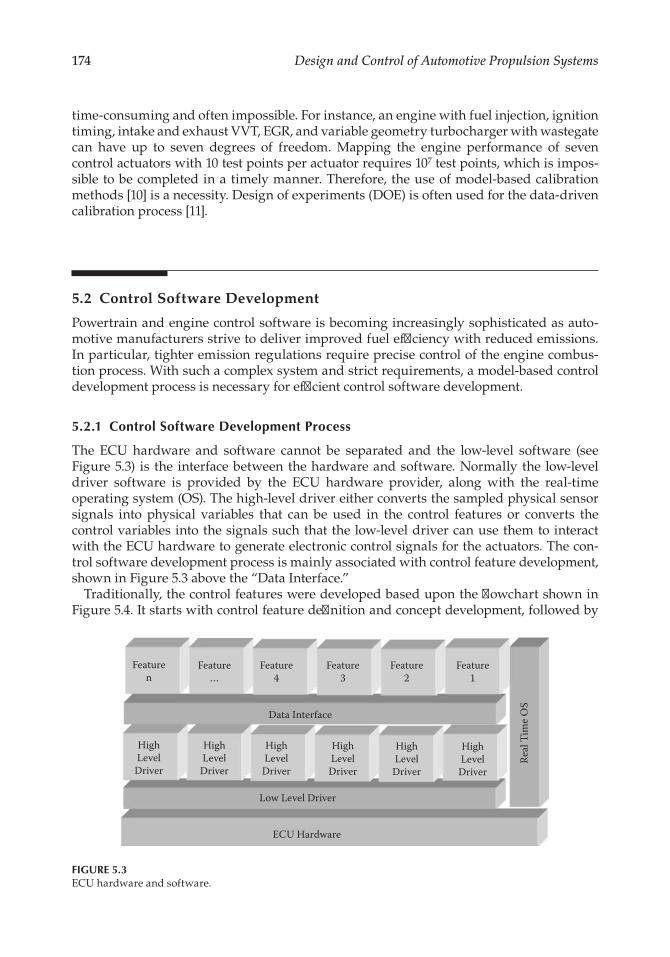
174 Design and Control of Automotive Propulsion Systems
time-consuming and often impossible. For instance, an engine with fuel injection, ignition timing, intake and exhaust VVT, EGR, and variable geometry turbocharger with wastegate can have up to seven degrees of freedom. Mapping the engine performance of seven control actuators with 10 test points per actuator requires 107 test points, which is impos-sible to be completed in a timely manner. Therefore, the use of model-based calibration methods [10] is a necessity. Design of experiments (DOE) is often used for the data-driven calibration process [11].
5.2 Control Software Development
Powertrain and engine control software is becoming increasingly sophisticated as auto-motive manufacturers strive to deliver improved fuel efficiency with reduced emissions. In particular, tighter emission regulations require precise control of the engine combus-tion process. With such a complex system and strict requirements, a model-based control development process is necessary for efficient control software development.
5.2.1 Control Software Development Process
The ECU hardware and software cannot be separated and the low-level software (see Figure 5.3) is the interface between the hardware and software. Normally the low-level driver software is provided by the ECU hardware provider, along with the real-time operating system (OS). The high-level driver either converts the sampled physical sensor signals into physical variables that can be used in the control features or converts the control variables into the signals such that the low-level driver can use them to interact with the ECU hardware to generate electronic control signals for the actuators. The con-trol software development process is mainly associated with control feature development, shown in Figure 5.3 above the “Data Interface.”
Traditionally, the control features were developed based upon the flowchart shown in Figure 5.4. It starts with control feature definition and concept development, followed by
ECU Hardware
Low Level Driver
HighLevel
Driver
HighLevel
Driver
HighLevel
Driver
HighLevel
Driver
HighLevel
Driver
HighLevel
Driver
Feature1
Feature2
Feature3
Feature4
Feature…
Featuren
Real
Tim
e OS
Data Interface
FIGURE 5.3ECU hardware and software.

175Control System Integration and Implementation
an iterative process of vehicle and dynamometer tests, software specification development and implementation, and software integration and testing. This process may iterate a few times until the software is ready for release. This is a fairly lengthy process since each iter-ation involves vehicle and dynamometer tests with manual software programming and implementation. Also, since it is a manual process, there is no mechanism to guarantee that the developed software will be consistent with the initial concept, and manual soft-ware debugging is also a concern. Therefore, the control feature development is moving toward a model-based process, as shown in Figure 5.5.
The model-based software development process is demonstrated in Figure 5.5, where the vehicle and dynamometer tests are replaced by simulations based upon the real-time (or control-oriented) engine model described in Chapter 2. During the con-trol feature development process, the feature requirement will be documented by the graphical Simulink model, and the control feature is also developed and validated in
FeatureConcept
Development �roughVehicle/Dyno Testing
SoftwareSpeci�cations
SoftwareImplementation
SoftwareIntegration & Testing
Software Release to Calibration
FIGURE 5.4Traditional control feature development process.
Feature Designand De�nition`
Software DevelopmentAutocode Generation
Graphical Models
CIL/HIL Simulation
Calibration/Validation
Rapid Prototyping DevModeling & SimulationAutocode Generation
FeatureConceptual Design
SimulinkModeling
Testing andParameter Tuning
Automatic CodeGeneration
Calibration Guidelines
FIGURE 5.5Rapid prototype (model-based) control development.

176 Design and Control of Automotive Propulsion Systems
a Simulink environment. Note that in order to validate the developed control feature, a control- oriented engine model (described in Chapter 2) is required. One of the features of this model-based development process is that the initial control feature calibrations can be generated during the feature validation process. Also, software autocode generation is part of the process that will be discussed in the next subsection.
Controller-in-the-loop (CIL) and hardware-in-the-loop (HIL) simulations are the key for validating the control features developed by the model-based process. The CIL simula-tions are conducted with a production ECU and an engine simulator, where the developed control feature is implemented into the production ECU. This is an important step since it validates the fact that the developed control feature can be executed in the produc-tion ECU, while the HIL simulation environment consists of the production ECU and a hybrid engine simulation platform that comprises a real-time simulator and part of the engine hardware, such as fuel injectors, ignition coils, etc. Therefore, CIL simulation is a special case of the HIL simulation, where no engine hardware is used in the simulation environment.
5.2.2 Automatic Code Generation
After the developed control feature has been validated to meet the specifications and requirements through software-in-the-loop (SIL) simulations (see Figure 5.5), the next step is to develop the software that can be deployed into the target ECU or an embedded processor. Since the control feature is developed in a MATLAB®/Simulink® environment, it is natural to use the MathWorks’ Real-Time Workshop Embedded Coder (or Simulink Coder) to automatically generate highly efficient C/C++ code from the feature control model in Simulink. The code generated by the Embedded Coder is capable of running on virtually any microprocessor or real-time operating system (RTOS). The generated code can also be integrated back into Simulink for SIL simulation validation, and then deployed directly to a supported microprocessor for CIL and HIL simulation validation.
The main advantage of the autocode generation is its traceability among the Simulink-based feature requirements (specifications), the feature control model, feature test vectors used to validate the developed feature, and the C/C++ code generated by the Embedded Coder. This ensures that any design decision (selection) made earlier in the feature devel-opment process is fully documented within the generated code. The ability to navigate from the Simulink feature definition to the developed control feature in Simulink and to the embedded C/C++ code generated by Simulink Coder provides a systematic approach for control software development. It is common in the automotive industry that the control feature requirements need to be changed to meet future fuel economy and emis-sion requirements. With the model-based development process, the modifications can be made in the Simulink-based control feature and the modified feature can be validated through the software-in-the-loop (SIL) simulations. After the feature is validated in SIL simulations, the code generation can be done automatically, which reduces the feature modification duration significantly, and hence reduces software development cost.
5.2.3 Software-in-the-Loop (SIL) Simulation
There are many definitions for SIL simulations. In this book, we call the co-simulation conducted on a single computer platform with both engine model and its controller the SIL simulation (see Figure 5.6). It can be divided into two main categories: model-in-the-loop (MIL) simulation and software-in-the-loop simulation. MIL simulations use a controller

177Control System Integration and Implementation
model (normally in Simulink) along with a plant (engine) model, and the control model is connected directly to a physical model of the system within the same Simulink diagram. In this case, any small modifications to the control model can be immediately tested in the MIL simulation environment, and it is also very easy to tune the control parameters with simulation validation so that the initial calibrations can be generated in this stage. The SIL simulation environment makes the simulation more realistic by replacing the Simulink-based control strategy with the strategy based upon the embedded C/C++ code. This type of simulation can be used to check if there is any difference between the Simulink-based and embedded code-based strategies by running the parallel simulations with both con-trollers at the same time. The SIL simulation is closer to the actual implementation since the target-embedded C/C++ code is executed in the simulations, which is essential for validating the coding system (whether autocoded or human coded).
5.2.4 Hardware-in-the-Loop (HIL) Simulation
As discussed before, the HIL simulation environment consists of the engine control model, engine model simulator, and engine system-associated hardware. This subsection con-centrates on the controller-in-the-loop (CIL) simulations as shown in Figure 5.7, where an Opal-RT-based engine prototype controller was used to control the virtual engine simulated by a dSPACE simulator in a CIL simulation environment. In the rest of this subsection the charge air control feature of a homogeneous charge compression ignition (HCCI) engine is used to demonstrate the rapid prototype control development process discussed in this chapter.
5.2.4.1 HCCI Combustion Background
Homogeneous charge compression ignition (HCCI) combustion has the potential for internal combustion (IC) engines to meet the increasingly stringent emissions regula-tions with improved fuel economy [12]. The flameless nature of the HCCI combustion and its high dilution operation capability lead to low combustion temperature. As a result, the formation of NOx can be significantly reduced [13]. Furthermore, the HCCI engine is capable of unthrottled operation that greatly reduces pumping loss and improves fuel economy [14, 15].
On the other hand, the HCCI combustion has its own limitations. It is limited at high engine load due to the mechanical limit, and at low load due to misfire caused by the lack
Control-OrientedEngineModel
Engi
ne C
ontr
ol A
lgor
ithm
s
Cont
rol
Feat
ure t
o Be
Valid
ated
Actuator Signals
Sensor Signals
FIGURE 5.6SIL simulation environment.
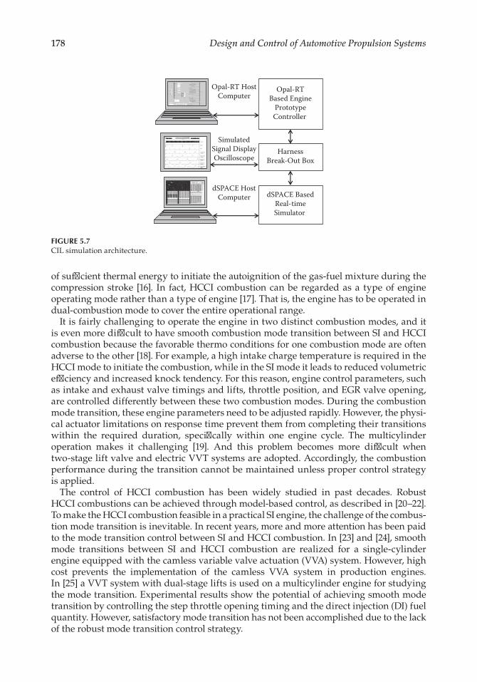
178 Design and Control of Automotive Propulsion Systems
of sufficient thermal energy to initiate the autoignition of the gas-fuel mixture during the compression stroke [16]. In fact, HCCI combustion can be regarded as a type of engine operating mode rather than a type of engine [17]. That is, the engine has to be operated in dual-combustion mode to cover the entire operational range.
It is fairly challenging to operate the engine in two distinct combustion modes, and it is even more difficult to have smooth combustion mode transition between SI and HCCI combustion because the favorable thermo conditions for one combustion mode are often adverse to the other [18]. For example, a high intake charge temperature is required in the HCCI mode to initiate the combustion, while in the SI mode it leads to reduced volumetric efficiency and increased knock tendency. For this reason, engine control parameters, such as intake and exhaust valve timings and lifts, throttle position, and EGR valve opening, are controlled differently between these two combustion modes. During the combustion mode transition, these engine parameters need to be adjusted rapidly. However, the physi-cal actuator limitations on response time prevent them from completing their transitions within the required duration, specifically within one engine cycle. The multicylinder operation makes it challenging [19]. And this problem becomes more difficult when two-stage lift valve and electric VVT systems are adopted. Accordingly, the combustion performance during the transition cannot be maintained unless proper control strategy is applied.
The control of HCCI combustion has been widely studied in past decades. Robust HCCI combustions can be achieved through model-based control, as described in [20–22]. To make the HCCI combustion feasible in a practical SI engine, the challenge of the combus-tion mode transition is inevitable. In recent years, more and more attention has been paid to the mode transition control between SI and HCCI combustion. In [23] and [24], smooth mode transitions between SI and HCCI combustion are realized for a single- cylinder engine equipped with the camless variable valve actuation (VVA) system. However, high cost prevents the implementation of the camless VVA system in production engines. In [25] a VVT system with dual-stage lifts is used on a multicylinder engine for studying the mode transition. Experimental results show the potential of achieving smooth mode transition by controlling the step throttle opening timing and the direct injection (DI) fuel quantity. However, satisfactory mode transition has not been accomplished due to the lack of the robust mode transition control strategy.
dSPACE BasedReal-timeSimulator
HarnessBreak-Out Box
Opal-RTBased Engine
PrototypeController
dSPACE HostComputer
Opal-RT HostComputer
SimulatedSignal DisplayOscilloscope
FIGURE 5.7CIL simulation architecture.

179Control System Integration and Implementation
The controller-in-the-loop (CIL) simulation results, shown below, demonstrated that unstable combustion during the transition can be eliminated by using the multistep strat-egy as discussed in [26] for a four-cylinder engine equipped with external cooled EGR, dual-stage valve lift, and electrical VVT system. The rest of this section utilizes the linear quadratic (LQ) optimal manifold air pressure (MAP) tracking control strategy to main-tain the air-to-fuel ratio in the desired range so that hybrid (or spark-assisted) combustion is feasible. Under the optimal MAP control, smooth combustion mode transition can be achieved with the help of the iterative learning control (ILC) of the DI fuel quantity of indi-vidual cylinders. Note that the ILC is mainly used to generate transient fuel calibrations. The entire control strategy was validated in the CIL engine simulation environment [27], and satisfactory engine performance was achieved during the combustion mode transi-tion for both steady-state and transient operating conditions.
5.2.4.2 Multistep Combustion Mode Transition Strategy
The configuration of the target HCCI-capable SI engine and the engine specifications are listed in Table 5.1. The key feature of this engine is its valvetrain system. It has two-stage lift for both intake and exhaust valves. The high lift has 9 mm maximum lift for the SI com-bustion mode, and the low lift has 5 mm maximum lift for the HCCI combustion mode. The ranges of both intake and exhaust valve timing are extended to ±40 crank degrees to improve the controllability of the internal EGR fraction, the effective compression ratio, and the engine volumetric efficiency during the combustion mode transition and HCCI operations. The externally cooled EGR is used to enable high dilution charge with a low charge mixture temperature.
For this application example, the combustion mode transition was studied for the engine operated at 2000 rpm with 4.5 bar indicated mean effective pressure (IMEP). Table 5.2 lists the engine parameters associated with the SI and HCCI combustion. These parameters were optimized for steady-state engine operation with the best fuel economy that satisfies the engine knock limit requirement. It can be seen in Table 5.2 that the optimized engine control parameters are quite different between the SI and HCCI combustion modes. Some of these parameters can be adjusted within one engine cycle, such as spark timing θST, electronic throttle control (ETC) drive current IETC that is proportional to throttle motor torque, DI fuel quantity FDI, and valve lift Πlift; the others cannot due to slow actuator dynamics.
The combustion characteristics are also quite different between these two combustion modes, as illustrated in Figure 5.8. For example, the HCCI combustion has higher peak
TABLE 5.1
HCCI-Capable SI Engine Specifications
Engine Parameter Model Value
Bore/stroke/con-rod length 86 mm/86 mm/143.6 mmCompression ratio 9.8:1Intake/exhaust valve lifts of high stage 9 mm/9 mmIntake/exhaust valve lifts of low stage 5 mm/5 mmIntake/exhaust valve timing range ±40°/±40°Intake/exhaust valve lifts lash 0.2 mm/0.25 mmIntake manifold volume 3.2 LThrottle diameter 42 mm
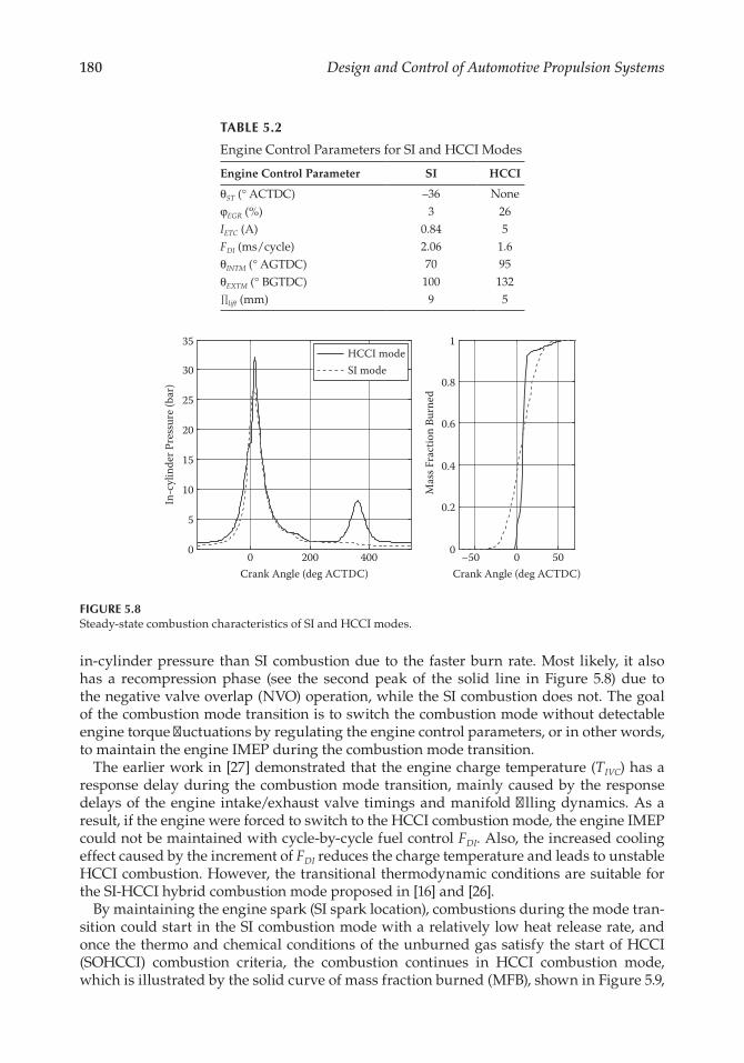
180 Design and Control of Automotive Propulsion Systems
in-cylinder pressure than SI combustion due to the faster burn rate. Most likely, it also has a recompression phase (see the second peak of the solid line in Figure 5.8) due to the negative valve overlap (NVO) operation, while the SI combustion does not. The goal of the combustion mode transition is to switch the combustion mode without detectable engine torque fluctuations by regulating the engine control parameters, or in other words, to maintain the engine IMEP during the combustion mode transition.
The earlier work in [27] demonstrated that the engine charge temperature (TIVC) has a response delay during the combustion mode transition, mainly caused by the response delays of the engine intake/exhaust valve timings and manifold filling dynamics. As a result, if the engine were forced to switch to the HCCI combustion mode, the engine IMEP could not be maintained with cycle-by-cycle fuel control FDI. Also, the increased cooling effect caused by the increment of FDI reduces the charge temperature and leads to unstable HCCI combustion. However, the transitional thermodynamic conditions are suitable for the SI-HCCI hybrid combustion mode proposed in [16] and [26].
By maintaining the engine spark (SI spark location), combustions during the mode tran-sition could start in the SI combustion mode with a relatively low heat release rate, and once the thermo and chemical conditions of the unburned gas satisfy the start of HCCI (SOHCCI) combustion criteria, the combustion continues in HCCI combustion mode, which is illustrated by the solid curve of mass fraction burned (MFB), shown in Figure 5.9,
0 200 4000
5
10
15
20
25
30
35
Crank Angle (deg ACTDC)
In-c
ylin
der P
ress
ure (
bar)
–50 0 500
0.2
0.4
0.6
0.8
1
Crank Angle (deg ACTDC)
Mas
s Fra
ctio
n Bu
rned
HCCI modeSI mode
FIGURE 5.8Steady-state combustion characteristics of SI and HCCI modes.
TABLE 5.2
Engine Control Parameters for SI and HCCI Modes
Engine Control Parameter SI HCCI
θST (° ACTDC) –36 None
φEGR (%) 3 26IETC (A) 0.84 5FDI (ms/cycle) 2.06 1.6θINTM (° AGTDC) 70 95
θEXTM (° BGTDC) 100 132Πlift (mm) 9 5

181Control System Integration and Implementation
obtained through GT-Power simulations. During an ideal SI-to-HCCI combustion tran-sition process, the HCCI combustion percentage (the vertical distance from SOHCCI to MFB = 1) increases gradually along with the gradual increase of charge temperature (TIVC). For the HCCI-to-SI combustion transition, the HCCI combustion percentage will be gradu-ally reduced. More importantly, during the SI-HCCI hybrid combustion, engine IMEP can be controlled by regulating the DI fuel quantity, which will be discussed later. This is the other motivation for utilizing the hybrid combustion mode during the combustion mode transition.
In [26], a crank-based SI-HCCI hybrid combustion model was developed for real-time control strategy development. It models the SI combustion phase under the two-zone assumption and the HCCI combustion phase under the one-zone assump-tion. The SI and HCCI combustion modes are actually special cases of the SI-HCCI hybrid combustion mode in the model, since the SI combustion occurs when the HCCI combustion does not occur, and the HCCI combustion occurs when the percentage is 100%. Accordingly, this combustion model is applicable for all combustion modes during the mode transition.
In [27], the one-step combustion mode transition was investigated. The control references of all engine parameters were directly switched from the SI mode to HCCI mode, as listed in Table 5.2, in one engine cycle. The simulation results showed that misfires occur during the one-step mode transition, and significant torque fluctuation was discovered. Thereby, a multistep mode transition strategy was proposed in [27] by inserting a few hybrid com-bustion cycles between the SI and HCCI combustion (see Figure 5.10). The proposed con-trol strategy is based on this multistep strategy.
As illustrated in Figure 5.10, five engine cycles are used during the SI-to-HCCI mode transition. During the transitional cycles, some engine parameters are adjusted in open loop according to the schedule shown in Figure 5.10. Cycles 1 and 2 are used for engine throttle control. They provide enough time for the engine MAP to increase to compensate the valve lift (Πlift) switch. At the end of cycle 2, the intake/exhaust valve lift Πlift switches from high lift to low lift, and the control references of EGR fraction φEGR, intake valve timing θINTM, and exhaust valve timing θEXTM are set to those of the steady-state HCCI com-bustion mode as listed in Table 5.2. Spark timing θST of each cylinder was kept constant
–80 –60 –40 –20 0 20 40 60 80
0
0.2
0.4
0.6
0.8
1
Crank Angle (deg)
Mas
s Fra
ctio
n Bu
rned
SI-HCCI hybrid modeHCCI modeSI mode
ST
SOHCCI
FIGURE 5.9MFB trace of SI-HCCI hybrid combustion mode.

182 Design and Control of Automotive Propulsion Systems
during the transitional cycles and was eliminated at the end of cycle 5. Throughout the transitional cycles, the engine control parameters, throttle current IETC, and DI fueling FDI are regulated with the time-based control at a sample period of 1 ms and with cycle-based controls, respectively.
5.2.4.3 Air-to-Fuel Ratio Tracking Problem
To study the feasibility of using fuel injection quantity FDI to regulate the engine IMEP, intensive simulations were conducted to map out the engine IMEP and air-to-fuel ratio as functions of engine fuel injection quantity FDI and manifold air pressure (MAP). The simu-lation results are shown in Figure 5.11, indicating that the engine IMEP is highly correlated to FDI with the lean air-to-fuel mixture. As a result, it is possible to control the individual cylinder IMEP by regulating the corresponding FDI.
To maintain the controllability of the DI fueling (FDI), a lean gas-fuel mixture is required during the mode transition. However, the combustion could become unstable if the mix-ture becomes extremely lean since the engine spark might not be able to ignite the gas mixture. For this study, the desired normalized air-to-fuel ratio is set between λmin (0.97) and λmax (1.3). In [27], a step throttle preopening approach was proposed to prevent rich combustions at cycle 3, but it leads to very lean combustion in the following engine cycles. For this application, an LQ tracking control strategy [28] is developed to regulate the air-to-fuel ratio around the desired level.
As discussed above, the normalized air-to-fuel ratio needs to be maintained within the optimal range (λmin ≤ λ ≤ λmax) during the SI-to-HCCI combustion mode transition. This con-trol target is difficult to achieve through the air-to-fuel ratio feedback control due to delay and the short mode transition period. It is proposed to use the LQ optimal tracking approach to regulate the air-to-fuel mixture to the desired level. To implement this control strategy, the optimal operational range of λ is translated into the operational range of the engine MAP shown in Figure 5.12, where the upper limit corresponds to λmax and the lower limit cor-responds to λmin. This provides an engine MAP tracking reference, shown in Figure 5.12, to maintain the engine MAP within the desired range. The reference signal is represented by
z k
Z k k k
Z Z Z k k k
Z Z Z k k k
SI B
SI SIk k
k k
HCCIk k
k k E
( )
if
( ) if
( ) if
1
1 2
2
12 1
12 1
=
< ≤
+ − < ≤
+ − < ≤
−−
−−
(5.1)
SI-HCCIHybrid Combustion Mode
Cycle 5Cycle 4Cycle 3Cycle 2Cycle 1
θINTMθEXTM
Πlift θST
HCCIMode
SIMode
IETC Control
FDI Control
φEGR
FIGURE 5.10Multistep SI-to-HCCI combustion mode transition control schedule.
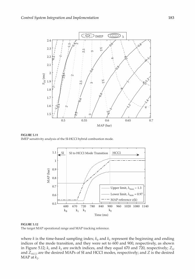
183Control System Integration and Implementation
where k is the time-based sampling index; kB and kE represent the beginning and ending indices of the mode transition, and they were set to 600 and 900, respectively, as shown in Figure 5.12; k1 and k2 are switch indices, and they equal 670 and 720, respectively; ZSI and ZHCCI are the desired MAPs of SI and HCCI modes, respectively; and Z is the desired MAP at k2.
0.5 1
11.5
1.5
1.5
2
22
2.5
2.5
2.5
33
33.5
3.53.5
4
4
4
4.5
4.5
5
MAP (bar)
F DI (
ms)
0.4
0.4
0.40.6
0.6
0.6
0.8
0.8
0.8
1
1
1
1.2
1.21.4
0.5 0.55 0.6 0.65 0.7
1.5
1.6
1.7
1.8
1.9
2
2.1
2.2
2.3
2.4IMEP λ
FIGURE 5.11IMEP sensitivity analysis of the SI-HCCI hybrid combustion mode.
600 670 720 780 840 900 960 1020 1080 11400.5
0.6
0.7
0.8
0.9
1
1.1
Time (ms)
MA
P (b
ar)
Upper limit, λmax = 1.3
Lower limit, λmin = 0.97MAP reference z(k)
SI HCCI
k2k1kB kE
SI to HCCI Mode Transition
FIGURE 5.12The target MAP operational range and MAP tracking reference.
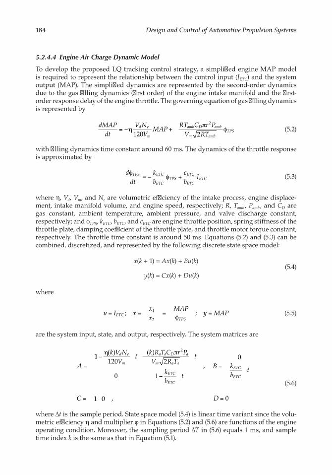
184 Design and Control of Automotive Propulsion Systems
5.2.4.4 Engine Air Charge Dynamic Model
To develop the proposed LQ tracking control strategy, a simplified engine MAP model is required to represent the relationship between the control input (IETC) and the system output (MAP). The simplified dynamics are represented by the second-order dynamics due to the gas filling dynamics (first order) of the engine intake manifold and the first-order response delay of the engine throttle. The governing equation of gas filling dynamics is represented by
dMAP
dtV N
VMAP
RT C r PV RT
d e
m
amb D amb
m ambTPS120 2
2
= −η +π
φ (5.2)
with filling dynamics time constant around 60 ms. The dynamics of the throttle response is approximated by
ddt
kb
cb
ITPS ETC
ETCTPS
ETC
ETCETC
φ= − φ + (5.3)
where η, Vd, Vm, and Ne are volumetric efficiency of the intake process, engine displace-ment, intake manifold volume, and engine speed, respectively; R, Tamb , Pamb , and CD are gas constant, ambient temperature, ambient pressure, and valve discharge constant, respectively; and ϕTPS, kETC, bETC, and cETC are engine throttle position, spring stiffness of the throttle plate, damping coefficient of the throttle plate, and throttle motor torque constant, respectively. The throttle time constant is around 50 ms. Equations (5.2) and (5.3) can be combined, discretized, and represented by the following discrete state space model:
x(k + 1) = Ax(k) + Bu(k)
y(k) = Cx(k) + Du(k) (5.4)
where
u I xxx
MAPy MAPETC
TPS= = =
φ=; ;1
2 (5.5)
are the system input, state, and output, respectively. The system matrices are
1( )120
( )2
0 1,
0
1 0 , 0
2
A
k V NV
tk R T C r PV R T
t
kb
t
B kb
t
C D
d e
m
a a D a
m a a
ETC
ETC
ETC
ETC
=
−η π
−
=
= =
(5.6)
where Δt is the sample period. State space model (5.4) is linear time variant since the volu-metric efficiency η and multiplier φ in Equations (5.2) and (5.6) are functions of the engine operating condition. Moreover, the sampling period ΔT in (5.6) equals 1 ms, and sample time index k is the same as that in Equation (5.1).

185Control System Integration and Implementation
5.2.4.5 LQ Tracking Control Design
Based on the control-oriented engine MAP model, a finite horizon LQ optimal tracking controller was designed to follow the reference z(k). More specifically, the control objective is to minimize the tracking error e(k) defined in (5.7) with the feasible control effort IETC. The tracking error e(k) is defined as
e(k) = y(k) − z(k) = Cx(k) − z(k) (5.7)
and the constraint on IETC is –5A < IETC < 5A. The cost function of the LQ optimal controller is defined as
∑ { }
= − −
+ − − +=
= −
12
[ ( ) ( )] [ ( ) ( )]
12
[ ( ) ( )] [ ( ) ( )] ( ) ( )1
J Cx k z k F Cx k z k
Cx k z k Q Cx k z k u k Ru k
f fT
f f
T T
k k
k k
i
f (5.8)
where F and Q are positive semidefinite and R is positive definite. For this design, F and Q are constant matrices defined in (5.9), and R is a function of sample index and tuned to minimize the tracking error with feasible throttle control effort (see Figure 5.13).
F = 10−8, Q = 4 × 10⁻⁷, R = R(k) (5.9)
Based on the cost function, the corresponding Hamiltonian is as follows:
H Cx k z k Q Cx k z k u k Ru k
p k Ax k Bu k
T T
T
12
[ ( ) ( )] [ ( ) ( )]12
( ) ( )
( 1) ( ) ( )[ ]
= − − +
+ + +
(5.10)
According to [28], the necessary conditions for the extremum in terms of the Hamiltonian are represented as
H
p kx k x k Ax k Bu k
( 1)( 1) ( 1) ( ) ( )*
* * * *∂∂ +
= + + = + (5.11)
600 660 720 780 840 9000
0.5
1
1.5
Sampling Index k, Time (ms)
R
FIGURE 5.13Adjustment of weighting matrix R.

186 Design and Control of Automotive Propulsion Systems
H
x kp k p k A p k C QCx k C Qz kT T T
( )( ) ( ) ( 1) ( ) ( )*
* * * *∂∂
= = + + − (5.12)
H
u kB p k Ru kT
( )0 0 ( 1) ( )*
* *∂∂
= = + + (5.13)
Note that the * denotes the optimal trajectories of the corresponding vectors. The aug-mented system of (5.11) and (5.12) becomes
x k
p k
A BR BC QC A
x k
p k C Qz k
T
T T T
( 1)
( )
( )
( 1)
0( )
*
*
1 *
*
+=
−
++
−
−
(5.14)
Based on Equation (5.13), the optimal control is in the form of
u*(k) = −R−1BT[P(k)x*(k) − g(k)] (5.15)
Matrix P(k) can be computed by solving the difference Riccati equation backwards,
P(k) = ATP(K + 1)[I + EP(K + 1)]−1 A + CTQC (5.16)
with the terminal condition
P(kf) = CTFC (5.17)
and vector g(k) can be computed by solving the vector difference equation
g(k) = AT{I − [P −1(k + 1) + E]−1E} g(k + 1) + CTQz(k) (5.18)
with the terminal condition
g(kf) = CTFz(kf) (5.19)
The optimal control in Equation (5.15) can be written into the following form:
u*(k) = −LFB(k)x*(k) + LFF(k)g(k + 1) (5.20)
where the feedforward gain LFF is computed by
LFF(k) = [R + BTP(k + 1)B]−1BT (5.21)
and the feedback gain LFB is computed by
LFB(k) = [R + BTP(k + 1)B]−1BTP(k + 1)A (5.22)
Note that in Equation (5.20) the state x* used in the feedback control is computed exactly from the closed-loop system model defined below:
x*(k + 1) = [A − BLFB(k)]x*(k) + BLFF(k)g(k + 1) (5.23)
However, when the control is implemented into the CIL simulation environment or the actual engine control system, the feedback states are replaced by the actual signals
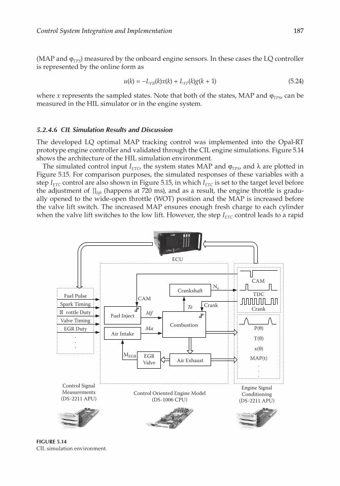
187Control System Integration and Implementation
(MAP and φTPS) measured by the onboard engine sensors. In these cases the LQ controller is represented by the online form as
u(k) = −LFB(k)x(k) + LFF(k)g(k + 1) (5.24)
where x represents the sampled states. Note that both of the states, MAP and φTPS, can be measured in the HIL simulator or in the engine system.
5.2.4.6 CIL Simulation Results and Discussion
The developed LQ optimal MAP tracking control was implemented into the Opal-RT prototype engine controller and validated through the CIL engine simulations. Figure 5.14 shows the architecture of the HIL simulation environment.
The simulated control input IETC, the system states MAP and φTPS, and λ are plotted in Figure 5.15. For comparison purposes, the simulated responses of these variables with a step IETC control are also shown in Figure 5.15, in which IETC is set to the target level before the adjustment of Πlift (happens at 720 ms), and as a result, the engine throttle is gradu-ally opened to the wide-open throttle (WOT) position and the MAP is increased before the valve lift switch. The increased MAP ensures enough fresh charge to each cylinder when the valve lift switches to the low lift. However, the step IETC control leads to a rapid
Combustion
TeFuel Inject
Air Intake
Mf
Ma
EGRValve
Ne
MEGR
Control Oriented Engine Model(DS-1006 CPU)
Engine SignalConditioning
(DS-2211 APU)
Control SignalMeasurements(DS-2211 APU)
Fuel PulseSpark Timing�rottle DutyValve Timing
EGR Duty
ECU
Crankshaft TDC
CAM
Crank
P(θ)
T(θ)
x(θ)
.
.
.
Air Exhaust
.
.
.
MAP(t)
CAMCrank
FIGURE 5.14CIL simulation environment.

188 Design and Control of Automotive Propulsion Systems
increment of the engine MAP or excessive fresh air charge, leading to an extremely lean air-to-fuel ratio λ in the following engine cycles.
Using the proposed LQ MAP tracking control strategy, throttle current IETC is regulated in a nonmonotonic increasing pattern. Note that to maintain IETC in the feasible range (–5A < IETC < 5A), the weighting matrix R in the cost function (5.8) is adjusted as illustrated in Figure 5.13. The similar pattern can also be found for φTPS with a small phase lag. As a result, the engine MAP tracks the reference z(k) after the intake valve lift Πlift switches to the low lift, and λ of each cylinder is successfully maintained within the desired range. Therefore, with the help of the LQ optimal tracking control, the in-cylinder air-to-fuel ratio is maintained within the desired range, leading to stable combustion.
Slight oscillations in the MAP responses are found with both control approaches, which are due to the flow dynamics of the engine air handling system and the engine MAP modeling error. It is almost impossible to eliminate them. Moreover, the MAP oscillation associated with the LQ optimal tracking control is within the desired MAP range.
5.3 Control System Calibration and Integration
Control system integration involves the process of controller calibration to tune the con-trol to provide robust stability and desired performance and to meet the fuel economy through dynamometer and vehicle tests. The dynamometer test is often considered an
–20246
I ETC
(A)
0
50
100
0.6
0.8
1
MA
P (b
ar)
w/o LQw/LQ
z(k)
600 750 900 1050 1200 1350 1500 16501
1.2
1.4
Time (ms)
Cylinder #1Cylinder #2Cylinder #3Cylinder #4
φ TPS
(%)
λ
λminλmax
FIGURE 5.15Engine performances of the optimal MAP tracking control.
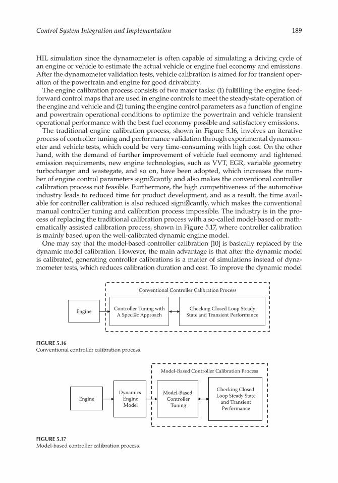
189Control System Integration and Implementation
HIL simulation since the dynamometer is often capable of simulating a driving cycle of an engine or vehicle to estimate the actual vehicle or engine fuel economy and emissions. After the dynamometer validation tests, vehicle calibration is aimed for for transient oper-ation of the powertrain and engine for good drivability.
The engine calibration process consists of two major tasks: (1) fulfilling the engine feed-forward control maps that are used in engine controls to meet the steady-state operation of the engine and vehicle and (2) tuning the engine control parameters as a function of engine and powertrain operational conditions to optimize the powertrain and vehicle transient operational performance with the best fuel economy possible and satisfactory emissions.
The traditional engine calibration process, shown in Figure 5.16, involves an iterative process of controller tuning and performance validation through experimental dynamom-eter and vehicle tests, which could be very time-consuming with high cost. On the other hand, with the demand of further improvement of vehicle fuel economy and tightened emission requirements, new engine technologies, such as VVT, EGR, variable geometry turbocharger and wastegate, and so on, have been adopted, which increases the num-ber of engine control parameters significantly and also makes the conventional controller calibration process not feasible. Furthermore, the high competitiveness of the automotive industry leads to reduced time for product development, and as a result, the time avail-able for controller calibration is also reduced significantly, which makes the conventional manual controller tuning and calibration process impossible. The industry is in the pro-cess of replacing the traditional calibration process with a so-called model-based or math-ematically assisted calibration process, shown in Figure 5.17, where controller calibration is mainly based upon the well-calibrated dynamic engine model.
One may say that the model-based controller calibration [10] is basically replaced by the dynamic model calibration. However, the main advantage is that after the dynamic model is calibrated, generating controller calibrations is a matter of simulations instead of dyna-mometer tests, which reduces calibration duration and cost. To improve the dynamic model
Engine
Conventional Controller Calibration Process
Controller Tuning withA Speci�c Approach
Checking Closed Loop SteadyState and Transient Performance
FIGURE 5.16Conventional controller calibration process.
Engine
Model-Based Controller Calibration Process
Model-Based Controller
Tuning
Checking Closed Loop Steady State
and Transient Performance
Dynamics Engine Model
FIGURE 5.17Model-based controller calibration process.

190 Design and Control of Automotive Propulsion Systems
calibration duration, the design of experiments (DOE) [11] is often used to reduce the associated dynamic model calibration duration [29], that is, to reduce the number of dynamometer tests required to calibrate the dynamic engine using the DOE optimization technique.
References
1. S. Pace and G. Zhu, Transient Air-to-Fuel Ratio Control of an SI Engine Using Linear Quadratic Tracking, Journal of Dynamic System, Measurement, and Control, 136(2): 021008, 2014. DOI: 10.1115/1.4025858.
2. S. Pace and G. Zhu, Sliding Mode Control of Both Air-to-Fuel and Fuel Ratios for a Dual-Fuel Internal Combustion Engine, Journal of Dynamic Systems, Measurement, and Control, 134(3): 031012, 2012, DOI: 10.1115/1.4005513.
3. A. White, G. Zhu, and J. Choi, Hardware-in-the-Loop Simulation of Robust Gain-Scheduling Control of Port-Fuel-Injection Process, IEEE Transactions on Control System Technology, 19(2), 1433–1443, 2011. DOI: 10.1109/TCST.2010.2095420.
4. G. Zhu, I. Haskara, and J. Winkelman, Closed Loop Ignition Timing Control Using Ionization Current Feedback, IEEE Transactions on Control System Technology, 15(3), 2007.
5. G. Zhu, I. Haskara, and J. Winkelman, Stochastic Limit Control and Its Application to Spark Limit Control Using Ionization Feedback, presented at Proceedings of the American Control Conference, Portland, OR, June 2005.
6. C.F. Daniels, G. Zhu, and J. Winkelman, Inaudible Knock and Partial-Burn Detection Using In-Cylinder Ionization Signal, SAE Technical Paper 2003-01-3149, 2003.
7. Z. Ren and G. Zhu, Modeling and Control of an Electrical Variable Valve Timing Actuator, Journal of Dynamic Systems, Measurement, and Control, 136(2), 021008, 2014. DOI: 10.1115/1.4025914.
8. A. White, Z. Ren, G. Zhu, and J. Choi, Mixed H∞ and H2 LPV Control of an IC Engine Hydraulic Cam Phase System, IEEE Transactions on Control System Technology, 21(1), 229–238, 2013. DOI: 10.1109/TCST.2011.2177464.
9. I. Haskara, G. Zhu, and J. Winkelman, Multivariable EGR/Spark Timing Control for IC Engines via Extremum Seeking, presented at Proceedings of the American Control Conference, Minneapolis, MN, June 2006.
10. M. Guerrier and P. Cawsey, The Development of Model Based Methodologies for Gasoline IC Engine Calibration, SAE Technical Paper 2004-01-1466, 2014.
11. S. Jiang, D. Nutter, and A. Gullitti, Implementation of Model-Based Calibration for a Gasoline Engine, SAE Technical Paper 2012-01-0722, 2012.
12. F. Zhao, T. Asmus, D. Assanis, J.E. Dec, J.A. Eng, and P.M. Najt, Homogeneous Charge Compression Ignition (HCCI) Engines Key Research and Development Issues, Warrendale, PA: Society of Automotive Engineers, 2003.
13. R.M. Wagner, K.D. Edwards, et al., Hybrid SI-HCCI Combustion Modes for Low Emissions in Stationary Power Applications, presented at 3rd Annual Advanced Stationary Reciprocating Engines Meeting, Argonne, IL, June 28–30, 2006.
14. N.J. Killingsworth, S.M. Aceves, et al., HCCI Engine Combustion-Timing Control: Optimizing Gains and Fuel Consumption via Extremum Seeking, IEEE Transactions on Control Systems Technology, 17(6), 1350–1361, 2009.
15. C.J. Chiang and A.G. Stefanopoulou, Stability Analysis in Homogeneous Charge Compression Ignition (HCCI) Engines with High Dilution, IEEE Transactions on Control System Technology, 15(2), 2007.
16. X. Yang and G. Zhu, A Two-Zone Control Oriented SI-HCCI Hybrid Combustion Model for the HIL Engine Simulation, presented at Proceedings of American Control Conference, San Francisco, CA, 2011.
191Control System Integration and Implementation
17. S.C. Kong and R.D. Reitz, Application of Detailed Chemistry and CFD for Predicting Direct Injection HCCI Engine Combustion and Emission, Proceedings of the Combustion Institute, 29: 663–669, 2002.
18. X. Yang, G. Zhu, and Z. Sun, A Control Oriented SI and HCCI Hybrid Combustion Model for Internal Combustion Engines, presented at Proceedings of ASME Dynamic Systems and Control Conference, Cambridge, MA, 2010.
19. N. Kalian, H. Zhao, and J. Qiao, Investigation of Transition between Spark Ignition and Controlled Auto-Ignition Combustion in a V6 Direct-Injection Engine with Cam Profile Switching, Journal of Automobile Engineering, 202, 2008.
20. N. Ravi, M.J. Roelle, et al., Model-Based Control of HCCI Engines Using Exhaust Recompression, IEEE Transactions on Control Systems Technology, 18(6), 1289–1302, 2010.
21. J. Kang, C. Chang, and T. Kuo, Sufficient Condition on Valve Timing for Robust Load Transients in HCCI Engines, SAE Technical Paper 2010-01-1243, 2010.
22. G.M. Shaver, Physics Based Modeling and Control of Residual-Affected HCCI Engines Using Variable Valve Actuation, PhD thesis, Stanford University, September 2005.
23. M.J. Roelle, G.M. Shaver, and J.C. Gerdes, Tackling the Transition: A Multi-Mode Combustion Model of SI and HCCI for Mode Transition Control, presented at Proceedings of IMECE International Mechanical Engineering Conference and Exposition, Anaheim, CA, November 13–19, 2004.
24. Y. Zhang, H. Xie, et al., Study of SI-HCCI-SI Transition on a Port Fuel Injection Engine Equipped with 4VVAS, SAE Technical Paper, SAE 2007-01-0199, 2007.
25. H. Wu, M. Kraft, et al., Experimental Investigation of a Control Method for SI-HCCI-SI Transition in a Multi-Cylinder Gasoline Engine, SAE Technical Paper, SAE 2010-01-1245, 2010.
26. X. Yang and G. Zhu, A Mixed Mean-Value and Crank-Based Model of a Dual-Stage Turbocharged SI Engine for Hardware-in-the-Loop Simulation, presented at Proceedings of the American Control Conference, Baltimore, MD, 2010.
27. X. Yang and G. Zhu, SI and HCCI Combustion Mode Transition Control of a Multi-Cylinder HCCI Capable SI Engine via Iterative Learning, presented at Proceedings of the 4th Annual Dynamic Systems and Control Conference, Arlington, VA, October 31–November 2, 2011.
28. D. Naidu, Optimal Control Systems, Boca Raton, FL: CRC Press, 2003, pp. 232–239. 29. M.-S. Vogels, J. Birnstingl, and T. Combe, Controller Calibration Using a Global Dynamic
Engine Model, presented at VortragVogels Workshop, Vienna, Austria, 2011.

6000 Broken Sound Parkway, NW Suite 300, Boca Raton, FL 33487711 Third Avenue New York, NY 100172 Park Square, Milton Park Abingdon, Oxon OX14 4RN, UK
an informa business
www.taylorandfrancisgroup.com
K11064
Better Understand the relationship Between powertrain system design and its Control integration
While powertrain system design and its control integration are traditionally divided into two different functional groups, a growing trend introduces the integration of more electronics (sensors, actuators, and controls) into the powertrain system. This has impacted the dynamics of the system, changing the traditional mechanical powertrain into a mechatronic powertrain, and creating new opportunities for improved efficiency. Design and Control of Automotive Propulsion Systems focuses on the ICE-based automotive powertrain system (while presenting the alternative powertrain systems where appropriate). Factoring in the multidisciplinary nature of the automotive propulsion system, this text does two things—adopts a holistic approach to the subject, especially focusing on the relationship between propulsion system design and its dynamics and electronic control, and covers all major propulsion system components, from internal combustion engines to transmissions and hybrid powertrains.
The book introduces the design, modeling, and control of the current automotive propulsion system, and addresses all three major subsystems: system level optimization over engines, transmissions, and hybrids (necessary for improving propulsion system efficiency and performance). It provides examples for developing control-oriented models for the engine, transmission, and hybrid. It presents the design principles for the powertrain and its key subsystems. It also includes tools for developing control systems and examples on integrating sensors, actuators, and electronic control to improve powertrain efficiency and performance. In addition, it presents analytical and experimental methods, explores recent achievements, and discusses future trends.
Comprised of five Chapters Containing the fUndamentals as well as new researCh, this text:
• Examines the design, modeling, and control of the internal combustion engine and its key subsystems:the valve actuation system, the fuel system, and the ignition system
• Expounds on the operating principles of the transmission system, the design of the clutch actuation system, and transmission dynamics and control
• Explores the hybrid powertrain, including the hybrid architecture analysis, the hybrid powertrain model, and the energy management strategies
• Explains the electronic control unit and its functionalities—the software-in-the-loop and hardware-in-the-loop techniques for developing and validating control systems
Design and Control of Automotive Propulsion Systems provides the background of the automotive propulsionsystem, highlights its challenges and opportunities, and shows the detailed procedures for calculating vehicle power demand and the associated powertrain operating conditions.
Automotive Engineering
D e s i g n a n d C o n t r o l o f AuTomoTIvE ProPulsIon sysTEms
Design and Control of AuTom
oTIvE Pro
PulsIon sysTEm
s
sunZhu
CAT#K11064 cover.indd 1 11/17/14 12:24 AM
