4.3 LINEAR REGRESSION WITH ONE INDEPENDENT VARIABLE

4.3.1 Basic Regression Model

First, examine a basic regression I:!J.illkl (or equ<ltion, which in this C<lse indicates the same thing):

Yi = bO + b I Xi + E i Eq ...t.3

where Yi = value of the dependent variable for the ith data point.

xi = value of the independent variable for the ith data point.

bO,b\ = constants (regression parameters),

E i =random error term, and

i = 1.2, 3..... n.

The above model is a simple, linear model. It is simple since there is only one independent variable (x). It is linear since both the parameters (bl), bl) <lnd the independent variable (x) are not power functions. (A non-linear model is one where the regression parameters ("constants") appear as exponents or when multiplied or divided by other parameters. Further, other types of non-linear models are ones where the independent variable(s) are second order powers (or higher). Non-linear models will be illustrated in Sections 4.3.7, 4.3.8, and 4.3.9.)

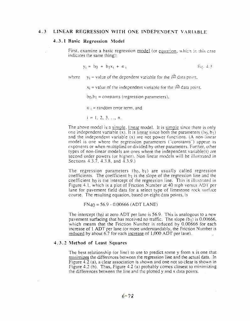
The regression parameters (bo, bl) are usually called regression coefficients. The coefficient b I is the slope of the regression line and the coefficient bO is the intercept of the regression line. This is illustrated in Figure 4.1, which is a plot of Friction Number at 40 mph versus ADT per lane for pavement field data for a select type of limestone rock surface course. The resulting equation, based on eight data points, is

FN40 =56.9 - 0.00666 (ADT LANE)

The intercept (bO) at zero ADT per lane is 56.9. This is analogous to a new pavement surfacing that has received no traffic. The slope (b I) is 0.00666, which means that the Friction Number is reduced by 0.00666 for each increase of 1 ADT per lane (or more understandably, the Friction Number is reduced by about 6.7 for each increase of 1,000 ADT per lane).

4.3.2 Method of Least Squares

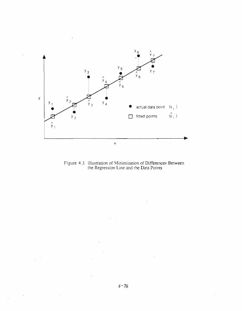
The best relationship (or line) to use to predicl.Some y from x is one that minimizes the differences between the regression line and the actual data. In Figure 4.2 (a), a clear association is shown and one not so clear is shown in Figure 4.2 (b). Thus, Figure 4.2 (a) probably comes closest to minimizing the differences between the line and the plotted y and x data points.

6-7~

60 b = 569O

~

FN 40 = 569 - 000666 (ADTilane)

250 R = 077

(original data points not available)

40

<3 «r

z b[ = 000666 /l.J...

~

.3 30 E :::J C C 0

D 'C l.J...

20

10

~0L.- __L. ___l .L._ ___..J

o 1000 2000 3000 4000 5000

AOT/lane

Figure 4.1. Friction Numbers versus ADT per Lane for Select Limestone Rock Surfaces

•. .

Y6 1\

Y 1\ •Y1 • actual data point (y i )

1\

fitted points (y i )Y2• 0

1\

Y1

• Y4Y3

x

Figure 4.3. Illustration of Minimization of Differences Between the Regression Line and the Data Points

6-76

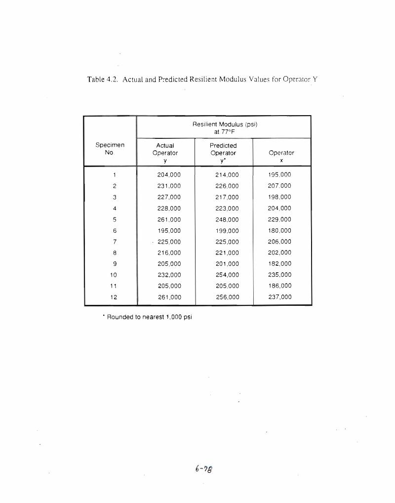
Table 4.2. Actual and Predicted Resilient Modulus Values for Operator Y

Specimen No.

Resilient Modulus (psi) at 77°F

Actual Operator

y

Predicted Operator

y' Operator

x

1 204,000 214,000 195,000

2 231,000 226,000 207,000

3 227,000 217,000 198,000

4 228,000 223,000 204,000

5 261,000 248,000 229,000

6 195,000 199,000 180,000

7 225,000 225,000 206,000

8 216.000 221.000 202.000

9 205,000 201,000 182,000

10 232.000 254.000 235.000

11 205,000 205,000 186,000

12 261,000 256.000 237.000

• Rounded to nearest 1,000 psi

6-?B

Stated another way, the SSE is the amount of the sum of squares

best explained by the mean (f) of the dependent variable. The SSE

=SSTO when all y =y. 4.3.4.3 Regression sum of squares (SSR)

Hopefully, for a regression line you wish to develop, the SSTO is much larger than the SSE. The difference is termed the regression sum of squares (SSR):

n SSR = I (Yi - y)2

i=l

These deviations are illustrated by the dashed lines shown in Figure 4.4 (c). Since the SSR is composed of deviations between the "fitted" regression line and the mean of the data points, the larger the SSR the better the ftt of the regression line to the data. Stated another way, the SSR is the amount of the sum of squares explained by the regression equation. For Figure 4.4 (c), SSR is

SSR = (Yl - y)2 + (Y2 - y)2 + (93 - y)2 + (Y4 - y)2 + (Y5 - )7)2

4.3.4.4 Final overview of sum of squares

From the previous sections, we can see that

1\ -Yi - Y + Yi - Yi

total deviation devia tion of fined deviation around regression value the regression line about the mean

or L (Yi - )7)2 = L (Yi - y)2 + L (Yi - Yi)2

SSTO = SSR + SSE

4.3.5 Regression line "goodness.of.fit"

4.3.5.1 Coefficient of determination (R2)

The R2 value explains how much of the total variation in the data is explained by the regression line. Stated another way, the R2 measures the reduction in the total variation for "y" associated with the use of "x". The R2 = 1.0 when all data points fall on the regression line, as shown in Figure 4.5(a). The R2 = a when the regression line matches the average (or mean) of the data points, as illustrated in Figure 4.5 (b). [n other words the mean of the data points is as good a predictor of "y" as any line fit through the data points.

6-80

For example, if R2 = 0.20. then the total variation in y is reduced by

only 20 percent when x is used (on the other hand r = '1/ R '2 = 'I () 2 = 0.45).

4.3.5.2 Mean square error (MSE) and root mean square error (RMSE)

The mean square error is calculated as follows:

MSE _ SSE _ SSE - error degrees of freedom - n-2

The root mean square error is simply the square root of MSE:

RMSE = ~MSE

The RMSE is the standard deviation of the distribution of y for a specific x. Stated another way, the RMSE is the standard deviation of the regression line. The larger the RMSE for a specific regression equation, the poorer the associated predictions.

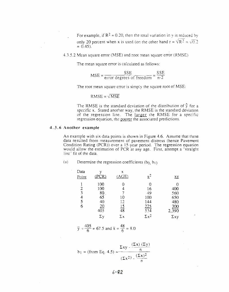
4.3.6 Another example

An example with six data points is shown in Figure 4.6. Assume that these data resulted from measurement of pavement distress (hence Pavement Condition Rating (PCR)) over a IS-year period. The regression equation would allow the estimation of PCR at any age. First, attempt a "straight line" fit of the data.

(a) Determine the regression coefficients (bo, bl)

Data y x Point ill:Rl CAGE) ~2

1 100 0 0 o 2 100 4 16 400 3 80 _ 7 49 S60 4 65 10 100 650 5 40 12 144 480 6 20 12 225 .1QQ

405 48 534 2,390

~y LX ~x2 ~xy

Y= 4~5 = 67.5 and x=~ = R.O

~ (~x) (~y) xy - n

b I = (from Eq. 4.5) =------­(~x2) _ (~x)2

n

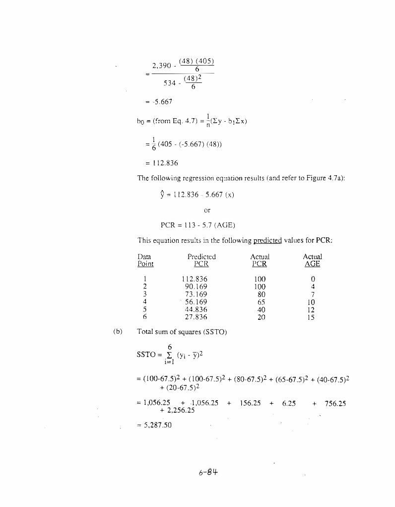
2,390 _ (48) ~405)

= 534 (48)2

- 6

= -5.667

1bo = (from Eq. 4.7) =-(Iy - blIx)

n

= ~ (405 - (-5.667) (48))

= 112.836

The following regression equation results (and refer to Figure 4.7a):

y= 112.836 - 5.667 (x)

or

PCR = 113 - 5.7 (AGE)

This equation results in the following predicted values for PCR:

Data Predicted Actual Actual Point PCR PCR AGE

1 112.836 100 0 2 90.169 100 4 3 73.169 80 7 4 56.169 65 10 5 44.836 40 12 6 27.836 20 15

(b) Total sum of squares (SSTO)

6 SSTO = I (Yi - y)2

i=l

= (100-67.5)2 + (100-67.5)2 + (80-67.5)2 + (65-67.5)2 + (40-67.5)2 + (20-67.5)2

= 1,056.25 + .1,056.25 + 156.25 + 6.25 + 756.25 + 2,256.25

= 5.287.50

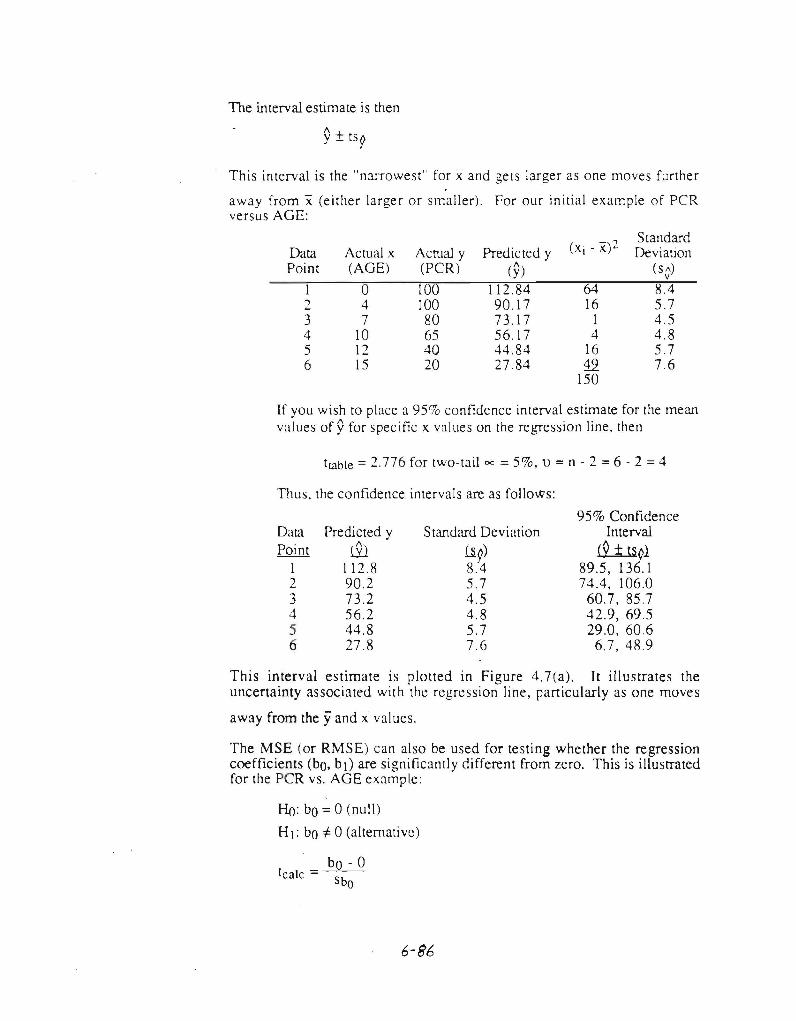
The interval estimate is then

This interval is the "narrowest" for xand gets larger as one moves further

away from x: (either larger or smaller). For our initial example of PCR versus AGE:

Data Actual x Actual y Predicted y (Xi - x)2 Standard Deviation

Point (AGE) (PCR) (y) (s A) V

1 0 100 112.84 64 8.4 2 4 100 90.17 16 5.7 3 7 80 73.17 1 4.5 4 10 65 56.17 4 4.8 5 12 40 44.84 16 5.7 6 15 20 27.84 12 7.6

150

If you wish to place a 95% confidence interval estimate for the mean values of yfor specific x vCllues on the regression line, then

twble = 2.776 for two-tail oc = 5%, 1) = n - 2 =6 - 2 = 4

Thus, the confidence intervals are as follows:

95% Confidence Data Predicted y Standard Deviation Interval Point W U9) fll..uql

1 112.8 8.4 89.5,136.1 2 90.2 5.7 74.4, 106.0 3 73.2 4.5 60.7, 85.7 4 56.2 4.8 42.9, 69.5 5 44.8 5.7 29.0, 60.6 6 27.8 7.6 6.7,48.9

This interval estimate is plotted in Figure 4.7(a). It illustrates the uncertainty associated with the regression line, particularly as one moves

away from the yand xvalues.

The MSE (or RMSE) can also be used for testing whether the regression coefficients (bO. bl) are significantly different from zero. This is illustrated for the peR vs. AGE example:

Ho: bO = 0 (null)

HI: bO f:. 0 (alternative)

bO - 0 tcalc =

Sbo

6-8b

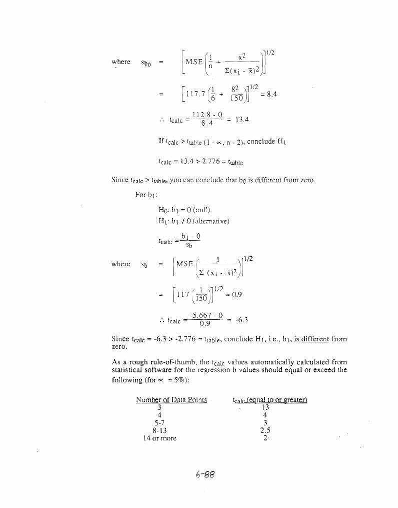
where = [MSE (l + _xLJ]I12 n L.(xi- x)2

82)] 1/2= [ 117.7 1

=8.4(6 + 150

If tealc > ttable (l - ex, n - 2), conclude HI

teak = 13.4> 2.776 = ttable

Since tealc > tlable, you can conclude that bo is different from zero.

HO: bl = 0 (null)

HI: bl f. 0 (alternative)

b I - 0tcalc sb

)rwhere sb = [MSE ( I L. (Xi - x)2

= [117 (I~O)r/2=0.9

-5.667 - 0 _ -63:. tealc 0.9 -.

Since teak = -6.3 > -2.776 = ttable, conclude HI, i.e., bl, is different from zero.

As a rough rule-of-thumb, the tcalc values automatically calculated from statistical software for the regression b values should equal or exceed the following (for ex =5%):

Number of Data Points tealc (equal to or greater) 3 13 4 4

5-7 3 8-13 2.5

14 or more 2·