linear discriminant analysis c jonathan...

Statistics 202:Data Mining

c©JonathanTaylor

Statistics 202: Data MiningLinear Discriminant Analysis

Based in part on slides from textbook, slides of Susan Holmes

c©Jonathan Taylor

November 9, 2012

1 / 1


c©JonathanTaylor

Discriminant analysis

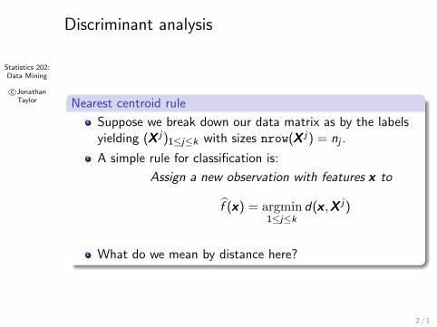
Nearest centroid rule

Suppose we break down our data matrix as by the labelsyielding (XXX j)1≤j≤k with sizes nrow(XXX j) = nj .

A simple rule for classification is:

Assign a new observation with features xxx to

f (xxx) = argmin1≤j≤k

d(xxx ,XXX j)

What do we mean by distance here?

2 / 1


c©JonathanTaylor



If we can assign a central point or centroid µj to each XXX j ,then we can define the distance above as distance to thecentroid µj .

This yields the nearest centroid rule

f (xxx) = argmin1≤j≤k

d(xxx , µj)

3 / 1


c©JonathanTaylor



This rule is described completely by the functions

hij(xxx) =d(xxx , µj)

d(xxx , µi )

with f (xxx) being any i such that

hij(xxx) ≥ 1 ∀j .

4 / 1


c©JonathanTaylor



If d(xxx ,yyy) = ‖x − y‖2 then the natural centroid is

µj =1

nj

nj∑l=1

XXX jl

This rule just classifies points to the nearest µj .

But, if the covariance matrix of our data is not I , this ruleignores structure in the data . . .

5 / 1


c©JonathanTaylor

Why we should use covariance

3 2 1 0 1 2 35

0

5

10

15

20

6 / 1


c©JonathanTaylor


Choice of distance

Often, there is some background model for our data thatis equivalent to a given procedure.

For this nearest centroid rule, using the Euclidean distanceeffectively assumes that within the set of points XXX j , therows are multivariate Gaussian with covariance matrixproportional to I .

It also implicitly assumes that the nj ’s are roughly equal.

For instance, if one nj was very small just because a datapoint is close to that µj doesn’t necessarily mean that weshould conclude it has label j because there might be ahuge number of points of label i near that µj .

7 / 1


c©JonathanTaylor


Gaussian discriminant functions

Suppose each group with label j had its own mean µj andcovariance matrix Σj , as well as proportion πj .

The Gaussian discriminant functions are defined as

hij(xxx) = hi (xxx)− hj(xxx)

hi (xxx) = log πi − log |Σi |/2− (xxx − µi )TΣ−1i (xxx − µi )/2

The first term weights the prior probability, the second twoterms are log φµi ,Σi

(xxx) = log L(µi ,Σi |xxx).

Ignoring the first two terms, the hi ’s are essentiallywithin-group Mahalanobis distances . . .

8 / 1


c©JonathanTaylor


Gaussian discriminant functions

The classifier assigns xxx label i if hi (xxx) ≥ hj(xxx)∀j .Or,

f (xxx) = argmax1≤i≤k

hi (xxx)

This is equivalent to a Bayesian rule. We’ll see moreBayesian rules when we talk about naıve Bayes . . .

When all Σi and πi ’s are identical, the classifier is justnearest centroid using Mahalanobis distance instead ofEuclidean distance.

9 / 1


c©JonathanTaylor


Estimating discriminant functions

In practice, we will have to estimate πj , µj ,Σj .

Obvious estimates:

πj =nj∑kj=1 nj

µj =1

nj

nj∑l=1

XXX jl

Σj =1

nj − 1(XXX j − µj111)T (XXX j − µj111)

10 / 1


c©JonathanTaylor


Estimating discriminant functions

If we assume that the covariance matrix is the same withingroups, then we might also form the pooled estimate

ΣP =

∑kj=1(nj − 1)Σj∑k

j=1 nj − 1

If we use the pooled estimate Σj = ΣP and plug these intothe Gaussian discrimants, the functions hij(xxx) are linear(or affine) functions of xxx .

This is called Linear Discriminant Analysis (LDA).

Not to be confused with the other LDA (Latent DirichletAllocation) . . .

11 / 1


c©JonathanTaylor

Linear Discriminant Analysis using (petal.width,petal.length)

0 1 2 3 4 5 6 7 80.5

0.0

0.5

1.0

1.5

2.0

2.5

3.0

12 / 1


c©JonathanTaylor

Linear Discriminant Analysis using (sepal.width,sepal.length)

3.5 4.0 4.5 5.0 5.5 6.0 6.5 7.0 7.5 8.02.0

2.5

3.0

3.5

4.0

4.5

5.0

13 / 1


c©JonathanTaylor


Quadratic Discriminant Analysis

If we use don’t use pooled estimate Σj = Σj and plugthese into the Gaussian discrimants, the functions hij(xxx)are quadratic functions of xxx .

This is called Quadratic Discriminant Analysis (QDA).

14 / 1


c©JonathanTaylor

Quadratic Discriminant Analysis using(petal.width, petal.length)

0 1 2 3 4 5 6 7 80.5

0.0

0.5

1.0

1.5

2.0

2.5

3.0

15 / 1


c©JonathanTaylor

Quadratic Discriminant Analysis using(sepal.width, sepal.length)

3.5 4.0 4.5 5.0 5.5 6.0 6.5 7.0 7.5 8.02.0

2.5

3.0

3.5

4.0

4.5

5.0

16 / 1


c©JonathanTaylor

Motivation for Fisher’s rule

3 2 1 0 1 2 35

0

5

10

15

20

17 / 1


c©JonathanTaylor


Fisher’s discriminant function

Fisher proposed to classify using a linear rule.

He first decomposed

(XXX − µ111)T (XXX − µ111) = SSB + SSW

Then, he proposed,

v = argmaxv :vT SSW v=1

vT SSBv

Having found v , form XXX j v and the centroidηj = mean(XXX j v)

In the two-class problem k = 2, this is the same as LDA.

18 / 1


c©JonathanTaylor


Fisher’s discriminant functions

The direction v1 is an eigenvector of some matrix. Thereare others, up to k − 2 more.

Suppose we find all k − 1 vectors and form XXX jVT , each

one an nj × (k − 1) matrix with centroid ηj ∈ Rk−1.

The matrix V determines a map from Rp to Rk−1, sogiven a new data point we can compute Vxxx ∈ Rk−1.

This gives rise to a classifier

f (xxx) = nearest centroid(Vxxx)

This is LDA (assuming πj = 1k ) . . .

19 / 1


c©JonathanTaylor


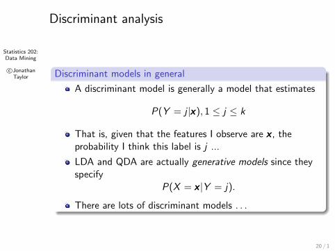
Discriminant models in general

A discriminant model is generally a model that estimates

P(Y = j |xxx), 1 ≤ j ≤ k

That is, given that the features I observe are xxx , theprobability I think this label is j ...

LDA and QDA are actually generative models since theyspecify

P(X = xxx |Y = j).

There are lots of discriminant models . . .

20 / 1


c©JonathanTaylor


Logistic regression

The logistic regression model is ubiquitous in binaryclassification (two-class) problems

Model:

P(Y = 1|xxx) =α + exxx

Tβ

1 + eα+xxxTβ= π(α, β,xxx)

21 / 1


c©JonathanTaylor


Logistic regression

Software that fits a logistic regression model produces anestimate of β based on a data matrix XXX n×p and binarylabels YYY n×1 ∈ {0, 1}n

It fits the model minimizing what we call the deviance

DEV(β) = −2n∑

i=1

(YYY i log π(β,XXX i )+(1−YYY i ) log(1−π(β,XXX i ))

While not immediately obvious, this is a convexminimization problem, hence is fairly easy to solve.

Unlike trees, the convexity yields a globally optimalsolution.

22 / 1


c©JonathanTaylor

Logistic regression, setosa vs virginica, versicolorusing (sepal.width, sepal.length)

3.5 4.0 4.5 5.0 5.5 6.0 6.5 7.0 7.5 8.02.0

2.5

3.0

3.5

4.0

4.5

5.0

23 / 1


c©JonathanTaylor

Logistic regression, virginica vs setosa, versicolorusing (sepal.width, sepal.length)

3.5 4.0 4.5 5.0 5.5 6.0 6.5 7.0 7.5 8.02.0

2.5

3.0

3.5

4.0

4.5

5.0

24 / 1


c©JonathanTaylor

Logistic regression, versicolor vs setosa, virginicausing (sepal.width, sepal.length)

3.5 4.0 4.5 5.0 5.5 6.0 6.5 7.0 7.5 8.02.0

2.5

3.0

3.5

4.0

4.5

5.0

25 / 1


c©JonathanTaylor


Logistic regression

Logistic regression produces an estimate of

P(yyy = 1|xxx) = π(xxx)

Typically, we classify as 1 if π(xxx) > 0.5.

This yields a 2× 2 confusion matrixPredicted: 0 Predicted: 1

Actual : 0 TN FP

Actual : 1 FN TP

From the 2× 2 confusion matrix, we can computeSensitivity, Specificity, etc.

26 / 1


c©JonathanTaylor


Logistic regression

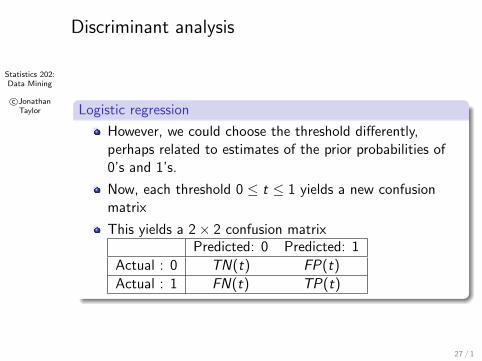
However, we could choose the threshold differently,perhaps related to estimates of the prior probabilities of0’s and 1’s.

Now, each threshold 0 ≤ t ≤ 1 yields a new confusionmatrix

This yields a 2× 2 confusion matrixPredicted: 0 Predicted: 1

Actual : 0 TN(t) FP(t)

Actual : 1 FN(t) TP(t)

27 / 1


c©JonathanTaylor


ROC curve

Generally speaking, we prefer classifiers that are bothhighly sensitive and highly specific.

These confusion matrices can be summarized using anROC (Receiver Operating Characteristic) curve.

This is a plot of the curve

(1− Specificity(t), Sensitivity(t))0≤t≤1

Often, Specificity is referred to as TNR (True NegativeRate), and (1− Specificity(t)) as FPR.

Often, Sensitivity is referred to as TPR (True PositiveRate), and (1− Sensitivity(t)) as FNR.

28 / 1


c©JonathanTaylor

AUC: Area under ROC curve

0.0 0.2 0.4 0.6 0.8 1.0False Positive Rate

0.0

0.2

0.4

0.6

0.8

1.0

Tru

e P

osi

tive R

ate

ROC curveRandom guessingt=0.5

29 / 1


c©JonathanTaylor


ROC curve

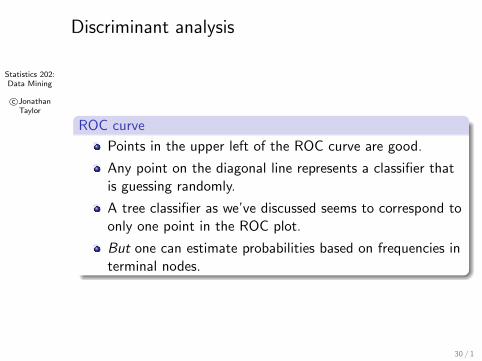
Points in the upper left of the ROC curve are good.

Any point on the diagonal line represents a classifier thatis guessing randomly.

A tree classifier as we’ve discussed seems to correspond toonly one point in the ROC plot.

But one can estimate probabilities based on frequencies interminal nodes.

30 / 1


c©JonathanTaylor


ROC curve

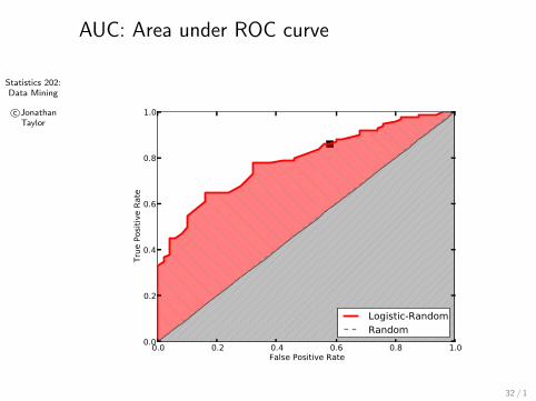
A common numeric summary of the ROC curve is

AUC (ROC curve) = Area under ROC curve.

Can be interpreted as an estimate of the probability thatthe classifier will give a random positive instance a higherscore than a random negative instance.Maximum value is 1.For a random guesser, AUC is 0.5

31 / 1


c©JonathanTaylor

AUC: Area under ROC curve

0.0 0.2 0.4 0.6 0.8 1.0False Positive Rate

0.0

0.2

0.4

0.6

0.8

1.0

Tru

e P

osi

tive R

ate

Logistic-RandomRandom

32 / 1

linear discriminant analysis c jonathan...

Documents