- p. 1/??

Statistics 203: Introduction to Regressionand Analysis of Variance

Course review

Jonathan Taylor

- p. 2/??

Today

■ Review / overview of what we learned.

- p. 3/??

General themes in regression models

■ Specifying regression models.◆ What is the joint (conditional) distribution of all outcomes

given all covariates?◆ Are outcomes independent (conditional on covariates)? If

not, what is an appropriate model?■ Fitting the models.

◆ Once a model is specified how are we going to estimatethe parameters?

◆ Is there an algorithm or some existing software to fit themodel?

■ Comparing regression models.◆ Inference for coefficients in the model: are some zero (i.e.

is a smaller model better?)◆ What if there are two competing models for the data? Why

would one be preferable to the other?◆ What if there are many models for the data? How do we

compare models for the data?

- p. 4/??

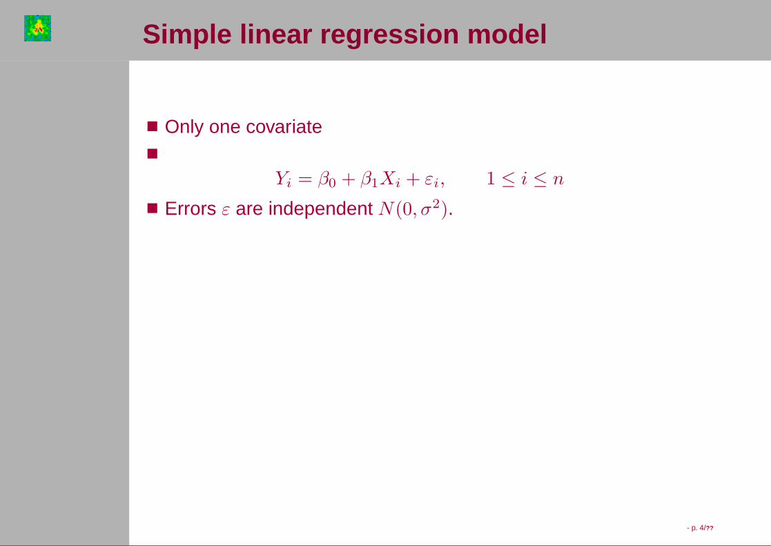
Simple linear regression model

■ Only one covariate■

Yi = β0 + β1Xi + εi, 1 ≤ i ≤ n

■ Errors ε are independent N(0, σ2).

- p. 5/??

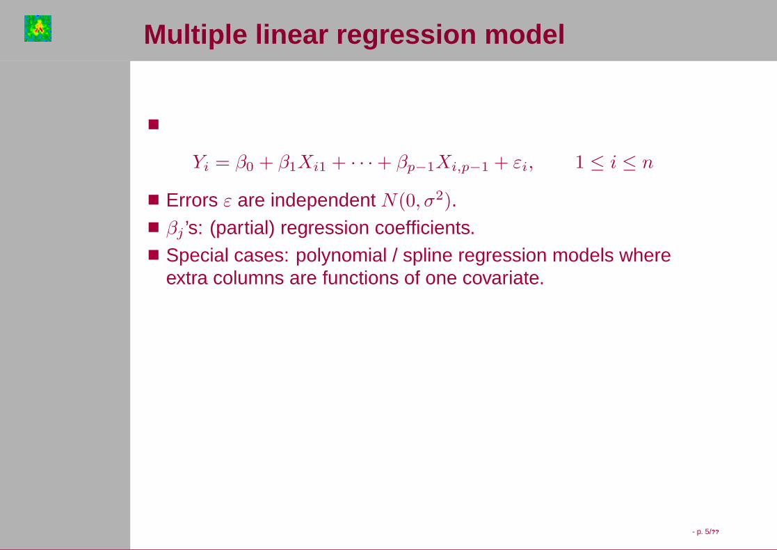
Multiple linear regression model

■

Yi = β0 + β1Xi1 + · · · + βp−1Xi,p−1 + εi, 1 ≤ i ≤ n

■ Errors ε are independent N(0, σ2).■ βj ’s: (partial) regression coefficients.■ Special cases: polynomial / spline regression models where

extra columns are functions of one covariate.

- p. 6/??

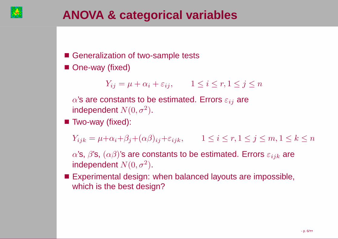
ANOVA & categorical variables

■ Generalization of two-sample tests■ One-way (fixed)

Yij = µ+ αi + εij , 1 ≤ i ≤ r, 1 ≤ j ≤ n

α’s are constants to be estimated. Errors εij areindependent N(0, σ2).

■ Two-way (fixed):

Yijk = µ+αi+βj+(αβ)ij+εijk, 1 ≤ i ≤ r, 1 ≤ j ≤ m, 1 ≤ k ≤ n

α’s, β’s, (αβ)’s are constants to be estimated. Errors εijk areindependent N(0, σ2).

■ Experimental design: when balanced layouts are impossible,which is the best design?

- p. 7/??

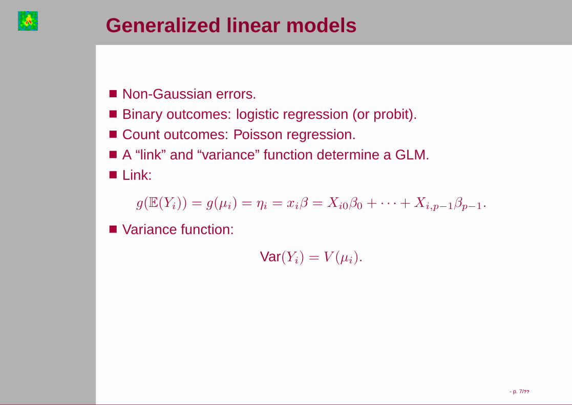
Generalized linear models

■ Non-Gaussian errors.■ Binary outcomes: logistic regression (or probit).■ Count outcomes: Poisson regression.■ A “link” and “variance” function determine a GLM.■ Link:

g(E(Yi)) = g(µi) = ηi = xiβ = Xi0β0 + · · · +Xi,p−1βp−1.

■ Variance function:

Var(Yi) = V (µi).

- p. 8/??

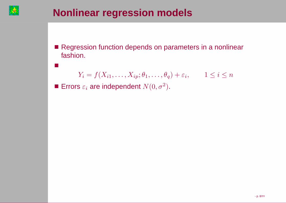
Nonlinear regression models

■ Regression function depends on parameters in a nonlinearfashion.

■

Yi = f(Xi1, . . . , Xip; θ1, . . . , θq) + εi, 1 ≤ i ≤ n

■ Errors εi are independent N(0, σ2).

- p. 9/??

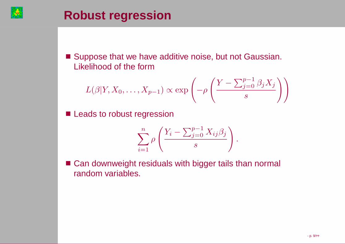
Robust regression

■ Suppose that we have additive noise, but not Gaussian.Likelihood of the form

L(β|Y,X0, . . . , Xp−1) ∝ exp

(−ρ

(Y −

∑p−1j=0 βjXj

s

))

■ Leads to robust regression

n∑

i=1

ρ

(Yi −

∑p−1j=0 Xijβj

s

).

■ Can downweight residuals with bigger tails than normalrandom variables.

- p. 10/??

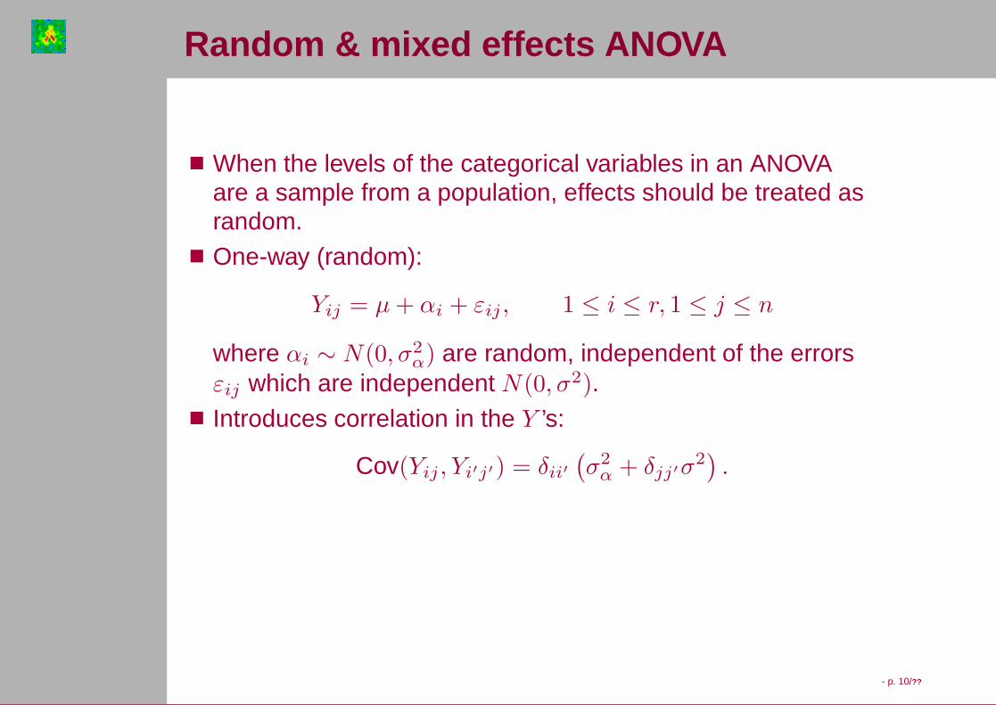
Random & mixed effects ANOVA

■ When the levels of the categorical variables in an ANOVAare a sample from a population, effects should be treated asrandom.

■ One-way (random):

Yij = µ+ αi + εij , 1 ≤ i ≤ r, 1 ≤ j ≤ n

where αi ∼ N(0, σ2α) are random, independent of the errors

εij which are independent N(0, σ2).■ Introduces correlation in the Y ’s:

Cov(Yij , Yi′j′) = δii′(σ2

α + δjj′σ2).

- p. 11/??

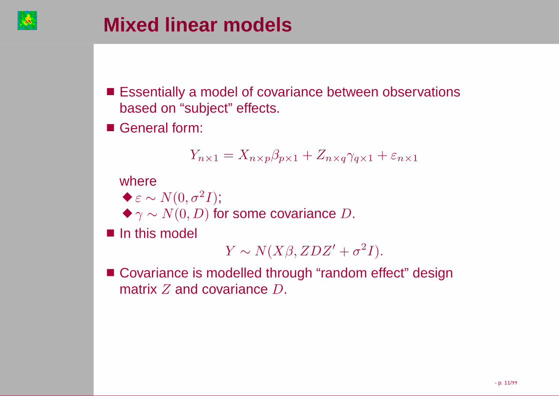
Mixed linear models

■ Essentially a model of covariance between observationsbased on “subject” effects.

■ General form:

Yn×1 = Xn×pβp×1 + Zn×qγq×1 + εn×1

where◆ ε ∼ N(0, σ2I);◆ γ ∼ N(0, D) for some covariance D.

■ In this modelY ∼ N(Xβ,ZDZ ′ + σ2I).

■ Covariance is modelled through “random effect” designmatrix Z and covariance D.

- p. 12/??

Time series regression models

■ Another model of covariance between observations, basedon dependence in time.

■

Yn×1 = Xn×pβp×1 + εn×1

■ In these models, ε ∼ N(0,Σ) where the covariance Σdepends on what kind of time series model is used (i.e.which ARMA(p, q) model?).

■ Example, if ε is AR(1) with parameter ρ then

Σij = σ2ρ|i−j|.

- p. 13/??

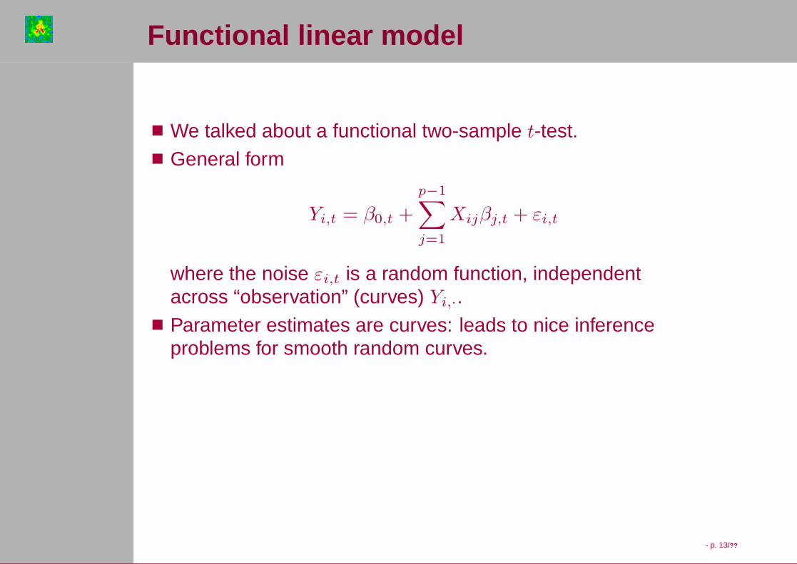
Functional linear model

■ We talked about a functional two-sample t-test.■ General form

Yi,t = β0,t +

p−1∑

j=1

Xijβj,t + εi,t

where the noise εi,t is a random function, independentacross “observation” (curves) Yi,·.

■ Parameter estimates are curves: leads to nice inferenceproblems for smooth random curves.

- p. 14/??

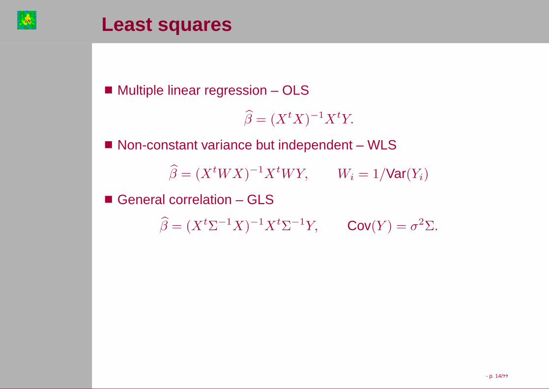
Least squares

■ Multiple linear regression – OLS

β = (XtX)−1XtY.

■ Non-constant variance but independent – WLS

β = (XtWX)−1XtWY, Wi = 1/Var(Yi)

■ General correlation – GLS

β = (XtΣ−1X)−1XtΣ−1Y, Cov(Y ) = σ2Σ.

- p. 15/??

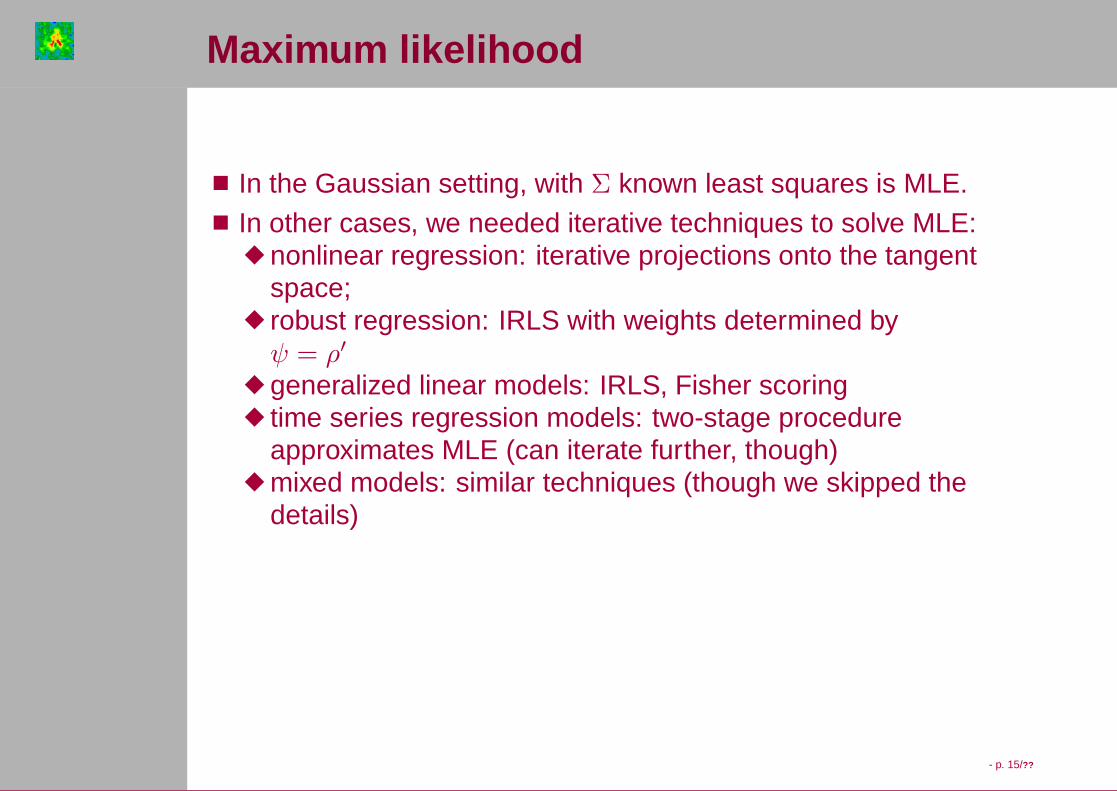
Maximum likelihood

■ In the Gaussian setting, with Σ known least squares is MLE.■ In other cases, we needed iterative techniques to solve MLE:

◆ nonlinear regression: iterative projections onto the tangentspace;

◆ robust regression: IRLS with weights determined byψ = ρ′

◆ generalized linear models: IRLS, Fisher scoring◆ time series regression models: two-stage procedure

approximates MLE (can iterate further, though)◆ mixed models: similar techniques (though we skipped the

details)

- p. 16/??

Diagnostics: influence and outliers

■ Diagnostic plots:◆ Added variable plots.◆ QQplot.◆ Residuals vs. fitted.◆ Standardized residuals vs. fitted.

■ Measures of influence■ Cook’s distance.■ DFFITS.■ DFBETAS.■ Outlier test with Bonferroni correction.■ Techniques are most developed for multiple linear regression

model, but some can be generalized (using “whitened”residuals).

- p. 17/??

Penalized regression

■ We looked at ridge regression, too.■ A generic example of the “bias-variance” tradeoff in statistics.

■ Minimize

SSEλ(β) =

nX

i=1

Yi −

p−1X

j=1

Xijβj

!2

+ λ

p−1X

j=1

β2

j .

■ Other penalties possible: basic idea is that the penalty is ameasure of “complexity” of the model.

■ Smoothing spline: ridge regression for scatterplot smoothers.

- p. 18/??

Hypothesis tests: multiple linear regression

■ Multiple linear regression: model R has j less coefficientsthan model F – equivalently there are j linear constraints onβ’s.

■

F =

SSE(R)−SSE(F )j

SSE(F )n−p

∼ Fj,n−p(if H0 is true)

■ Reject H0 : R is true at level α if F > F1−α,j,n−p.

- p. 19/??

Hypothesis tests: general case

■ Other models: DEV (M) = −2 logL(M) replaces SSE(M).■ Difference D = DEV (R) −DEV (F ) ∼ χ2

j (asymptotically).■ Denominator in the F statistic is usually either known or

based on something like Pearson’s X2:

φ =1

n− p

n∑

i=1

ri(F )2.

In general, residuals are “whitened”

r(M) = Σ(M)−1/2(Y −Xβ(M)).

■ Reject H0 : R is true at level α if D > χ21−α,n−p.

- p. 20/??

Model selection: AIC, BIC, stepwise

■ Best subsets regression (leaps): adjusted R2, Cp.■ Akaike Information Criterion (AIC)

AIC(M) = −2 logL(M) + 2 · p(M).

in model M evaluated at the MLE (Maximum LikelihoodEstimators).

■ Schwarz’s Bayesian Information Criterion (BIC)

BIC(M) = −2 logL(M) + p(M) · log n

■ Penalized regression can be thought of as model selectionas well: choosing the “best” penalty parameter on the basisof

GCV (M) =1

Tr(S(M))

n∑

i=1

(Yi − Yi(M)

)2

whereY (M) = S(M)Y.

- p. 21/??

That’s it!

Thanks!