linear and weighted regression support vector...
TRANSCRIPT
APPLIED MACHINE LEARNING
1
MACHINE LEARNING
Linear and Weighted Regression
Support Vector Regression

APPLIED MACHINE LEARNING
2
How to estimate a continuous output value y?
Color
Len
gth
Bananas
Apples
Maps N-dimensions input x ∈ ℝN to discrete values y
x = [Length, Color] “Banana” or “Apple”
Classification (reminder)
E.g.:

APPLIED MACHINE LEARNING
3
Income: GDP 2003 (log scale)
Life
sat
isfa
ctio
n India
Nigeria
Cambodia
China
US
Japan
Italy
0 10 000 20 000 30 000 40 000
3
4
5
6
7
Bangladesh
Maps N-dimensions input x ∈ ℝN to continuous values y ∈ ℝ
Continuous value of life satisfaction
Regression: introduction
Income (GDP)

APPLIED MACHINE LEARNING
4
Maps N-dimensions input x ∈ ℝN to continuous values y ∈ ℝ
Income (GDP) Continuous value of life satisfaction
Regression: introduction
Income: GDP 2003 (log scale)
Life
sat
isfa
ctio
n India
Nigeria
Cambodia
China
US
Japan
Italy
0 10 000 20 000 30 000 40 000
3
4
5
6
7
Bangladesh
Query point: RussiaGDP = 30 000
Estimation of life satisfaction = 6.5

APPLIED MACHINE LEARNING
5School of Engineering – Section Microtechnique @ 2004 A.. Billard – Adapted from Blei 99 and Dorr & Montz 2004
Example of Use of Regressive MethodsPredict the number of diplomas that will be awarded in the next ten years across
the two EPF the number of diploma follow a non-linear curve as a function of
time.

APPLIED MACHINE LEARNING
6
Example of Use of Regressive MethodsPredict the velocity of the robot given its position.
x*: target
x f x

APPLIED MACHINE LEARNING
7
Example of Use of Regressive Methods

APPLIED MACHINE LEARNING
8
; , Ty f x w b w x b
Linear Regression
Linear regression searches a linear mapping between input x and
output y, parametrized by the slope vector w and intercept b.
y
x
b

APPLIED MACHINE LEARNING
9
; , Ty f x w b w x b
One can omit the intercept by centering the data:
Linear Regression
Linear regression searches a linear mapping between input x and
output y, parametrized by the slope vector w and intercept b.
*
' and ' , , : mean on and
' ' '
with '
Least-square estimate of ' ' ' 0
' '.
T
T
T
T
y y y x x x x y x y
y w x b
b b w x y
b y w x
y w x
APPLIED MACHINE LEARNING
10
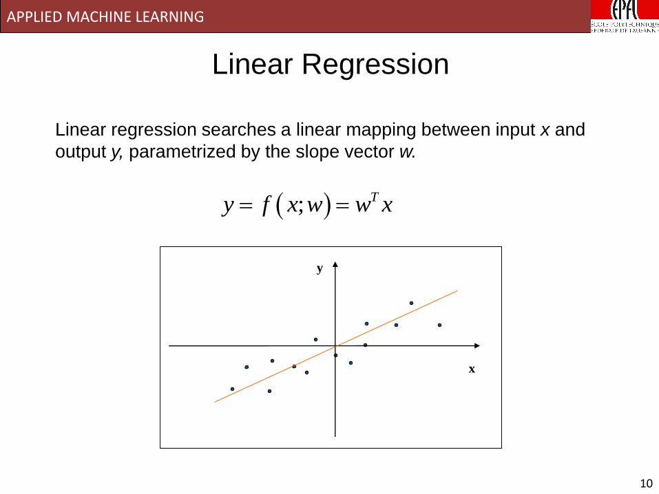
; Ty f x w w x
Linear Regression
Linear regression searches a linear mapping between input x and
output y, parametrized by the slope vector w.
y
x

APPLIED MACHINE LEARNING
11
Linear Regression
1 2 1 2Pair of training points [ ... ] and [ ... ]
, .
M M
i N i
M X x x x y y y y
x y
Find the optimal parameter w through least-square regression:
2
*
1
1min
2i i
MT
wi
w w x y
Finds an analytical solution through partial differentiation:
1
*= T Tw X X X Y
ℝℝ

APPLIED MACHINE LEARNING
12
x
All points have equal weight.
Regression through weighted Least Square
2
*
1 2
1
1min , & ...
2
i ii i
MT
Mw
i
w w x y
Weighted Linear Regression
y
Standard linear regression
ˆ : estimatory
ℝ

APPLIED MACHINE LEARNING
13
y
Points in red have large weights.
Regression through weighted Least Square
2
*
1
1min ,
2
i ii i
MT
wi
w w x y
Weighted Linear Regression
x
y
ℝ

APPLIED MACHINE LEARNING
14
y
Regression through weighted Least Square
Weighted Linear Regression
Points in red have large weights.
x
y
2
*
1
1min ,
2
i ii i
MT
wi
w w x y
ℝ
APPLIED MACHINE LEARNING
15
1
2
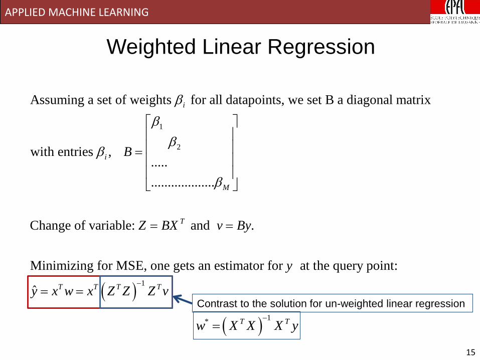
Assuming a set of weights for all datapoints, we set B a diagonal matrix
with entries ,
.....
...................
Change of variable: and .
Minimizing f
i
i
M
T
B
Z BX v By
1
or MSE, one gets an estimator for at the query point:
ˆ T T T T
y
y x w x Z Z Z v
1
* T Tw X X X y
Contrast to the solution for un-weighted linear regression
Weighted Linear Regression

APPLIED MACHINE LEARNING
16
assumes that a single linear dependency applies everywhere.
Not true for data sets with local dependencies.
y
x
Limitations of Linear Regression
2
*
1
1min , : constant weights
2
i ii i
MT
wi
w w x y
Regression through weighted Least Square
ℝ

APPLIED MACHINE LEARNING
17
assumes that a single linear dependency applies everywhere.
Not true for data sets with local dependencies.
It would be useful to design a regression method that estimates best
the linear dependencies locally.
Limitations of Linear Regression
2
*
1
1min , : constant weights
2
i ii i
MT
wi
w w x y
Regression through weighted Least Square
ℝ

APPLIED MACHINE LEARNING
18
Locally Weighted Regression
,
= , , with , , , .i
i i i id x x
i x K d x x K d x x e d x x x x
y x
X: query point
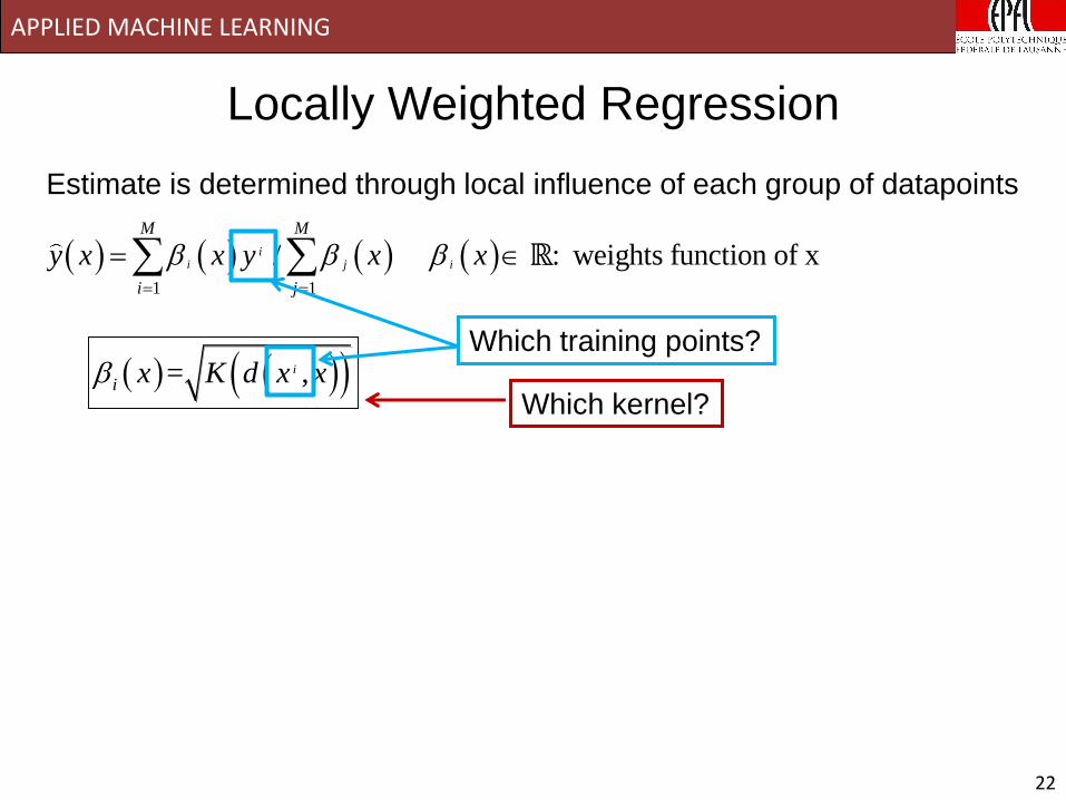
Estimate is determined through local influence of each group of datapoints
1 1
/ : weights function of xii j i
M M
i j
y x x y x x
y
ℝ

APPLIED MACHINE LEARNING
19
Locally Weighted Regression
,
= , , with , , , .i
i i i id x x
i x K d x x K d x x e d x x x x
Estimate is determined through local influence of each group of datapoints
X: query point
y x
Generates a smooth function y(x)
1 1
/ : weights function of xii j i
M M
i j
y x x y x x
y
ℝ

APPLIED MACHINE LEARNING
20
Locally Weighted Regression
Estimate is determined through local influence of each group of datapoints
1 1
/ : weights function of xii j i
M M
i j
y x x y x x
Model-free regression!
No longer explicit model of the formTy w x
Regression computed at each query point.
Depends on training points.
= ,i
i x K d x x
ℝ

APPLIED MACHINE LEARNING
21
Locally Weighted Regression
1 1
/ : weights function of xii j i
M M
i j
y x x y x x
Estimate is determined through local influence of each group of datapoints
2
1
ˆmin min ,
Local cost function at , the query point.
i i
M
i
J x y y K d x x
x
Optimal solution to the local cost function:
= ,i
i x K d x x
ℝ
APPLIED MACHINE LEARNING
22
= ,i
i x K d x x
Locally Weighted Regression
Estimate is determined through local influence of each group of datapoints
1 1
/ : weights function of xii j i
M M
i j
y x x y x x
Which training points?
Which kernel?
ℝ

APPLIED MACHINE LEARNING
23
Exercise Session Part I
APPLIED MACHINE LEARNING
24
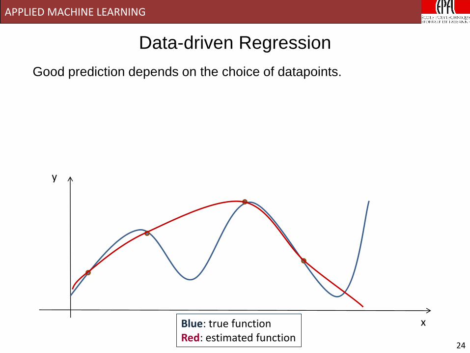
Data-driven Regression
y
xBlue: true functionRed: estimated function
Good prediction depends on the choice of datapoints.

APPLIED MACHINE LEARNING
25
y
Good prediction depends on the choice of datapoints.
The more datapoints, the better the fit.
Computational costs increase dramatically with number of datapoints
x
Data-driven Regression
Blue: true functionRed: estimated function

APPLIED MACHINE LEARNING
26
y
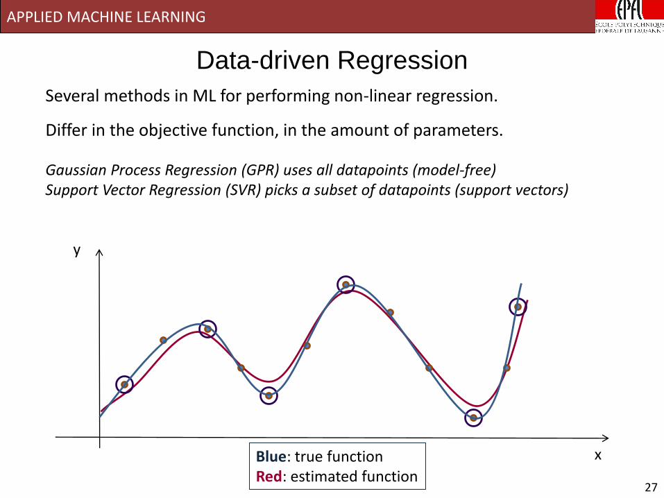
Several methods in ML for performing non-linear regression.
Differ in the objective function, in the amount of parameters.
Gaussian Process Regression (GPR) uses all datapoints (model-free)
x
Data-driven Regression
Gaussian Process Regression not covered in class!Not examined in the final exam!
Blue: true functionRed: estimated function
APPLIED MACHINE LEARNING
27
y
Several methods in ML for performing non-linear regression.
Differ in the objective function, in the amount of parameters.
Gaussian Process Regression (GPR) uses all datapoints (model-free) Support Vector Regression (SVR) picks a subset of datapoints (support vectors)
x
Data-driven Regression
Blue: true functionRed: estimated function

APPLIED MACHINE LEARNING
28
y
x
Several methods in ML for performing non-linear regression.
Differ in the objective function, in the amount of parameters.
Gaussian Process Regression (GPR) uses all datapoints (model-free) Support Vector Regression (SVR) picks a subset of datapoints (support vectors)Gaussian Mixture Regression (GMR) generates a new set of datapoints (centers of Gaussian functions)
Data-driven Regression
Blue: true functionRed: estimated function

APPLIED MACHINE LEARNING
29
y
x
Data-driven Regression
Estimate of the noise is important to measure goodness of fit.

APPLIED MACHINE LEARNING
31
y
x
Support Vector Regression (SVR) assumes an estimate of the noise
model (e-tube) and then compute f directly within a noise-tolerance.
Estimate of the noise is important to measure goodness of fit.
Data-driven Regression

APPLIED MACHINE LEARNING
32
y
x
Gaussian Mixture Regression (GMR) builds a local estimate of the noise
model through the variance of the system.
Estimate of the noise is important to measure goodness of fit.
Data-driven Regression

APPLIED MACHINE LEARNING
33
Support Vector Regression

APPLIED MACHINE LEARNING
34
1,...
Assume a nonlinear mapping , s.t. .
How to estimate to best predict the pair of training points , ?i i
i M
f y f x
f x y
How to generalize the support vector machine framework for classification to estimate continuous functions?
1. Assume a non-linear mapping through feature space and then perform linear regression in feature space
2. Supervised learning – minimizes an error function.
First determine a way to measure error on testing set in the linear case!
Support Vector Regression

APPLIED MACHINE LEARNING
35
Assume a linear mapping , s.t. .Tf y f x w x b
Measure the error on prediction
b is estimated as in SVR through least-square regression on support vectors; hence we ignore it for the rest of the developments .
Support Vector Regression
1,...
How to estimate and to best predict the pair of training points , ?i i
i Mw b x y
x
y Ty f x w x b

APPLIED MACHINE LEARNING
36
Support Vector Regression
Set an upper bound on the error and
consider as correctly classified all points
such that ( ) ,
Penalize only datapoints that are
not contained in the -tube.
f x y
e
e
e
x
y Ty f x w x b

APPLIED MACHINE LEARNING
37
x
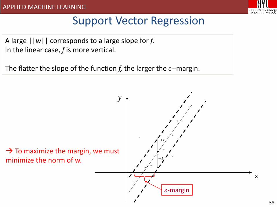
Support Vector Regression
e-margin
The e-margin is a measure of the width of the e-insensitive tube.It is a measure of the precision of the regression.
A small ||w|| corresponds to a small slope for f. In the linear case, f is more horizontal.
y
APPLIED MACHINE LEARNING
38
x
Support Vector Regression
e-margin
y
A large ||w|| corresponds to a large slope for f. In the linear case, f is more vertical.
The flatter the slope of the function f, the larger the emargin.
To maximize the margin, we must minimize the norm of w.

APPLIED MACHINE LEARNING
41
Support Vector Regression
2
1,...
This can be rephrased as a constraint-based optimization problem
of the form:
1minimize
2
,subject to
,
i
i
i
i
i M
w
w x b y
y w x b
e
e
Need to penalize points outside the e-insensitive tube.

APPLIED MACHINE LEARNING
42
Support Vector Regression
Need to penalize points outside the e-insensitive tube.
*
2 *
1
*
*
Introduce slack variables , , 0 :
1 Cminimize +
2
,
subject to ,
0, 0
i
i
i i
M
i i
i
i
i
i
i
i i
C
wM
w x b y
y w x b
e
e
i*
i

APPLIED MACHINE LEARNING
43
Support Vector Regression
All points outside the e-tube become Support Vectors
i*
i
*
2 *
1
*
*
Introduce slack variables , , 0 :
1 Cminimize +
2
,
subject to ,
0, 0
i
i
i i
M
i i
i
i
i
i
i
i i
C
wM
w x b y
y w x b
e
e
We now have the solution to the linear regression problem.
How to generalize this to the nonlinear case?

APPLIED MACHINE LEARNING
44
Lift x into feature space and then perform linear regression in feature space.
Linear Case:
,
Non-Linear Case:
,
y f x w x b
x x
y f x w x b
w lives in feature space!
x x
Support Vector Regression

APPLIED MACHINE LEARNING
45
Support Vector Regression
2 *
1
*
*
In feature space, we obtain the same constrained optimization problem:
1 Cminimize +
2
,
subject to ,
0, 0
i
i
M
i i
i
i
i
i
i
i i
wM
w x b y
y w x b
e
e

APPLIED MACHINE LEARNING
46
Support Vector Regression
2 * * *
1 1
1
* *
1
1 C CL , , *, = +
2
,
,
i
ii
i
i
M M
i i i i i
i i
Mi
i
i
Mi
i
i
w b wM M
y w x b
y w x b
e
e
Again, we can solve this quadratic problem by introducing sets of
Lagrange multipliers and writing the Lagrangian :
Lagrangian = Objective function + l * constraints

APPLIED MACHINE LEARNING
47
2 * * *
1 1
1
* *
1
1 C CL , , *, = +
2
,
,
i
ii
i
i
M M
i i i i i
i i
Mi
i
i
Mi
i
i
w b wM M
y w x b
y w x b
e
e
Support Vector Regression
i*
i
Constraints on points lying on either side of the e-tube
* & 0 for all points that do not satisfy the constraints
points outside the -tube
ii
e
0i
* 0i

APPLIED MACHINE LEARNING
48
Support Vector Regression
0i
* 0i
Requiring that the partial derivatives are all zero:
*
1
L0.i
Mi
i
i
w xw
*
1
.i
Mi
i
i
w x
Linear combination of support vectors
*
1
L0.i
M
i
ib
*
1 1
i
M M
i
i i
Rebalancing the effect of the support vectors on both sides of the e-tube
* & 0 for all points that do not satisfy the constraints
points outside the -tube
ii
e
APPLIED MACHINE LEARNING
49
*
* *
, 1
* *,
1 1
* *
1
1,
2max
subject to 0 and , 0,
i
i i
i i
Mi j
i j j
i j
M Mi
i i
i i
Mi
i i
i
x x
y
C
M
e
Support Vector Regression
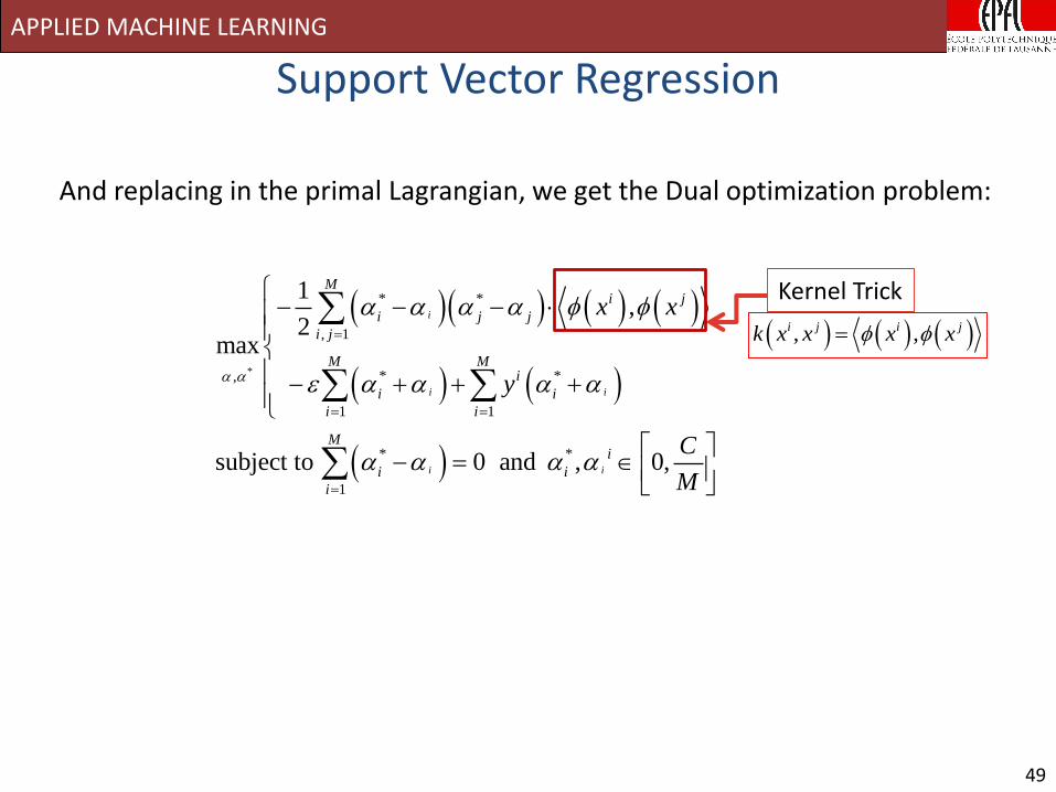
And replacing in the primal Lagrangian, we get the Dual optimization problem:
, ,i j i jk x x x x
Kernel Trick

APPLIED MACHINE LEARNING
50
Support Vector Regression
The solution is given by:
*
1
,i
Mi
i
i
y f x k x x b
Linear Coefficients(Lagrange multipliers for each constraint).
If one uses RBF Kernel,M un-normalized isotropic Gaussians centered on each training datapoint.
*
1
, ,i
Mi
i
i
y f x w x b x x b
, ,i j i jk x x x x
Kernel Trick

APPLIED MACHINE LEARNING
51
Support Vector Regression
y
x
*
1
,i
Mi
i
i
y f x k x x b
The solution is given by:
Kernel places a Gauss function on each SV

APPLIED MACHINE LEARNING
52
Support Vector Regression
y
x
*
1
,i
Mi
i
i
y f x k x x b
The solution is given by:
The Lagrange multipliers define the importance of each Gaussian function.
*
1 1.5 2 2 4 3 *
3 1.5 *
5 1 6 2.5
b
Converges to b when SV effect vanishes.
1x 2x 3x 4x 5x6x
Y=f(x)

APPLIED MACHINE LEARNING
53
*
1
*
1 1
SVR gives the following estimate for each pair of datapoints ,
, , i 1...
An estimate of can be computed using the above:
1,
j j
Mj j i
i i
i
M Mj j i
i i
j i
y x
y k x x b M
b
b y k x xM
Support Vector Regression
APPLIED MACHINE LEARNING
54
2 *
1
*
*
1 Cminimize +
2
,
subject to ,
0, 0
i
i
M
i i
i
i
i
i
i
i i
wM
w x b y
y w x b
e
e
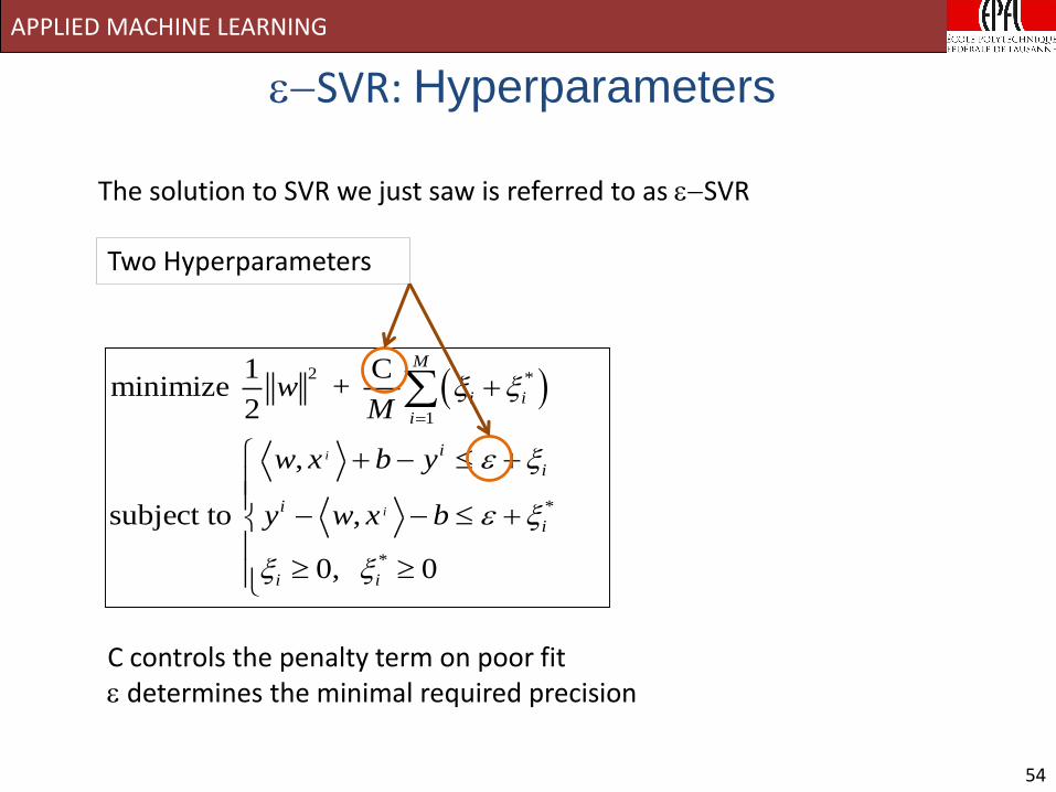
eSVR: Hyperparameters
The solution to SVR we just saw is referred to as eSVR
Two Hyperparameters
C controls the penalty term on poor fite determines the minimal required precision

APPLIED MACHINE LEARNING
55
Effect of the RBF kernel width on the fit. Here fit using C=100, e=0.1, kernel width=0.01.
eSVR: Effect of Hyperparameters

APPLIED MACHINE LEARNING
56
Effect of the RBF kernel width on the fit. Here fit using C=100, e=0.01, kernel width=0.01
eSVR: Effect of Hyperparameters
Overfitting

APPLIED MACHINE LEARNING
57
eSVR: Effect of Hyperparameters
Effect of the RBF kernel width on the fit. Here fit using C=100, e=0.05, kernel width=0.01 Reduction of the effect of the kernel width on the fit by choosing appropriate hyperparameters..

APPLIED MACHINE LEARNING
58
eSVR: Effect of Hyperparameters
Mldemos does not display the support vectors if there is more than one point for the same x!
APPLIED MACHINE LEARNING
59
Summary
Linear regression can be solved through Least-Mean-Square
estimation and yields an optimal analytical solution.
Weighted regression offers the possibility to perform a local
regression and yields also an optimal analytical solution.
The estimate is no longer global and is computed around each
group of data point!
Support Vector Regression: performs regression on a non-linear
function. Determines automatically the important points. The
estimate is globally optimal.

APPLIED MACHINE LEARNING
60
Examples of Applications of SVR Next
APPLIED MACHINE LEARNING
61
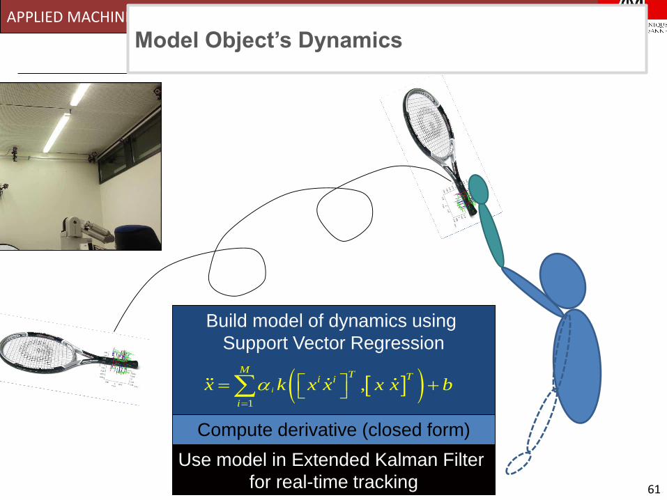
Catching Objects in FlightModel Object’s Dynamics
Build model of dynamics using
Support Vector Regression
Compute derivative (closed form)
Use model in Extended Kalman Filter
for real-time tracking
1
, i
MT Ti i
i
x k x x x x b
APPLIED MACHINE LEARNING
62
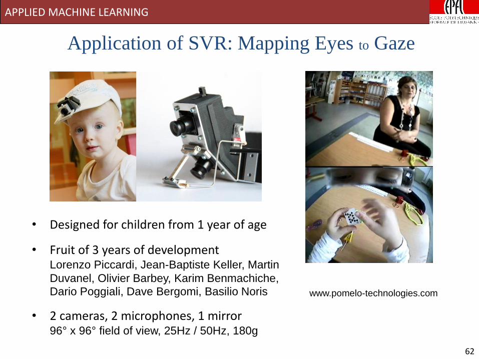
• Designed for children from 1 year of age
• Fruit of 3 years of developmentLorenzo Piccardi, Jean-Baptiste Keller, Martin
Duvanel, Olivier Barbey, Karim Benmachiche, Dario Poggiali, Dave Bergomi, Basilio Noris
• 2 cameras, 2 microphones, 1 mirror96° x 96° field of view, 25Hz / 50Hz, 180g
www.pomelo-technologies.com
Application of SVR: Mapping Eyes to Gaze

APPLIED MACHINE LEARNING
63
B. Noris, J.-B. Keller and A. Billard. A Wearable Gaze Tracking System for Children in Unconstrained Environments. Int. journal of Computer Vision and
Image Understanding, 2011
Application of SVR: Mapping Eyes to Gaze

APPLIED MACHINE LEARNING
64
96°
96°
Application of SVR: Mapping Eyes to Gaze

APPLIED MACHINE LEARNING
65
Use Support Vector Regression to learn the mapping from eyes
appearance to gaze coordinates.
?
Application of SVR: Mapping Eyes to Gaze

APPLIED MACHINE LEARNING
66
We normalize the image through high-pass filtering
We collect images of the eyes and directions of the gaze.
+ + + + ...
Learn mapping Eye Image Position in Image through
Support Vector Regression (SVR)
Application of SVR: Mapping Eyes to Gaze
APPLIED MACHINE LEARNING
67
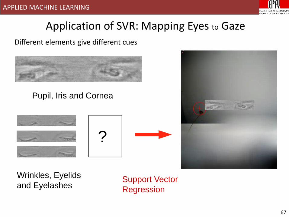
Different elements give different cues
Pupil, Iris and Cornea
?
Wrinkles, Eyelids
and EyelashesSupport Vector
Regression
Application of SVR: Mapping Eyes to Gaze
APPLIED MACHINE LEARNING
68
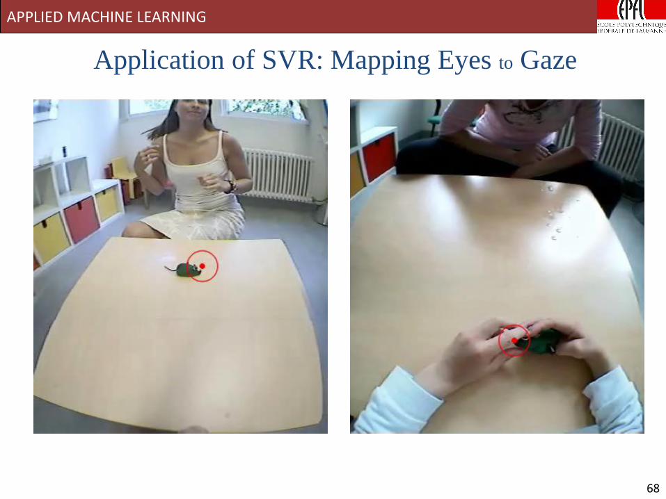
Application of SVR: Mapping Eyes to Gaze

APPLIED MACHINE LEARNING
69
From
object recognition using
Eye tracking
To reconstructing path
in Shop
www.pomelo-technologies.com

APPLIED MACHINE LEARNING
70
Gaze tracking using SVR Object detection using SVM
Monitoring Consumers’ Visual Behavior

APPLIED MACHINE LEARNING
71
Msc Projects in Industry