lind−marchal−wathen: © the mcgraw−hill … vol. 16, no. 43.) hypothesis testinga procedure...
TRANSCRIPT

Lind−Marchal−Wathen: Statistical Techniques in Business and Economics, 13th Edition
10. One−Sample Tests of Hypothesis
Text © The McGraw−Hill Companies, 2008
10G O A L SWhen you have completedthis chapter you will beable to:
1 Define a hypothesis andhypothesis testing.
2 Describe the five-stephypothesis-testing procedure.
3 Distinguish between aone-tailed and a two-tailedtest of hypothesis.
4 Conduct a test of hypothesisabout a population mean.
5 Conduct a test of hypothesisabout a population proportion.
6 Define Type I and Type IIerrors.
7 Compute the probability ofa Type II error.
One-Sample Testsof Hypothesis
According to the Coffee Research Organization the typical American
coffee drinker consumes an average of 3.1 cups per day. A sample
of 12 senior citizens reported the amounts of coffee in cups
consumed in a particular day. At the .05 significance level does the
sample data provided in the exercise suggest a difference between
the national average and the sample mean from senior citizens.
(See Exercise 39, Goal 4.)
Lind−Marchal−Wathen: Statistical Techniques in Business and Economics, 13th Edition
10. One−Sample Tests of Hypothesis
Text © The McGraw−Hill Companies, 2008
One-Sample Tests of Hypothesis 331
IntroductionChapter 8 began our study of statistical inference. We described how we couldselect a random sample and from this sample estimate the value of a populationparameter. For example, we selected a sample of 5 employees at Spence Sprockets,found the number of years of service for each sampled employee, computed themean years of service, and used the sample mean to estimate the mean years ofservice for all employees. In other words, we estimated a population parameter froma sample statistic.
Chapter 9 continued the study of statistical inference by developing a confi-dence interval. A confidence interval is a range of values within which we expectthe population parameter to occur. In this chapter, rather than develop a range ofvalues within which we expect the population parameter to occur, we develop aprocedure to test the validity of a statement about a population parameter. Someexamples of statements we might want to test are:
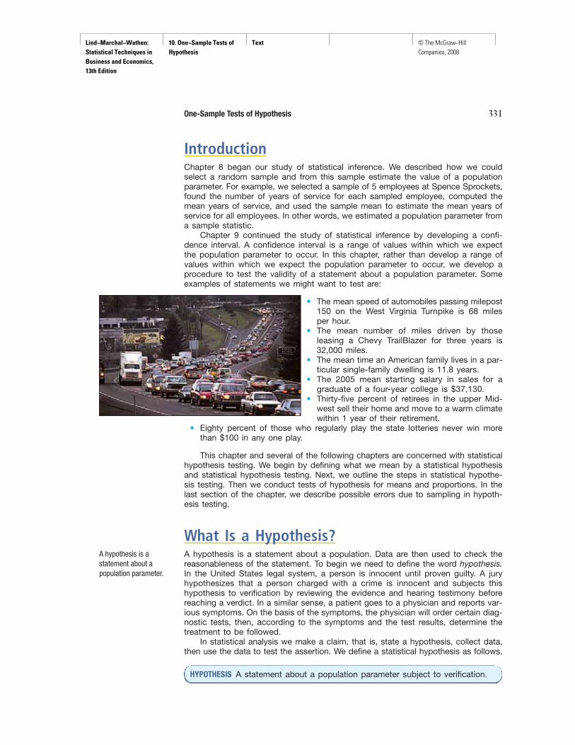
• The mean speed of automobiles passing milepost150 on the West Virginia Turnpike is 68 milesper hour.
• The mean number of miles driven by thoseleasing a Chevy TrailBlazer for three years is32,000 miles.
• The mean time an American family lives in a par-ticular single-family dwelling is 11.8 years.
• The 2005 mean starting salary in sales for agraduate of a four-year college is $37,130.
• Thirty-five percent of retirees in the upper Mid-west sell their home and move to a warm climatewithin 1 year of their retirement.
• Eighty percent of those who regularly play the state lotteries never win morethan $100 in any one play.
This chapter and several of the following chapters are concerned with statisticalhypothesis testing. We begin by defining what we mean by a statistical hypothesisand statistical hypothesis testing. Next, we outline the steps in statistical hypothe-sis testing. Then we conduct tests of hypothesis for means and proportions. In thelast section of the chapter, we describe possible errors due to sampling in hypoth-esis testing.
What Is a Hypothesis?A hypothesis is a statement about a population. Data are then used to check thereasonableness of the statement. To begin we need to define the word hypothesis.In the United States legal system, a person is innocent until proven guilty. A juryhypothesizes that a person charged with a crime is innocent and subjects thishypothesis to verification by reviewing the evidence and hearing testimony beforereaching a verdict. In a similar sense, a patient goes to a physician and reports var-ious symptoms. On the basis of the symptoms, the physician will order certain diag-nostic tests, then, according to the symptoms and the test results, determine thetreatment to be followed.
In statistical analysis we make a claim, that is, state a hypothesis, collect data,then use the data to test the assertion. We define a statistical hypothesis as follows.
A hypothesis is astatement about apopulation parameter.
HYPOTHESIS A statement about a population parameter subject to verification.

Lind−Marchal−Wathen: Statistical Techniques in Business and Economics, 13th Edition
10. One−Sample Tests of Hypothesis
Text © The McGraw−Hill Companies, 2008
In most cases the population is so large that it is not feasible to study all the items,objects, or persons in the population. For example, it would not be possible tocontact every systems analyst in the United States to find his or her monthlyincome. Likewise, the quality assurance department at Cooper Tire cannot checkeach tire produced to determine whether it will last more than 60,000 miles.
As noted in Chapter 8, an alternative to measuring or interviewing the entirepopulation is to take a sample from the population. We can, therefore, test a state-ment to determine whether the sample does or does not support the statement con-cerning the population.
What Is Hypothesis Testing?The terms hypothesis testing and testing a hypothesis are used interchangeably.Hypothesis testing starts with a statement, or assumption, about a populationparameter—such as the population mean. As noted, this statement is referred toas a hypothesis. A hypothesis might be that the mean monthly commission ofsales associates in retail electronics stores, such as Circuit City, is $2,000. Wecannot contact all these sales associates to ascertain that the mean is in fact$2,000. The cost of locating and interviewing every electronics sales associatein the United States would be exorbitant. To test the validity of the assumption(� � $2,000), we must select a sample from the population of all electronicssales associates, calculate sample statistics, and based on certain decisionrules accept or reject the hypothesis. A sample mean of $1,000 for the electron-ics sales associates would certainly cause rejection of the hypothesis. However,suppose the sample mean is $1,995. Is that close enough to $2,000 for us toaccept the assumption that the population mean is $2,000? Can we attribute thedifference of $5 between the two means to sampling error, or is that differencestatistically significant?
332 Chapter 10
Statistics in Action
LASIK is a 15-minutesurgical procedure thatuses a laser to reshapean eye’s cornea with thegoal of improving eye-sight. Research showsthat about 5 percentof all surgeries involvecomplications suchas glare, corneal haze,over-correction orunder-correction ofvision, and loss ofvision. In a statisticalsense, the research testsa null hypothesis thatthe surgery will notimprove eyesight withthe alternative hypothe-sis that the surgery willimprove eyesight. Thesample data of LASIKsurgery shows that 5 per-cent of all cases resultin complications. The5 percent represents aType I error rate. Whena person decides to havethe surgery, he or she ex-pects to reject the nullhypothesis. In 5 percentof future cases, this ex-pectation will not bemet. (Source: AmericanAcademy of Ophthal-mology Journal, SanFrancisco, Vol. 16,no. 43.)
HYPOTHESIS TESTING A procedure based on sample evidence and probabilitytheory to determine whether the hypothesis is a reasonable statement.
Five-Step Procedure for Testing a HypothesisThere is a five-step procedure that systematizes hypothesis testing; when we getto step 5, we are ready to reject or not reject the hypothesis. However, hypothe-sis testing as used by statisticians does not provide proof that something is true,in the manner in which a mathematician “proves” a statement. It does provide akind of “proof beyond a reasonable doubt,” in the manner of the court system.Hence, there are specific rules of evidence, or procedures, that are followed. Thesteps are shown in the following diagram. We will discuss in detail each of thesteps.
Step 1 Step 2 Step 3 Step 4 Step 5 Do notreject H0
orreject H0
andaccept H1
Take a sample,arrive atdecision
Formulate adecision
rule
Select alevel of
significance
Identify thetest
statistic
State null andalternate
hypotheses

Lind−Marchal−Wathen: Statistical Techniques in Business and Economics, 13th Edition
10. One−Sample Tests of Hypothesis
Text © The McGraw−Hill Companies, 2008
One-Sample Tests of Hypothesis 333
Step 1: State the Null Hypothesis (H0) and theAlternate Hypothesis (H1)The first step is to state the hypothesis being tested. It is called the null hypothesis,designated H0, and read “H sub zero.” The capital letter H stands for hypothesis,and the subscript zero implies “no difference.” There is usually a “not” or a “no” termin the null hypothesis, meaning that there is “no change.” For example, the nullhypothesis is that the mean number of miles driven on the steel-belted tire is not dif-ferent from 60,000. The null hypothesis would be written H0: � � 60,000. Generallyspeaking, the null hypothesis is developed for the purpose of testing. We either rejector fail to reject the null hypothesis. The null hypothesis is a statement that is notrejected unless our sample data provide convincing evidence that it is false.
We should emphasize that, if the null hypothesis is not rejected on the basis ofthe sample data, we cannot say that the null hypothesis is true. To put it anotherway, failing to reject the null hypothesis does not prove that H0 is true, it means wehave failed to disprove H0. To prove without any doubt the null hypothesis is true,the population parameter would have to be known. To actually determine it, wewould have to test, survey, or count every item in the population. This is usually notfeasible. The alternative is to take a sample from the population.
It should also be noted that we often begin the null hypothesis by stating, “Thereis no significant difference between . . . ,” or “The mean impact strength of the glassis not significantly different from . . .” When we select a sample from a population,the sample statistic is usually numerically different from the hypothesized populationparameter. As an illustration, suppose the hypothesized impact strength of a glassplate is 70 psi, and the mean impact strength of a sample of 12 glass plates is 69.5psi. We must make a decision about the difference of 0.5 psi. Is it a true difference,that is, a significant difference, or is the difference between the sample statistic (69.5)and the hypothesized population parameter (70.0) due to chance (sampling)? Asnoted, to answer this question we conduct a test of significance, commonly referredto as a test of hypothesis. To define what is meant by a null hypothesis:
State the null hypothesisand the alternativehypothesis.
NULL HYPOTHESIS A statement about the value of a population parameterdeveloped for the purpose of testing numerical evidence.
ALTERNATE HYPOTHESIS A statement that is accepted if the sample data providesufficient evidence that the null hypothesis is false.
The alternate hypothesis describes what you will conclude if you reject thenull hypothesis. It is written H1 and is read “H sub one.” It is also referred to as theresearch hypothesis. The alternate hypothesis is accepted if the sample data provideus with enough statistical evidence that the null hypothesis is false.
Five-step systematicprocedure
The following example will help clarify what is meant by the null hypothesis andthe alternate hypothesis. A recent article indicated the mean age of U.S. commer-cial aircraft is 15 years. To conduct a statistical test regarding this statement, thefirst step is to determine the null and the alternate hypotheses. The null hypothesisrepresents the current or reported condition. It is written H0: � � 15. The alternatehypothesis is that the statement is not true, that is, H1: � � 15. It is important toremember that no matter how the problem is stated, the null hypothesis will alwayscontain the equal sign. The equal sign (�) will never appear in the alternate hypoth-esis. Why? Because the null hypothesis is the statement being tested, and we needa specific value to include in our calculations. We turn to the alternate hypothesisonly if the data suggests the null hypothesis is untrue.

Lind−Marchal−Wathen: Statistical Techniques in Business and Economics, 13th Edition
10. One−Sample Tests of Hypothesis
Text © The McGraw−Hill Companies, 2008
Step 2: Select a Level of SignificanceAfter setting up the null hypothesis and alternate hypothesis, the next step is tostate the level of significance.
334 Chapter 10
Select a level ofsignificance or risk.
LEVEL OF SIGNIFICANCE The probability of rejecting the null hypothesis when itis true.
The level of significance is designated �, the Greek letter alpha. It is also some-times called the level of risk. This may be a more appropriate term because it is therisk you take of rejecting the null hypothesis when it is really true.
There is no one level of significance that is applied to all tests. A decision ismade to use the .05 level (often stated as the 5 percent level), the .01 level, the .10level, or any other level between 0 and 1. Traditionally, the .05 level is selected forconsumer research projects, .01 for quality assurance, and .10 for political polling.You, the researcher, must decide on the level of significance before formulating adecision rule and collecting sample data.
To illustrate how it is possible to reject a true hypothesis, suppose a firm manu-facturing personal computers uses a large number of printed circuit boards. Suppliers
bid on the boards, and the one with the lowest bid isawarded a sizable contract. Suppose the contractspecifies that the computer manufacturer’s quality-assurance department will sample all incoming ship-ments of circuit boards. If more than 6 percent of theboards sampled are substandard, the shipment will berejected. The null hypothesis is that the incoming ship-ment of boards contains 6 percent or less substan-dard boards. The alternate hypothesis is that morethan 6 percent of the boards are defective.
A sample of 50 circuit boards received July 21from Allied Electronics revealed that 4 boards, or 8 per-cent, were substandard. The shipment was rejectedbecause it exceeded the maximum of 6 percent sub-standard printed circuit boards. If the shipment wasactually substandard, then the decision to return theboards to the supplier was correct. However, suppose
the 4 substandard printed circuit boards selected in the sample of 50 were the onlysubstandard boards in the shipment of 4,000 boards. Then only 1�10 of 1 percent weredefective (4�4,000 � .001). In that case, less than 6 percent of the entire shipmentwas substandard and rejecting the shipment was an error. In terms of hypothesis test-ing, we rejected the null hypothesis that the shipment was not substandard whenwe should have accepted the null hypothesis. By rejecting a true null hypothesis, wecommitted a Type I error. The probability of committing a Type I error is �.
TYPE I ERROR Rejecting the null hypothesis, H0, when it is true.
The probability of committing another type of error, called a Type II error, is des-ignated by the Greek letter beta (�).
TYPE II ERROR Accepting the null hypothesis when it is false.
The firm manufacturing personal computers would commit a Type II error if,unknown to the manufacturer, an incoming shipment of printed circuit boards fromAllied Electronics contained 15 percent substandard boards, yet the shipment

Lind−Marchal−Wathen: Statistical Techniques in Business and Economics, 13th Edition
10. One−Sample Tests of Hypothesis
Text © The McGraw−Hill Companies, 2008
One-Sample Tests of Hypothesis 335
Researcher
Null Does Not Reject RejectsHypothesis H0 H0
H0 is trueCorrect Type Idecision error
H0 is falseType II Correcterror decision
was accepted. How could this happen? Suppose 2 of the 50 boards in the sample(4 percent) tested were substandard, and 48 of the 50 were good boards. Accord-ing to the stated procedure, because the sample contained less than 6 percent sub-standard boards, the shipment was accepted. It could be that by chance the 48good boards selected in the sample were the only acceptable ones in the entireshipment consisting of thousands of boards!
In retrospect, the researcher cannot study every item or individual in the pop-ulation. Thus, there is a possibility of two types of error—a Type I error, wherein thenull hypothesis is rejected when it should have been accepted, and a Type II error,wherein the null hypothesis is not rejected when it should have been rejected.
We often refer to the probability of these two possible errors as alpha, �, andbeta, �. Alpha (�) is the probability of making a Type I error, and beta (�) is the prob-ability of making a Type II error.
The following table summarizes the decisions the researcher could make andthe possible consequences.
Step 3: Select the Test StatisticThere are many test statistics. In this chapter we use both z and t as the test sta-tistic. In other chapters we will use such test statistics as F and �2, called chi-square.
TEST STATISTIC A value, determined from sample information, used to determinewhether to reject the null hypothesis.
In hypothesis testing for the mean (�) when � is known, the test statistic z is com-puted by:
TESTING A MEAN, � KNOWN [10–1]z �X �
�1n
The z value is based on the sampling distribution of which follows the normaldistribution with a mean equal to �, and a standard deviation , which is equal to . We can thus determine whether the difference between and � isstatistically significant by finding the number of standard deviations is from �,using formula (10–1).
Step 4: Formulate the Decision RuleA decision rule is a statement of the specific conditions under which the null hypoth-esis is rejected and the conditions under which it is not rejected. The region or areaof rejection defines the location of all those values that are so large or so small thatthe probability of their occurrence under a true null hypothesis is rather remote.
Chart 10–1 portrays the rejection region for a test of significance that will beconducted later in the chapter.
XX��1n
�x(�x )X,
The decision rule statesthe conditions when H0is rejected.

Lind−Marchal−Wathen: Statistical Techniques in Business and Economics, 13th Edition
10. One−Sample Tests of Hypothesis
Text © The McGraw−Hill Companies, 2008
336 Chapter 10
Scale of z0 1.65Criticalvalue
Region of rejection
Do notreject Ho
Probability = .95 Probability = .05
CHART 10–1 Sampling Distribution of the Statistic z, a Right-Tailed Test, .05 Level of Significance
Note in the chart that:
1. The area where the null hypothesis is not rejected is to the left of 1.65. We willexplain how to get the 1.65 value shortly.
2. The area of rejection is to the right of 1.65.3. A one-tailed test is being applied. (This will also be explained later.)4. The .05 level of significance was chosen.5. The sampling distribution of the statistic z follows the normal probability
distribution.6. The value 1.65 separates the regions where the null hypothesis is rejected and
where it is not rejected.7. The value 1.65 is the critical value.
Statistics in Action
During World War II,allied military plan-ners needed estimatesof the number ofGerman tanks. Theinformation providedby traditional spyingmethods was not reli-able, but statisticalmethods proved to bevaluable. For exam-ple, espionage andreconnaissance ledanalysts to estimatethat 1,550 tanks wereproduced duringJune 1941. However,using the serialnumbers of capturedtanks and statisticalanalysis, militaryplanners estimated244. The actual num-ber produced, asdetermined fromGerman productionrecords, was 271. Theestimate using statisti-cal analysis turnedout to be much moreaccurate. A similartype of analysis wasused to estimate thenumber of Iraqi tanksdestroyed duringDesert Storm.
CRITICAL VALUE The dividing point between the region where the null hypothesisis rejected and the region where it is not rejected.
Step 5: Make a DecisionThe fifth and final step in hypothesis testing is computing the test statistic, com-paring it to the critical value, and making a decision to reject or not to reject the nullhypothesis. Referring to Chart 10–1, if, based on sample information, z is computedto be 2.34, the null hypothesis is rejected at the .05 level of significance. Thedecision to reject H0 was made because 2.34 lies in the region of rejection, that is,beyond 1.65. We would reject the null hypothesis, reasoning that it is highly improb-able that a computed z value this large is due to sampling error (chance).
Had the computed value been 1.65 or less, say 0.71, the null hypothesis wouldnot be rejected. It would be reasoned that such a small computed value could beattributed to chance, that is, sampling error.
As noted, only one of two decisions is possible in hypothesis testing—eitheraccept or reject the null hypothesis. Instead of “accepting” the null hypothesis, H0,some researchers prefer to phrase the decision as: “Do not reject H0,” “We fail toreject H0,” or “The sample results do not allow us to reject H0.”
It should be reemphasized that there is always a possibility that the null hypothe-sis is rejected when it should not be rejected (a Type I error). Also, there is a definablechance that the null hypothesis is accepted when it should be rejected (a Type II error).

Lind−Marchal−Wathen: Statistical Techniques in Business and Economics, 13th Edition
10. One−Sample Tests of Hypothesis
Text © The McGraw−Hill Companies, 2008
One-Sample Tests of Hypothesis 337
SUMMARY OF THE STEPS IN HYPOTHESIS TESTING1. Establish the null hypothesis (H0 ) and the alternate hypothesis (H1).2. Select the level of significance, that is �.3. Select an appropriate test statistic.4. Formulate a decision rule based on steps 1, 2, and 3 above.5. Make a decision regarding the null hypothesis based on the sample infor-
mation. Interpret the results of the test.
One-Tailed and Two-Tailed Tests of SignificanceRefer to Chart 10–1. It depicts a one-tailed test. The region of rejection is only inthe right (upper) tail of the curve. To illustrate, suppose that the packaging depart-ment at General Foods Corporation is concerned that some boxes of Grape Nutsare significantly overweight. The cereal is packaged in 453-gram boxes, so the nullhypothesis is H0: � � 453. This is read, “the population mean (�) is equal to or lessthan 453.” The alternate hypothesis is, therefore, H1: � � 453. This is read, “� isgreater than 453.” Note that the inequality sign in the alternate hypothesis (�) pointsto the region of rejection in the upper tail. (See Chart 10–1.) Also note that the nullhypothesis includes the equal sign. That is, H0: � � 453. The equality conditionalways appears in H0, never in H1.
Chart 10–2 portrays a situation where the rejection region is in the left (lower) tailof the normal distribution. As an illustration, consider the problem of automobile man-ufacturers, large automobile leasing companies, and other organizations that purchaselarge quantities of tires. They want the tires to average, say, 60,000 miles of wear undernormal usage. They will, therefore, reject a shipment of tires if tests reveal that themean life of the tires is significantly below 60,000 miles. They gladly accept a shipmentif the mean life is greater than 60,000 miles! They are not concerned with this possi-bility, however. They are concerned only if they have sample evidence to conclude thatthe tires will average less than 60,000 miles of useful life. Thus, the test is set up tosatisfy the concern of the automobile manufacturers that the mean life of the tires is
Scale of z0–1.65Critical value
Do notreject H0
Region of rejection
CHART 10–2 Sampling Distribution for the Statistic z, Left-Tailed Test, .05 Level of Significance
Before actually conducting a test of hypothesis, we will differentiate between aone-tailed test of significance and a two-tailed test.

Lind−Marchal−Wathen: Statistical Techniques in Business and Economics, 13th Edition
10. One−Sample Tests of Hypothesis
Text © The McGraw−Hill Companies, 2008
no less than 60,000 miles. This statement appears in the alternate hypothesis. The nulland alternate hypotheses in this case are written H0: � 60,000 and H1: � � 60,000.
One way to determine the location of the rejection region is to look at the directionin which the inequality sign in the alternate hypothesis is pointing (either � or �). Inthis problem it is pointing to the left, and the rejection region is therefore in the left tail.
In summary, a test is one-tailed when the alternate hypothesis, H1, states adirection, such as:
H0: The mean income of women stockbrokers is less than or equal to $65,000per year.
H1: The mean income of women stockbrokers is greater than $65,000 per year.
If no direction is specified in the alternate hypothesis, we use a two-tailed test.Changing the previous problem to illustrate, we can say:
H0: The mean income of women stockbrokers is $65,000 per year.H1: The mean income of women stockbrokers is not equal to $65,000 per year.
If the null hypothesis is rejected and H1 accepted in the two-tailed case, the meanincome could be significantly greater than $65,000 per year or it could be significantlyless than $65,000 per year. To accommodate these two possibilities, the 5 percentarea of rejection is divided equally into the two tails of the sampling distribution (2.5percent each). Chart 10–3 shows the two areas and the critical values. Note that thetotal area in the normal distribution is 1.0000, found by .9500 � .0250 � .0250.
338 Chapter 10
If H1 states a direction,test is one-tailed
Scale of z0–1.96
Do not reject H0
Critical value
Region of rejection
.025
1.96Critical value
Region of rejection
.025
.95
CHART 10–3 Regions of Nonrejection and Rejection for a Two-Tailed Test, .05 Level of Significance
Testing for a Population Mean:Known Population Standard DeviationA Two-Tailed TestAn example will show the details of the five-step hypothesis testing procedure.We also wish to use a two-tailed test. That is, we are not concerned whether thesample results are larger or smaller than the proposed population mean. Rather,we are interested in whether it is different from the proposed value for the popu-lation mean. We begin, as we did in the previous chapter, with a situation in whichwe have historical information about the population and in fact know its standarddeviation.
Test is one-tailed if H1states � � or � �

Lind−Marchal−Wathen: Statistical Techniques in Business and Economics, 13th Edition
10. One−Sample Tests of Hypothesis
Text © The McGraw−Hill Companies, 2008
One-Sample Tests of Hypothesis 339
Solution
ExampleJamestown Steel Company manufacturesand assembles desks and other officeequipment at several plants in western NewYork State. The weekly production of theModel A325 desk at the Fredonia Plantfollows a normal probability distributionwith a mean of 200 and a standard devia-tion of 16. Recently, because of marketexpansion, new production methods havebeen introduced and new employees hired.The vice president of manufacturing wouldlike to investigate whether there has been a
change in the weekly production of the Model A325 desk. Is the mean number ofdesks produced at the Fredonia Plant different from 200 at the .01 significance level?
We use the statistical hypothesis testing procedure to investigate whether the pro-duction rate has changed from 200 per week.
Step 1: State the null hypothesis and the alternate hypothesis. The nullhypothesis is “The population mean is 200.” The alternate hypothesisis “The mean is different from 200” or “The mean is not 200.” Thesetwo hypotheses are written:
This is a two-tailed test because the alternate hypothesis does notstate a direction. In other words, it does not state whether the mean pro-duction is greater than 200 or less than 200. The vice president wantsonly to find out whether the production rate is different from 200.
Step 2: Select the level of significance. As noted, the .01 level of significanceis used. This is �, the probability of committing a Type I error, and it is theprobability of rejecting a true null hypothesis.
Step 3: Select the test statistic. The test statistic for a mean when � is knownis z. It was discussed at length in Chapter 7. Transforming the productiondata to standard units (z values) permits their use not only in this problembut also in other hypothesis-testing problems. Formula (10–1) for z isrepeated below with the various letters identified.
H1: � � 200H0: � � 200
Sample mean Population mean
Sample sizeStandard deviation of population
z =X_
– μσ n√
Step 4: Formulate the decision rule. The decision rule is formulated by findingthe critical values of z from Appendix B.1. Since this is a two-tailed test,half of .01, or .005, is placed in each tail. The area where H0 is notrejected, located between the two tails, is therefore .99. Appendix B.1 isbased on half of the area under the curve, or .5000. Then, .5000 .0050is .4950, so .4950 is the area between 0 and the critical value. Locate.4950 in the body of the table. The value nearest to .4950 is .4951. Thenread the critical value in the row and column corresponding to .4951. It is2.58. For your convenience, Appendix B.1, Areas under the NormalCurve, is repeated in the inside back cover.
Formula for the teststatistic
[10–1]

Lind−Marchal−Wathen: Statistical Techniques in Business and Economics, 13th Edition
10. One−Sample Tests of Hypothesis
Text © The McGraw−Hill Companies, 2008
340 Chapter 10
Scale of z0
.5000.5000
2.58
Region of rejection
–2.58
α_2
.4950
.01___2
= = .005 α_2
.01___2
= = .005
.4950
Critical value
H0 not rejected Region of rejection
Critical value
H0: μ = 200H1: μ ≠ 200
CHART 10–4 Decision Rule for the .01 Significance Level
The decision rule is, therefore: Reject the null hypothesis and acceptthe alternate hypothesis (which states that the population mean is not200) if the computed value of z is not between 2.58 and �2.58. Do notreject the null hypothesis if z falls between 2.58 and �2.58.
Step 5: Make a decision and interpret the result. Take a sample from thepopulation (weekly production), compute z, apply the decision rule,and arrive at a decision to reject H0 or not to reject H0. The mean num-ber of desks produced last year (50 weeks, because the plant was shutdown 2 weeks for vacation) is 203.5. The standard deviation of thepopulation is 16 desks per week. Computing the z value from for-mula (10–1):
Because 1.55 does not fall in the rejection region, H0 is not rejected. Weconclude that the population mean is not different from 200. So we wouldreport to the vice president of manufacturing that the sample evidence doesnot show that the production rate at the Fredonia Plant has changed from200 per week. The difference of 3.5 units between the historical weekly pro-duction rate and that last year can reasonably be attributed to samplingerror. This information is summarized in the following chart.
z �X �
��1n�
203.5 20016�150
� 1.55
z scale0 2.581.55–2.58
Reject H0 Reject H0
Do notreject H0
Computedvalue of z
All the facets of this problem are shown in the diagram in Chart 10–4.

Lind−Marchal−Wathen: Statistical Techniques in Business and Economics, 13th Edition
10. One−Sample Tests of Hypothesis
Text © The McGraw−Hill Companies, 2008
One-Sample Tests of Hypothesis 341
Did we prove that the assembly rate is still 200 per week? Not really. What wedid, technically, was fail to disprove the null hypothesis. Failing to disprove thehypothesis that the population mean is 200 is not the same thing as proving it tobe true. As we suggested in the chapter introduction, the conclusion is analogousto the American judicial system. To explain, suppose a person is accused of a crimebut is acquitted by a jury. If a person is acquitted of a crime, the conclusion is thatthere was not enough evidence to prove the person guilty. The trial did not provethat the individual was innocent, only that there was not enough evidence to provethe defendant guilty. That is what we do in statistical hypothesis testing when wedo not reject the null hypothesis. The correct interpretation is that we have failed todisprove the null hypothesis.
We selected the significance level, .01 in this case, before setting up the deci-sion rule and sampling the population. This is the appropriate strategy. The signifi-cance level should be set by the investigator, but it should be determined beforegathering the sample evidence and not changed based on the sample evidence.
How does the hypothesis testing procedure just described compare with thatof confidence intervals discussed in the previous chapter? When we conductedthe test of hypothesis regarding the production of desks we changed the unitsfrom desks per week to a z value. Then we compared the computed value of thetest statistic (1.55) to that of the critical values (2.58 and 2.58). Because thecomputed value was in the region where the null hypothesis was not rejected,we concluded that the population mean could be 200. To use the confidence inter-val approach, on the other hand, we would develop a confidence interval, basedon formula (9–1). See page 298. The interval would be from 197.66 to 209.34,found by Note that the proposed population value, 200, iswithin this interval. Hence, we would conclude that the population mean couldreasonably be 200.
In general, H0 is rejected if the confidence interval does not include the hypoth-esized value. If the confidence interval includes the hypothesized value, then H0 isnot rejected. So the “do not reject region” for a test of hypothesis is equivalent tothe proposed population value occurring in the confidence interval. The primary dif-ference between a confidence interval and the “do not reject” region for a hypothesistest is whether the interval is centered around the sample statistic, such as , as inthe confidence interval, or around 0, as in the test of hypothesis.
X
203.5 � 2.58(16�150).
Comparing confidenceintervals and hypothesistesting.
Heinz, a manufacturer of ketchup, uses aparticular machine to dispense 16 ouncesof its ketchup into containers. From manyyears of experience with the particulardispensing machine, Heinz knows theamount of product in each containerfollows a normal distribution with a meanof 16 ounces and a standard deviationof 0.15 ounce. A sample of 50 containersfilled last hour revealed the mean amountper container was 16.017 ounces.Does this evidence suggest that themean amount dispensed is different
from 16 ounces? Use the .05 significance level.(a) State the null hypothesis and the alternate hypothesis.(b) What is the probability of a Type I error?(c) Give the formula for the test statistic.(d) State the decision rule.(e) Determine the value of the test statistic.(f ) What is your decision regarding the null hypothesis?(g) Interpret, in a single sentence, the result of the statistical test.
Self-Review 10–1

Lind−Marchal−Wathen: Statistical Techniques in Business and Economics, 13th Edition
10. One−Sample Tests of Hypothesis
Text © The McGraw−Hill Companies, 2008
342 Chapter 10
A One-Tailed TestIn the previous example, we emphasized that we were concerned only with report-ing to the vice president whether there had been a change in the mean number ofdesks assembled at the Fredonia Plant. We were not concerned with whether thechange was an increase or a decrease in the production.
To illustrate a one-tailed test, let’s change the problem. Suppose the vicepresident wants to know whether there has been an increase in the number ofunits assembled. Can we conclude, because of the improved production meth-ods, that the mean number of desks assembled in the last 50 weeks was morethan 200? Look at the difference in the way the problem is formulated. In the firstcase we wanted to know whether there was a difference in the mean numberassembled, but now we want to know whether there has been an increase.Because we are investigating different questions, we will set our hypotheses dif-ferently. The biggest difference occurs in the alternate hypothesis. Before, westated the alternate hypothesis as “different from”; now we want to state it as“greater than.” In symbols:
The critical values for a one-tailed test are different from a two-tailed test at thesame significance level. In the previous example, we split the significance level inhalf and put half in the lower tail and half in the upper tail. In a one-tailed test weput all the rejection region in one tail. See Chart 10–5.
For the one-tailed test, the critical value is 2.33, found by: (1) subtracting .01from .5000 and (2) finding the z value corresponding to .4900.
H1: � 7 200H1: � � 200
H0: � � 200H0: � � 200
A one-tailed test:A two-tailed test:
Scale of z0
.005Region of rejection
–2.58Criticalvalue
H0 is not rejected
H0: μ = 200H1: μ ≠ 200
.99
.005Region of rejection
2.58Criticalvalue
0
H0 is not rejected
H0: μ ≤ 200H1: μ > 200
.99
.01Region of rejection
2.33Criticalvalue
One-tailed testTwo-tailed test
CHART 10–5 Rejection Regions for Two-Tailed and One-Tailed Tests, � � .01
p-Value in Hypothesis TestingIn testing a hypothesis, we compare the test statistic to a critical value. A decisionis made to either reject the null hypothesis or not to reject it. So, for example, if thecritical value is 1.96 and the computed value of the test statistic is 2.19, the deci-sion is to reject the null hypothesis.
In recent years, spurred by the availability of computer software, additional infor-mation is often reported on the strength of the rejection or acceptance. That is, howconfident are we in rejecting the null hypothesis? This approach reports the prob-

Lind−Marchal−Wathen: Statistical Techniques in Business and Economics, 13th Edition
10. One−Sample Tests of Hypothesis
Text © The McGraw−Hill Companies, 2008
One-Sample Tests of Hypothesis 343
p-VALUE The probability of observing a sample value as extreme as, or moreextreme than, the value observed, given that the null hypothesis is true.
ability (assuming that the null hypothesis is true) of getting a value of the test sta-tistic at least as extreme as the value actually obtained. This process compares theprobability, called the p-value, with the significance level. If the p-value is smallerthan the significance level, H0 is rejected. If it is larger than the significance level,H0 is not rejected.
Statistics in Action
There is a differencebetween statisticallysignificant andpractically signifi-cant. To explain,suppose we developa new diet pill andtest it on 100,000people. We concludethat the typical per-son taking the pillfor two years lost onepound. Do you thinkmany people wouldbe interested in tak-ing the pill to loseone pound? Theresults of using thenew pill were statisti-cally significant butnot practicallysignificant.
Determining the p-value not only results in a decision regarding H0, but it givesus additional insight into the strength of the decision. A very small p-value, such as.0001, indicates that there is little likelihood the H0 is true. On the other hand, ap-value of .2033 means that H0 is not rejected, and there is little likelihood that itis false.
How do we compute the p-value? To illustrate we will use the example in whichwe tested the null hypothesis that the mean number of desks produced per weekat Fredonia was 200. We did not reject the null hypothesis, because the z value of1.55 fell in the region between 2.58 and 2.58. We agreed not to reject the nullhypothesis if the computed value of z fell in this region. The probability of findinga z value of 1.55 or more is .0606, found by .5000 .4394. To put it another way,the probability of obtaining an greater than 203.5 if � � 200 is .0606. To com-pute the p-value, we need to be concerned with the region less than 1.55 as wellas the values greater than 1.55 (because the rejection region is in both tails). Thetwo-tailed p-value is .1212, found by 2(.0606). The p-value of .1212 is greater thanthe significance level of .01 decided upon initially, so H0 is not rejected. The detailsare shown in the following graph. In general, the area is doubled in a two-sided test.Then the p-value can easily be compared with the significance level. The same deci-sion rule is used as in the one-sided test.
X
A p-value is a way to express the likelihood that H0 is false. But how do weinterpret a p-value? We have already said that if the p-value is less than the signif-icance level, then we reject H0; if it is greater than the significance level, then wedo not reject H0. Also, if the p-value is very large, then it is likely that H0 is true. Ifthe p-value is small, then it is likely that H0 is not true. The following box will helpto interpret p-values.
Scale of z0
Rejection region Rejection region
p-value+
–2.58 –1.55 2.581.55
α_2
.01___2
= = .005α_2
.01___2
= = .005
.0606.0606
INTERPRETING THE WEIGHT OF EVIDENCE AGAINST H0 If the p-value is less than(a) .10, we have some evidence that H0 is not true.(b) .05, we have strong evidence that H0 is not true.(c) .01, we have very strong evidence that H0 is not true.(d) .001, we have extremely strong evidence that H0 is not true.

Lind−Marchal−Wathen: Statistical Techniques in Business and Economics, 13th Edition
10. One−Sample Tests of Hypothesis
Text © The McGraw−Hill Companies, 2008
344 Chapter 10
Self-Review 10–2 Refer to Self-Review 10–1.(a) Suppose the next to the last sentence is changed to read: Does this evidence suggest
that the mean amount dispensed is more than 16 ounces? State the null hypothesisand the alternate hypothesis under these conditions.
(b) What is the decision rule under the new conditions stated in part (a)?(c) A second sample of 50 filled containers revealed the mean to be 16.040 ounces. What
is the value of the test statistic for this sample?(d) What is your decision regarding the null hypothesis?(e) Interpret, in a single sentence, the result of the statistical test.(f ) What is the p-value? What is your decision regarding the null hypothesis based on the
p-value? Is this the same conclusion reached in part (d)?
ExercisesFor Exercises 1–4 answer the questions: (a) Is this a one- or two-tailed test? (b) What is thedecision rule? (c) What is the value of the test statistic? (d) What is your decision regardingH0? (e) What is the p-value? Interpret it.
1. The following information is available.
The sample mean is 49, and the sample size is 36. The population standard deviation is 5.Use the .05 significance level.
2. The following information is available.
The sample mean is 12 for a sample of 36. The population standard deviation is 3. Usethe .02 significance level.
3. A sample of 36 observations is selected from a normal population. The sample mean is21, and the population standard deviation is 5. Conduct the following test of hypothesisusing the .05 significance level.
4. A sample of 64 observations is selected from a normal population. The sample mean is215, and the population standard deviation is 15. Conduct the following test of hypoth-esis using the .03 significance level.
For Exercises 5–8: (a) State the null hypothesis and the alternate hypothesis. (b) Statethe decision rule. (c) Compute the value of the test statistic. (d) What is your decisionregarding H0? (e) What is the p-value? Interpret it.
5. The manufacturer of the X-15 steel-belted radial truck tire claims that the mean mileagethe tire can be driven before the tread wears out is 60,000 miles. The population stan-dard deviation of the mileage is 5,000 miles. Crosset Truck Company bought 48 tires andfound that the mean mileage for its trucks is 59,500 miles. Is Crosset’s experience dif-ferent from that claimed by the manufacturer at the .05 significance level?
6. The MacBurger restaurant chain claims that the mean waiting time of customers is 3 min-utes with a population standard deviation of 1 minute. The quality-assurance departmentfound in a sample of 50 customers at the Warren Road MacBurger that the mean wait-ing time was 2.75 minutes. At the .05 significance level, can we conclude that the meanwaiting time is less than 3 minutes?
7. A recent national survey found that high school students watched an average (mean) of6.8 DVDs per month with a population standard deviation of 0.5 hours. A random sample
H1: � 6 220H0: � 220
H1: � 7 20H0: � � 20
H1: � 7 10H0: � � 10
H1: � � 50H0: � � 50

Lind−Marchal−Wathen: Statistical Techniques in Business and Economics, 13th Edition
10. One−Sample Tests of Hypothesis
Text © The McGraw−Hill Companies, 2008
One-Sample Tests of Hypothesis 345
of 36 college students revealed that the mean number of DVDs watched last month was6.2. At the .05 significance level, can we conclude that college students watch fewer DVDsa month than high school students?
8. At the time she was hired as a server at the Grumney Family Restaurant, Beth Brigdenwas told, “You can average more than $80 a day in tips.” Assume the standard devia-tion of the population distribution is $3.24. Over the first 35 days she was employed atthe restaurant, the mean daily amount of her tips was $84.85. At the .01 significancelevel, can Ms. Brigden conclude that she is earning an average of more than $80 in tips?
Testing for a Population Mean:Population Standard Deviation UnknownIn the preceding example, we knew �, the population standard deviation. In mostcases, however, the population standard deviation is unknown. Thus, � must bebased on prior studies or estimated by the sample standard deviation, s. The pop-ulation standard deviation in the following example is not known, so the samplestandard deviation is used to estimate �.
To find the value of the test statistic we use the t distribution and revise for-mula [10–1] as follows:
TESTING A MEAN, � UNKNOWN [10–2]
with n 1 degrees of freedom, where:is the sample mean.
� is the hypothesized population mean.s is the sample standard deviation.n is the number of observations in the sample.
We encountered this same situation when constructing confidence intervals in theprevious chapter. See pages 302–304 in Chapter 9. We summarized this problem inChart 9–3 on page 305. Under these conditions the correct statistical procedure isto replace the standard normal distribution with the t distribution. To review, themajor characteristics of the t distribution are:
1. It is a continuous distribution.2. It is bell-shaped and symmetrical.3. There is a family of t distributions. Each time the degrees of freedom change,
a new distribution is created.4. As the number of degrees of freedom increases the shape of the t distribution
approaches that of the standard normal distribution.5. The t distribution is flatter, or more spread out, than the standard normal
distribution.
The following example shows the details.
X
t �X �
s�1n
ExampleThe McFarland Insurance Company Claims Department reports the mean cost toprocess a claim is $60. An industry comparison showed this amount to be largerthan most other insurance companies, so the company instituted cost-cutting mea-sures. To evaluate the effect of the cost-cutting measures, the Supervisor of theClaims Department selected a random sample of 26 claims processed last month.The sample information is reported below.
Lind−Marchal−Wathen: Statistical Techniques in Business and Economics, 13th Edition
10. One−Sample Tests of Hypothesis
Text © The McGraw−Hill Companies, 2008
346 Chapter 10
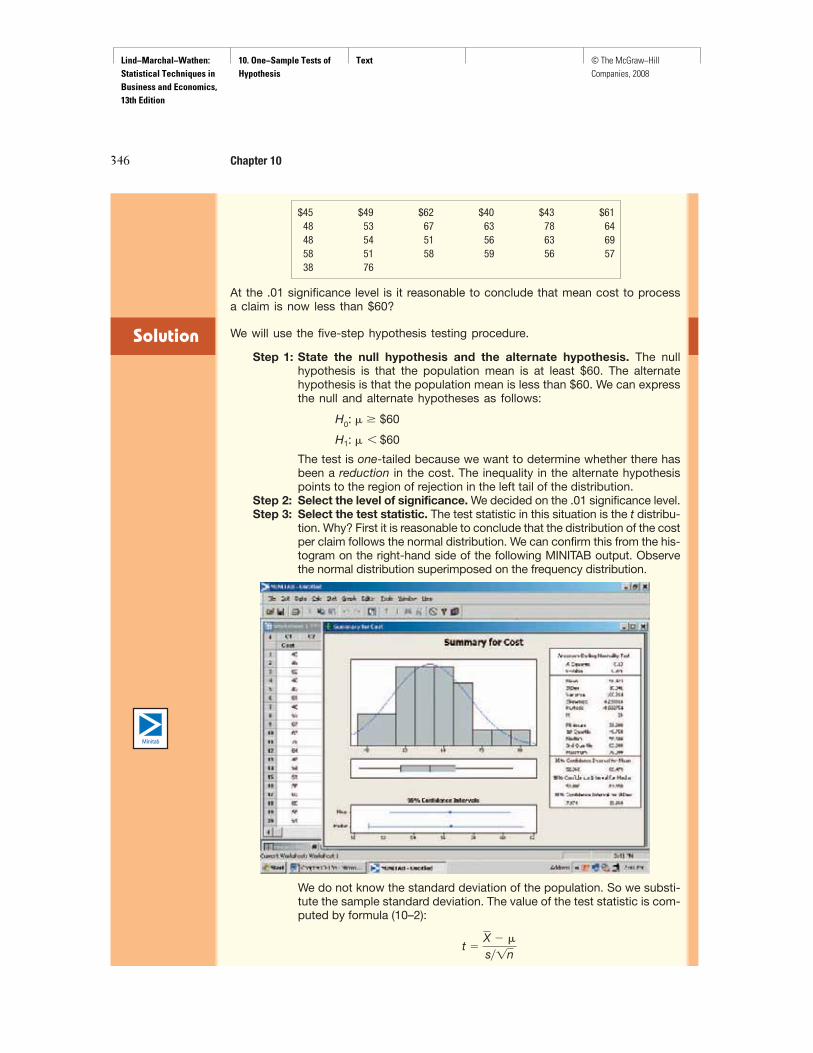
$45 $49 $62 $40 $43 $6148 53 67 63 78 6448 54 51 56 63 6958 51 58 59 56 5738 76
At the .01 significance level is it reasonable to conclude that mean cost to processa claim is now less than $60?
We will use the five-step hypothesis testing procedure.
Step 1: State the null hypothesis and the alternate hypothesis. The nullhypothesis is that the population mean is at least $60. The alternatehypothesis is that the population mean is less than $60. We can expressthe null and alternate hypotheses as follows:
The test is one-tailed because we want to determine whether there hasbeen a reduction in the cost. The inequality in the alternate hypothesispoints to the region of rejection in the left tail of the distribution.
Step 2: Select the level of significance. We decided on the .01 significance level.Step 3: Select the test statistic. The test statistic in this situation is the t distribu-
tion. Why? First it is reasonable to conclude that the distribution of the costper claim follows the normal distribution. We can confirm this from the his-togram on the right-hand side of the following MINITAB output. Observethe normal distribution superimposed on the frequency distribution.
H1: � 6 $60
H0: � $60
Solution
We do not know the standard deviation of the population. So we substi-tute the sample standard deviation. The value of the test statistic is com-puted by formula (10–2):
t �X �
s�1n
Lind−Marchal−Wathen: Statistical Techniques in Business and Economics, 13th Edition
10. One−Sample Tests of Hypothesis
Text © The McGraw−Hill Companies, 2008
One-Sample Tests of Hypothesis 347
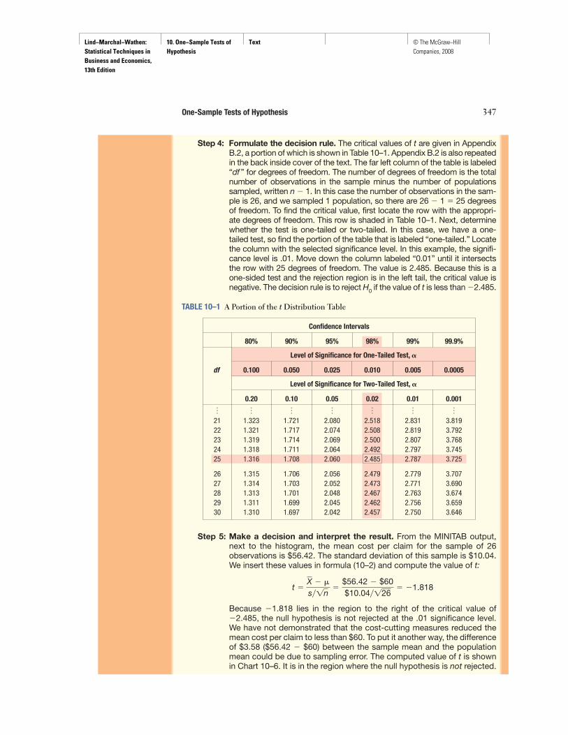
Step 4: Formulate the decision rule. The critical values of t are given in AppendixB.2, a portion of which is shown in Table 10–1. Appendix B.2 is also repeatedin the back inside cover of the text. The far left column of the table is labeled“df ” for degrees of freedom. The number of degrees of freedom is the totalnumber of observations in the sample minus the number of populationssampled, written n 1. In this case the number of observations in the sam-ple is 26, and we sampled 1 population, so there are 26 1 � 25 degreesof freedom. To find the critical value, first locate the row with the appropri-ate degrees of freedom. This row is shaded in Table 10–1. Next, determinewhether the test is one-tailed or two-tailed. In this case, we have a one-tailed test, so find the portion of the table that is labeled “one-tailed.” Locatethe column with the selected significance level. In this example, the signifi-cance level is .01. Move down the column labeled “0.01” until it intersectsthe row with 25 degrees of freedom. The value is 2.485. Because this is aone-sided test and the rejection region is in the left tail, the critical value isnegative. The decision rule is to reject H0 if the value of t is less than 2.485.
Confidence Intervals
80% 90% 95% 98% 99% 99.9%
Level of Significance for One-Tailed Test, �
df 0.100 0.050 0.025 0.010 0.005 0.0005
Level of Significance for Two-Tailed Test, �
0.20 0.10 0.05 0.02 0.01 0.001
o o o o o o o21 1.323 1.721 2.080 2.518 2.831 3.81922 1.321 1.717 2.074 2.508 2.819 3.79223 1.319 1.714 2.069 2.500 2.807 3.76824 1.318 1.711 2.064 2.492 2.797 3.74525 1.316 1.708 2.060 2.485 2.787 3.725
26 1.315 1.706 2.056 2.479 2.779 3.70727 1.314 1.703 2.052 2.473 2.771 3.69028 1.313 1.701 2.048 2.467 2.763 3.67429 1.311 1.699 2.045 2.462 2.756 3.65930 1.310 1.697 2.042 2.457 2.750 3.646
TABLE 10–1 A Portion of the t Distribution Table
Step 5: Make a decision and interpret the result. From the MINITAB output,next to the histogram, the mean cost per claim for the sample of 26observations is $56.42. The standard deviation of this sample is $10.04.We insert these values in formula (10–2) and compute the value of t:
Because 1.818 lies in the region to the right of the critical value ofthe null hypothesis is not rejected at the .01 significance level.
We have not demonstrated that the cost-cutting measures reduced themean cost per claim to less than $60. To put it another way, the differenceof $3.58 ($56.42 $60) between the sample mean and the populationmean could be due to sampling error. The computed value of t is shownin Chart 10–6. It is in the region where the null hypothesis is not rejected.
2.485,
t �X �
s�1n�
$56.42 $60$10.04�126
� 1.818
Lind−Marchal−Wathen: Statistical Techniques in Business and Economics, 13th Edition
10. One−Sample Tests of Hypothesis
Text © The McGraw−Hill Companies, 2008
In the previous example the mean and the standard deviation were computed usingMINITAB. The following example shows the details when the sample mean andsample standard deviation are calculated from sample data.
348 Chapter 10
0–1.818Computedvalue of t
Region of rejection
–2.485Criticalvalue
Scale of t
α = .01
H0: μ ≥ $60H1: μ < $60
df = 26 − 1 = 25
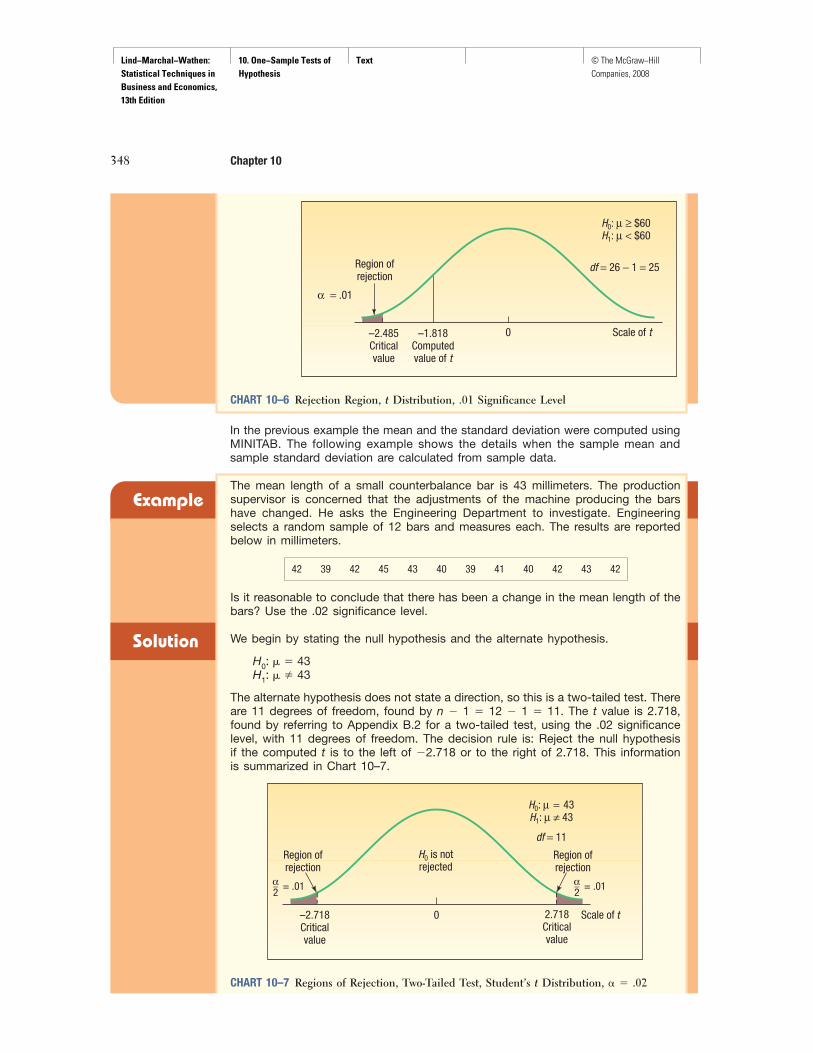
CHART 10–6 Rejection Region, t Distribution, .01 Significance Level
Example
Solution
The mean length of a small counterbalance bar is 43 millimeters. The productionsupervisor is concerned that the adjustments of the machine producing the barshave changed. He asks the Engineering Department to investigate. Engineeringselects a random sample of 12 bars and measures each. The results are reportedbelow in millimeters.
42 39 42 45 43 40 39 41 40 42 43 42
Is it reasonable to conclude that there has been a change in the mean length of thebars? Use the .02 significance level.
We begin by stating the null hypothesis and the alternate hypothesis.
The alternate hypothesis does not state a direction, so this is a two-tailed test. Thereare 11 degrees of freedom, found by n 1 � 12 1 � 11. The t value is 2.718,found by referring to Appendix B.2 for a two-tailed test, using the .02 significancelevel, with 11 degrees of freedom. The decision rule is: Reject the null hypothesisif the computed t is to the left of 2.718 or to the right of 2.718. This informationis summarized in Chart 10–7.
H1: � � 43H0: � � 43
CHART 10–7 Regions of Rejection, Two-Tailed Test, Student’s t Distribution, � � .02
0
Region of rejection
–2.718Criticalvalue
Scale of t
H0: μ = 43H1: μ ≠ 43
df = 11
H0 is notrejected
Region of rejection
2.718Criticalvalue
α_2
= .01 α_2
= .01

Lind−Marchal−Wathen: Statistical Techniques in Business and Economics, 13th Edition
10. One−Sample Tests of Hypothesis
Text © The McGraw−Hill Companies, 2008
One-Sample Tests of Hypothesis 349
We calculate the standard deviation of the sample using formula (3–11). Themean, , is 41.5 millimeters, and the standard deviation, s, is 1.784 millimeters. Thedetails are shown in Table 10–2.
X
TABLE 10–2 Calculations of the Sample Standard Deviation
X(mm) X � (X � )2
42 0.5 0.2539 2.5 6.2542 0.5 0.2545 3.5 12.2543 1.5 2.2540 1.5 2.2539 2.5 6.2541 0.5 0.2540 1.5 2.2542 0.5 0.2543 1.5 2.2542 0.5 0.25
498 0 35.00
s � B�(X X )2
n 1� B
3512 1
� 1.784
X �49812
� 41.5 mm
XX
Now we are ready to compute the value of t, using formula (10–2).
The null hypothesis that the population mean is 43 millimeters is rejectedbecause the computed t of 2.913 lies in the area to the left of 2.718. We acceptthe alternate hypothesis and conclude that the population mean is not 43 millime-ters. The machine is out of control and needs adjustment.
t �X �
s�1n�
41.5 43.01.784�112
� 2.913
Exercises9. Given the following hypothesis:
For a random sample of 10 observations, the sample mean was 12 and the sample stan-dard deviation 3. Using the .05 significance level:a. State the decision rule.b. Compute the value of the test statistic.c. What is your decision regarding the null hypothesis?
10. Given the following hypothesis:
For a random sample of 12 observations, the sample mean was 407 and the samplestandard deviation 6. Using the .01 significance level:a. State the decision rule.b. Compute the value of the test statistic.c. What is your decision regarding the null hypothesis?
H1: � � 400H0: � � 400
H1: � 7 10H0: � � 10
Self-Review 10–3 The mean life of a battery used in a digital clock is 305 days. The lives of the batteriesfollow the normal distribution. The battery was recently modified to last longer. A sampleof 20 of the modified batteries had a mean life of 311 days with a standard deviation of12 days. Did the modification increase the mean life of the battery?(a) State the null hypothesis and the alternate hypothesis.(b) Show the decision rule graphically. Use the .05 significance level.(c) Compute the value of t. What is your decision regarding the null hypothesis? Briefly
summarize your results.
Lind−Marchal−Wathen: Statistical Techniques in Business and Economics, 13th Edition
10. One−Sample Tests of Hypothesis
Text © The McGraw−Hill Companies, 2008
350 Chapter 10
11. The Rocky Mountain district sales manager of Rath Publishing, Inc., a college textbook pub-lishing company, claims that the sales representatives make an average of 40 sales calls perweek on professors. Several reps say that this estimate is too low. To investigate, a randomsample of 28 sales representatives reveals that the mean number of calls made last weekwas 42. The standard deviation of the sample is 2.1 calls. Using the .05 significance level,can we conclude that the mean number of calls per salesperson per week is more than 40?
12. The management of White Industries is considering a new method of assembling its golfcart. The present method requires 42.3 minutes, on the average, to assemble a cart. Themean assembly time for a random sample of 24 carts, using the new method, was 40.6minutes, and the standard deviation of the sample was 2.7 minutes. Using the .10 levelof significance, can we conclude that the assembly time using the new method is faster?
13. A spark plug manufacturer claimed that its plugs have a mean life in excess of 22,100 miles.Assume the life of the spark plugs follows the normal distribution. A fleet owner pur-chased a large number of sets. A sample of 18 sets revealed that the mean life was23,400 miles and the standard deviation was 1,500 miles. Is there enough evidence tosubstantiate the manufacturer’s claim at the .05 significance level?
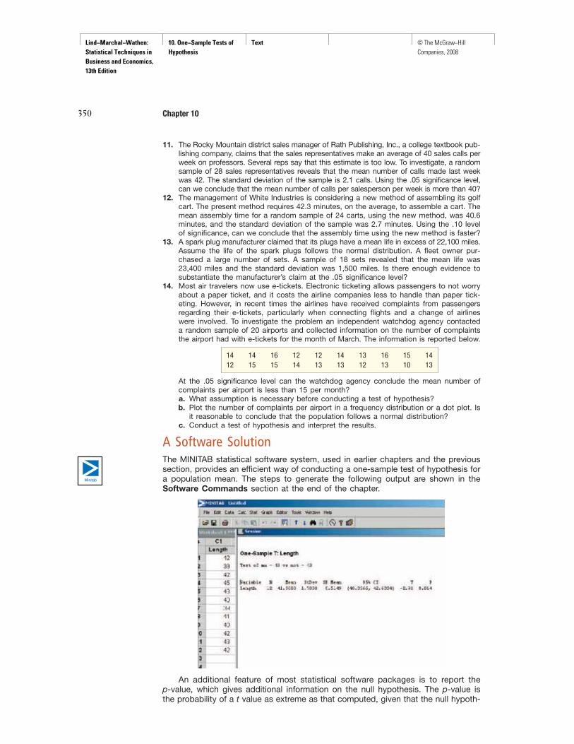
14. Most air travelers now use e-tickets. Electronic ticketing allows passengers to not worryabout a paper ticket, and it costs the airline companies less to handle than paper tick-eting. However, in recent times the airlines have received complaints from passengersregarding their e-tickets, particularly when connecting flights and a change of airlineswere involved. To investigate the problem an independent watchdog agency contacteda random sample of 20 airports and collected information on the number of complaintsthe airport had with e-tickets for the month of March. The information is reported below.
At the .05 significance level can the watchdog agency conclude the mean number ofcomplaints per airport is less than 15 per month?a. What assumption is necessary before conducting a test of hypothesis?b. Plot the number of complaints per airport in a frequency distribution or a dot plot. Is
it reasonable to conclude that the population follows a normal distribution?c. Conduct a test of hypothesis and interpret the results.
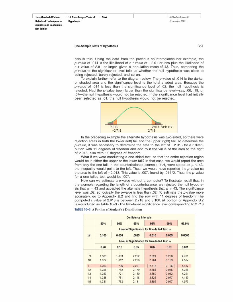
A Software SolutionThe MINITAB statistical software system, used in earlier chapters and the previoussection, provides an efficient way of conducting a one-sample test of hypothesis fora population mean. The steps to generate the following output are shown in the Software Commands section at the end of the chapter.
14 14 16 12 12 14 13 16 15 1412 15 15 14 13 13 12 13 10 13
An additional feature of most statistical software packages is to report thep-value, which gives additional information on the null hypothesis. The p-value isthe probability of a t value as extreme as that computed, given that the null hypoth-
Lind−Marchal−Wathen: Statistical Techniques in Business and Economics, 13th Edition
10. One−Sample Tests of Hypothesis
Text © The McGraw−Hill Companies, 2008
One-Sample Tests of Hypothesis 351
esis is true. Using the data from the previous counterbalance bar example, thep-value of .014 is the likelihood of a t value of 2.91 or less plus the likelihood ofa t value of 2.91 or larger, given a population mean of 43. Thus, comparing thep-value to the significance level tells us whether the null hypothesis was close tobeing rejected, barely rejected, and so on.
To explain further, refer to the diagram below. The p-value of .014 is the darkeror shaded area and the significance level is the total shaded area. Because thep-value of .014 is less than the significance level of .02, the null hypothesis isrejected. Had the p-value been larger than the significance level—say, .06, .19, or.57—the null hypothesis would not be rejected. If the significance level had initiallybeen selected as .01, the null hypothesis would not be rejected.
–2.913 2.913 Scale of t –2.718 2.718
TABLE 10–3 A Portion of Student’s t Distribution
Confidence Intervals
80% 90% 95% 98% 99% 99.9%
Level of Significance for One-Tailed Test, �
df 0.100 0.050 .0025 0.010 0.005 0.0005
Level of Significance for Two-Tailed Test, �
0.20 0.10 0.05 0.02 0.01 0.001
o o o o o o o9 1.383 1.833 2.262 2.821 3.250 4.781
10 1.372 1.812 2.228 2.764 3.169 4.587
11 1.363 1.796 2.201 2.718 3.106 4.43712 1.356 1.782 2.179 2.681 3.055 4.31813 1.350 1.771 2.160 2.650 3.012 4.22114 1.345 1.761 2.145 2.624 2.977 4.14015 1.341 1.753 2.131 2.602 2.947 4.073
In the preceding example the alternate hypothesis was two-sided, so there wererejection areas in both the lower (left) tail and the upper (right) tail. To determine thep-value, it was necessary to determine the area to the left of 2.913 for a t distri-bution with 11 degrees of freedom and add to it the value of the area to the rightof 2.913, also with 11 degrees of freedom.
What if we were conducting a one-sided test, so that the entire rejection regionwould be in either the upper or the lower tail? In that case, we would report the areafrom only the one tail. In the counterbalance example, if H1 were stated as � � 43,the inequality would point to the left. Thus, we would have reported the p-value asthe area to the left of 2.913. This value is .007, found by .014�2. Thus, the p-valuefor a one-tailed test would be .007.
How can we estimate a p-value without a computer? To illustrate, recall that, inthe example regarding the length of a counterbalance, we rejected the null hypothe-sis that � � 43 and accepted the alternate hypothesis that � � 43. The significancelevel was .02, so logically the p-value is less than .02. To estimate the p-value moreaccurately, go to Appendix B.2 and find the row with 11 degrees of freedom. Thecomputed t value of 2.913 is between 2.718 and 3.106. (A portion of Appendix B.2is reproduced as Table 10–3.) The two-tailed significance level corresponding to 2.718
Lind−Marchal−Wathen: Statistical Techniques in Business and Economics, 13th Edition
10. One−Sample Tests of Hypothesis
Text © The McGraw−Hill Companies, 2008
352 Chapter 10
Exercises15. Given the following hypothesis:
A random sample of five resulted in the following values: 18, 15, 12, 19, and 21. Usingthe .01 significance level, can we conclude the population mean is less than 20?a. State the decision rule.b. Compute the value of the test statistic.c. What is your decision regarding the null hypothesis?d. Estimate the p-value.
16. Given the following hypothesis:
A random sample of six resulted in the following values: 118, 105, 112, 119, 105, and111. Using the .05 significance level, can we conclude the mean is different from 100?a. State the decision rule.b. Compute the value of the test statistic.c. What is your decision regarding the null hypothesis?d. Estimate the p-value.
17. Experience raising New Jersey Red chickens revealed the mean weight of the chickensat five months is 4.35 pounds. The weights follow the normal distribution. In an effort toincrease their weight, a special additive is added to the chicken feed. The subsequentweights of a sample of five-month-old chickens were (in pounds):
At the .01 level, has the special additive increased the mean weight of the chickens?Estimate the p-value.
18. The liquid chlorine added to swimming pools to combat algae has a relatively short shelflife before it loses its effectiveness. Records indicate that the mean shelf life of a 5-gallonjug of chlorine is 2,160 hours (90 days). As an experiment, Holdlonger was added to thechlorine to find whether it would increase the shelf life. A sample of nine jugs of chlorinehad these shelf lives (in hours):
At the .025 level, has Holdlonger increased the shelf life of the chlorine? Estimate thep-value.
2,159 2,170 2,180 2,179 2,160 2,167 2,171 2,181 2,185
4.41 4.37 4.33 4.35 4.30 4.39 4.36 4.38 4.40 4.39
H1: � � 100H0: � � 100
H1: � 6 20H0: � 20
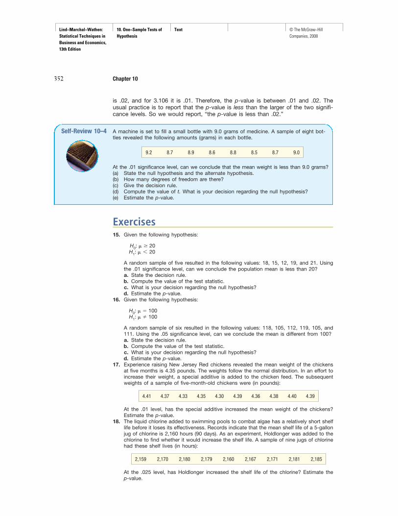
Self-Review 10–4 A machine is set to fill a small bottle with 9.0 grams of medicine. A sample of eight bot-tles revealed the following amounts (grams) in each bottle.
At the .01 significance level, can we conclude that the mean weight is less than 9.0 grams?(a) State the null hypothesis and the alternate hypothesis.(b) How many degrees of freedom are there?(c) Give the decision rule.(d) Compute the value of t. What is your decision regarding the null hypothesis?(e) Estimate the p-value.
9.2 8.7 8.9 8.6 8.8 8.5 8.7 9.0
is .02, and for 3.106 it is .01. Therefore, the p-value is between .01 and .02. Theusual practice is to report that the p-value is less than the larger of the two signifi-cance levels. So we would report, “the p-value is less than .02.”

Lind−Marchal−Wathen: Statistical Techniques in Business and Economics, 13th Edition
10. One−Sample Tests of Hypothesis
Text © The McGraw−Hill Companies, 2008
One-Sample Tests of Hypothesis 353
19. Wyoming fisheries contend that the mean number of cutthroat trout caught during a fullday of fly-fishing on the Snake, Buffalo, and other rivers and streams in the Jackson Holearea is 4.0. To make their yearly update, the fishery personnel asked a sample of flyfishermen to keep a count of the number caught during the day. The numbers were: 4,4, 3, 2, 6, 8, 7, 1, 9, 3, 1, and 6. At the .05 level, can we conclude that the mean num-ber caught is greater than 4.0? Estimate the p-value.
20. Hugger Polls contends that an agent conducts a mean of 53 in-depth home surveysevery week. A streamlined survey form has been introduced, and Hugger wants to eval-uate its effectiveness. The number of in-depth surveys conducted during a week by arandom sample of agents are:
At the .05 level of significance, can we conclude that the mean number of interviewsconducted by the agents is more than 53 per week? Estimate the p-value.
Tests Concerning ProportionsIn the previous chapter we discussed confidence intervals for proportions. We canalso conduct a test of hypothesis for a proportion. Recall that a proportion is the ratioof the number of successes to the number of observations. We let X refer to the num-ber of successes and n the number of observations, so the proportion of successesin a fixed number of trials is X�n. Thus, the formula for computing a sample propor-tion, p, is p � X�n. Consider the following potential hypothesis-testing situations.
• Historically, General Motors reports that 70 percent of leased vehicles arereturned with less than 36,000 miles. A recent sample of 200 vehicles returnedat the end of their lease showed 158 had less than 36,000 miles. Has the pro-portion increased?
• The American Association of Retired Persons (AARP) reports that 60 percent ofretired people under the age of 65 would return to work on a full-time basis if asuitable job were available. A sample of 500 retirees under 65 revealed 315 wouldreturn to work. Can we conclude that more than 60 percent would return to work?
• Able Moving and Storage, Inc., advises its clients for long-distance residentialmoves that their household goods will be delivered in 3 to 5 days from the timethey are picked up. Able’s records show it is successful 90 percent of the timewith this claim. A recent audit revealed it was successful 190 times out of 200.Can the company conclude its success rate has increased?
Some assumptions must be made and conditions met before testing a populationproportion. To test a hypothesis about a population proportion, a random sample ischosen from the population. It is assumed that the binomial assumptions discussedin Chapter 6 are met: (1) the sample data collected are the result of counts; (2)the outcome of an experiment is classified into one of two mutually exclusivecategories—a “success” or a “failure”; (3) the probability of a success is the samefor each trial; and (4) the trials are independent, meaning the outcome of one trialdoes not affect the outcome of any other trial. The test we will conduct shortly isappropriate when both n� and n(1 �) are at least 5. n is the sample size, and pis the population proportion. It takes advantage of the fact that a binomial distrib-ution can be approximated by the normal distribution.
53 57 50 55 58 54 60 52 59 62 60 60 51 59 56
n� and n (1 �) mustbe at least 5.
ExampleSuppose prior elections in a certain state indicated it is necessary for a candidatefor governor to receive at least 80 percent of the vote in the northern section of thestate to be elected. The incumbent governor is interested in assessing his chancesof returning to office and plans to conduct a survey of 2,000 registered voters inthe northern section of the state.
Using the hypothesis-testing procedure, assess the governor’s chances ofreelection.
Lind−Marchal−Wathen: Statistical Techniques in Business and Economics, 13th Edition
10. One−Sample Tests of Hypothesis
Text © The McGraw−Hill Companies, 2008
354 Chapter 10
Solution
Finding the criticalvalue
This situation regarding the governor’s reelection meets the binomial conditions.
• There are only two possible outcomes. That is, a sampled voter will either voteor not vote for the governor.
• The probability of a success is the same for each trial. In this case the likeli-hood a particular sampled voter will support reelection is .80.
• The trials are independent. This means, for example, the likelihood the 23rd votersampled will support reelection is not affected by what the 24th or 52nd voter does.
• The sample data is the result of counts. We are going to count the number ofvoters who support reelection in the sample of 2,000.
We can use the normal approximation to the binomial distribution, discussed inChapter 7, because both n� and n(1 �) exceed 5. In this case, n � 2,000 and� � .80 (� is the proportion of the vote in the northern part of the state, or 80 per-cent, needed to be elected). Thus, n� � 2,000(.80) � 1,600 and n(1 �) � 2,000(1 .80) � 400. Both 1,600 and 400 are greater than 5.
Step 1: State the null hypothesis and the alternate hypothesis. The nullhypothesis, H0, is that the population proportion is .80 or larger. Thealternate hypothesis, H1, is that the proportion is less than .80. From apractical standpoint, the incumbent governor is concerned only whenthe proportion is less than .80. If it is equal to or greater than .80, hewill have no problem; that is, the sample data would indicate he willprobably be reelected. These hypotheses are written symbolically as:
H1 states a direction. Thus, as noted previously, the test is one-tailed withthe inequality sign pointing to the tail of the distribution containing theregion of rejection.
Step 2: Select the level of significance. The level of significance is .05. This isthe likelihood that a true hypothesis will be rejected.
Step 3: Select the test statistic. z is the appropriate statistic, found by:
H1: � 6 .80H0: � .80
�
TEST OF HYPOTHESIS, ONE PROPORTION [10–3]z �
p �
A�(1 �)
n
where:� is the population proportion.p is the sample proportion.n is the sample size.
Step 4: Formulate the decision rule. The critical value or values of z form the di-viding point or points between the regions where H0 is rejected and whereit is not rejected. Since the alternate hypothesis states a direction, this isa one-tailed test. The sign of the inequality points to the left, so only theleft side of the curve is used. (See Chart 10–8.) The significance level wasgiven as .05 in step 2. This probability is in the left tail and determines theregion of rejection. The area between zero and the critical value is .4500,found by .5000 .0500. Referring to Appendix B.1 and searching for.4500, we find the critical value of z is 1.65. The decision rule is, therefore:Reject the null hypothesis and accept the alternate hypothesis if the com-puted value of z falls to the left of 1.65; otherwise do not reject H0.
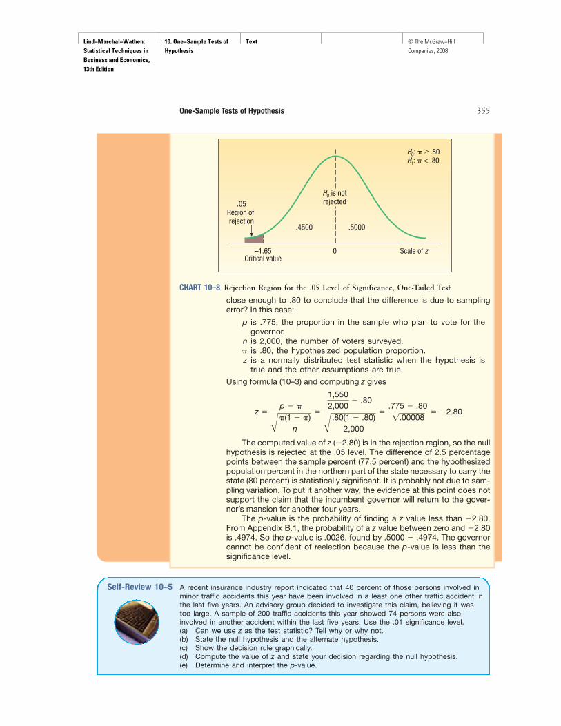
Step 5: Make a decision and interpret the result. Select a sample and make adecision about H0. A sample survey of 2,000 potential voters in the north-ern part of the state revealed that 1,550 planned to vote for the incum-bent governor. Is the sample proportion of .775 (found by 1,550�2,000)
Select a sample andmake a decisionregarding .H0
Lind−Marchal−Wathen: Statistical Techniques in Business and Economics, 13th Edition
10. One−Sample Tests of Hypothesis
Text © The McGraw−Hill Companies, 2008
One-Sample Tests of Hypothesis 355
.4500 .5000
H0: � ≥ .80H1: � < .80
0–1.65Critical value
Scale of z
.05Region of rejection
H0 is notrejected
CHART 10–8 Rejection Region for the .05 Level of Significance, One-Tailed Test
close enough to .80 to conclude that the difference is due to samplingerror? In this case:
p is .775, the proportion in the sample who plan to vote for thegovernor.
n is 2,000, the number of voters surveyed.� is .80, the hypothesized population proportion.z is a normally distributed test statistic when the hypothesis is
true and the other assumptions are true.
Using formula (10–3) and computing z gives
The computed value of z (2.80) is in the rejection region, so the nullhypothesis is rejected at the .05 level. The difference of 2.5 percentagepoints between the sample percent (77.5 percent) and the hypothesizedpopulation percent in the northern part of the state necessary to carry thestate (80 percent) is statistically significant. It is probably not due to sam-pling variation. To put it another way, the evidence at this point does notsupport the claim that the incumbent governor will return to the gover-nor’s mansion for another four years.
The p-value is the probability of finding a z value less than 2.80.From Appendix B.1, the probability of a z value between zero and 2.80is .4974. So the p-value is .0026, found by .5000 .4974. The governorcannot be confident of reelection because the p-value is less than thesignificance level.
z �p �
A�(1 �)
n
�
1,5502,000
.80
A.80(1 .80)
2,000
�.775 .801.00008
� 2.80
Self-Review 10–5 A recent insurance industry report indicated that 40 percent of those persons involved inminor traffic accidents this year have been involved in a least one other traffic accident inthe last five years. An advisory group decided to investigate this claim, believing it wastoo large. A sample of 200 traffic accidents this year showed 74 persons were alsoinvolved in another accident within the last five years. Use the .01 significance level.(a) Can we use z as the test statistic? Tell why or why not.(b) State the null hypothesis and the alternate hypothesis.(c) Show the decision rule graphically.(d) Compute the value of z and state your decision regarding the null hypothesis.(e) Determine and interpret the p-value.

Lind−Marchal−Wathen: Statistical Techniques in Business and Economics, 13th Edition
10. One−Sample Tests of Hypothesis
Text © The McGraw−Hill Companies, 2008
356 Chapter 10
Exercises21. The following hypotheses are given.
A sample of 100 observations revealed that p � .75. At the .05 significance level, canthe null hypothesis be rejected?a. State the decision rule.b. Compute the value of the test statistic.c. What is your decision regarding the null hypothesis?
22. The following hypotheses are given.
A sample of 120 observations revealed that p � .30. At the .05 significance level, canthe null hypothesis be rejected?a. State the decision rule.b. Compute the value of the test statistic.c. What is your decision regarding the null hypothesis?
Note: It is recommended that you use the five-step hypothesis-testing procedure in solvingthe following problems.
23. The National Safety Council reported that 52 percent of American turnpike drivers aremen. A sample of 300 cars traveling southbound on the New Jersey Turnpike yesterdayrevealed that 170 were driven by men. At the .01 significance level, can we conclude thata larger proportion of men were driving on the New Jersey Turnpike than the nationalstatistics indicate?
24. A recent article in USA Today reported that a job awaits only one in three new collegegraduates. The major reasons given were an overabundance of college graduates and aweak economy. A survey of 200 recent graduates from your school revealed that 80 stu-dents had jobs. At the .02 significance level, can we conclude that a larger proportion ofstudents at your school have jobs?
25. Chicken Delight claims that 90 percent of its orders are delivered within 10 minutes ofthe time the order is placed. A sample of 100 orders revealed that 82 were deliveredwithin the promised time. At the .10 significance level, can we conclude that less than90 percent of the orders are delivered in less than 10 minutes?
26. Research at the University of Toledo indicates that 50 percent of students change theirmajor area of study after their first year in a program. A random sample of 100 studentsin the College of Business revealed that 48 had changed their major area of study aftertheir first year of the program. Has there been a significant decrease in the proportion ofstudents who change their major after the first year in this program? Test at the .05 levelof significance.
Type II ErrorRecall that the level of significance, identified by the symbol �, is the probabilitythat the null hypothesis is rejected when it is true. This is called a Type I error. Themost common levels of significance are .05 and .01 and are set by the researcherat the outset of the test.
In a hypothesis-testing situation there is also the possibility that a null hypothesisis not rejected when it is actually false. That is, we accept a false null hypothesis. Thisis called a Type II error. The probability of a Type II error is identified by the Greek let-ter beta (�). The following examples illustrate the details of determining the value of �.
H1: � � .40H0: � � .40
H1: � 7 .70H0: � � .70
ExampleA manufacturer purchases steel bars to make cotter pins. Past experience indicatesthat the mean tensile strength of all incoming shipments is 10,000 psi and that thestandard deviation, �, is 400 psi.
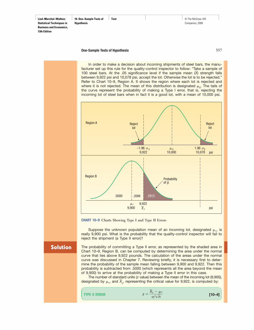
Lind−Marchal−Wathen: Statistical Techniques in Business and Economics, 13th Edition
10. One−Sample Tests of Hypothesis
Text © The McGraw−Hill Companies, 2008
One-Sample Tests of Hypothesis 357
Solution
CHART 10–9 Charts Showing Type I and Type II Errors
09,922
Rejectlot
Rejectlot
10,07810,000–1.96 � x– 1.96 �x–
Region A
Probabilityof �
psi
psi
�
9,9009,922
.2912.2088.5000
�1
X c
Region B
In order to make a decision about incoming shipments of steel bars, the manu-facturer set up this rule for the quality-control inspector to follow: “Take a sample of100 steel bars. At the .05 significance level if the sample mean strength fallsbetween 9,922 psi and 10,078 psi, accept the lot. Otherwise the lot is to be rejected.”Refer to Chart 10–9, Region A. It shows the region where each lot is rejected andwhere it is not rejected. The mean of this distribution is designated �0. The tails ofthe curve represent the probability of making a Type I error, that is, rejecting theincoming lot of steel bars when in fact it is a good lot, with a mean of 10,000 psi.
(X)
Suppose the unknown population mean of an incoming lot, designated �1, isreally 9,900 psi. What is the probability that the quality-control inspector will fail toreject the shipment (a Type II error)?
The probability of committing a Type II error, as represented by the shaded area inChart 10–9, Region B, can be computed by determining the area under the normalcurve that lies above 9,922 pounds. The calculation of the areas under the normalcurve was discussed in Chapter 7. Reviewing briefly, it is necessary first to deter-mine the probability of the sample mean falling between 9,900 and 9,922. Then thisprobability is subtracted from .5000 (which represents all the area beyond the meanof 9,900) to arrive at the probability of making a Type II error in this case.
The number of standard units (z value) between the mean of the incoming lot (9,900),designated by �1, and , representing the critical value for 9,922, is computed by:
TYPE II ERROR [10–4] z �Xc �1
��1n
Xc

Lind−Marchal−Wathen: Statistical Techniques in Business and Economics, 13th Edition
10. One−Sample Tests of Hypothesis
Text © The McGraw−Hill Companies, 2008
358 Chapter 10
With n � 100 and � � 400, the value of z is 0.55:
The area under the curve between 9,900 and 9,922 (a z value of 0.55) is .2088. Thearea under the curve beyond 9,922 pounds is .5000 .2088, or .2912; this is theprobability of making a Type II error—that is, accepting an incoming lot of steel barswhen the population mean is 9,900 psi.
Another illustration, in Chart 10–10, Region C, depicts the probability of accept-ing a lot when the population mean is 10,120. To find the probability:
The probability that z is less than 1.05 is .1469, found by .5000 .3531. There-fore, �, or the probability of a Type II error, is .1469.
z �Xc �1
��1n�
10,078 10,120400�1100
� 1.05
z �Xc �1
��1n�
9,922 9,900400�1100
�2240
� 0.55
0
9,922
Rejectionregion
Rejectionregion
10,07810,000–1.96 �– 1.96 ��
�
xx –
2� .025�
2� .025�
10,12010,078
1
Probabilityof makinga Type II
errorProbability
of not makinga Type II
error
Probabilityof not making
a Type IIerror
� 1�
Xc
Region A
Region C
psi
psi
CHART 10–10 Type I and Type II Errors (Another Example)
Using the methods illustrated by Charts 10–9 Region B and 10-10 Region C,the probability of accepting a hypothesis as true when it is actually false can bedetermined for any value of �1.
Type II error probabilities are shown in the center column of Table 10–4 forselected values of �, given in the left column. The right column gives the probabil-ity of not making a Type II error, which is also known as the power of a test.
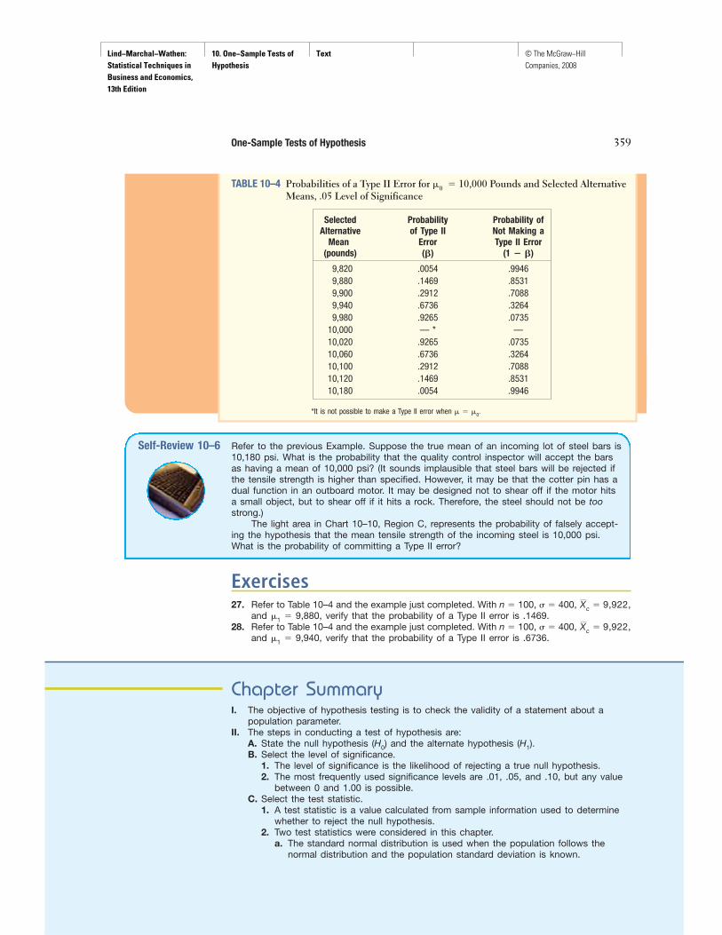
Lind−Marchal−Wathen: Statistical Techniques in Business and Economics, 13th Edition
10. One−Sample Tests of Hypothesis
Text © The McGraw−Hill Companies, 2008
Chapter SummaryI. The objective of hypothesis testing is to check the validity of a statement about a
population parameter.II. The steps in conducting a test of hypothesis are:
A. State the null hypothesis (H0) and the alternate hypothesis (H1).B. Select the level of significance.
1. The level of significance is the likelihood of rejecting a true null hypothesis.2. The most frequently used significance levels are .01, .05, and .10, but any value
between 0 and 1.00 is possible.C. Select the test statistic.
1. A test statistic is a value calculated from sample information used to determinewhether to reject the null hypothesis.
2. Two test statistics were considered in this chapter.a. The standard normal distribution is used when the population follows the
normal distribution and the population standard deviation is known.
One-Sample Tests of Hypothesis 359
Exercises27. Refer to Table 10–4 and the example just completed. With n � 100, � � 400,
and �1 � 9,880, verify that the probability of a Type II error is .1469.28. Refer to Table 10–4 and the example just completed. With n � 100, � � 400,
and �1 � 9,940, verify that the probability of a Type II error is .6736.Xc � 9,922,
Xc � 9,922,
TABLE 10–4 Probabilities of a Type II Error for �0 � 10,000 Pounds and Selected AlternativeMeans, .05 Level of Significance
Selected Probability Probability ofAlternative of Type II Not Making a
Mean Error Type II Error(pounds) (�) (1 � �)
9,820 .0054 .99469,880 .1469 .85319,900 .2912 .70889,940 .6736 .32649,980 .9265 .0735
10,000 — * —10,020 .9265 .073510,060 .6736 .326410,100 .2912 .708810,120 .1469 .853110,180 .0054 .9946
*It is not possible to make a Type II error when � � �0.
Self-Review 10–6 Refer to the previous Example. Suppose the true mean of an incoming lot of steel bars is10,180 psi. What is the probability that the quality control inspector will accept the barsas having a mean of 10,000 psi? (It sounds implausible that steel bars will be rejected ifthe tensile strength is higher than specified. However, it may be that the cotter pin has adual function in an outboard motor. It may be designed not to shear off if the motor hitsa small object, but to shear off if it hits a rock. Therefore, the steel should not be toostrong.)
The light area in Chart 10–10, Region C, represents the probability of falsely accept-ing the hypothesis that the mean tensile strength of the incoming steel is 10,000 psi.What is the probability of committing a Type II error?

Lind−Marchal−Wathen: Statistical Techniques in Business and Economics, 13th Edition
10. One−Sample Tests of Hypothesis
Text © The McGraw−Hill Companies, 2008
360 Chapter 10
b. The t distribution is used when the population follows the normal distributionand the population standard deviation is unknown.
D. State the decision rule.1. The decision rule indicates the condition or conditions when the null hypothesis
is rejected.2. In a two-tailed test, the rejection region is evenly split between the upper and
lower tails.3. In a one-tailed test, all of the rejection region is in either the upper or the
lower tail.E. Select a sample, compute the value of the test statistic, make a decision regarding
the null hypothesis, and interpret the results.III. A p-value is the probability that the value of the test statistic is as extreme as the value
computed, when the null hypothesis is true.IV. When testing a hypothesis about a population mean:
A. If the population standard deviation, �, is known, the test statistic is the standardnormal distribution and is determined from:
[10–1]
B. If the population standard deviation is not known, s is substituted for �. The teststatistic is the t distribution, and its value is determined from:
[10–2]
The major characteristics of the t distribution are:1. It is a continuous distribution.2. It is mound-shaped and symmetrical.3. It is flatter, or more spread out, than the standard normal distribution.4. There is a family of t distributions, depending on the number of degrees of freedom.
V. When testing about a population proportion:A. The binomial conditions must be met.B. Both n� and n(1 �) must be at least 5.C. The test statistic is
[10–3]
VI. There are two types of errors that can occur in a test of hypothesis.A. A Type I error occurs when a true null hypothesis is rejected.
1. The probability of making a Type I error is equal to the level of significance.2. This probability is designated by the Greek letter �.
B. A Type II error occurs when a false null hypothesis is not rejected.1. The probability of making a Type II error is designated by the Greek letter �.2. The likelihood of a Type II error is found by
[10–4]
Pronunciation Key
z �Xc �1
��1n
z �p �
A�(1 �)
n
t �X �
s�1n
z �X �
��1n
SYMBOL MEANING PRONUNCIATION
H0 Null hypothesis H sub zero
H1 Alternate hypothesis H sub one
�/2 Two-tailed significance level Alpha over 2
c Limit of the sample mean X bar sub c
�0 Assumed population mean mu sub zero
X

Lind−Marchal−Wathen: Statistical Techniques in Business and Economics, 13th Edition
10. One−Sample Tests of Hypothesis
Text © The McGraw−Hill Companies, 2008
One-Sample Tests of Hypothesis 361One-Sample Tests of Hypothesis 361
45.6 47.7 47.6 46.3 46.2 47.4 49.2 55.8 47.5 48.5
Chapter Exercises29. According to the local union president, the mean gross income of plumbers in the Salt Lake
City area follows the normal probability distribution with a mean of $45,000 and a standarddeviation of $3,000. A recent investigative reporter for KYAK TV found, for a sample of 120plumbers, the mean gross income was $45,500. At the .10 significance level, is it reason-able to conclude that the mean income is not equal to $45,000? Determine the p-value.
30. Rutter Nursery Company packages its pine bark mulch in 50-pound bags. From a long his-tory, the production department reports that the distribution of the bag weights follows thenormal distribution and the standard deviation of this process is 3 pounds per bag. Atthe end of each day, Jeff Rutter, the production manager, weighs 10 bags and computesthe mean weight of the sample. Below are the weights of 10 bags from today’s production.
a. Can Mr. Rutter conclude that the mean weight of the bags is less than 50 pounds?Use the .01 significance level.
b. In a brief report, tell why Mr. Rutter can use the z distribution as the test statistic.c. Compute the p-value.
31. A new weight-watching company, Weight Reducers International, advertises that thosewho join will lose, on the average, 10 pounds the first two weeks with a standard deviationof 2.8 pounds. A random sample of 50 people who joined the new weight reduction pro-gram revealed the mean loss to be 9 pounds. At the .05 level of significance, can weconclude that those joining Weight Reducers on average will lose less than 10 pounds?Determine the p-value.
32. Dole Pineapple, Inc., is concerned that the 16-ounce can of sliced pineapple is beingoverfilled. Assume the standard deviation of the process is .03 ounces. The quality-control department took a random sample of 50 cans and found that the arithmetic meanweight was 16.05 ounces. At the 5 percent level of significance, can we conclude thatthe mean weight is greater than 16 ounces? Determine the p-value.
33. According to a recent survey, Americans get a mean of 7 hours of sleep per night. A ran-dom sample of 50 students at West Virginia University revealed the mean number ofhours slept last night was 6 hours and 48 minutes (6.8 hours). The standard deviation ofthe sample was 0.9 hours. Is it reasonable to conclude that students at West Virginiasleep less than the typical American? Compute the p-value.
34. A statewide real estate sales agency, Farm Associates, specializes in selling farm propertyin the state of Nebraska. Its records indicate that the mean selling time of farm propertyis 90 days. Because of recent drought conditions, the agency believes that the meanselling time is now greater than 90 days. A statewide survey of 100 farms sold recentlyrevealed that the mean selling time was 94 days, with a standard deviation of 22 days.At the .10 significance level, has there been an increase in selling time?
35. NBC TV news, in a segment on the price of gasoline, reported last evening that the meanprice nationwide is $2.50 per gallon for self-serve regular unleaded. A random sample of35 stations in the Milwaukee, Wisconsin, area revealed that the mean price was $2.52per gallon and that the standard deviation was $0.05 per gallon. At the .05 significancelevel, can we conclude that the price of gasoline is higher in the Milwaukee area? Deter-mine the p-value.
36. A recent article in Vitality magazine reported that the mean amount of leisure time perweek for American men is 40.0 hours. You believe this figure is too large and decide toconduct your own test. In a random sample of 60 men, you find that the mean is37.8 hours of leisure per week and that the standard deviation of the sample is12.2 hours. Can you conclude that the information in the article is untrue? Use the .05 sig-nificance level. Determine the p-value and explain its meaning.
37. In recent years the interest rate on home mortgages has declined to less than 6.0 per-cent. However, according to a study by the Federal Reserve Board the rate charged oncredit card debt is more than 14 percent. Listed below is the interest rate charged on asample of 10 credit cards.
14.6 16.7 17.4 17.0 17.8 15.4 13.1 15.8 14.3 14.5
Lind−Marchal−Wathen: Statistical Techniques in Business and Economics, 13th Edition
10. One−Sample Tests of Hypothesis
Text © The McGraw−Hill Companies, 2008
362 Chapter 10
4.8 5.3 6.5 4.8 6.1 5.8 6.2 5.6
3.1 3.3 3.5 2.6 2.6 4.3 4.4 3.8 3.1 4.1 3.1 3.2
25 27 25 26 25 28 28 27 24 26 25 29 25 27 24
0 4 3 4 9 4 5 9 1 6 7 10
2.98 2.40 2.70 2.25 3.23 3.17 2.93 3.18 2.802.38 3.75 3.20 3.27 2.52 2.58 4.45 2.45
Is it reasonable to conclude the mean rate charged is greater than 14 percent? Use the.01 significance level.
38. A recent article in The Wall Street Journal reported that the 30-year mortgage rate is nowless than 6 percent. A sample of eight small banks in the Midwest revealed the follow-ing 30-year rates (in percent):
At the .01 significance level, can we conclude that the 30-year mortgage rate for smallbanks is less than 6 percent? Estimate the p-value.
39. According to the Coffee Research Organization (http://www.coffeeresearch.org) the typi-cal American coffee drinker consumes an average of 3.1 cups per day. A sample of 12senior citizens revealed they consumed the following amounts of coffee, reported in cups,yesterday.
At the .05 significance level does this sample data suggest there is a difference betweenthe national average and the sample mean from senior citizens?
40. The postanesthesia care area (recovery room) at St. Luke’s Hospital in Maumee, Ohio,was recently enlarged. The hope was that with the enlargement the mean number ofpatients per day would be more than 25. A random sample of 15 days revealed thefollowing numbers of patients.
At the .01 significance level, can we conclude that the mean number of patients per dayis more than 25? Estimate the p-value and interpret it.
41. eGolf.com receives an average of 6.5 returns per day from online shoppers. For a sam-ple of 12 days, it received the following number of returns.
At the .01 significance level, can we conclude the mean number of returns is lessthan 6.5?
42. During recent seasons, Major League Baseball has been criticized for the length of thegames. A report indicated that the average game lasts 3 hours and 30 minutes. A sam-ple of 17 games revealed the following times to completion. (Note that the minutes havebeen changed to fractions of hours, so that a game that lasted 2 hours and 24 minutesis reported at 2.40 hours.)
Can we conclude that the mean time for a game is less than 3.50 hours? Use the .05significance level.
43. Watch Corporation of Switzerland claims that its watches on average will neither gain norlose time during a week. A sample of 18 watches provided the following gains orlosses in seconds per week.()
(�)
Is it reasonable to conclude that the mean gain or loss in time for the watches is 0? Usethe .05 significance level. Estimate the p-value.
44. Listed below is the rate of return for one year (reported in percent) for a sample of 12mutual funds that are classified as taxable money market funds.
0.38 0.20 0.38 0.32 �0.32 0.23 �0.30 �0.25 0.100.37 0.61 0.48 0.47 0.64 0.04 0.20 0.68 �0.05
4.63 4.15 4.76 4.70 4.65 4.52 4.70 5.06 4.42 4.51 4.24 4.52

Lind−Marchal−Wathen: Statistical Techniques in Business and Economics, 13th Edition
10. One−Sample Tests of Hypothesis
Text © The McGraw−Hill Companies, 2008
One-Sample Tests of Hypothesis 363
120 108 120 114 118 91 118 92 104 104112 97 118 108 117
$321 $286 $290 $330 $310 $250 $270 $280 $299 $265 $291 $275 $281
Is it reasonable to conclude that the mean number of customers using the self-checkoutsystem is more than 100 per day? Use the .05 significance level.
46. In the year 2006 the mean fare to fly from Charlotte, North Carolina, to Seattle, Wash-ington, on a discount ticket was $267. A random sample of round-trip discount fares onthis route last month gives:
At the .01 significance level can we conclude that the mean fare has increased? What isthe p-value?
47. The publisher of Celebrity Living claims that the mean sales for personality magazinesthat feature people such as Angelina Jolie or Paris Hilton are 1.5 million copies per week.A sample of 10 comparable titles shows a mean weekly sales last week of 1.3 millioncopies with a standard deviation of 0.9 million copies. Does this data contradict the pub-lisher’s claim? Use the 0.01 significance level.
48. A United Nations report shows the mean family income for Mexican migrants to theUnited States is $27,000 per year. A FLOC (Farm Labor Organizing Committee) evalua-tion of 25 Mexican family units reveals a mean to be $30,000 with a sample standarddeviation of $10,000. Does this information disagree with the United Nations report?Apply the 0.01 significance level.
49. Traditionally, two percent of the citizens of the United States live in a foreign countrybecause they are disenchanted with U.S. politics or social attitudes. In order to test ifthis proportion has increased since the September 11, 2001, terror attacks, U.S. con-sulates contacted a random sample of 400 of these expatriates. The sample yields 12people who report they are living overseas because of political or social attitudes. Canyou conclude this data shows the proportion of politically motivated expatriates hasincreased? Use the 0.05 significance level.
50. According to a study by the American Pet Food Dealers Association, 63 percent of U.S.households own pets. A report is being prepared for an editorial in the San FranciscoChronicle. As a part of the editorial a random sample of 300 households showed 210own pets. Does this data disagree with the Pet Food Dealers Association data? Use a.05 level of significance.
51. Tina Dennis is the comptroller for Meek Industries. She believes that the current cash-flow problem at Meek is due to the slow collection of accounts receivable. She believesthat more than 60 percent of the accounts are in arrears more than three months. A ran-dom sample of 200 accounts showed that 140 were more than three months old. At the.01 significance level, can she conclude that more than 60 percent of the accounts arein arrears for more than three months?
52. The policy of the Suburban Transit Authority is to add a bus route if more than 55 per-cent of the potential commuters indicate they would use the particular route. A sampleof 70 commuters revealed that 42 would use a proposed route from Bowman Park tothe downtown area. Does the Bowman-to-downtown route meet the STA criterion? Usethe .05 significance level.
53. Past experience at the Crowder Travel Agency indicated that 44 percent of those personswho wanted the agency to plan a vacation for them wanted to go to Europe. During themost recent busy season, a sampling of 1,000 plans was selected at random from thefiles. It was found that 480 persons wanted to go to Europe on vacation. Has there beena significant shift upward in the percentage of persons who want to go to Europe? Testat the .05 significance level.
Using the .05 significance level is it reasonable to conclude that the mean rate of returnis more than 4.50 percent?
45. Many grocery stores and large retailers such as Wal-Mart and Kmart have installed self-checkout systems so shoppers can scan their own items and cash out themselves. Howdo customers like this service and how often do they use it? Listed below is the num-ber of customers using the service for a sample of 15 days at the Wal-Mart on Highway544 in Surfside, South Carolina.
Lind−Marchal−Wathen: Statistical Techniques in Business and Economics, 13th Edition
10. One−Sample Tests of Hypothesis
Text © The McGraw−Hill Companies, 2008
364 Chapter 10
54. From past experience a television manufacturer found that 10 percent or less of its setsneeded any type of repair in the first two years of operation. In a sample of 50 sets man-ufactured two years ago, 9 needed repair. At the .05 significance level, has the percentof sets needing repair increased? Determine the p-value.
55. An urban planner claims that, nationally, 20 percent of all families renting condominiumsmove during a given year. A random sample of 200 families renting condominiums in theDallas Metroplex revealed that 56 had moved during the past year. At the .01 significancelevel, does this evidence suggest that a larger proportion of condominium owners movedin the Dallas area? Determine the p-value.
56. The cost of weddings in the United States has skyrocketed in recent years. As a resultmany couples are opting to have their weddings in the Caribbean. A Caribbean vacationresort recently advertised in Bride Magazine that the cost of a Caribbean wedding wasless than $10,000. Listed below is a total cost in $000 for a sample of 8 Caribbeanweddings.
9.7 9.4 11.7 9.0 9.1 10.5 9.1 9.8
At the .05 significance level is it reasonable to conclude the mean wedding cost is lessthan $10,000 as advertised?
57. The U.S. president’s call for designing and building a missile defense system that ignoresrestrictions of the Anti-Ballistic Missile Defense System treaty (ABM) is supported by 483of the respondents in a nationwide poll of 1,002 adults. Is it reasonable to conclude thatthe nation is evenly divided on the issue? Use the .05 significance level.
58. One of the major U.S. automakers wishes to review its warranty. The warranty covers theengine, transmission, and drivetrain of all new cars for up to two years or 24,000 miles,whichever comes first. The manufacturer’s quality-assurance department believes that themean number of miles driven by owners is more than 24,000. A sample of 35 cars revealedthat the mean number of miles was 24,421, with a standard deviation of 1,944 miles.a. Conduct the following hypothesis test. Use the .05 significance level.
b. What is the largest value for the sample mean for which H0 is not rejected?c. Suppose the population mean shifts to 25,000 miles. What is the probability this
change will not be detected?59. A cola-dispensing machine is set to dispense 9.00 ounces of cola per cup, with a stan-
dard deviation of 1.00 ounces. The manufacturer of the machine would like to set thecontrol limit in such a way that, for samples of 36, 5 percent of the sample means willbe greater than the upper control limit, and 5 percent of the sample means will be lessthan the lower control limit.a. At what value should the control limit be set?b. What is the probability that if the population mean shifts to 8.9, this change will not
be detected?c. What is the probability that if the population mean shifts to 9.3, this change will not
be detected?60. The owners of the Franklin Park Mall wished to study customer shopping habits. From
earlier studies the owners were under the impression that a typical shopper spends 0.75hours at the mall, with a standard deviation of 0.10 hours. Recently the mall ownersadded some specialty restaurants designed to keep shoppers in the mall longer. The con-sulting firm, Brunner and Swanson Marketing Enterprises, was hired to evaluate theeffects of the restaurants. A sample of 45 shoppers by Brunner and Swanson revealedthat the mean time spent in the mall had increased to 0.80 hours.a. Develop a test of hypothesis to determine if the mean time spent in the mall is more
than 0.75 hours. Use the .05 significance level.b. Suppose the mean shopping time actually increased from 0.75 hours to 0.77 hours.
What is the probability this increase would not be detected?c. When Brunner and Swanson reported the information in part (b) to the mall own-
ers, the owners were upset with the statement that a survey could not detect achange from 0.75 to 0.77 hours of shopping time. How could this probability bereduced?
H1: � 7 24,000H0: � � 24,000

Lind−Marchal−Wathen: Statistical Techniques in Business and Economics, 13th Edition
10. One−Sample Tests of Hypothesis
Text © The McGraw−Hill Companies, 2008
One-Sample Tests of Hypothesis 365
61. The following null and alternate hypotheses are given.
Suppose the population standard deviation is 10. The probability of a Type I error is setat .01 and the probability of a Type II error at .30. Assume that the population mean shiftsfrom 50 to 55. How large a sample is necessary to meet these requirements?
62. An insurance company, based on past experience, estimates the mean damage for a nat-ural disaster in its area is $5,000. After introducing several plans to prevent loss, it ran-domly samples 200 policyholders and finds the mean amount per claim was $4,800 witha standard deviation of $1,300. Does it appear the prevention plans were effective inreducing the mean amount of a claim? Use the .05 significance level.
63. A national grocer’s magazine reports the typical shopper spends eight minutes in line wait-ing to check out. A sample of 24 shoppers at the local Farmer Jack’s showed a mean of7.5 minutes with a standard deviation of 3.2 minutes. Is the waiting time at the local FarmerJack’s less than that reported in the national magazine? Use the .05 significance level.
exercises.com64. USA Today (http://www.usatoday.com/sports/baseball/salaries/default.aspx) reports infor-
mation on individual player salaries. Go to this site and find the individual salaries foryour favorite team. Compute the mean and the standard deviation. Is it reasonable toconclude that the mean salary on your favorite team is different from $3.20 million? Ifyou are more of a football, basketball, or hockey enthusiast, information is also availableon their teams’ salaries.
65. The Gallup Organization in Princeton, New Jersey, is one of the best-known polling orga-nizations in the United States. It often combines with USA Today or CNN to conduct pollsof current interest. It also maintains a website at: http://www.gallup.com/. Consult thiswebsite to find the most recent polling results on presidential approval ratings. You mayneed to click on Gallup Poll. Test whether the majority (more than 50 percent) approveof the president’s performance. If the article does not report the number of respondentsincluded in the survey, assume that it is 1,000, a number that is typically used.
Data Set Exercises66. Refer to the Real Estate data, which report information on the homes sold in Denver,
Colorado, last year.a. A recent article in the Denver Post indicated that the mean selling price of the homes
in the area is more than $220,000. Can we conclude that the mean selling price in theDenver area is more than $220,000? Use the .01 significance level. What is the p-value?
b. The same article reported the mean size was more than 2,100 square feet. Can weconclude that the mean size of homes sold in the Denver area is more than 2,100square feet? Use the .01 significance level. What is the p-value?
c. Determine the proportion of homes that have an attached garage. At the .05 signifi-cance level can we conclude that more than 60 percent of the homes sold in theDenver area had an attached garage? What is the p-value?
d. Determine the proportion of homes that have a pool. At the .05 significance level, canwe conclude that less than 40 percent of the homes sold in the Denver area had apool? What is the p-value?
67. Refer to the Baseball 2005 data, which report information on the 30 Major League Base-ball teams for the 2005 season.a. Conduct a test of hypothesis to determine whether the mean salary of the teams was
different from $80.0 million. Use the .05 significance level.b. Conduct a test of hypothesis to determine whether the mean attendance was more
than 2,000,000 per team.68. Refer to the Wage data, which report information on the annual wages for a sample of
100 workers. Also included are variables relating to the industry, years of education, andgender for each worker.a. Conduct a test of hypothesis to determine if the mean annual wage is greater than
$30,000. Use the .05 significance level. Determine the p-value and interpret the result.
H1 : � 7 50H0 : � � 50

Lind−Marchal−Wathen: Statistical Techniques in Business and Economics, 13th Edition
10. One−Sample Tests of Hypothesis
Text © The McGraw−Hill Companies, 2008
366 Chapter 10
1. The MINITAB commands for the histogram and thedescriptive statistics on page 346 are:a. Enter the 26 sample observations in column C1
and name the variable Cost.b. From the menu bar select Stat, Basic Statistics,
and Graphical Summary. In the dialog boxselect Cost as the variable and click OK.
Software Commands2. The MINITAB commands for the one-sample t test on
page 350 are:a. Enter the sample data into column C1 and name
the variable Length.b. From the menu bar select Stat, Basic Statistics,
and 1-Sample t and then hit Enter.c. Select Length as the variable, select Test mean,
insert the number 43 and click OK.
b. Conduct a test of hypothesis to determine if the mean years of experience is differentfrom 20. Use the .05 significance level. Determine the p-value and interpret the result.
c. Conduct a test of hypothesis to determine if the mean age is less than 40. Use the.05 significance level. Determine the p-value and interpret the result.
d. Conduct a test of hypothesis to determine if the proportion of union workers is greaterthan 15 percent. Use the .05 significance level and report the p-value.
69. Refer to the CIA data, which report demographic and economic information on 46different countries.a. Conduct a test of hypothesis to determine if the mean number of cell phones is greater
than 4.0. Use the .05 significance level. What is the p-value?b. Conduct a test of hypothesis to determine if the mean size of the labor force is less
than 50. Use the .05 significance level. What is the p-value?

Lind−Marchal−Wathen: Statistical Techniques in Business and Economics, 13th Edition
10. One−Sample Tests of Hypothesis
Text © The McGraw−Hill Companies, 2008
One-Sample Tests of Hypothesis 367
10–1 a.b. .05
c.
d. Reject H0 if
e.
f. Do not reject H0
g. We cannot conclude the mean amountdispensed is different from 16.0 ounces.
10–2 a.b. Reject H0 if
c.
d. Reject H0
e. The mean amount dispensed is more than 16.0ounces.
f. p-value The p-valueis less than � (.05), so H0 is rejected. It is thesame conclusion as in part (d).
10–3 a.b.The decision rule is to rejectH0 if t � 1.729.
df � n 1 � 20 1 � 19H0: � � 305; H1: � 7 305.
� .5000 .4706 � .0294.
z �16.040 16.0
0.15�150�
.0400
.0212� 1.89
z 7 1.65H0: � � 16.0; H1: � 7 16.0
z �16.017 16.0
0.15�150�
0.01700.0212
� 0.80
z 6 1.96 or z 7 1.96
z �X �
��1n
H0: � � 16.0; H1: � � 16.0
Chapter 10 Answers to Self-Review
0 1.729 t Critical value
Do notreject H0
Region ofrejection
α � .05
c.
Reject H0 because 2.236 � 1.729. Themodification increased the mean battery life tomore than 305 days.
10–4 a. ; .b. 7, found by .c. Reject H0 if t 6 2.998.
n 1 � 8 1 � 7H1: � 6 9.0H0: � 9.0
t �X �
s�1n�
311 30512�120
� 2.236
–2.998 0 Scale of t Critical value
Do notreject H0
Region ofrejection
d. , found by:
Then
Since lies to the right of H0 is notrejected. We have not shown that the mean is lessthan 9.0.e. The p-value is between .025 and .010.
10–5 a. Yes, because both and exceed 5:, and
.b.
Reject H0 if z � 2.33H1: � 6 .40H0: � .40
n(1 �) � 200(.60) � 120n� � 200(.40) � 80
n(1 �)n�
2.998,2.494
t �8.8 9.0
0.2268�18� 2.494
X �70.4
8� 8.8
s � A0.36
8 1� 0.2268
t � 2.494
d.
Do not rejecte. The p-value is .1922, found by
10–6 .0054, found by determining the area under thecurve between 10,078 and 10,180(Chart 10–10C).
The area under the curve for a z of is .4946(Appendix B.1), and ..5000 .4946 � .0054
2.55
�10,078 10,180
400�1100� 2.55
z �Xc �1
��1n
.5000 .3078.H0.
z �.37 .40
A.40(1 .40)
200
�.031.0012
� 0.87
z � 0.87, found by:
Region of rejection� � .01
02.33 Critical value
c.