Université d'Ottawa University of Ottawa

Measurements of Small-Scale Statistics and Probability Density Functions in Passively Heated Shear Flow

by

Mobsen Ferchichi

A thesis presmtcd to the University of Ottawa

in partial fuM3rnen.t of the requirement for the degree of

=TOR OF PHILOSOPHY in

MECHANICAL ENGINEERING

Ottawa-Carleton Institutt for Mtcb in id and Aempace Engineering

Ottawa, Ontario, May 1999 O M o h Ferchichi, 1999

National Library of Canada

Bibliothèque nationale du Canada

Acquisitions and Acquisitions et Bibliographie Services semices bibliographiques

395 Wellington Street 395, rue Wellington Ottawa ON K i A ON4 Ottawa ON K I A ON4 Canada Canada

Vour hk Votre rekrmce

Our i51e Notre refdrence

The author has granted a non- exciusive licence allowing the National Library of Canada to reproduce, loan, distribute or sel1 copies of this thesis in microform, paper or electronic formats.

The author retains ownershp of the copyright in this thesis. Neither the thesis nor substantial extracts ffom it may be printed or otherwise reproduced without the author's permission.

L'auteur a accordé une licence non exclusive permettant à la Bibliothèque nationale du Canada de reproduire, prêter, distribuer ou vendre des copies de cette thèse sous la forme de microfiche/filrn, de reproduction sur papier ou sur format électronique.

L'auteur conserve la propriété du droit d'auteur qui protège cette thèse. Ni la thèse ni des extraits substantiels de celle-ci ne doivent être imprimés ou autrement reproduits sans son autorisation.

Abstract

This sîudy is an experimentai investigation camisting of two parts. In the first part,

the fine structure of unifonnly sheared turbulence was investigated 4 t h the âamework of

Kolmogorov's (1941) simiiarity hypotheses. The second part, consisted of the study of the

scalar mixing in dormly sheared turbulence with an hposed mean d a r gradient, with the

emphesis on measurements relevant to the probability density function formulation and on

scalar derivative statistics.

The velocity fine stnictwe was invoked fiom statistics of the streamwise and

transverse defivatives of the areamWise velocity as well as velocity differences and structure

nuisions, measured with hot win anemometry for turbulence Reynolds nurnbers, Re, in the

range betwcai 140 and 660. The streamwise derivative skewness and flatness ageed with

previously reporteû r d t s in that they increaseâ with Uicreasing Re, with the fiatness

Uiaeasing at a higha rate. The skeumess of the transverse derivative decreased with

increasîng Re, and the flatness of this derivative increased with Re, but a lomr rate than the

streamwise derivative flatness. The high orda (up to sixth) transverse stnicnire hctions of

the streamwise velocity showed the same trends as the conesponding streamwise structure

bctions.

in the second part of this expaimcntd study, an uray of heatd nbôoiu was

introducd iato the fîow to produce a constant mean temperature gradient, nich that the

temperature acted as a passive d a r . The Rc, in this study vMed h m 184 to 253. Cold wiie

thermometry and hot wire ananometry were used for simultaneous measurements of

temperature and velocity. The scdar pdf was found to be nearly Gaussian. Various tests of

joint statistics of the scalar and its rate of destruction revealed that the scaiar dissipation rate

was essentidy independent of the scalar value. The rneasured joint statistics of the d a r and

the velocity suggested that they were nearly jointly normal and that the nomialized

wnditioned expectations varied linearly with the scaiar with dopes correspondhg to the

scalar-veiocity correlation coefficients. Finally, the measured streamwise and transverse scalar

derivatives and differences revealed that the scalar fine structure was intermittent not ody in

the dissipative range, but in the inenid range as weii.

Acknowledgments

1 wish to express my sincere gratitude to Professor Stavros Tavoularis for his

guidance, motivaton and encouragements when needed. On countless occasions, he explained

to me many theoretical and experimentai aspects about turbulence and tau& me the art of

conducthg rigorous experimental produres and, for that, 1 am r d y hnkfbl.

Durhg my graduate studies, 1 had the honwr of meeting many fiiends and deagues

with whom 1 shared an enjoyable working atmosphm. 1 wish to thank aii of the- especialiy

Saâok Gueîîouz and Sebastien Marineau-Mes. I extend my thanks to the SM of the

Department of Mechanical Engineering WorLshop for theù technical assistance.

The financiai support provideci by the Nanirai Sciences and Engineering Research

C o d of Canada (NSERC) and the Scientific Mission of Tunisia is p t l y appreciated.

Je tiens à remercier ma famille, mes trés chers parents, Habiba et Salah a tous mes

fiha qui, malgré la distance, n'ont cessé de m'encourager et de me supporta moralement.

Table of Contents

. . . . . . . . . . . . . . . . . . . . . . . . . . . . . . . . . . . . . . . . . . . . . . . . . . . . . . . . . . . . . . Ab stract i

... Acknowledgments . . . . . . . . . . . . . . . . . . . . . . . . . . . . . . . . . . . . . . . . . . . . . . . . . . . . . . . iu

Table of Contents . . . . . . . . . . . . . . . . . . . . . . . . . . . . . . . . . . . . . . . . . . . . . . . . . . . . . . . iv

List of Tables . . . . . . . . . . . . . . . . . . . . . . . . . . . . . . . . . . . . . . . . . . . . . . . . . . . . . . . . . ix

List of Figures . . . . . . . . . . . . . . . . . . . . . . . . . . . . . . . . . . . . . . . . . . . . . . . . . . . . . . . . . x

Nomaclaturc . . . . . . . . . . . . . . . . . . . . . . . . . . . . . . . . . . . . . . . . . . . . . . . . . . . . . . . . . xv

1 . Introduction . . . . . . . . . . . . . . . . . . . . . . . . . . . . . . . . . . . . . . . . . . . . . . . . . . . . . . . . . . 1

2 . fitamure Revicw . . . . . . . . . . . . . . . . . . . . . . . . . . . . . . . . . . . . . . . . . . . . . . . . . . . . . 8

2.1. The Fine Stnicture of Turbulence . . . . . . . . . . . . . . . . . . . . . . . . . . . . . . . . . . 8

........... 2.2. Probability Distriution Funaions of Scalars in Turbulent Flows 21

...... 2.3. Limitations of Previous Literature and Objectives of the Present Shidy 30

.................................................. . 3 Sîaîisticai Definitions 35

3.1. Distribution Function ........................................... 35

3.2. Probability Dcnsity Funaioe ..................................... 36

....................................... 3.3. Moments and Cornefations 36

....................................................... 3.4.S pedn 38

3.5. Integral Luigth Scales . . . . . . . . . . . . . . . . . . . . . . . . . . . . . . . . . . . . . . . . . . . 38

3.6. Taylor and Corrsin Microdes . . . . . . . . . . . . . . . . . . . . . . . . . . . . . . . . . . . 39

3.7. Kolmogorov, Cornin-ûôukhov and Batchelor Microdes . . . . . . . . . . . . . . . 40

3.8. Joint ProbabiIity Density Functions . . . . . . . . . . . . . . . . . . . . . . . . . . . . . . . . . 41

3.9. Conditional Probsibiiities . . . . . . . . . . . . . . . . . . . . . . . . . . . . . . . . . . . . . . . . 42

4 . Mathemaficd Description of the Flow . . . . . . . . . . . . . . . . . . . . . . . . . . . . . . . . . . . . . . 45

4.1. The Velocity Field . . . . . . . . . . . . . . . . . . . . . . . . . . . . . . . . . . . . . . . . . . . . . 45

4.1.1. Equation for the Means and Fiuctuations . . . . . . . . . . . . . . . . . . . . - 4 5

4.1.2. Balance Equafion for the Turbulent KUietic Energy . . . . . . . . . . . . . 47

. 4.1.3. Fonn of the Turbulent Kinetic Energy in USF ................. 47

4.2. Scaiar Tmsport Equations . . . . . . . . . . . . . . . . . . . . . . . . . . . . . . . . . . . . . . 48

. . . . . . . . . . . . . . . . . . . . . 4.2.1. Instantatmus S d a r Balance Equation 48

4.2.2. Balance Equation for the Mean Scalar ...................... - 4 9

4.2.3. Balance Equation for the Scalar Fluctuations . . . . . . . . . . . . . . . . . -49

..................... 4.2.4. Balance Equation for the Scaiar Variance 50

4.2.5. Balance Equation for the S d a r Variance in USF with an Imposecl

............................ Constant Mcan Scalar Gradient S O

.............................................. 4.3. PDF Formulation 51

4.3.1. ScalarPdf ............................................ 51

4.3.2. Transport Quation for the Scaiar Pdf ....................... 52

4.3.3. Fom of the Scalar Pdf Equation in UnXonnly Sheared Turbulence

with an Imposed Constant Mem S d a r Gradient . . . . . . . . . . . . . . 54

. . . . . . . . . . . . . . . . . . . . . . . . . . . . . . . . . . . . 5 Expaimentaf Facility and Instrumentation 56

. . . . . . . . . . . . . . . . . . . . . . . . . . . . . . . . . . . . . . . . . . . . . . . 5.1. The Flow Facifity 56

. . . . . . . . . . . . . . . . . . . . . . . . . . . . . . . . . . . . . . . . . . . . . . . . 5.2. Heating System 57

. . . . . . . . . . . . . . . . . . . . . . . . . . . . . . . . . . . . . . . . 5.3. Hot Wire Instrumentation 58

. . . . . . . . . . . . . . . . . . . . . . . . . . . . . . . 5.4. Temperature Measuring Instruments - 59

. . . . . . . . . . . . . . . . . . . . . . . . . . . . . . . . . . . . . . . . . . . . . . . . . 5.5. Calibration Jet 60

....................................... . 5.6. Data Acquisition System : 61

. . . . . . . . . . . . . . . . . . . . . . . . . . . . . . . . . . . . . . . . . . . . . . . . 5.7. Digital Filtering 61

..................................... 6 . Masurement Procedure und ResoIution 63

................................. 6.1. Caliiration of the Hot Wue Probes 63

....................................... 6.2. Tempcrature Measwements 66

................................................... 6.3.1Resolution. 67

........................... 6.3.1. Vdoety Mc~~unment Rtsoiution 68

................................ 6.3.1.1 Spatial Radution 69

............................. 6.3.1.2. Temporal Reshition 71

....................... 6.3.2. Tanpaahue Meril~mmait Res01ution 71

................................ 6.3.2.1 Spatial RcsoIution 72

............................. 6.3.2.2. Temporai Rcsolution 73

. . . . . . . . . . . . . . . . . . . . . . . . 7 . Measurernents of the Fine Structure of the Veloaty Field 75

. . . . . . . . . . . . . . . . . . . . . . . . . . . . . . . . . . . . . . . . . 7.1. The Mean Velocity Field 75

7.2. The Turbulent Stresses . . . . . . . . . . . . . . . . . . . . . . . . . . . . . . . . . . . . . . . . . . . 76

. . . . . . . . . . . . . . . . . . . . . . . . . . . . . . . . . . . . . . . . . . 7.3. Spectrai Mwernents 77

7.4. Veiocity Derivative Statistics . . . . . . . . . . . . . . . . . . . . . . . . . . . . . . . . . . . . . . 78

7.5. Inertial Range Statistics and Structure Functions . . . . . . . . . . . . . . . . . . . . . . . 82

8 . Measurements of the Scalar Pdî Scalar-Scalar Dissipation and Velocity-Scalar Joint

Statistics and the Scalar Derivative Statistics . . . . . . . . . . . . . . . . . . . . . . . . . . . . . . . . . 86

8.1. The Mean Velocity Field . . . . . . . . . . . . . . . . . . . . . . . . . . . . . . . . . . . . . . . . . 86

8.2. The Turbulent Stresses. . . . . . . . . . . . . . . . . . . . . . . . . . . . . . . . . . . . . . . . . . 87

8.3. The Integral Length Scales . . . . . . . . . . . . . . . . . . . . . . . . . . . . . . . . . . . . . . . 88

8.4. TkVdocity P& . . . . . . . . . . . . . . . . . . . . . . . . . . . . . . . . . . . . . . . . . . . . . . . 89

8.5. The Mean Temperature Field . . . . . . . . . . . . . . . . . . . . . . . . . . . . . . . . . . . . 89

8.6. The Tanperature Fluctuations and TernperatureVelocity Covariances ...... 89

8.7. The Temperature Integrai Length Scaies ............................. 90

................................................ 8.8. The Scalar Pdf 91

....................... 8.9. Joint Statistics of the Scaiar and its Dissipation 92

................................... 8.10. Velocity-Scalar Joint Statistics 94

...................... . 8.1 1 Statistics of Scalar Derivatives and Diffef~ces 95

....................... 9 . Conclusions and Recummditions for Future Rescarch - 9 9

..................................................... 9.1. Conclusions 99

9.2. Recommendations for Future Research. ............................. 101

Bibliography . . . . . . . . . . . . . . . . . . . . . . . . . . . . . . . . . . . . . . . . . . . . . . . . . . . . . . . . . . . 102

List of Tables

Table 7.1 : Flow conditions for the measurements of the velocity fme structure . . . . . . . . . 116

Table 8.1 : Flow conditions for the scaiar mixing measurements . . . . . . . . . . . . . . . . . . . 117

List of Figures

Fig . 5.1. Upstream section ofwhd tunnel . . . . . . . . . . . . . . . . . . . . . . . . . . . . . . . . . . . . 118

Fig . 5.2. Shear generator . . . . . . . . . . . . . . . . . . . . . . . . . . . . . . . . . . . . . . . . . . . . . . . . . . 119

Fig . 5.3. Heating system . . . . . . . . . . . . . . . . . . . . . . . . . . . . . . . . . . . . . . . . . . . . . . . . . . 120

. Fig 5.4. Downstream seaion ofwind tunnel . . . . . . . . . . . . . . . . . . . . . . . . . . . . . . . . . . 121

Fig . 5.55: Travershg mechanism for parallei wires . . . . . . . . . . . . . . . . . . . . . . . . . . . . . . . . 122

Fig . 5.6. Triple wire probe . . . . . . . . . . . . . . . . . . . . . . . . . . . . . . . . . . . . . . . . . . . . . . . . 123

Eig . 5.7 : Buttenuorth second order low pass fitter and its fiequency response . . . . . . . . . 124

Fig . 5.8 : Thennisior circuits . . . . . . . . . . . . . . . . . . . . . . . . . . . . . . . . . . . . . . . . . . . . . 125

. Fig 5 -9: Cold wire ciraiitry . . . . . . . . . . . . . . . . . . . . . . . . . . . . . . . . . . . . . . . . . . . . . . . -126

Fig . 6.1 : Typical variation of hot win resistance with temperature . . . . . . . . . . . . . . . . . . 127

Fig. 6.2. Onenfation of the cross-wires ....................................... 128

Tig 6.3. Detemimion of the cross-wires mgles . . . . . . . . . . . . . . . . . . . . . . . . . . . . . . . . 129

Fig . 6.4. Typical caliitation auves of the cross-wires ............................ 130

Ft g. 6.5. Typid calibration ames of thermistors ............................... 13 1

Fig . 6.6. Variations of cold wire sensitivity with mean velocity ..................... 132

Fig . 6.77: Typical caiibrotion airw of cold win ................................... 133

Fig 7.1. Transverse pronles of UK mean velocity ............................... -134

. . . . . . . . . . . . . . . . . . . . . . . . . Fig . 7.2. Downstrcam variations ofthe shearconstant k, 135

............... Fig: 7.3 : Transverse profiles of the strearnwise r.ms. turbulent velocity 136

.............. . Fig 7.4. Growth of the streamwise turbulent stress dong the centreline 137

................................. Fig . 7.5 : One&nensiorralnonnajiZBdspectra 138 I

. . . . . . . . . . . . . . . . . . . . . . . . . Fig 7.6. Onedimensional normaüzed dissipation specea 139

.................... Fig . 7.7 : Variations ofKoimogorov's constant with Re, and r/q 140

Fig . 7.8 : Variations ofthe parameter awîth Re ,. .... . . . . . . . . . . . . . . . . . . . . . . . . . . -141

Fig . 7.9. Corrected Koimogorov's constant . . . . . . . . . . . . . . . . . . . . . . . . . . . . . . . . . . 142

Fig . 7.10. Pdf of the nornialited sireamwise velocity fiuctwitions .................... 143

Fig . 7.11. Ratioofthevariancesofüieveloatyderivatives ........................ 144

fig . 7.12. Pd f of the nonnalized strearnwise velocity derivative ..................... 145

Fig . 7.13. Slope of the tails of the streamwise velocity derivative pdf . . . . . . . . . . . . . . . . 146

Fig . 7.14. Third moment of the pdfof the streamwise velocity derivative . . . . . . . . . . . . -147

Fq . 7.15. Skewness of the streamwise velocity derivatives ......................... 148

Fig . 7- 16: Flatness of the streamwise velocity derivatives . . . . . . . . . . . . . . . . . . . . . . . . . 149

Fig . 7.17. Pdf'of the normalizEd transverse veloaty derivative . . . . . . . . . . . . . . . . . . . . . 150

Fig . 7.18. Slope of t a h of the transverse veiocity denvative pdf . . . . . . . . . . . . . . . . . . . . 151

Fig . 7.19. Third moment of the the pdf of the transverse velocity derivative ........... 152

Fig . 7.20. Skewness of the transverse velocity derivatives . . . . . . . . . . . . . . . . . . . . . . . . . 153

.......................... Fig . 7.21 : Flatness of the transverse velocjty derivatives 154

.......... Fi g. 7.22. Pdf of the nominlircd streamwise velocity difEerences at Re, = 578 155

.......... Fig . 7.23. Pdf ofthe nonnalizcd transverse velocity diffèmes at Rc, = 578 -156

........... Fi g. 7.24. Normalized secand order longitudinal velocity structure hctions 157

............ Fig . 7.25. Nonnaüzcd second order transverse ve1ocity structure fiinctions 158

............ Fig . 7.26. Normalized third order longitudinal velocity structure fimctions 159

......................... Fi g. 7.27. Skewness of the longitudinai velody ciifference 160

..................... Fig . 7.28. Normalired third order trsnsvene veiocity differenct 161

xi

Fig . 7.29. Skewness of the transverse velocity difference . . . . . . . . . . . . . . . . . . . . . . . . 162

Fig . 7.3 0: Flatness of the longitudinal velocity Merence . . . . . . . . . . . . . . . . . . . . . . . . . 163

Fig . 7.31. Flatnessofüie~ef~evelocityd*inerence . . . . . . . . . . . . . . . . . . . . . . . . . . . 164

Fig . 7.32. Variations ofthe fiatness of the longitudinal velocity dinerence with r/q ...... 165

Fig . 7.33. Variations of the flatness of the transverse velocity Mererice with r / r ] . . . . . . . 166

Fig . 7.34. Normatizedf ordalongitudinal structure fundons ..................... 167

Fig . 7.35. Nonnalizedp order transverse structure fûnctions ...................... 168

Fig . 7.36. Comected p* order longitudinal structure bctions ...................... 169

Fig . 7.37. Comcted p* order transverse structure functions . . . . . . . . . . . . . . . . . . . . . . . 170

Fig . 38: Intermittency exponent variations with structure fùnction order . . . . . . . . . . . . . . 171

Fig . 8.1 : Transverse profiles of the mean velocity in the heated flow ................. 172

Fig . 8.2. Transverse profiles of the airbulent UitenSties . . . . . . . . . . . . . . . . . . . . . . . . . . . 173

Fig . 8.3. Transverse profiles ofthe turbulent shear stress coefficient ................. 174

Fig . 8.4. Growth of the turbulent intensities .................................... 175

Fig . 8.5. Downstream development of the shear stress coefficient ................... 176

Fig . 8.6. Downstream dwdopment of the integral length scales .................... 177

Fig. 8.7. Ratio ofthe integral length d e s , La, 4 ,,., ............................ 178

fig . 8.8. Pdtof the stremwise velocity fluctuations .............................. 179

.............................. Fig . 8.9. Pdf of the transverse velaaty fluctuations 180

........................ Fig . 8.10. Transverse profiles of the mean temperature rise 181

.............. Fig* 8.1 1 : Transverse profiles of the nomiaüted temperature fluctuations 182

................ Fig . 8.12. Transvcrsc profiles of the temperature-velocity wmelations 183

Fig . 8.13: Growth of the normabd ternperWurc v a t h c ~ ...... : ................. 184

roi

Fig . 8.14. Downstream deveiopment of the turbulent correlations ................... 185

Fig . 8.15. Ratio of integral kngth d e s , L,,/LIl., . . . . . . . . . . . . . . . . . . . . . . . . . . . . . . . 186

Fg . 8.16. Pcif of the temperature fluctuations . . . . . . . . . . . . . . . . . . . . . . . . . . . . . . . . . . . 187

Fig . 8.17. Variations of skewness and flatness of the temperature fluctuations with Re, . . . 188

Fig . 8.18. Variations of the squared temperature-temperature dissipation correlation

coefficient with Re ,.. .. . . . . . . . . . . . . . . . . . . . . . . . . . . . . . . . . . . . . . . . . . . 189

Fig . 8.19. No& spectra of the temperature-temperature dissipation ............. 190

Fig . 8.20. Pdfofthe scaiardissipation at Re, = 253 . . . . . . . . . . . . . . . . . . . . . . . . . . . . . . 191

Fig . 8.21 : (a) BE, joint pâ.fcontoun.(b) the produa of the pdf of Band é, .......... -192

Fig . 8.22. Nornialized conditional expectation of the scalar dissipation ................ 193

Fig . 8.23 : Nonnalued conditional cxpectatioa of the strearnwise velocity fluctuations .... 194

Fig . 8.24. Nonnaiizcd conditional expectation of the tra~vase velocity fluctuations .... 195

Fig . 8.25. Bu, iso-probability contoursOUrS ...................................... 1%

Fig . 8.26. au, iso-probability contours ....................................... 197

Fig . 8.27. Pd f of the strearnwise Jcalar derivative at Re, = 253 ..................... 198

Fig . 8.28: Pdf of the transverse scaiar denvaûve . ...................... a t R o , = 2 0 199

Fig . 8.29. Thkd moment of the pâfof the streamwisc s d a r derivative at Re, = 200 . . . . . 200

..... Fig . 8.30. Third moment of the pdf of the transverse d a r daivative rt Rr, = 200 -201

...... Fig . 8.3 1 : Variations of the skcwness of the strearnwise scalar derivative with &. 202

....... Fi8 . 8.32. Variations of the flatness of the streamwise salm derivative with Ro,. 203

Fig . 8.33. Compemted onedimensiod spectraatkA=253 ..................... -204

..................... Fig . 8.34. Pdf of the streamwise scalar Merence at Re, = 253 205

Fig . 8.35. P d f o f t h e ~ s c n l a r d i % ê r c n c e ~ R e , = 2 0 0 ..................... 206

xüi

Fig . 8.36. Flatness of the streamwise scaiar differencx . . . . . . . . . . . . . . . . . . . . . . . . . . . 207

Fig . 8.37. Flatness of the transverse scalar difference at Re1 = 200 . . . . . . . . . . . . . . . . . -208

Fig . 8.38. Skewness of the streamwise scalar differenc e. . . . . . . . . . . . . . . . . . . . . . . . . . 209

Fig . 8.39. Skewness of the transverse scalar dflerence at Re, = 200 . . . . . . . . . . . . . . . . . 210

xiv

Nomenclature

calibration constant in King's law

dbration constant in King's law

Kolmogorov's spectral constant

wire diameter

one-dimensionai wave numba spectnim, also anemometer voltage

one-diensional wave nurnber speanim of the scalar

flatness or the normalized fourth moment

m u e w

filter's frequency cut-off

Kohgorov fkequcncy

Kolmogorov fiquency for the scalar

wind t u ~ e l height

îurbulenî kinetic energy

shear Constant

probability distribution function

Prandtl number

Pedet number based on averaged dissipation

autocorrelation

Rayleigh number

wire resistance at the fiee stream temperature

Reynolds munber

Reynolds number based on the strearnwise integral length scale

Reynolds number based on averaged dissipation

Turbulence Reynolds number

wire operating electrîc resistance

sepmtion distance between two points in space

skewness or the nonnalized third order moment

fiee Stream temperature

mean temperature rise

mean cmteriine temperature rise

wke t emperature

timc

mean velocity

mean centdine veloclty

jet veiocity

characteristic velocity

velocity fluctuations i = 1,2,3

V stochastic variable correspondmg to nonnalized velocity ciifference

V, st ochast ic variable corresponding t O normaiized t emperature ciifference

x, coordinate axes, i = 1,2,3

Gmk symbols

Correction to the speztra in the inertial range, also fitted constant in pdf

tempetatute coefficient of resistivity

firted constant in pdf

thennai diffùsivity

Dirac's ftnction

mergy dissipation rate

scalar dissipation rate

aiergy dissipation rate averageû over a sphae of radius r

scalar dissipation rate averaged over a spheic of radius r

intennittency apancnt

Kolmogorov microscale

CorrSin-Obukhov microscale

Batchelor microscale

one-dimensiod wave number

Streamwise Taylor microscale

Streamwise Co& microscalc

nl moment

kinernatic viscosity

fluid density, also dimensionless correlation d c i e n t

time

d a r spaa

cyciic fkquency

jet angle with respect to probe body

Su bscripts

a fke Stream quantity

c centaline qmtity or cut-off

i referring to coordinate system, i = 1,2,3

K basexi on the Kolmogorov scale

n order of structure fùnction

P order of structure bction

L based on integral length scde

Otber notation

(O) Timc average

O' root mean squareâ value

< > space average

cg, 1 qj> conditioned expectaîion of a quantity q, conditional upon a quantity q,

XViü

Chapter 1

Introduction

Turbulent flows ocair in a wide range of engineering applications. Turbulent motions

are random in time and space and anaiytical models describing turbulent fiows contain

nonlinear effects which make exact solutions impossible. Turbuience is regardeci as one of the

major unsolved problans in Mechanics. In 1932, a physicist aâdressed a meeting of the

British Association of the Advancement of Science and said: "1 am an old man now and when

1 die and go to heaven there are two matters on which 1 hope fot enlightenment. One is the

quantum elecfrodynamics and the other is the turbulent motion of fluids; about the former 1

am r d y rather optimistic" (Briggq 1992).

ExampIes of turbulent flows are wakes behind bats and CM, ocean ~airrents, and

boundary layers on the wings ofairplanes. In certain applications, considerable advantage rnay

k gained when turbulence is mcountered, such as in combustion chambers, tubulent mixers

and heat exchmgers, because miWig of fluids is enhancd by turbulence. But, in other cases,

turbulence is detrimental as, for orampk, it inaeases the drag force on airplanes and otha

1

vehicles. These examples and many more, make engineers and scientists engage in remch

to find ways of controuing turbulent flows.

An increaseû difiinilty that is encountered in analyzing turbulence is that it involves

a wide range of motions of different scales. These can be distinguished into: large scale

motions, which are comparable in extent to the width of the flow, contain most of the flow

energy and are responsible for the mixing and the transport of momentum, heat and chernical

species; smd scale motions, which dissipate the turbulent kinetic energy into heat; and

intermediate sale motions which are mostly responsible for tramferring energy fiom larger

to smaller d e s . The traditional means of anaiyzing turbuient flow problems is by averaging

ail fluctuating quantities using the Reynolds decomposition, namely decomposing the

ins&ntaneous quantities h o mean and fluctuating components. The resulting equations fonn

an open systan, namdy one that contains mon unlcnowns than equations. An approach that

bypasses this Mpass is to solve approximate equations ushg turbulence models. For example,

a pop& mode1 is the k-6 moàeî, in wliicb an approxirnate relationship between the turbulent

kinetic aergy k and its dissipation rate s is assume& Unfortwiately, thesc models are found

not to be well suited for complicated flows, rnoreover, they cannot express JI ph@d

mechzinisrns present in turbulence. Additiod insight may came fiom relating the dywnics

of the smd d e s (fine structure) to those of the large d e s , as the former would likely be

in universal equiiibrium regardless how the latta may be evolvhg. Such a universality has

been the foais of many theoretical and experimental studies.

The study of the îine structure of turbulent nows is regardesi as a comstone in

ducidahg aspects of combustion and chernical reaaions, which o e w at the molecular Iml.

In thtsc cases, the turbulent motions an responsible for the creation of fluctuations in the

scalar (chernical species or reactant) field which, ultimately, are destroyed by molavlar

interactions, expresseci as the scalar fluctuation destruction rate, commoaly refend to as the

scaiar dissipation rate E, Proper accounting for finestructure quantities, such as the turbulent

kinetic energy dissipation rate 6 and the scalar dissipation rate ed, is also important for

turbulence models. Furthemore, modehg of the fine structure is necwary for a powenul

numencal technique developed in recent years, known as Large Eddy Simulation (LES), in

which large d e s , steady or unsteady, are resolved by the numerical scheme, but the fine

structure is modeled. LES is becoming increasingly popular because it is within the

capabilities of available cornputers, while being relatively fie of q o n introduced by

averaging fiuctuating quantities.

Kolmogorov (1941) was the first to provide scaling laws related to the statistics of

fine structure in turbulent flows. Comin (1 95 1) and Obukhov (1 949) independentiy extended

Kolmogomv's (1 94 1) ideas to inchde the description of a passive scalar mixed by turbuience

and showed that, for Prandti or Schmidt numbers of the order of one, the sealiu h e structure

would display scaling hws M a r to that of the velocity. The papers by Kolrnogorov(l94 1).

Obukhov (1949) and Consiri (1951) (KOC) have played a major role in the advancanent of

the understanding of turbulent flows. In particular, the m d y of the " h t d intermittency"

of the fine structure of turbulent flows, namely the concept that the fine structure is not

d o m but rather localued in space, has led to many intennittency models. These models

bave been based on numerous expaimentai and numerical investigations on the statistics of

velocity and temperature differences, and dissipation rates in differcnt turbulent flow

configuratioas.

Another aspect of studying the fine structure is its relationship to the Iarge feanires

3

of a Nbuient field, which is expressed by the expectation of the scalar dissipation rate

conditional upon the d a r . This approach stems from the denvation of conservation

equations for the evolution of the scalar probability demity funetion (pdf) m a turbulent fîow

@opam and O'Brien, 1974; Pope, 1976; Dopazo, 1976). The formulation ofturbulent mixing

and/or reaction in te= of probabilities seems to have some distinct advantages over the

conventional formulation by terms of statistical moments, which, as mentioned above,

requires the use of turbulence rnodels. The pdf approach is capable of treating turbulent

m a i v e flows with arbitrarily complicatcd teactions without approximation and the closure

problem is essentially no more dficult than that for a scalar mixing without reaction, whereas

the success of the moments foda t ion is limited to special cases in which the rca*ionerates

arc hear or they are either very fast or very slow compared to the turbulent t h e d e s

(Pope, 1985). However, the closure of the scdar dissipation tenns is thought to be the

stumbiing obstacle to the progress in the pdf formulation of turbulent mixing problmu.

Earlia closures to the transport equation of a scaiar pdf. making use of KOC hypoth&

(namely that the scalar fine structure is locally isotropic), led to the requirement that the

conditional expect8tion of the scaiar dissipation should be independent of the scalar and, in

the case of homogeneais turbulence, that the d a r pdf should have a Gaussian distribution.

Recent acpaimental and numerical studies have show that the distniution of the sdar pdf

and the conditional expectation of the scalar dissipation depmds strongly on the htermittency

and on the initial conditions of the scalar field and that the scalar fine structure evoives

differently Born the veloaty fine structure. In particular, the scalar field was found to be more

intermittent than the velocity field, even for Prandtl (or Schmidt) number of the order of one.

As wül be shown in the îiturture teview (Chapta 2). most of the aperimentai studies

4

related to fine structure and htennittency have focused on the statistics of the streamwise

velocity derivatives and dinerences and the effect of Reynolds nurnber on such statistics.

These derivatives and dserences have been obtained fiom their time counterparts using

Taylor's "fiozen flow" approximation. However, only a few references have reported

rneasurements of the statistics of the transverse velocity derivatives and velocity d8ererrces

and only at a few values of the Reynolds nurnber. The importance of measuring the transverse

velocity derivatives and ciifferences is that bey are detennined without the implication of

Taylor's approximation, which camot be applied accurately in high turbulent intensity fiows

and in at Ieast part of the inertial spectrai range. Furthennoce, although a great deai of

meaSuTernents have beca cdlected in grid-generateâ, "isotropie" turbulence, thip fiow'is not

suitable for measuring the statistics of the transverse velocity derivatives and ciifferences,

because many of these properties would vanish under symmeîry. A more suitable simpüfied

avironment is a uniformîy sheared, nearly homogeneous turbulent flow (USF). USF shares

many features with non-homogeneous shear flowq namely that their kuietic energy p w s due

to the production by the mean shear, their Reynolds stresses are anisotropic and they contain

coherent motions. On the otha han& USF is unôounded and is fice of compla &eds such

as b~rsfs of fluid near boundaries or turbulent-non turbuient i n t e r f i . Thuq USF permits

a simplifiecl dytical description, whiie at the same time its faturcs are relevant to mon

cornplex non-homogaieous turbulent ahear flows.

The presmt work will focus on experimentaily studying the streamwise as welî as tbe

transverse velocity derivatives and differences in a unifody sheareâ, neariy homogeneous

turbulent Bow. The ef fa of the variation of Reynolds number on the statistics of such

quantitiu will be iusessed. The measuted longitudinal and transverse structure fiinctions wiU

5

be us4 in the context of the simil~ty hypotheses (Kolmogorov, 1941) to evaiuate existing

intermittency models.

Measurements of the strearnwise and the transverse scalar denvatives and scalar

ciifferences have been extensive. Most of these studies have been conducted in non-

homogeneous turbulence and in grid-generated turbulence with a mean scalar gradient. In the

latter, the turbulent kinetic energy decays in t h e whereas the scaiar variance increases, which

rnakcs the scalar and the velocity fields to evolve differently, and thus wrnplicates a

cornparison between the states of local isotropy of the two fields. When a mean scalar

gradient is imposed on a USF, the balance equation of the turbulent kinetic enagy and that

of the scalar variance are simiiar in fomi and both quantities grow, presumably at the same

rate. Such a flow wodd be more appropriate for wmparing the scaiar and velocity fine

stnictun statistics without the complicating effe* of large sale inhomogeneity found in non-

homogeneous shear flows. This was achieved by Tavoularis and Cornin (1 98 1 b), although

at a single Reynolds nwnber and without providing specifïc inedal scalar structure bction

measurements. In the present study, scalar denvative and scaiar dBerence statistics wdl k

measured for varying Reynolds number in the same basic configuration, narneiy a USF with

an imposed constant mean scaiar gradient.

The iitcmtwt available on the pdf formulation of scalar mixing hu focused on

studying the conditional arpectation of the scalar dissipation, conditional upon the scaiar,

which is a term in the transport equation of the scaiar pdf Aîthough numerical simulations

and modeling of such a quantity have ben extensiw, only few experimental results are

available. These have been conducted in non-homogenews shear fiows and m grid-genaated

turbulence. In the present study, the joint statistics between the d a r and the scaiar

6

dissipation rate will be evduated in USF to assess possible dependence of the scalar

dissipation rate on the scalar as they evolve under the efféct of the mean shear. Furthemore,

the iiterature has also contemplated a relationship between the scalar pdf shape and the

resulting conditional scalar dissipation rate. The effect of the advecting velocity field on the

scalar * g has not received as much attention. The scaia. pdf shape may reveal the effect

ofthe mean shear on the scalar mixing. Finally, as will be shown in Chapter 4, the evolution

equation of the scalar pdf in shear flows with a non-zero mean scalar gradient contains the

conditional expectation ofthe velocity fluctuations conditionai upon the scalar. Measurements

of this terni have been reported in passing in only two experimentai studies. The presuit

~~ch wiii include measurements of such terms and an analysis of their effêct on the

evoIution of the scaiar pdf.

The objectives of the present study, briefly outlined above, wili be dirussed in more

detail in Chapter 2, following the literature survey.

It is hoped that the present work wili provide a ground for further enhancing the

understanding of the fine structure of turbulent flows Md that the veiocity structure fhctions

obtained in this study wiD serve as a database for intermenttency models testing. Moreove,

statistics obtained for the scalar derivatives and scaîar structure finctions wiil alfow for better

cornparison between the fine structwes of the d a r and the velocity fields. It is hop& that

the results of the conditional scalar dissipation rate in this fiow will contribute to the

development of better models for the transport equation of the scaiar pdf and thaî the

measurcrnents of the conditional atpeaation of the velocity fluctuations wi l encourage

modders to include the e f f i of the velocity field on the fixing in the pdf fonnulation.

Chapter 2

Literature Review

2.1 The Fine Structure of Turbulence

It was in the eariy twenties that the concept of a cascade of the breakdomi of the

turbulent fluctuations into smaller and d e r eûdies was introduced. This pnicess suggests

that, in turbulent flows, the turbulent kinetic enagy of the flow is transfetfed âom the luge-

d e motions to smaller and d e r motions und it W l y dissipates under the &ct of

viscosity in the eddies of the d c s t size. Givm this qualitative scheme, Kolmogorov (194 1)

deriveû the well known theoiy o f i d î y isotropie turbulence, namely that, at dciently large

Reynolds numbuq Re = ullv (u is a characteristic scak of the turbulent velocity fluctuations,

I is a characteristic lengîh of the flow and v is the bernatic viscosity), the the st~cture of

the fîow wodd be independent of orientation and, therefore, the fine stnicture would be

isotropie. This implies that the joint probabiîity of the diffetmces of velocîties at separate

points in space wodd be independent of reflections and rotations of the coordinate systeni,

Physicaiîy, local isotropy or @versai equiübrium i m p k that the d sesle motions have

8

time d e s short enough to rapidly adjust to changing states of the large scale motions, which

possess much longer time scales. Then, the fine structure appears to be in equiiibrium witb

the mean flow, even if the latter may be evolving,

An extensive review of Koimogorov's local isotropy theory has been made by Frisch

(1 995). Only a bief summaiy ofKolrnogorov's (194 1) two sidarity hypotheses will be given

here. The first hypothesis postulates that, at sufnciently high Reynolds nmbers, the motion

of the fine structure is independent of the large scales of the flow and that local characteristic

length, time and velocity are universal and uniquely detennined by the average dissipation rate

4 averaged over a volume with a characteristic largth L, representing the size of the energy-

containhg eddies, and the kinematic viscosity v. An immediate rewlt of the f!irst simiiarity

hypothesis is that nomialllcd moments of velocity derivatives should be constant irrespective

of the overaii fiow geometry and Reynolds number. More specificaüy, all odd moments of

transverse velocity denvatives, such as must vanish, while even orda moments of ail

derivatives and odd moments of derivatives 4 t h reflectional invariance, such as &,/a, must

k univasal. Kolmogorov's second simiiarity hypothesis states that, for a high enough

Reynolds number turbulence, there is a range of scales, srnalier then the energy-containing-

cddy sale, L, and larga thm the Kolmogorov microsade, = (#/<#4, callecl the inertiel

aibrange, in which aîl statistical laws are governed by the single parameter E and are

independent of v. An implication of the second hypothesis is that the probability density

bct ions of the nomialired vclocity increments, G/( r ce)'*, where Au = u(x, +r) -u(x,)

and r is i separation distance in the inertiai ab-range, would be independent of the flow

gcometry, r and Reynolds aumôer. Moreover, the second orde moment of the longitudinal -

velocity increment should be related to r and E as~&(*e)m ..A more fàmiliar s p d

9

dimensional spectrum of the turbulent kinetic energy, K, is the wave-nurnber and C is called

the Kolmogorov constant. A mon general expression, applying to a structure function of

- orderp, is given by (,=ce)@. When p = 3, an exact relation known as the 4/5 law was

- given by Kolmogorov (1 94 1) as A$ = - 415 (6~). Then the skewness of the longitudinal

velocity dinerence should be de-invariant for scales correspondhg to the inertial subrange.

Cornin (195 1) and Obukhov (1949) extended Kolmogorov's theory to describe the

local structure of the passive scalar (nameIy a scalar that has no effect on the velocity field,

rnich as temperature fluctuations in a slightly heated flow) field advected by a high Reynolds

~ m b a turbulent flow. They hypothesized that, for Prandti number, Pr = v/y 1, local

isotropy would alPo &est itself in the temperature field and that the local parameters

would be uniqueiy determineci by q v, E, and y, where E~ and y are the temperature

dissipation rate and the thermal difisivity respeaively. Furthemore, they showed that, within

a range of temperature eddies of sizes much smaller than the integnil d e but larger than the

srnailest temperature scale, %= qPfg4, called the inertial-convective subrange, the statistics

would ody be determineci by E and r,md the temperature spearum would be expressed m

E&,) = Ce <O''" ~ € 3 r;", where Ca is d e d the Comin-Obukhov constant. The

Kolmogorov scaiing for any scalar structure fiindon of order m + n is given by

A ~ ( t ) ~ A e ( t ) ~ = C,(r 1ad/3)m(r 1a~-J'6c~n)a. An expression for mch a structure fiindon

in the inertiaallveetive range when m = 1 and n = 2 was derived indepaidently of the lad

isotropy theory by Yaglom (1 949) as A u ( ~ ) A ~ ( ~ ) ' = - 4 / 3 < ~ 2 r . Further expressions for

structure hctions mentioaeû above were provided by Antonia a al. (1997). Batchelor

(1959) eiaôorated on the CotfSin-Obukhov actemion of local isotropy theory to include the

effect of Prandîf number (v>y and vcy ) on the temperature wave number speara.

Soon aAer the introduction of the simüarity hypotheses, Landau (1963) argued that

the scaling laws may not be universal because the average of the dissipation rate over a

volume characteristic of the energy-containhg eddies may not be the same for differmt

flows, because these eddies would evolve differmtly in din't flows and Reynolds numbers.

The randomness of the dissipation rate has been r e f e d to as i n t e d intennittency.

Eariy experimentd studies on similarity hypotbeses have been reporteci in great detail

by Monin and Yaglom (1 975). The general assessrnent of these studies seemed to corroborate

Kolmogorov's scaiing laws. In partiailar, the speara mea~uted in dSerent flow

configurations agreed weil with the universai scaling. On the other hand, others, by

measuring the pdf of velocity derivatives (Batchelor and Townsenâ, 1949) or the

intermittency factor (Kuo and Corrsin, 1971) have shown that the velocity fine structure was

indeed intermittent. Some physical models have been proposeci (Corrsin, 1962; TemeLes,

1%8) to explain the spatid randomness of the dissipative scales.

In orda to msure the consistency of the d o m spatial variation (itermittency) of

the local energy dissipation with the concept of the energy cascade, Obukhov (1962) and

Kolmogorov (1962) refined the earîier orsting theones. F i they assumeci a log-nod

distribution fiuiction for the dissipation rate averaged over a sphm of diameter r, er . Secord,

they poshilated that the probability distribution of the nonaalizcd veloaty difference

V = Au/(&, r)'", would be a universal fiindon of the local Reynolds number

Re, = <ra/v. The second siMlarity hypothesis of Kolmogorov (194 1) was refined by

Kolmogorov (1962) by acsuming that tkp* marnent ofthe velocity differencc, conditional

upon ers wodd be rehted to r and er as, Au/ 1 - (m1P when Re )) 1 . Kolmogorov %

11

(1962), by ushg the log-normal model, showed that in the inertid range the longitudinal -

structure fiindon of order p is given by < g p n r ç , where the parameter t

C = p/3 -(1/ 1 8)vp@ -3) is called the scahg exponent. This anornalous scaling is the heart P

of the siudy of intermitîency in the inertial subrange of high Reynolds numbers incompressible

turbulent fiow. Furthemore, Wyngaard and Tennekes (1970) showed that, if the log-normal

rnodel of E, applies for very smaii r, the skewness and Bamess of velocity derivatives would

be related as S-FM.

The rehed similarity hypotheses for a passive scalar, described by Van A m (1 97 1)

and extended or wrinm in other fonns by Stolovitzky et al. (1995), can be surnmarized as

follows: the probability distribution of the nomalized scalar difference

Y, = ~B(r~,) ' '~/ (rr , ) '~ is a universal function of the local Reynolds number R~ , dBr mlv f,

and the local Peclet number pe = p& . The second sirnüanty hypothesis states that the Cr %

pdf of v8 conditionai upon q and E ~ , becomes independent of Pe, and Re when %

Re, B 1, PeE?) 1 and is, thuq universai. ?

Research related to the i n t d m c y corrections to the scaiing theory o f K o ~ o r o v

(1941) includes two aspects: first, experirnental and numerical studies of the ststistics of the

s d d e s , namely the skewness Md flatmss of velocity and passive d a r derivatives and

their dependence on the turbulent Reynolds numba Re, where 1 is tk Taylor microsde,

structure functions and the pdf of velocjty and passive scalar différences, in the hope of

detamining appropriate corrections and testing of d i t models of velocity structure

fbnctions in the inertial subrange.

Owr the past tbne decades, a large nimkr of atpaimental and numerid r d t s on

12

the skewness and Datness of the longitudinal velocity derivatives have becorne avdable.

These include the experimental midies by Gibson et al. (1970). Wyngaard and Tennekes

(1 970) and Antonia et al. (1 98 1) in atmospheric turbulence, by Antonia et al. (1 982) in

turbulent plane and circuiar jets, by Mydlarski and Warhaft ( 1 996) in high Re, grid-generated

twbulence and the numerical simulations of isotropie turbulence by Kerr (1985) and Jiimaez

et al. (1993). Most of the mmernents of skewness and flatness of velocity derivatives

obtained in the above sîudies have been plotteû by Sreenivasan and Antonia (1997) vs. Re,.

These show a power law growth with Re, with the dope for the flatness being steeper thm

that of the skewness. Frisch (1995) concluded that the data of BenP et al. (1995) can be

descnied by S, , - and F,,XitrI 1 1 - et" and that the data of Anselmet a al.

(1 984) in a turbulent jet and a turbuknt duct flow by F,,,, - l?efLS. Tabehg et al. (1 9%)

measured the skewness and flatness of the longitudinal velocity denvative in helium at 5 K

flowing between counta rotating disks, for Re, varying fiom 180 to 5 0 . Contrary to what

has been reported earlier. their results suggested that Shtm1 and F',/a, foiiowed an

increashg mnd up to Re, - 800, but decreased as Re, increased to about 5000.

In the earlier studies, measurements of higher-order structure fbctions, necessary for

estimating corrections to the Lierhl range scaling laws, were vay limited because these

rcquirc long and accurate samples of velocities in order to capture the large and rare m n t s

which contribute to the higher order structure functions. Among the first expcrimental studies

that reported such measurements is that of Ansdmet et al. (1984). These authors measured

the longitudinal structure fhctiom up to the 18. orda in a hirbulent jet and a turbulent dua

flow. The main conclusion of theif. work is that the anomalous cxponents of the structure

fiinctions had a non-lin- variation as the structure fùnction order increased. Structure

13

fùnction exponents have dso been obtained by Beni a al. (1995). who applied the ESS

(Extendecl Self Similarity) method in which the inertial range is deteRnined fkom plots of

In(du") vems In(dd) instead of ln(r) on the data of Gagne and Hopfinger (1987) and found

that the scaiing exponents foiiowed the trend descnbed by Anselmet et al. (1984). Mer

isolated measurements can be found in the book of Frisch (1995).

The log-nond model (Kolmogorov, 1962) has been dismissed based on

acperimental evidence because it was found to fit the data of Anselmet et d(l984) only for

n<8, and for mathematical reasons, as described by Frisch (1995). Other models have k e n

suggested, including the Pinodel of Frisch et al. (1978), the multi-&a*& model (Parisi and

Frisch, 1985), the pmodel of Mmmau and Sreenivasan (1987). the shelî model of She

(1 991) and the log-Poisson mode1 introduced by She and Lévêque (1 994). The mathematical

formulations of these models have been given in gmt detail by Frisch (1995).

R e W similanty hypotheses (RSH) have been tested only recently. The numerid

simulation of a 3-D isotropie turbulence of Hosokawa and Yamamoto (1992) was mong the

first studies on RSH. Their simulation suggested that there was no correlation between the

velociîy increments Au,, and the l d y avetaged dissipation rate en which thy claimcd as

cvidaice against WH. Chai et al. (1993) found, in numerical simulations of forced and of

dccaying turbulence, that d u , and ep were strongly wrnlated. Chen a al. (1993) aiso

maitioned in th& papa that the r a i t s ofHowkawa ond Yamamoto (1 992) m e erroneous.

Strong condations bctwecn Au, and 4 were also found acperimentally in a cyiindrical wake

(Thoroddsen and Van Atta, 1992). in the atmosphcric ~ a c e laycr (Kdamath et al., 1992)

and in a jet and the atmospheric nvfece Iayer (Zhu et ai., 1995). Ail the above experimcntal

studies used the mogate 'dissipation, namely they d u a t e d E- fiom the longitudinai

14

streamwise velocity denvative, which can easily be obtained from a single hot-wire.

Thoroddsen (1 995) obtained estirnates of the joint pdf of Au,, and E= 15 v(au,/&,)2and Au,,

and r*=7.5v(~2/&,)2 , where u, and u, are the streamwise and the transverse velocities, in

grid-generated turbulence at Re, = 208. He found that, while a strong correlation was

obtained when using E, the correlation was loa when, instead, e' was used. Furthemore, the

same aïthor suggested that the earlier support for RSH should be revised and that the strong

amelation between du , and ~ w a s only an artifact of the kinernatical content of Au,, and a

M y d d and Wprhaff (19%) measured these correlations in high Reynolds number grid-

generated hirbulmce and reported that the comlation between Au,, and d became more

pronounced for Re, larger than 200, which supports the RSH. The authors suggested that,

in grid-generated turbulence, Re, should be larger that 200 to separate the dynamicat fiom

the kinematical content of the correlation between Au,, and E' and Au,, and e. The support

for the RSH has aiso ban reached by Wang et al. (1996) in their simulation of fiee-decayhg,

forcd and stationary turbulence and Praskowky et ai. (1997) in their acperhental work-in

a rnixing layer and in a tuhulent channe1 flow.

Extensive numerical and expcrimentai studies haw concentrateci on the structure of

passive s d a r s advectcd by turbulence, with the rcllsoning that, if local isotmpy holds for the

d a r field, then, it w d d dso hdd for the velocity field. Earlier experiments foaised on the

estimation of the sdar spectra and the estimation of the Corrsin-Obukhov constant in

diffaait turbulent flow con6gur8tions (Monin and Yaglom, 1975). More recmtiy, the focus

hPS M e d towards the estimation of the moments of the scalar gradients, in partidm of the

.scaJar derivative skewaess and fiatness. Non-zero sicmess ofthe strcamwise scaiar gradient,

of the orda of 1 and rlmost independent of Reynolds numba, hm ban reportcd by many

15

researchers, including Gibson a al. (1970) and Sreenivasan et al. (1977) in the atmospheric

boundary layer, Sreenivasan et ai. (1 979) in a turbulent heated jet, Sreenivasan and Tavoularis

(1980) in grid-generated turbulence and uniformiy sheared turbulence with and without a

mean temperature gradient, end by Tavoularis and Comin (1981 b) in a uniformly sheared

turbulence with a mean temperature gradient. With the exception ofthe d t s of Sreenivasan

and Tavoularis (1980). the fiamess of the streamwise temperature derivative reported in the

above studies was îarger than the flatness of the streamwise velocity gradient and had a

stronger dependence on Reynolds aumba. Gibson et al. (1 977) reponed that, in &car flows,

the temperature signais possess large scale ramp stniaures, which they amibuted to the

coherent nature of these flows, whiie SteeNvasan et al. (1 979) showed that the skewness of

streamwisc temperature derivatives is a renilt of these ramp structures. Furthemore,

Sreenivasan and Tavoularis (1980) and Tavoularis and Sreenivasan (1 98 1) showed that the

skewness is strongiy dependent on the large structures of the temperatun and the velocity

fields and they dso confumeci that the sign of the skewness of the saeamwise temperature

gradient is detemllned by the sign ofboth the mean shear Md the mean temperature gradient.

nie above investigations suggest that the scalar structure would be more intamittent than

that of the velocity and that lod isotropy rnay be leos applicable to a scaiar Wd advected by

turbulence.

The scalar transverse derivative & m e s s and flatnes bave also b e n m ~ ~ ~ l l t e d in

inhomogaicous s h d turbulence (Sreenivasan a ai., 1977). in homogaicous shear flow

(TavoulMs and Corrsin, 1981b). in stably stratificd tiabulena (Thoroddm and Van

Am,1992) and in grid-turbulence with a mean temperature gradient (Tong and Warhiafk,

1994; Mydlarskj and Warhaft, 1998). The skcwness in theje flows was ais0 fouad to depart

16

fiom the locally isotropic value. Phenornenologid models have been put fonvard by

Tavouians and Corrsin (198 1 b), Budfig et al. (1985) and Thoroddsen and Van Atta (1 992)

to explain possible reasons for non-zero values of the scalar derivative skewness. A more

systematic study of this phenornenon has been ~nducted by Hoizer and Siggia (1994) in a

numerid simulation of non-convective two-dimensiod isotropic flow with a constant mean

temperature gradient. This simulation showed that the p a d e l anâ perpendiailar scalar

gradients displayed srponential tails and that the pdf of the perpmdicular Aar gradient

pdcd at zero and thus had very low skewness values, whereas that of the perallel gradient

peaked at a value conespondhg to the mean temperatun gradient aTl-, with a skewness

of the order of one independently of Reynolds number. Hoizer and Siggia (1994) suggested

that this skewness gets its contribution fom the fact that the d a r gradient fiom large

regions in the flow becme concentrateci in sharp hntq a pattern they referred to as "ramp

CW structure. This structure has been confirmeci by Runir (1994) in his numaical

suniiation of scalar mixing in threedimensiod turbulence and by Tong and Warhaff (1994)

in th*r measuremcnts of scalar derivatives in grid-gmemted turbulence. The latter authors

found the pardel-prok derivative skewness to be of the order of 1.8, independentiy of

Reynolds number. This result wu pcvtly supported by Mydlarski and WubaA (1 998) in th&

high Reynolds number grid turbulence with an imposed constant mean scaiar gradient, in

which the transvefsc scalar derivative skewness was about 1.4.

Li resent years, tbae has bcen a renewed intaest in aramimng the intermittent naturr

of a scpkr field by considering the pdf of the scalar derivath. Arnong the ment

cxpdmentai investigations, one could mention thope by Castahg et al. (1989), on thamal

convection at high Raleigh numbat. T'horoddsen and Van Atta (1992). in NMy stratifieci

17

turbulence, Tong and Warhaft (1994) and Mydlarski and Warhaft (1998) Li grid-generated

turbulence. Furthennore, large eddy simulations of stably stratifiecl turbulence have beai

reported by Metais and Lesieur (1992), Pumir (lm a, b) end Holza and Siggia (1994). AU

these studies have concluded that the pdf of the scalar derivatives adopt exponential

distributions which are more flarrd than those of the velocity derivatives, which indicates that

the fine structure of the scaiar is more intennittent than that of the velocity. Avaiiable results

on the flatness of the streamwise scalar gradient fiom different experimentd and numerical

siudies, summarized by Sreaiivasan and Antonia (1997), show that, for the scalar field, the

fine structure becornes increasingly intennittent as Reynolds number increases.

Another issue related to the interrnittency of the d a r fhe structure is whethir the

three components of the scalar dissipation rate are equal, as local isotropy dictates. There

have beai severai experimental snidies that attempted the evaluation of the components of

the scaiar dissipation rate. Sreenivasan et al. (1977) reportai that, in a heated turbulent

boundary layer. the ratios R, =(ae~&~)~~(ae/ax,)~ and 4 =(ae/aq2/(a0/c)r,)* =b=than

1. Tavoularis and Corrsin (198 1 b) found that RI and R2 wae roughly qua1 to 1.8. Antonio

and Browne (1986) measured the components of temperature dissipation rate in a turbulent

wdce and reportcd that R, ad R, diffacd from 1 and varid across the walte and that, on the

cmtalùie, the mcaswed dissipation was 5o./. higher than the local isotropy estimates.

Thorocidsen and Van Atta (1996) reported values of R, and R2 that departed fkom 1 in

turbulence with a density gradient. Mydlarski and WorhaA (1998) found RI to be roughly

equal to about 1.4, hdependently of Reynolds number.

Van Attri (1991) and Thoroddsen and Van Atta (1992) relied on isotropie spectral

relations instead of ushg the equality of the moments of the derivatives to vaifL the Vdity

18

of local isotropy theory. Measurements by Thoroddsen and Van Atta (1992) in stably

stratified grid-turbulence flow showed that the measured and predicted spectra of the

temperature fluctuation derivatives agreed weli except at low wave nubers. They suggested

that the dismpancy at low wave numbers accounts for the apparent local anisotropy of the

moments of the denvatives found by other authors. Antonia and Mi (1993) measured the

three components of the temperature dissipation rate in a turbulent heated jet and reported

that the thne variances were approximately equd, in confonnity with local isotropy. Also,

their measured temperature derivative spectra agreed well with the spectra obtained fiom

local isotropy relations.

Intennittency of the scalar field in the harial range has also been considerd by rnany

researchers. Sreenivasan (1991) questioned the vaiidity of the u n i v d hypotheses for a

scalar field. The argument used is that his measured spectra of temperature fluctuations

behind a heated cylinda showed a slope of -43 in the inertial range, which is dinu«t âom

the dope of -SB depictecl by local isotropy theory. He also wmpiled data of the i n h d range

dope of scalar spectn from diffaent shear flow tqeriments, which Mned fiom -1.28 to

.bout -1.63 at the highest Reynolds number considered and suggested an intamittency

corrdon, dependent on Reynolds number, to the d m spectrum. Jayesh et ai. (1994)

measurtd scalar spectra in grid-generated turbulence with and without a mean scalar gradient

at a Reynolds mmiba of about 70, based on the integrai scale. The scalar spcdro showed an

incrtial range with a dope of -SB, although the velocity spectra had a scaüng acponcnt of

-1.34, and it was about -1.3 in the case of uniform scalar field only when the d m was

introduced fartha downstream of the grid; the same conclusion has ken rcachtd by

Myâiarski and Wamaft (1998). Sreenivasan (1996) argued that, based on results by Jayesh

19

et al. (1994). the Cornin-Obukhov constant may be better estimated fiom grid-turbulence

experimmts than 60m shear fiows, because in the latter the scaling exponent of -5/3 is

anainable ody at much higher Reynolds numben 000). Moreover, Sreenivasan (1 996)

poiated out thaf in shear flows, the streamwise velocity spectra have a slope of -5/3 at lower

Reynolds numbers than the transverse velocity spectra or the sralar spectra do and suggested

haî, for the scaiar speanim to have a -93-law inertial range, aii components ofthe velocity

must first reach a -Y3 exponent. Antonia et al. (1996). in a turbulent wake of a heated

cyünder, considered the second order structure fiuictions of the temperature and the sum of

the second order bctions of the three velocity components which they interpreted as

representing the structure bction of the turbulent kinetic mergy. Their rneasurernents, at Re,

of up to 230, showed that both structure fbnctions had simiiar dimibutions with their inertid

ranges displayhg a 2/3-law dependence. This suggests that, in theû flow, local iootropy was

satisfied at the moderate Reynolds numbers considered and that the Corrsin-Obukhov

constant wuid be evaluated ftom these structure finaions without the requirement of very

high Reynolds nimba as suggested by Sreenivasan (1996). The same conclusions have dso

been reacheû by Antonia et ai. (1997), who denved a more general fonn of the KOC scahg

laws. Mydlarski and Warhatt (1998) neasured the tranmerst temperature ~ t n i c h m hctions

and found that the second order function had a 2/3 dependence which reflected the -5/3 slope

they found in the spectra measured, and tha, for their highest Reynolds nimber, the skmess

of the transverse temperature dinercaee was aimost independent of the pmbe spacing within

the inertial range. They aiso showed that, in the inertial range and for the same Reynolds

munber and separation distance, the pdfofthe longitudinal velocity diifference was less flared

than that of the longitudinal temperature ciifference, indicathg that in the inertiai range the

20

scalar field is more intermittent than that of the velocity.

The reiïned similarity hypotheses for a scalar field have been tested ody recently.

Hosokawa (1994) proposed an extension of the refined simiiarity hypotheses for a passive

scalar. His extension agreed with the data of Antonia et al. (1994) and Thoroddsen and Van

Ana (1 992 ), which supported the refined similarity hypotheses. Zhu et al. (1 995) considered

the conditional m a u r e fbnctions in a heated jet and in the atmospheric sufiace layer and

th& results were consistent with the ref'med similarity hypotheses. They a h reported

statistics of the stochastic variables V and Y, and found that they were independent of the

local Reynolds number when the latter was larger than 50, in support of the refined similarity

hypotheses. Stolovitzky et al. (1995) proposed expressions for the conditional scalar

Merences in ternis ofthe sunogate scaiar dissipation. They showed that the rehed sunilarity

hypotheses were consistent with the evolution equation ofthe scaiar and that the expressions

of the similarity hypotheses derived for the d a r differences agreed with their measurements

in a heated turbulent wake Mydlarski and Warhaft (1998) reported that the correlation

beîween the temperature diifference and ( r ~ , ) - ~ ~ ~ ( ~ d ~ ~ w a s high, in support of the refineâ

similarity for passive scalars.

2.2 Probability Distribution Functions of Scalars in

Turbulent Flows

Lundgren (1 967) and Monin (1 968) independently derived a hierarchy of consemiion

equations for the one-point and the two-point pdf for an hcompressible turbulent fiow,

21

starting from the Navier-Stokes equations. The key for this method is the definition of a "fine-

grainedm pdf, as the Dirac fiinetion ~(A(xJ) -B) , that takes a non-zero value only when the

random variable B (idependent of the spatial coordinates xi and time t ) is equal to the

physid variable A. The pdf can be seen as the mean of b(A(xPt),t), taken over the ensemble

of ali initial and boundary conditions.

Although the finite dimenoional probability equations are not closed, they have an

advantage over the moments equations due to the fact that the convective transport tem

appears in closed form. Some closutes have been proposed for statisticdy homogeneous

(Fox, 197 1, 1974; Lundgren, 1972) and nonhomogeneous (Lundgren, 1969) turbulence.

Lundgren (1969) developed relaxation models in which the pressure term in the pdf equation

was approximated by a relaxation t e m and obtained analytid solutions for simple flows,

which produced satisfactory results.

Dopazo and O'Brien (1974), Pope (1976) and Dopazo (1976) derived transport

equations for the scaiar joint pdf (the joint pdf of a pair of scalars such as temperature and

concentration) and the one-point velocjty-scalar joint pâf (Pope, 1985) that descn'be scalar

mDOng in turbulent flows. The hiaarchy of these equations was f d to be better suited for

rcactivt Bows than its moments countcrpart, because it treats them without approximation

regardless how complicated the reactions are. Unfortunately, no set of equations in the

hierarchy is c l o d at any levd, mainly due to the m o l d a r meOng temu, nameiy the

conditional expectation of the d a r dissipation that is directly co~ected to the rate of

chemicel reaction. The "conditionaliy Gawiann assmption was adopted for the evolution

of the one-point sealar pdf in homogeneous turbulence and in a turbulent shear flow, to

approxhate the d W o n term @op= and OBrien, 1974,1975;'Dppazo. 1976). The key

22

of this mode1 is that the conditional expectations e n t e ~ g the molecdar diffusion temi are

assumed to be Gaussian. The modeled equations in this case were found to produce

dsf'actory results for the moments of the scalar and the shape of the scaiar pdfwhai applied

to passive scaiar mixing in isotropic turbulence, but the model failed to predict higher scalar

moments when discontinuous initial mean scalar fields, such as the 6-huiction, were

encountered. Pope (1976) proposed a closure model relating the conditional expectatioa of

the scaiar dissipation to turbulent characteristics and the integral of a fùnction that Pope

himseffpostulated. The modeled equation ha this case produceci a good approximation of the

evolution of the scaiar pdf but failed to relax the pdf to a Gaussian asymptotic state.

Considering that the modds descnibed above failed to relax the scalar pdf fiom arbitrary initiai

conditions, Dopazo (1979) conceMd a model that sumiounted the relaxation problem. This

model contained funaons of the scalar pds integmteû over the scaiar space. Unfomnately,

the nonlinear and intepal nature of the resulting scalar pdf conservation equation permits

neither analytical nor numencal solutions for multidirnensional scdar space.

It is noteworthy to mention that the above models failed to relax the scalar pdf

towards a Gaussian distribution, because, in homogeneous velocity and tanpaature fields,

the conditional eqectation of the scelar dissipation term entering the balance equation of the

scaîar pdf has a form of a negative diffusion tenn that makes the differentid equation highly

unstable.

Chen et al. (1989) deveioped a conservation equation for a dar-scaiar spatial

gradient joint probability distribution with reaction in homogeneous isotropic turbulence.

They proposed a closure that employs a mapphg technique that maps the evolution of thc

scaiar field to an Wal Gaussian scalar field so as to relax the Pcelar pdf to a Gaussian

23

distribution. The iimitation of this model is that it does not account for the change in the

variance of the scalar gradient which is required for local scaling. Gao (199 1) appiied this

technique to the evolution of a passive scalar pdfin hornogeneous turbulence. Gao's (1991)

analysis was extended by Gao and O'Brien (1991) to include multispecies advection in

homogeneuus turbulence and by Jiang and Jivi (1992) for binary and trinary d a r mking.

Solutions to the modeled scalar pdf equations yielded pâf that relaxed to Gaussian ones.

OBrien and Jiang (1 991) irnplemmted the same closure method to the evolution of a passive

scalar pdf in homogeneous turbulence with an initial binary scaiar field. Theu solution Ied the

scalar pdfto relax ta a Gaussian distribution but the asymptotic conditiod scalar dissipation

rate had no resanblance to the Gaussian solution. They have also proved that, for the

homogeneous case, the conditional scalar dissipation rate would not depend on the scalar, if

the scaiar pdfwere Gaussian. The mapping closure technique was also useû by Valino (1 995)

in conjunction with the Monte-Carlo code, for multispecies mixing in homogeneuus

turbulence, and resuheû in d a r pdf that relaxed to Gaussian ones. Fox (1995) developed

and testeâ a spectral relaxation model, in which the scalar spectrum relaxed to its W y

deveioped fom starting &om any initial arbitrary shape in both forcd and decaying isotropic

turbulence. Fox (1997) improved his previous model (Fox, 1995) to 8ccount for the effêct of

the small sale fiuctuati011~ on the scalar pâfand its dissipation. Its purpose was to study the

scaiar and the scdar dissipation statistics as they develop to th& steady states.

Eswaran and Pope (1988) perfomed a direct numaical simulation (DNS) of the

turbulent mixing of a passive d a r in isotropic turbulence with an initiai scalar pdf consisting

of a double &bction. They feported that the scaiar pdf reached a Gaussien asymptotic state.

The «>ditionai d a r dissipation, which, in their case, was mainiy responsible for the

evolution of the scalar p q initidy exhibit4 a parabolic shape, at intermediate times it

became flat, while at laîer times it adopted a r e v d parabolic shape. Their simulation of the

scalat vanance-scdatdissipation correlation showed that, initially* the conditional expectation

of the scalar dissipation was dependent on the scalar but, at longer tirnes, it reached a zero

asymptotic value, supporthg the daim that, if the scalar pdf were to becorne Gaussian, the

conditional expectation of the scalar dissipation would be independent of the scaiar. Nomura

and Elghobashi (1992) conducted a DNS of a passive scalar mixing layer în isotropie and

homogeneous s h d turbulence. Thek results of the estimated conditional cxpectation of

the sdar dissipation rate in both flows showed that the latter retained a parabolic shape

tbroughout the dmtopment of the d a r mixing layer.

Anschet et al. (1991) conducted an experiment in a weakly heated turbulent

boundary layer to investigate the intadependence b-een the temperature fluctuations

wiMce and their dissipation rates. They represented the temperature dissipation rate by its

streamwise component onl y. Their temperaturetemperature dissipation correlations and their

joint pdf'revealed that the tempaature dissipation was strongly dependent on the temperature

fluctuations close to the wail and in the outa region of the boundary layer, whae the d a r

Mare non-symmetrical due to the intermittent nature of the low a those rcgions, but the

dependence beceme very weak at intemediate locations, where the scalar pdfwere Gaussian.

Thy airu, reported messurements of the conditional expectation of the temperature

dissipation and found that the latter adopted a constant value only where the tanperature

fluctuations wae symmetncai, Le. dw temperature pdfwas Gaussian. Anselmet et ai. (1994)

repeated these measuremcnts in the same flow as weîl as in a heated jet using a temperature

probe consisting of four tanperature wires which allowed them-to rneasurt the thra

25

compomnts of the scalar dissipation. Spectral and joint-pdf analysis of their measurernents

revealed that the temperature and its dissipation rate were weli correlateci and that the

conditional expectation ofthe temperame dissipation depended on the temperature when the

temperature fluctuations were not symmetrically distributed. The sign of the correlation

followed that of the skewness of the temperature fluctuations. They suggested that, in these

fiows, the scalar-Aar dissipation correlations had contributions fiom motions with scales

between the intepl length scale and the Taylor microscale. Mi et ai. (1995) reported

measurements in a heated r d jet using a set of parallel temperature wues. They argued that

the symmetry of the scalar pcifis not a sufncient condition for the scalar-scalar dissipation rate

mdepaidence as reported by Anselmet et al. (1994), but the flow has to be locally isotropie

as weli. Their conditionai expectation of the temperature dissipation displayed strong peaks

in regions with strong temperature fluctuations, near the interface of wld and wann fluid, and

it became independent of the temperature fluctuations, in regions with weak advity, where

local isotropy prwded. Jayesh and WarhaA (1992) me8sufed the conditional cxpectation of

temperature dissipation in grid-generateû turbulence and found it to maintain a parabolic

shape with a sharp minimum dong the wind tunnel for the case of an initiai constant mean

temperature gradient. Accordingly, they found the temperatun variance-temperatun

dissipation correlation to be non-zero. Tbis cornfation was close to zero when an initial

d o m mean temperature field was anployed, but the conditional expectation of the

temperature dissipation showed an opposing trend by manifesting a depend- on the d a r

variance. Jayesh and Warhatt (1992) associated this discrepancy to the way heating was

introduced to the flow. Kailasnath a al. (1 993) measured the conditionai acpectation of scaiar

dissipation across the wakc of a hwed cyiînder, in the atmosphaic boundary laya and in a

26

dyed water jet. Their measurements showed that this quantity was non-unitom in aii three

cases. It displayed a peak on the positive side of the temperature fluctuations and a larger

peak on the positive side for the wake and for the atmosphenc boundary layer, but, for the

water jet, this quantity hd only one peak located on the positive side of the temperature

fluctuations. They intapreted th*r r d t s as an experhental indication that the small d e s

cannot be lady isotropie but they are influenad by the large structures of the Oow.

An important aspect of the conditional expectation of the d a r dissipation, other ttW

king &&y related to scalar mixing, is that it is solely responsible for the evolution of the

scalar pdf in homogeneous flows. The scalar pdf were thought to foiiow Gaussian

disiributions for homogeneous turbulent flows (Tavoulais and Cornin, 198 la; Kerr, 1985;

Eswaran and Pope, 1988; and othas). Measumnaits in themial convection at high Rayleigh

numbers by Castaing et ai. (1989) showed temperature fluctuations with pdf having

acponential tails in the so called "hard turbulence regime". This result motivated Sinai and

Yakhot (1989) to derive a pdf equation for the diftùsion of a passive wdar in a mdom

velocity field. An exact closed fonn solution for the limit of infinite the, obtained by

assuming a parabolic shape for the conditional m o n of the scaiar dissipation, gave a

d a r pdf that exhibited tails tbat were broader than Gaussian. ValUio and Dopw (1994)

extended Senai and Yaldiot's (1989) work to include the time evo1ution of the d a r pdf

using a baiance quation for the flatness factor of the scalar fluctuations and cusuming a

parabolic shape for the conditional expectcition of the A a r dissipation and fouad that the pdf

showcd acponential taüs as the time increased. Yakhot (1989) showcd that the scalar pdf

would have acponentiai distribution for thend comrdon, ifan artificially induccd instability

wat introduccd to the thamal boundary laya mn at low Rayleigh n u m h (soft

27

turbulence). Pumir et al. (1 99 1) and Holtzer and Pumir (1 993) developed a one-âimensional

model bas4 on a Fourier transform of the d a r pdf advected by turbulence and undergoing

rnolecular mking. Their model prediaed that the d a r pdf would have exponential tails if

the scaiar were abject to a mean scalar gradient. Metais and Lesieur (1 992) used a large eâdy

simulation of an isotropic and stably stratifieci flow and predicted that, not oniy the pdf of the

temperature derivatives, but also the pdf of the temperature fluctuations wodd have

exponentiai tails. They estirnateci the lairtosis of the tempeniture variance to be 4, dif5erent

âom the Gaussian vahie of 3. Gollub et al. (1991) presented me8suTements for the

temperature field in a stirred fluid (oscillating grid flow) in the presence of a steady mean

tanperature gradient. They reported that the pdf of the temperature fluctuatiom was Gaussian

when the Reynolds number was below a "transition Reynolds number", but, at higher

Reynolds numbers, the pdf had pronounced aponentiai tails and a kurtosis that increased

witb increasing Reynolds unb ber. Thorocidsen and Van Atta (1 992) conducted an aperiment

in a stably stratified grid-generated turbulence with a linear mean temperature field. Thar

measuranents reveakd that, while the pdf of the temperatun gradients and those of the

second derivatives displayed acponential ta&, the pdf of the temperature fluctuations were

Gaussian. Iayesh and Warhaff (1991, 1992) measured the pdf of passive ternperatwt

0uctuations in isotropic, grid-genentcd turbulence. The measured scaiar pdf showed

pronounced acponential tails whai the temperature field was abject to a constant mean

temperature gradient and whenile, (Reynolds number bawd on the integral length d e ) wac

lbove a criticd due, but the pdf were &ussian when an initial usonn mean temperature

field or a t h d mbing layer wu htroduced to the flow. In wntrast, Mydlarski and Warhaft

(1998) presented pdf of témpartun fluctuations, in their high ReynoIds mimki grid

28

turbuience with a mean temperature gradient, that were sub-Gaussian. They attnbuted the

ciifference in the d a r pdf from those reported by Jayesh and Warhaft (1 99 1,1992) to the

scaiar integrai d e which, in the latter study, was small enough to allow for temperature

excursions to occur and thus produce exponential tails in the scalar pdE Kerstein and

McMurtry (1994 b) showed that the fom of the d a r pdf depended strongly on the statistics

of the advecting velocity field. Ching and Tu (1994) conducted a two-dimensional numerid

simulation of passive A a r adveaion with and without a mean temperature gradient and

Ching and Tsang (1997) conducted a numerical study of random advection of a passive

scalar. These authon found that the scaiar pdfhad exponential tails even in the case in which

the mean sahr graâient was zero and that the shape of the Scalar pdf depended on a p&eta

representing the ratio of diision tirne to velocity correlation tirne. A more comprehensive

work on the scalar pdf is the one provided by Jaberi a al. (1996). They used a linear eddy

mode1 in stationary turbulence as well as DNS in decaying and forced turbulence for the

evolution of scalar pdf by varyhg the initial scalar field, the distributions of the velocity 'and

scaiar lcngtb d e s and the initial concentration of the d scaiar d e s . Th& study

revealed that the statistics and the pdf of the scalar depended greatly on the initial conditions,

namely t&t, when the initiai scalar integral d e s were composed of differait sizes larger than

the velocity integral d e s or when the initial scalar field had a large concentration of d

d e s , the scalar pdfwouîd evolve towards distributions flatter thm Gaussira Moreova, the

same DNS showed that an initial linear mean scalar field was not a d c i e a t condition for

non-Gaussian scaiar pdf to occur cven a! Re, larga than that suggested by Jayesh and

. Wsmett (l99l,l992). ûverholt and Pope (19%) conducted a DNS snidy of a passive scaiar

subjected to r mean scalar gradient in isotropie stationary turbulence. T&ir simulation

29

r d t e d in a scalar pdf that was nearly Gaussian at Reynolds numben larger than that

suggested by Jayesh and Warhafi (199 1,1992).

In non-homogeneous shear flows with a non-zero mean scalar gradient, other

uncloseci terms, specifically the conditional expectations of the velocity conditional upon

scaiar, enter the scaiar pdf evolution equation. These terms have been given iittie attention

in the iiterature, because they are expected to be linear for jointly-ûaussian velocity-scalar

joint pdf. Sahay and O'Brien (1993) assumed that these terms couid be modeled as an odd-

ordcr polynornial in grid-generated turbulence with a mean scalar gradient and suggested that

they may have an effect on the conditional arpectation of the scalar dissipation. Tong and

Warhaft (1 995) suggested that the conditional expectation of the velocity fluctuations would

be ümar in the scaiar, although their measurernents departeci siightly fiom linearity, which

they attributed to contaminations of the hot wire by flow reversai. ûvehh and Pope (1996)

found in their numerical simulation that the conditional expectation of the velocity fluctuation

was linear in the d a r . Furthemore, they suggested that in their flow this hearity and the

independence of the conditional acpeçcation of the d a r dissipation fiom the scalar are two

d c i e n t conditions for the scalar pdf to be Gaussian.

2.3 Limitations of Previous Literature and Objectives of

the Present Study

The previous iitersture r&ew hss show that most of the aperimental siudies

mociated with Kolmogorov Scrüng hm and idem! corrections due to btermittency have

30

been conducted in two categories of flows. Fust, in inhomogeneous flows, such as turbulent

jets, the atmospheric &ce layer and turbulent wakes. In these flows, the large d e s are

highly irregular and intermittent and the requirements of very high Reynolds numbers in these

flows may be extreme if one is to isolate and study the fine structure without the effect of

large d e Uihomogeneity. Second, in grid-turbulence. Although in such a flow configuration,

high Reynolds numbers have been obtained (Mydlmki and WarM, lW6), the isotropy of

the turbulent eddies triviakas statistics of the transverse derivatives and structure functions.

The mperimentat studies listed in the literature survey have concentrateâ on measurernents

of the longitudinal veiocity derivatives and structure fùnctions. These are obtained by

invoking Taylor Ufiozen flow'' approximation with which the streamwise spatial velocity

derivatives and Miences are obtained tmom their temporal counterparts. Many researchers

(Luxdey, 1965; Frisch, 1995; Sreenivasan and Antonia, 1997) have expressed a concem

regarding the applicability of Taylor's hypothesis for high turbulent intensity flows and in the

Uiertial subrange.

Measurements of the transverse velkty derivatives and structure funciions and their

variations with Reynolds number have not been as extensive as the longitudinal ones. Only

a fm shidies, hcludhg those by Tavoularis and Comin (1981 b), who measured the

transverse velocity derivative in a unifonnly sheared turbulent flow at a single, moderate,

Reynoids number and by Mestayer (1982) in a boundary layer at a single Reynolds number

ad, W y , the numetical nmulation of homogeneous shear flow of Pumir (1996), who

reponed the skewness of the transverse velocity derivatives for Re,<100. Boratav and Pelz

(1997) evaluated the ~ornalous atponents from both the longitudinal and the transverse

structure bcti011~ in th& numerical simulation of an unforceci turbulent flow at Re, of about

31

100, and suggested that the exponents evaluated from the longitudinal structure functions

differed considerably fiom the exponents evaluated fiom the transverse ones. It is unfortunate

that computational means are iimited to low Reynolds numbers (ReflOO) when structure

bctions and velocity derivatives, be it longitudinal or transverse, are considered.

Whiie this work was in progress, similar measurements by Garg and W a r M (1998)

were pubiished. Their maximum Re, was 390, which was lower than the highest Re, shidied

here. The present measurements wiU be compared to theu work throughout the coune of this

report.

In this work, measurements ofthe longitudinal and transverse velocity derivatives and

differences were petformed in a unifonnly sheareû, nearly homogeneous turbulent flow for

Reynolds numbers varying from about 140 to about 660. The near homogeneity of the large

d e s of this flow makes the requîrement of high Reynolds number less severe than in

inhomogeneous turbulent flows.

For a scaiar advected by grid-generated turbulence, one has to Vnpose a non-zai,

mean scalar gradient to study the statistics of the scalar denvatives, because, in the absence

of a mean scalar gradient, the odd order moments would vanish due to symmetq. The case

of a scalar advected by grid-generated turbulence in the presence of a constant mean scaiar

gradient has h i investigated by many researchen, but, in this,case, the turbulent kinetic

CIIW is decaying whereas the scalar variance is growing with distances fiom the origin. This

means that the velocity aml scaiar fields evolve dEerently, sa that cornparison between the

states of local isotropy of the velocity and the scalar fine structures may not be appropriate.

In contnst, in homogeneous shear flow, with a mean scaiar gradient, the turbulent lrinetic

energy and the scalar variance have simüar balance equations and grow nearly at the same

rate, allowing for a better cornparison between the states of local isotropy of the velocity and

d a r fluctuation fields. Such a flow was snidied by Tavoulais and Consin (198 1 a, b) but

at a single Reynolds number and without measuring inertial-range statistics. In the present

work, d a r derivative statistics for varying Reynolds number wül be reponed in uniformly

sheared flow with a uniform temperature gradient and results of the longitudinal and

transverse scalar dinerence statistics will be presented.

The Literature review showed that there have been numerous numerical studies related

to the pdf formulation of scalar advection. These have focused rnainly on the expectation of

the sdar dissipation conditional upon the scalar. However, only a few experimental studies

are available in the Literature. niese were conducted in non-homogeneous turbulent shear

flows (Anselmet et al., 1991, 1994; Kailasnath a al., 1993; Mi at al., 1995) and in grid-

generated turbulence (Jayesh and Warhafk, 1992) and the remlts of the conditionai scalar

dissipation rate in the above studies are somewhat conflicting. In the present study,

mcasurements of the joint statistics of the scalar and its dissipation rate wiU be done and the

r&s may serve as a bridge between those obtained in non-homogeneous flows and those

obtained in grid-generated turbulence. The scalar dissipation rate wiu bc estimateci from its

meamwise component which was found to be a good approximation in homogeneous

turbulence (Kailasnath et al., 1993; Jayesh and Waratf 1992).

The evolution of the scalar pdf for unüonn mean d a r and mean velocity fields is

solely controfled by the conditionai expectation of the scalar dissipation, but, in shear flows

with non-uniforni mean scaiar gradient, other tenns such as the expeztations of the velocity

conditional upon the scalar aita the d a r pdf evolution equation. ûther than the nsuhs by

Tong and Warhafl(1995), no measurcmenits of the conditional veldty statistics have ken

33

reported. Tong and Warhaft (1 995) presented rneasurements of the conditional expectation

of the velocity in a heated jet but it seerns that, in some regions of the flow, their hot-wire

measurements were contaminated by flow reved. In this report, the statistics of the

conditionai expectation of the velocity fluctuations wiii be presented and their contribution

to the evolution of the scalar pdf wiii be deteRNned.

The models deveioped for the pdfformulation of scaiar m h g have fonised on the

model's abiiity to rebx the scalar pdf to a Gaussian state in stationary isotropic turbulence

without the presence of a mean scalar gradient. Under such conditions, there would be no

& i of the ve1ocity field on the muing. Fox (1996) developed a mode1 for the velocity-

conditioned scalar pdf whkh inchdes the effects of anisotropy md of the mean velocity

gradient on the MWig. The modeled equation was appiied in homogeneous sheared

turbulence in the prcsence of a mean temperature gradient and was shown that, unlike the

case of isotropic turbulence with a mcan scalar gradient, the velocity-scalar correlation vaor

was affécted by the velocity field. The present research wodd be a suitable test for the vaüdity

of this model.

Chapter 3

Statistical Definitions

The fiow chatacteristics in airbulent fiows are random, which makes a deterrninistic

appach impossiie and necessitates the use of a statistical approach. The statisticel approach

d a s not attempt to predict the values of a random variable; instead, the theory aVns at

daermining the probabiiity that random variables wodd take specified values.

The definitions descn'bed Mow can be foundin the reMew by Pope (1985), but some

of the Dymbo1s have been changed to follow those useû in most other publications.

3.1 Distribution Function

The distribution fbnctionP,(q) of a random variable, 0, is by definition the probability

drat gr0 , i.e;

P&) is a non-decreasing findon of Jr that Uicreases from O to 1 as Jr varies from -.. to +-.

3.2 Probability Density Function

The probabii dai9ty hction (pdf)p,(Jr) of a random variable, 0, is defineci as the

derivative of the distriiution fhction as

Since Po (9) is a non-decreasing fùnction of Jr, p, (9) cimot be negative, i.e;

Othe obvious properties ofp, (q) are

3.3 Moments and Correlations

The mean or the expecteâ value, <O>, is defined as

The # central moment is d&ed as

36

The variance is the second central moment of 8 and its square root is refend to as

the standard deviation or the root mean square of the random variaMe 0. The "skemess

fiiaor" indicating the degree of symmetry of a distribution is dehed as

-

r,"

and the "flatness factor" or hrtosis is dehed as

Pr F = - k2

Let X(8) be an integrable function of 8 ; then, is defined as

In the case of a stationary (the st(itistical propaties do not depend on a shiA of the

time origin) and crgodic (time averages are qua1 to ensemble averages) random process, the

mean can be computed as

For a ststionary and Qgadic mdom proces, the autoconeIation M o n is defined

3.4 Spectra

The one dimensional "frequency spectrwnn is d e W as the Fourier transfona of the

aututocorrelation fùnction, i.e.

Taylor's "fiozen flow" approximation is the assumption that a fluctuating property remains

"ûozen" (i.e. unchangeci) while a fluid volume is convected past a measuring probe. This

parnits the substitution of time derivatives by strearnwise space derivatives, as

This assumption, also r e f d to as Taylor' hypothesis, can be justifiai only for low

turbulence intensity (Tavoularis, 1986). It may IÙrther be used to evaluate the streamwise

onedimensional wave-number spectrum itom the fiequency spectrum, as

where K, is the stremwise wave-numbet, d&ed as

3.5 Integral Length Scales

The int@ 1erigt.h d e s represent the ordcr of magnitude of the Sue of entities with

38

relative motions contributhg the most to the turbulent kinetic energy (energy-containing

eddies). nie streamwise Eulerian integral length d e , L,,,, can be determined from the

correspondhg integral time scale,T,,, as

1

Integral length scales for temperature fluctuations uui be defined by d o g y to the

3.6 Taylor and Corrsin Microscales

The Taylor microsde, was ongùially defined as a unique scalat for isotropie

turbulence In non-isotropie hirbulmce, one may define a tensorial Taylor microscale, as

Using Taylor's approximation, the streamwise Taylor miaoscde, A,,, un be estimateci

as

nie streamwise Torrsin rnicroscaien for the fiuctuating temperature field is defined

8s

Using Taylor's hypothesis, the streamwise Corrsin Maoscale can be estimate- fkom

the mean square temporal derivative of temperature as

3.7 Kolmogorov, Corrsin-Obukhov and Batchelor

Microscales

Turbulent kinetic energy dissipates into heat by the viscous action at the smailest

d e s of the fiow. The size of these "dissipative eâdies" is comparable to the Xoimogoroff

microscaie", dehed as

whae vis the bernatic viscosity and E is the dissipation rate of the turbulent kinetic energy.

40

The 'CorrSia-Obukhov microscale", corresponding to the smaiiest temperature

fluctuation scale for a Prandtl number of the order of one (Hoîzer and Si* 1994). is given

by

where y is the thermal diffus~ty.

In the case of large Prandtl or Schmidt numbers, the part of the scaiar powa spectm

corresponding to very high wave munbers is refemd to as the "viscous Wsive" subrange.

The smallest sale in that subrange is cded the "Batchelor microscale" (Holzer and Si@,

1994) and it is defmed as

3.8 Joint Probability Density Functions

The joint pdf'of u rad 8 is given by

Let Y(U,l,ilr) be an integrable funciion of u and 0 ; thai its mean is defined as

Similady, the covariance d b is defined as

w h the brackets designate an average or expectation.

For two jointly stationary and ergodic random processes u and B, the cross-correlation

fiilidon is defined as

3.9 Conditional Probabilities

The conditional probability of the evcnt A, conditioned upon the event B, is defined

as

when @AB) is the joint probability of îhc joint eveat A and B. For the random variables u

and 8 and considering the cvents

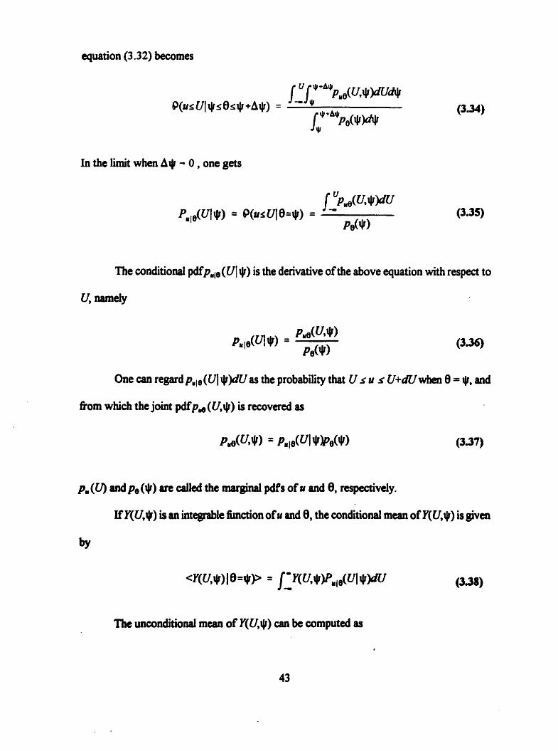
equation (3.32) becornes

In the 1 s t when A* - O , one gets

The conditional pdf'pa,,(Ul Jr) is the derivative of the above equation witb respect to

U, m e 1 y

ûne a n regard p,, , (Ut Ji)rm as the probability that

fkom which the joint pdfpd (Cl,*) is mvered as

IfY(U,g) is an integrable îunction ofu and 8, the conditional mean of Y(U,q) is given

The unconditional mean of Y(U,JI) can be cornputeci as

whae <Y(U,Jr) 1 is the conditionai expectation of the funaion Y((I,q), conditioned

upon the mdom variable 8.

In the next Chapter, terms such as <Y(U,@)b(B-@p, where 6 is Dirac's hction, wiu

ofien be encountered. These wiii k reduced following the above procedure as follows

Chapter 4

Mathematical Description of the Flow

4.1 The Velocity Field

4.1.1 Equation for the Means and Fluctuations

The Navier-Stokes eqwion appikd to a viscous, incomprhble fluid in the absence

of body forces is given by

and the continuity quaiion corresponâing to the conservation of mass is given by

where U, is the instantaneous local velocity, t is the tirne, xi is the Cartesian coordinate system,

p is the fluid density, P is the instantaneous pressure, v is the kinematic viscosity and the

indices i, j = 1,2,3 follow the summation convention.

Following Reynolds decomposition, one may decompose the instantaneous veiocity

and instantanaus pressure as

y. = q + u, ( 4 4

whac 4and P npresent the mean values of the velocity and pressure, respeaively, and u,

and p arc the velocity and pressure f l u ~ ~ t i o n s .

Substituting equations (4.3) and (4.4) in equation (4.1) and averaging the resulting

equation, one gets the mean momentum equation as

where U,U' is d e d the Reynolds (or turbulent) stress teasor (per unit mas).

The momentum equation for the vdocity fluctuations may be ob&ined by subtnaiag

equation (4.5) fiom equation (4.1) as

4.1.2 Balance Equation for the Turbulent Kinetic Energy

Turbulent kinetic energy per unit rnass is dehed as

An equation for this quantity is obtained by multiplying equatioa (4.6) by u, and averaghg and

omitting al vanishing tams as

4.1.3 Form of the Turbulent Kinetic Energy in USF

In stationary, uiiiformly sheared, neady homogeneous turbuienw, the velocity

components U2 and ü, vanish, the streamwist mean velocity Dl d e s in the transverse

direction x, only and the turbulence is nearly homogaicous in r, and x,. AppIying thcse

usumptions to equation (4.8) and omitting ail negiigibk tams (Tavouiaris and Co* 1981

8) one gar *

where E is the mean dissipation rate of the turbulent kinetic energy, quai to

4.2 Scalar Transport Equations

4.2.1 Instantaneous Scalar Balance Equation

Turbulence transports contaminants such as heat, chexnicd species and particies in

much the same way as momentum. Consider the transport of a passive scalar (for example,

tunpcratufe in flow with small amomts of heat SKI that the velocity field is not altend) in a

turbulent fIow of an cssentially constant density fluid. The c o d o n equation of such a

scilar rcquires that the total nte of change of the scaiar balances its molecuiar difFUsion, as

wbat y is the molccular dinusivity. Equation (4.1 1) describes the instantaneous temperature

field as weli as any othcr transponed passive scalar. Foiiowing Reynolds decomposition one

miy dccornpose the instantaneous velocity and tcmperahue as

whae and Ü. represent the mean values of the temperature and velocity, rrspectively, and 1

8 and u, designate the temperature and velocity fluctuations. Substitution of equations (4.12)

and (4.13) in equation (4.1 1) yields

a(T + e) - aT ae 87 + (U, + ux- + -) = y- 8 0 at

+ Y- ' 4 4 %% (4.14)

4.2.2 Balance Equation for the Mean Scalar

Ensemble avcraging equation (4.14), and omitting al1 vanishing fhichiating qmtities,

one may &tain the balancc aquation for the mean temperatwe field as

4.2.3 Balance Equation for the Scalar Fluctuations

The baiance equation for the tempersturr fluctuations is obtained by subtracting

equation (4.15) fkom w o n (4.14). The rtsulting equstion is

4.2.4 Balance Equation for the Scalar Variance

Mdtiplying equation (4.16) by 0 and averaging, one obtains a balance equation for

thc mean squared temperature fluctuations as

4.2.5 Balance Equation for the Scalar Variance in USF with an

Imposed Constant Mean Scalar Gradient

In addition to the rssumptions d e about the velocity field in USF, here it is asswned

that the scalar fluctuations arc homogencous in the x, and x, the mesn scalar varies lineariy

in x, and the mean temperature is n d y constant alone my strcadinc in the str-Wise

diredon (Tavoularis and Cornin, 1981a). Applying these approximations to quation (4.17)

and omitting the negiigiile tams yie1ds

The main wnciusion of these derivations is that, when comparing quations (4.9) and

(4.18), one notices that the balance eguations for the turbulent kincinetic energy and the scdar

variance are similar in form and, presumably, the velocity and the scdar field may evolve in

the sarne manner allowing for a wmparison between the state of the fine structure of the

scalar field to that of the velocity .

4.3 Pdf Formulation

4.3.1 The Scalar Pdf

Equation (4.17), the belance equation for the temperature fluctuation variances, gives

rise to non-closed tams, such as the turbulent transport tams. In this so d e d moments

formulrtion, these tams hvc to be moâelcd in order to solve the equation. Several models

aw&ited with this mcthod g a i d y rdy on gradient transport approxixnations. Ahhough

these models w a t s u d l in treating simple flows, such as passive scalar mixing in

homogcneous turbuierm, they were found to be inaccurate in trcating turbulent r&vt

fiows. Density variations and chernid d o n s in these fiows were found to be easiiy

recommodated in a pdfformulation and thc c l o m problem essociated with the pâfmeibod

is not mon Mcuit than that for a scaiar mixhg without reaction.

51

The method of derking a pdf conservation equation was iatroduced by Lundgren

(1967). Adopting Lundgren's technique, one can arrive at a wnservation equation for the

pdf of a scalar mixed by turbulence as follows.

First a *fine-grallied" one-point scalar probabiiity density fiinction, namely the scalar

pâfh one reaiization of the flow, is dehed as

where 8 is the Dirac hction ani 9 is d e d the sample space of the random variable 8(x,t);

the 9-space is also r e f d tu as the scalar or temperature space.

Then, the one-pint pdf is defineâ as the average of the "fine-graineci" pdfas

P ( 4 f ~ , t ) = wlJlf&P = W ( x , t ) - w (4.21)

4.3.2 Transport Equation for the Scalar Pdf

For the remahder of the derivation, p(j,x,t) will be denoted by p. Taking the time

derbative of equation (4.2 1) (Lundgren, 1967) yields

The last step in cquation (4.22) foliows because an infinitesimal change in 0 of de ha9 the

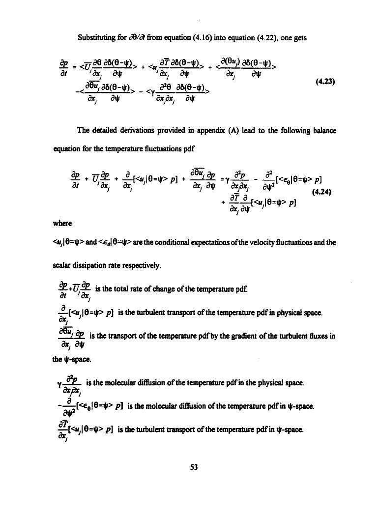
Substituting for dX3 fkom equation (4.16) hto equation (4.22), one gets

The detaiied derivations provided in appendix (A) lead to the foiiowing balance

equation for the temperature fluctuations pdf

<uI(-> and &I» are the conditional ucpectations of the velocity fluctuations and the

scaiar dissipation rate respedvely.

* +ù* ir the totaî rate of change of the temperature pdf. " jax, b[w, (0=p p] is the turbulent transport of the temperature pdf in physicai space. % a& ,-Lde is the transport of the temperature pdf by the gradient of the turbulent fluxes in *

y b the moleah dihion of the temperature pdf in the physical rpice.

*PX,

The lasi tenn acuiunts for the production of the Scalar by the action of the turbulent

velocity on the mean scalar field.

One should recaü that the tenn BU. in equation (4.24) cm be express4 in t e m of I

probabilities as

4.3.3 Form of the Scalar Pdf Equstion in Uniformly Sheared

Turbulence with an Imposed Constant Mean Scalar Gradient

To identify the tenns in equation (4.24) that arc to be meesured and assess th&

contnitions to the evolution of the temperature fluctuations pdf in this saidy, equation

(4.24) has to be impltmented for the temperature mixhg in a uniformly shesred turbulence

with a constant mean Aar pdient. In tbis flow configuration, one can invoke the flow

assumptions mentioned above. Then, &cf ominmg n@@bk trrms, the transport equation

for the scalar pdf, equation (4.24). reduccs to

At thU stage, it is important to point out thaî for a homogencous flow with a zen,

mean scaiar gradient., the scalar pdfevolves solely unda the efféct of the conditionai scrlrr .

dissipation. Equation (4.25) shows that for a sheared fiow with a non-zero ntean temperature

graâient, other terms, presumably with important effeas, enter the evolution equation of the

scalar field, mainly the lut term of equatioa (4.25) which represmts the production of the

d m fluctuations. Moreover, for an isotropie flow with a mean temperature graâient, the

second and third terms on the 1eA-hand side of equation (4.25) an absent which may suggest

that the scaîar pdf and the conditionai expectation of the sdar dissipation rate may evolve

differently in tbis fiow.

Chapter 5

Experimental Facility and Instrumentation

5.1 The Flow Facility

nie wind-tunnel (fig. 5. l), in which the experiments wae conducted was constructed

at the University of Ottawa and was descriied by Fachichi (1991). The flow of air was

filtered by fiberglas filtas (FM; mode1 KB-HE-40) and p d thmugh a diBi=, a settiing

chemkr icross which nirbdence rcducing screens were installed, and a 16 to 1 contraajon

A dKU generator wur instaiied imrnediately foiiowing the contraction (fig. 5.2). The shear

genastor comprised a set of 12 separate chiinnels, each 25.4 mm high, separated by

aiuminum plates, about 150 mm long. Screens with MIying rcsistances wcre attached uxws

clcb chuml so as to produce a uniforni sitar. A flow separator, consisthg of 12 pardel

plates, 6 10 mm long, aiigned with those of the shear generator, was insatecl into the flow

in order to make the large scaies of the flow unifiorm on the transverse plane. The test section

was 305 mm hi& 457 cnm Wde and 5 180 mm long. It providcd 4 dots for irisation of grids

and 0th- devices n o r d to the fiow direction. Probes were mounted on a traversing

mechanism providing transverse displacements with a minimum traverse of about 0.25mm.

The traversing mecbanism was attached to a hand-driven beh so that meawrements could be

taken at different meamWise stations. The side walls of the second half of the test section

diverged siightly to compensate for boundary layer growth. To increase the flow velocity, a

diffuser of 5" angle and a lmgth of 3 m was placed at the exit of the test section for some

tests.

5.2 Heating system

The hcating system, show in fig. 5.3, consisteci of a wooden fhme that could be

insateci n o 4 to the flow h o the dots provideci in the wind-hmnd test section. Across the

verticai w d s of the fiame, 47 heating elements (Nicrome 60) wae stretched. The heaîing

dunents were 0.8 mm wide, 0.08 mm thick and 6.3 mm apart and w m heated in pain by

variabie voltage sources to producc the desircd initial mean temperame profile. The heating

dements wae kept stretched using s p ~ g s attached to th& ai&. The heating system was

introdud into the flow at a distance of 0.61 m upstrcam of the fint test seaion (fig. 5.4) to

aiiow for higher temperature vari- dowasatem in the test d o n . A copper hcating p k

was mounted inside the top of the wind tuwl to prevent hcat losses and to d o w for kna

transverse homogeneity of the tmpaihirr fiuctuations.

5.3 Hot wire instrumentation

In the present work, several hot win probes, all having tungsten senson of 5 pm

diameter, wae used. These included single hot wires (DANTEC mode1 55P14) with nomid

lengths of about 0.6 mm, which were used for one-point, streamwise velocity m m e m e n t s

and a pair of single-win sensors, with nominal lengths of about 0.9 mm, mounted on a

travershg mechanism (fig. 5.5) for two-point, streamwise velocity measurements. The

travershg mechankm included two micrometers h a h g a 0.01 mm precision, used to phcc

the two hot wires probes nonnal to the flow at the desired transverse separation distances.

A specially made, paraüel-wire probe (AUSPEX), with two sawrs having a nominal length

of about 0.9 mm and separatcd by a 0.6 mm distance, was used for the measurunents of the

transverse derivatives of the streamwise velocity. Simultaneous measurements of the

saeamwise ami the transverse veloQty wmponents were done using a speaally d e probe

(fig. 5.6) ~onsisting of two-subminiature cross wires having a length of 0.7 mm and a cdd

w k of b u t 0.5 mm. Eacb pair of d e s wu scparated by a nominal distance of about 1 mm

It was rrallltQ however, tbat the cold wire signal was contamulated by the heat conduad

fiom the cross wins to the probe body. For Uns remon, the cold win on the tbrec-wire wp9

not used in the finJ rn- but a special probe holder wu designcd on which au

independent cold wirc was mounted in the vicinity of the cross wires at a distance of about

1 mm. In the heated flow, the cold wire signai was uscd to CO- the hot wire outpits for

thQt tanpenture sendtivity.

The hot wins w a e opcroted in a connant tanperanirc mode by a muiti-channd I

memorneter unit (AA Lab Sys, mode1 AN-1003). Each channe1 had built-in low pass filters

with ait-off fiequencies ranging fiom 380 Hz to 14 kHz, built-ii signal conditioning,

consisting of amplifiers with gains ranging fom 1 to 20 and DC voltage offsets fiom - 12V to +12 V, and a tiequency compensation unit to d o w for optimal fiequency response of the

hot wins. When higher cut-off fiquencies were rquired, the anetnometa's filters were

bypasseû and homamade filters, based on the second order Buttemuorth design (fig. 5.7).

were used. The hot wires were calibmted in the wind tunnel against a pitot tube. The

difference between total and static pressures was measured with a pressure transducer that

was calibrateci against a Maiem micromanometa.

5.4 Temperature Measuring Instruments

Thermistors were used to measurt the mean temperature of the heated fiow. These

wen giass-coated, mini-probes ( F e n d Electronics, 2000 Cl), opefated by a home-made

clecüonic circuit which could provide individual signals as well as direct measurements ofthe

temperature Merence by subtnaing the coaditioned outputs of the thermistors (fig. 5.8).

The thenniston wae caiiirated in the caiibration jet agsinst a merwry thamorneter with a

O. 1 K precision.

In the heatd flow, cold wirc (1 Cm diameter, 1 Wh Platinum) probes w a e used to

m m temperature fiuctuations. A single cold wire of about 0.5 mm in length was used for

the one-point measurcments of tanpenture fluctuations. A set of two cold d e s , Ymilar to

the one medoneci above, wae mountcd on the travasing mcchanism describeci in section

59

5.3, and the spacing between the cold wires was adjusied to the desired distance for two-point

temperature fluctuation measurements. Simultaneous measurements of velocity and

ternperature fluctuations were paformed with the txiplewire probe describeci in section 5.3

using the independent cold wire. AU wld wires were operated by a home-made electronic

circuit (fig. 5.9), cornprising a constant m e n t source, low-pass fiiters with a>toff

âequencies that could be selected at 1,2,5 and 10 and ampiifiers with selectable gains

of 1000,2000,5000 and 10000. The ciraiitry was DC powereû by batteries to minimire the

contamination of the signals by the 60 Hz line fieguency.

5.5 Calibration Jet

Caiibrations of thermistors and cold-wires and measurements of directional and

tanpefature sensitivities of the hot-wires were made in a calibration jet (DIS4 mode1

55D9û). Compressed air fiom the supply iines was fed to a pressure wntrol unit (DIS4

mode1 55D44) der which it p a s d through an air filter, a pressutt regulator and a sonic

wnle to produce a steady, constant flow rate. The flow then passed through screens and

fiow straighteners before uciting through an axisymmetric nozzle. A homemade, motor

driva probe positioning systan was added to the unit. The jet au temperature was rdjusted

by a h o m e d e electnc heating system, which was installed before the jet unit. A swiveliing

mechdm rotating in two perpendicufar planes was ins&lled at the exit of the jet nozzie for

m e m e n t s of îhe hot wire directionil sensitivity.

5.6 Data Acquisition System

Raw analog signals obtained fiom the meaairing instruments were digitized using a

1 &bit dog-to-digital converter (IOTECH, mode1 488/I 6) with analog input voltage ranges

sdectable as *1 V, SW, *5V and *10V. Up to 16 sngle-mded or 8 differential analog

inputs could be sampled shuftaneously at a ssmpling fiequency of up to 100 lcHz per

chamel. The d ig i t id data were transferred to the hard disk of a penod amputer and then

transfied to a CDROM for long term storage.

5.7 Digital Filtering

Non-recursive digitai low-pas nIters were designeci to fiuthm eliminate the

undesirable high frequency noise part of the probe signals. These arc known to have a zero

phase shüt and t h y presave the signal waveform up to the desired aitoff fiequency.

Therefore, no mors are intrduced in estimating the skewness and flatness of the original

sigrlai (Tavoularis and Consin, 1981 b). A low pas% non-rtcufSive digital filter was

constructeci as

where y, and x, arc the output and input signais rnd b, and b,, am the Fourier coefficients of

the filta's d e r Gnction, de- as

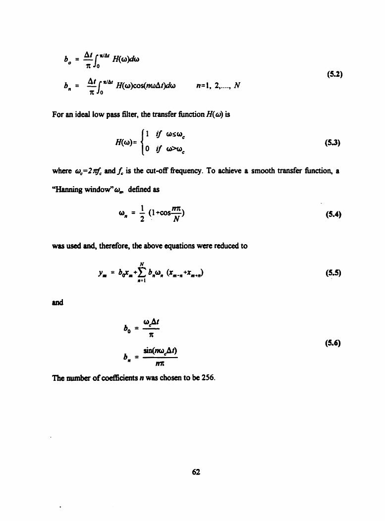
For an ideal low pass filter, the tramfa nsferction H(o) is

whcn 0,=2 I& and f, is the cut-off &equency. To achieve a smooth tramfier huiction, a

"Hannllig window"~, defined as

was used and, thdore, the above equations were reduced to

The number of COCf]6icients n was chosen to be 256.

Chapter 6

Measurement Procedure and Resolution

6.1 Calibration of the Hot Wire Probes

Hot wire anemometry has ban used extensively in measwcments of mean velocities and

vtloaty 0ucRiations in turbulent air fiows. A hot wire is a thin cylinder, which is heated

clcctrically. In the piesencf of a fiuid flow, the rate of heat transfm &om the wire varies in

rcsponse to changes of the instantanwus velocity of the fiow. This can k rdated to the

instantaneous changes of voltage across the hot win through the weîl kmwn 'Xing's hwm.

A modified saniunpirical form of mg's law is

E2 = (A + BU"XT" - Td (6-1)

where T, and Ta an the tanparturcs of the wire and of the flow, respectivtly, U is the

tous flow vdoaty normal to the wire and A, B and n arc constants to be daermined

Born calibration. E is the voitage output of the constant tanpawrre bridge, represcntiq the I

voltage across the hot wire, and is given by

E = iR, (6.2)

where i the w m i t flowing into the hot wire and R,, is the wire operating resistance to be

chosen such that the wire temperature T, is about 473 K, which is maintained constant in the

constant temperature mode by a feedback circuit. The choice of R. can be determined â.om

the hear relationship between the wire resistance and its temperature as

R, = Rail + aJT,-QI (W

whcre ais the wire resistivity obtained by measuring the resistance of the hot wire at diffèrent

temperatures (see fig. 6.1 for a typical R-T ref ationship).

CJibrations of single wires were obtained by plecing them in the unobstniaed tunnel

in which the turbulence intaisity was lower than OS%, in the vicinity of a pitot tube and

normal to the flow. Plots ofthe outputs fiom the hot wires and the pitot tube were then least

square fined accordhg to equation (6.1) and the aponent n was optimized to yield the

minimum r.m.s. mor deviation tiom the fitted data

In the cross win amangement, w b both wires are inclined with respect to the flow

(fig. 6.2), an effdve coolhg velocity, U # is dehed as the hypotheticd flow velocity n o d

to thc wire that wodd produce the same coohg as the a m a i fiow vekity. This vdocity is

where U, V and W are the inptantaneous velocities defimd with respect to the probe axis su&

and Wis normal to the plane of the h s . 8, and 8, are the wire inclinations with respect to

the probe axîs. When the probe is aligned approximately with the mean flow direction and the

turbulence intedty is small, one gets

CI6 = Usine, - vwse,

U' = usine, + vcose,

The dbration jet was used to experimentaüy detamine the orientations of the cross-

wires. This was achieved by varying the angular position of the cross-wire probe with respect

to the jet a i s (fig. 6.3). An expression relating the jet inclination with respect to the probe

wis p and the hot win aagles 8, and 8, wss denved as

where is the jet veloaty. For each jet inclination cp, 8, anci O2 were evaluated using

cquation (6.6) and average values of 8, and 8, wen found to be 42.15" and 9-23'

respsctively for the s p d c probe used. These values m measurably diffenat fiom the ideal

* 4 5 O .

The m d e d King's law for the two wires leads to expressions for the eEéctive

cooiing velocities Us and II', as

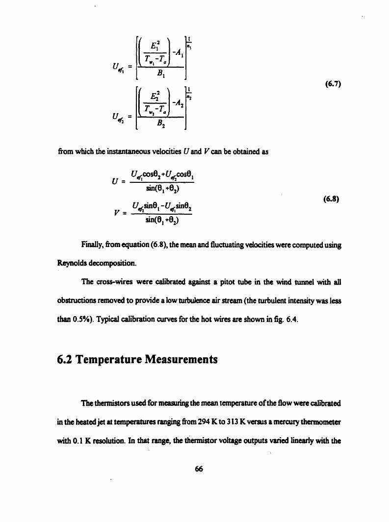
fiom which the instantaneuus velocities U and V c m be obtained as

F S y , fiom equation (6.8). the mean and fiuctuating velocities were cornputeci using

Reynolds decomposition.

The cross-wires were calibratecl againsi a pitot tube in the wind tunnel with ail

obstnictioiw removcû to provide a low turbuîenct air Stream (the turbulent intensity was less

tban 0.5%). Typid diration curves for the hot wins an show in fig. 6.4.

6.2 Temperature Measurements

The thCrmistors used for meamhg the mean temperature of the fiow were calibrated

in the heated jet at taapaatures ranghg âom 294 K to 3 13 K versus a merairy thnometer

with 0.1 K rrsolution. In that range, tht thennistor voltage outputs wied linearly with the

mean jet temperature. Typicd calibration curves for two themistors are shown in fig. 6.5.

Temperature fluctuations were measured with the wld wires describecl in the previous

Chapter. A s y s t d c study was conducted to determine the maximum m e n t intensity fed

to the cold wires at which the sensitivity to mean velocity changes was negligible. It was

f m d that a cment levei of about 0.4 mA, the cold wire showed no apparent sensitivity to

the mean velocity (fig. 6.6) . The mld wires were calibrated in the heated jet against a

previously calibrated thennidor. Typical caiibration ames of the cold wires are shown in fig.

6.7.

6.3 Resolution

A turbulent flow contains motions of different scales which may be characterizeû by

the integral Iength d e , representing the typid slle of the most energetic eddies, the Taylor

miaode, which rnay be lwsely regarded as the threshold scale, at which the dissipation of

turbulent kinetic energy becornes significant, and the Kolmogorov microscale, reprtsenting

sizes of eddies atinly domllrated by viscous actions. To study the fine structure of a

turbulent flow, the wire size anci its fiequency respnse must be chosen such that it ~CSO~VCS

saks comsponding to the Kolmogorov microrcrk.

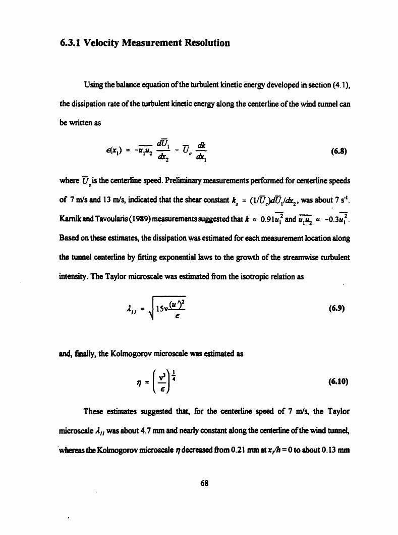
6.3.1 Velocity Measurement Resolution

Using the balance epuation of the turbulent kinetic energy developed in section (4. l),

the dissipation rate of the turbulent kirietic energy along the centerline of the wind tunnel can

whae Ü is the centeriine speed. Prebimy me C

asurements performed for cen

of 7 mls md 1 3 mls, hdicated that the shear constant k, = ( I lÜE)dÜ,/di2, was about 7 se'. - - -

2 KMUkandTavoularis(1989) m ~ e r n e n t s mggesteci that k = 0.91 u: and up, = -0.3u, .

Based on t h esthates, the dissipation was estimateci for each measurement location along

the tunnel centerlim by fitting exponentiai laws to the growth of the streamwise turbulent

intensity. The Taylor microsde was estimateci fkom the isotropie relation as

anâ, M y , the Kolmogorov miaoscaie wu Cssimated as

These estimates suggcsted that, for the centerline speed of 7 m/s, the Taylor

microscale A,, was about 4.7 mm and nedy constant dong the cenferline of the wind tunnei,

. w W the Kolmogorov microsde q d e c r d fkom 0.2 1 mm at xJh = O to about 0.13 mm

- at xJh = I l . Accordingly, the Kolmogorov fiequency, f i = U J ~ Z ~ , hcreaseû fiom about

5.5 kHz to 8.7 kHz. For the centerline speed of 13 mls, A,, was nearly constant, with a value

of about 3.4 mm, qdecreased fiom about 0.14 mm at xJh = O to about 0.08 mm rJh = i l and

f, increased fiom 15.5 lcHr to about 25 kHz.

6.3.1.1 Spatial Resolution

Clearly, the 0.6 mm long single hot-wire is much larger than the estimateci

Kolmogorov scales reported above and it may introduce some erron in measurements of

quantities related to the fine structure. Howeva, a M e r decrease in the wire length

introduces otha aron due to heat conduction to the prongs and to non-uniform heating of

the Win. Plots provided by Wyngaard (1969) suggested that, for = 7 m/s, C

would be underestimated by 5% at xJI, = O to about 10"h at x/h = 11 and, for the case of 13

m/s, t would be underestimated by 10 % at xJh = O to about 20 % at xJn = 1 1 . The above

esthates indicate that the rneaswed stremwise Taylor microscale would be ovaestirnated

by les that 100A in the worst case.

The strcanwise velocity derivaîives wme duated ushg Taylor's "âozen fiow"

hypothcsîs which may k applied in low turbulent intaisity Oows. Heskestad (1 %5) provided

an approximatc correction to the streamwise velocity derivative when Uivoiced ftom its

temporal couterpart as

In this particular study, the highest turbulence intensity was U#üc= 16%, for the case with C

= 13 m/s and at xJh = 1 1. Using the fact that, in this partiailar flow, 24,' = 0 . 6 5 ~ ~ ' and u,' p.

0.5u2ii,: then the above equation suggests that the maximum error in estimating the mean

sqwed streamwise denvative ushg Taylor's approximation, would be less that 4%.

For the transverse velocity derivatives, the parailel wires had a lengrh of 0.9 mm and

wae spciccd by a distance of 0.6 mm. The wire lmgth was chosen to be larger than the siagie

wire used for the one-point measurements, b s e , according to Wyngaard (1969), an

incrase in the length of the wires can only improve the transverse derivative measurements.

According to the estYnates of Wyngaard (1969), (hl/&$ may be underestimated, forD

= 7 ais, by 10"/. at xJh = 0 to about 20.h at xJh = I l , and forüc = 13 m/s, it would be

undmestimated by 2W at x,h = O to about 35% at x f i = 11.

In view of the above, spatial corrections to (& ,/&,)2 and (&,/ax,)2wïU be applied

according to the m e h d of Wyngaard (1969). Unfortunately, there are no avaiiable mcthods

to correct the skewness and flatness of the sireamwise and transverse velocity derivatives.

But, Daksai and Azad (1983) estimated the skewness, S, , , and flatness, F, , , of the I t 1 t

strcamwise velocity derivative obtained fkom signais of hot wires of di&rent sizes in a

turbulent bounâary layer and suggested that S' , and F, , wen neariy invariant 4th the I I I l

hot wim length, I , for 2.9CIJF20. Moreover, Garg and Warbaft (1998) showed thst the

measured transverse derivative skewness, S,,+, maintaineci neariy a constant d u e for up

to Aqq= 10.

6.3.1.2 Temporal Resolution

The above cstimates suggested that, forDe= 7 m/s, the maximum Kolmogorov

fhquency, f, was about 8.7 W. The Nyquist criterion depicts that the sampling fiequenq

should be at Ieast 17.4 kHz. Accordingly, the signals fiom the single wire and the paraiiel

wires were low-pass fütered at 14 lEHZ and sampled at a rate of 50 kHz. For Üc = 13 mis,

the maximum& was about 25 kH& the signats fiom the single wire were low pass Ntered at

a âepuency of 38 kHz and sampled at a samphg fiequency of 100 kHq but to conform with

the samphg bequency limitations of the analog to digital converter, the signals fom the

pardel wires were low-pass nItered at 25 IiHz and samp1ed at a sampling âequency'of 50

kHz. About 100 records, eadi consisting of 400 000 data points for the single wke and 262

144 data points for the p d e l wires, were sampled. Each record had a duration of about 5

seconds correspondhg to roughly 800 times the integral tirne scale which cnswed g o d

statisticai representation of the large d e s of the flow.

6.3.2 Temperatun Measnrement Resolution

The heating systcm was insatecl into the flow at a position about 0.61 rn upsmm of

the test @on ta aîlow the dmlopment of relatively kgh temperature fluctuations in the test

section. nie possible &ects of the heating system on the velocity field were investigated. To

ichieve mutsurable tclllpmturt Merenccs and to avoid elexnent viirations, one had to

. * muntsiii the c«rt«iine s p a d below 7 d s . At the centeriine speed of about 6.6 m/q a

constant mean temperature gradient &?/k2of about 7.8 K/m was produced at rJh = 0.5.

Under these wnditions, the Taylor microscale was estimated to be about 5.2 mm and the

Kolmogorov microscale was found to decrease from about 0.20 mm at x/h = 3 to about 0. 16

wn at xJn = 8. The Consin-Obukhov microscale, correspondhg to the dissipative scales of

the temperature variance and defined as va= QryWq, decreased f?om 0.26 mm to about 0.2 1

mm at the locations mentioned above. Accordingly, the Kolmogorov firequency for -

temperPhinfk = UjZx rl, iacreaseû nom 4 kHz to about 4.9 W. The rate of destruction

of temperature fîuctutioas was estllnated &om the balance equation (4.18) using an

exponentid fit to the growth ofpreliminary measurements of the temperature variance dong

the centeriine. Then the Cornin microsde was estimated using the isotropie expression

to be &out 3 mm and nearly constant dong the wind tunnel centeriine.

6.33.1 Spatial Resolution

Whai using the 0.5 mm long cold wire, ( a e / & ~ ~ w d d be undercstimatcd by about

1 O./ (Wyngaard, 197 1) and as a muiî, the Corrsin microscale, A, , would be overestimated t

by about 5%. Browne and Autonia (1 987) conducted an experimcnt to study the dect of the

cdd Win length on the statistics of the temperature fluctuations and th& derivativcs. Thy

suggested that, to cradicate the effects of end conduction on these statistics, the cold wire

must have a length to diameter ratio l / a larger than 1 5 W. For d, = 1 prn, IJd, = 1500

nquins a win with 8 length of 1.5 mm, whkh wodd d t in M =or in of about 38% in

72

estimating 12 (Wyngaard, 197 1). Further nducing the diameter of the cold wire to I

increase I J 4 . would make it very fragde and extremely hard to handle and repair. Mydlmky

and Warhafl (1998) commentesi that the spatial resolution of the cold win has the

predomlliant ambution to the unartaitity in estimating temperature derivative statistics and

uscd a cold wire with /,,hi& of about 560. In view of this, the present choice of IJci, = 500

seemed to be reawnable for this type of study.

Th îransvasc temperature denvative, a/&, and diaerences, Ae(x3, were measured

by placing two cold wires of neariy the same length and resistance on the traversin8 system

d e s c r i i in section (5.3) in the heated flow parailel to the mean temperature gradient,

dB&3. The cdd wires were sep-ed by a distance, 4 of about 0.5 mm for the transverse

derivafjvt estimate. Thedore, d q B would Vary fiom about 1.9 to about 2.4, which are in the

ranges of d/q8 niggested by Antonia and Mi (1993). Anselmet et al. (1994) and Tong and

WuhPff (1994).

6.3.2.2 Temporal Resolution

According to the above estimates, the maximum Kolmogorov frequencks for the

velocity and temperawe were 4 IuIz and 4.9 kHz respectively. To satidy the Nyquist

criterion, the cross-wirc signais wae low-pas filterrd at a eut-off fiequency of 8 IcHq the

wld wire si@ was low-pass filtaed at 10 kHz and all signals were sarnpled at r fiqucllcy

of 20 kHz The sunpled cold win signals wae fiirther low-pass fihered using a digital 61tm

(section 5.7) at a nitoff fiepuency of5 kHz pnor to processing. At this cut-off fnsuency,

the sipal-tonoise ratio, 3/d, whcn n iP the coid wire signal in the unheated fîow, wied

73

fiom 47 to about 90. To aisure good &&tical representation of the large scales of the flow,

60 records of 262 144 data points were colected.

Chapter 7

Measurements of the Fine Structure of the Velocity

Field

7.1 The Mean Velocity Field

Mmernents of velocity derivatives d structure fùnctions wen conductecl at two

mean ccnttriinc velocities, 7.3 mls and 1 3 .O m/s. Ihe latter caitaline speed was achieved by

inff;illine a diniiser u the exit of the wind m e 1 test section, as described in Section 5.1.

M- wae pdonned at positions correspondhg to r/f, = O, 2,4,6,8,10 and 1 1,

whae h U the wind tunnel hu& equal to 0.305 m. Fig. 7.1 shows typid transvetsc profiles

of the mean vtlocity ü, . Thesa CXhl'bited good lincarity accept at fhr downstream distances

whae the e f f i of bouaduy laya growth on the waOs of the wind tunnd wae noticeable.

Fis. 7.2 dispiays the &eu constant k, = s/ÜC d Ü , / 4 , for cich cniterhc rpced and a the

streamwise positions mmtiond above. This plot suggests that k,uprap roughly constan! and

75

e q d to about 7.07 0.19 mg', independen* of the centerline speed and ofthe streamwise

position. This also shows that the addition ofthe diiser had no signifiant effect on the value

of k,.

7.2 The Turbulent Stresses

Fig. 7.3 shows transverse profiles of the streamwise r.m.s. turbulent fluctuations. The

obsaved variation in U[/Ü hcreased with increftsing centerline s p a d and downstream C

position. At its worsc, near the tunnel ait, the variation was les than 30 % in the core of the

winâ tunnel; thus, the flow may k 8ssumed to be nearly homogeneous in the transverse

direction. The downstream dewloprnent of the turbulent stresses for both ccnteriine speeds

is shown in fig. 7.4. Exponential fits ta the data gave, for = 7.3 ds, c

which are within 5 % from cich other. The rneamred Taylor microsde, A,,, turbulent

Ryndds number, Re, and Kolmogorov microde, q, are provided in table 7.1. The s ~ i e

table provida the nubulenî hetic cnergy dissipation rate.

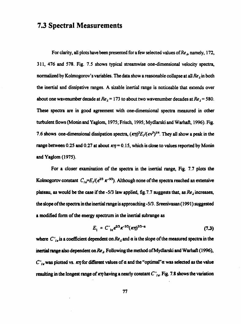
7.3 Spectral Measurements

For clarity, aü plots have k e n presmted for a few selected values of Re, namely, 172,

3 1 1, 476 and 578. Fig. 7.5 shows typicai strmwise one-dimensional velocity spectn,

nonnalized by Kolmogorov's variables. nie data show a reasonable coilapse at aiî Re, in both

the inertial and dissipative ranges. A sizab1e inertiai range is noticeable that extends over

about one w a v e n m k decade at Re, = 173 to about two wavenumber decades at Re, = 580.

These spectra are in good agreement with one-dimensional spectra measured in other

turbuient flows (Monin and Yagiom, 1975; Frisch, 1995; Mydlarski and Warbft, 1996). Fig.

7.6 shows ont-dimerisiod dissipation spaPa, (q)2EJ(N')V4. They al1 show a peak in the

range betwecn 0.25 and 0.27 at about q = 0.1 5, which is dose to vahies reporteci by Monin

and Yaglom (1 975).

For a closer examination of the specûa in the inertial range, Fig. 7.7 plots the

Koimogorov constant C,,=El/(I( K-~). Aithough none of the spectra reached an extaisive

platau, as woukl k the we ifthe - 5 0 law applied, fig.7.7 suggests thah as Re, increases,

the dope of the spectra in the inertial range is approaching 4 3 . Srdvasan (1 99 1) suggested

a modifieci fom of the enagy Jpeanim in the inertial subrangc as

El = C',,PK-~'(*-= (73)

whae C 'Js a coefficient dependait on ReA and a is the dope ofthe measured spectra in the

hathi range dso dependent onRe,. Following the method of Mydlarski and Werhaft (1 9%),

C ',,was plottcd W. q for différent values of a and the uoptirnalwa was s e l a d as the value

d t i n g in the longest range of q having a neariy constant C ',, Fig. 7.8 shows the vaxiation

of the "optimal" values of 5 / 3 4 , which rnay be fiîted by the curve 120Rei'~. The optimal a

M e r d fiom the Kolmogorov value of 513 by 8 % at Re, = 300, by 5 % at Re, = 480 and

decreaseâ to 3 % at the highest Re, = 660. Fig. 7.9 shows sample plots of C ;, as a bction

of q. For Re, larger than 480, these values are close to values reported by Monh and

Yaglom (1 975). Sreenivasan (1 995) and Mydlatski and Warhafl(1996) at comparable Re,

and supports previous findings, that C ',, approaches a constant value as Re, inmeases. For

cornparison, C;,= 0.70 at&= 3 0 , C',,= 0.65 at Re, = 480 and C;,= 0.60 at Re, = 580.

7.4 Velocity Derivative Statistics

F i the pdf of the norrnalized streamwise velocity fluctuations are presenteû in fig.

7.10. These are n d y Gaussian with a skewness of -0.04 and a flatness of 2.91.

Fig. 7.1 1 is a plot of the ratio ( ~ , J ~ , J ~ / ( ~ ~ / ~ $ . The variances of both velocity

partial derivatives have been ~rrected for the wire length and wire m g using Wyngaard's

(1969) estirnata. This ratio, plotted for both centerline speeds, fluctuated betwecn 0.45 ad

0.55 for Re, incrcasing fkom 140 to 660 . This ratio is close to the l d y isotropie Mhie of

0.5, but substantiaUy brger than the value of 0.22 rrporied by .Tavoularis and C o d (1981

b). The rasons for this dieraice have yct not yet been identifid.

In contrast to the pdf of the velocity fluctuations, the pdf of the streamwise vdocity

daiv&e are highly non-Gaussian, as demonstrated in fig. 7.12. For aU Reynolds numbers

-cd, inctuding cases not shown in fig. 7.12, the pdf of ib /a, displaycd two main

W. Fdy, th& tails are v a y broad and neariy cnponentiai in form, becomin8

78

progressively steeper as Re, increases, with the negative tails being more flared than the

positive ones. Secondly, the peaks of these pdf semi to shift toward positive values of di/&,

and to becorne sharper as Re, increases. The sharpness of these peaks is an indication of

intennittency of the fme structure and consistent with the expectation that the internai

intermittency increases as Re, inmeases. Because the tails of these pdf are associated with

iarge and rare fluctuations of di& ancl, hence, with the dissipative sedes, their distribution

would indicate the degree of intermittency of such scales. Their tails rnay be fitîed by the

aponential expression

where z, = (&,/&,)/(&t,/&,)'. Fig. 7.13 shows that values of P, detennined fkom the

positive tails were somewhat higher than values determineci fkom the negative ones, but both

showed a monotonic decrease with Re,. The systematic decrease in P, as Re, increases is

consistent with the acpe*ed increase in the intanal intermjttency. Figs. 7.12 and 7.1 3 clearly

show tht the asymmetry of the pdf of the streamwise velocity derivative becornes more

p r o d as Re, increases. This aqmmetry may be better seen in fig. 7.14 in which the pdf

have been rnuitiplied by the cube of the nonnalized derivative.

Figs. 7.15 and 7.16 show the measureâ values ofthe skewness S'/a, and the flatness

F ~ 1 4 of the streamwise veiocity derivative for differait Re, at two centeilllie specûs, - U, = 7.3 mis and vc = 13.0 d s . Aithough the trends are similar for both cmteriine

spϞs, the magnitudes of the mecisureci Sa,,, and F4 la, do not collapse. This may be

p d y due to acperimtlltal mors and partly to maIl diffetmces in the large d e s of the flow.

As rceri in fig. 7.15, the rneamed skewness SA, ,& U non-tad and negative. Note that a

79

non-zero Sc41ih, is not a violation of Kolmogorov's similarity hypothesis, but its non-

constancy for dinerent Re, would be (F~isch, 1995). Fig. 7.15 shows that Sal,,, varies only

slowly with Re, increhg fiom about 0.3 7 to about 0.43 in the range of Re, between 140

and 660. The measured skewness falls within the range of data collectai by SrraWasan and

Antonia (1997) fiom numerous experimental and numerid studies. A power law fit to the

present data suggested that S' ,&, varies as Re?'. The exponent O. 1 is not far fiom the value

of 0.07 obtained by Frisch (1995) fiom the measwements of Gagne (1987).

C O ~ P ~ t0 sa! lai , F4,at shows a stronger dependence on Re, and inmeases with

kcreasing Re, (fig. 7.16), ~&aait with the faa the intemal intermittency should Uicrease

as Re, inmeases. The measwed F ,,,, , which incteased fiom about 5.5 to about 7.7 in the

range of Re, untestigated in this study, falls within the range of various measurernents

rcported by Sreenivasan and Antonia (1997). A fit to the data of fig. 7.16 suggested that

Fd,/al varies as Re;''. The acponent 0.1 8 is close to the values obtained by Frisch (1 999,

namciy 0.15 Born the data of Anselma et al. (1 984) and O. 18 h m the data of Gagne (1987).

Up to this point, it has been shom that, for the range ofRe, studied, the reported pdf

and the statistics of the strearnwise velocity derivative a/&, are consistent with numaous

acpaimental and numerical studies. No cornparison was made with the measurexnents of Garg

d Wuhaft (1 998). beuuse theh messund S'/& and F~~~~ showed considaable scitta

and no systetnatic tnads with Re,.

Nact, the focus wül k on the transverse velocity derivative statistics. Fig. 7.17 shows

the pdf'of bJcZr, at ththe same Re, as those used for the pdf of &{ch,. Some featurw found

in the pâfof Lù /a,, in partja~iar the acponartiai tails and the hcnasing sharpness of the

perL as Rr, incrtsscs, are Jso mcountered in the pdf of et /af. However, thac are rlso

80

some Merences. The positive tails of the pdf of dr JaL, are more flared than the negative

ones, the peaks of these pdfare sbifted towards the negative values of drJ& and the shape

of the these pdfbecornes more symmetricai as Re, inmeases. Exponential fits to the tails of

these pdf using the expression

P(ZJ = e (7-5)

where z2 = (du,/&2)/(&,/&2)', provided /î" for the negative taiis which were higher than

those the positive taiis (fig. 7.1 8). A decrease in /?., wit h increasing Re, was also noticeable,

but not as pronounceci as the increase in the exponent P, . The asymmetry of these pdf may

also be seen in fig. 7.19 which shows that the positive peak was always higher than the

corresponding negative pcak in the range of Re, shidied and, to a lesser ment, that the

asymmetry seems to kcome les pronounccd as Rc, inmeases. The measweû skewness and

fiatness of /a2 are showi in figs.7.20 and 7.2 1 respectively. Along with the presmt

measurcments of SAl ,4 , the dues measured by Tavoularis and C o d (1 98 lb), Garg and

WamaA (1998) and Runv (19%) were also included. As show in fig. 7.20, the vaiues of

&,,4 were positive for the range ofRe, reported in this study. The signs of the skewnesses

of a/&, or aL{ik3 have beai atplained by the phenomenological mode1 of Tavoularis and

Corrsin (1981 b), accordhg to which, for positive au&, a "mplike" structure of u,

ddops, causing SriiI4 to k ncptive and SaI,* to be positive. Note that, rccording to

this rnodei, the presence of non-zero mean velocity gradient is essential for a non-zero

% lai . Ttgs was confinned by Ferchichi and Tavoularis (1 998) who measured a neariy zero

sLla, Us grid-gaicrated turbulcilct.

Since a wn-zao S4,&, is aot inconsistent with local lsatropy hypotheses, then

$1

Sal,+ would be a bmer meanire of deviation nom local isotropy. Fig. 7.20 shows that

SA,,, decreases &om about 0.7 to about 0.34 as ReA inmeases fiom 140 to 660, indicating

that the fine structure may be tending towards local isotropy. The main conclusion hae is that

the skewness of &/a2 evoives d i f f d y with Re, fiom the skewness of A/&,: the latter

increases with increasing Re, while the former decreases. Fit to each set of data suggested

that, &,,a2 deaeased roughly a s ~ l t O l , which is consistent with Garg and WarhaA (1 998)

result. It is important to mention that the change in sa,,, is quite significant (almost

reduccd by haif for Re, verying form 140 to about 660), and that its dependence on Reynolds

number c m o t be accounted for by experimental uncertainty.

Fg. 7.2 1 displays the measured flatness of the transverse velocity derivative F' ,k2 ,

together with the values obtained by Tavoularis and Comh (1981 b) and by Garg and

WarhaR (1998). The m-ements of the latter authors indicated that F', decreased as

ReA increased for low vdues of Re, but for the highest Re, considereâ, seaned to

approach a constant. The presait me8suTements seem to suggest that F wnsistently 4 l a 2

increases with Re, but at a dower rate t h F'',&, does. A power law fit to the data

was F4,4 a ~ e ? ' , aithough a power law rnay not be appropriate in this case, aa the data

in fig. 7.21 show that F,, tends towards a constant value.

7.5 Inertial Range Statistics and Structure Functions

Figs. 7.22 and 7.23 are plots of the pdf of the strearnwise and transverse veloaty

diflFerences Au,(x,) and Au&), rr~pecti~ei~, at Ro, = 578 for r/q = 2 1, 76, 142 md 2 1 O (r

is the sepmtion distance measuied in the x, or x, directions). These figures show that, for

srnall separation distances, the pdfhave extendeci taiis, sllnilar to those seen in the derivative

pdf; but, at larger r/q, they approach the Gaussian shape. It is interesthg to see that, for the

pdfof Au,(x,), the positive tails decay faster towards the Gaussian than the negative oms do,

whiie the opposite can be observed for the pdf of Au,@,).

Fig. 7.24 is a plot of the nomialized second order longitudinal velocity structure

function~&,,(x,)l(r&'~ asafbnctionofr/qforRe,=172,311,476and578. Inconfonnity

with the normalued spectra shown in fig. 7.9, fig 7.24 shows that the inertial range widens

as ReA increases. For the highest Re, examine4 the normalized second orda structure

hction seans to suggest that the Kolmogorov constant C, is about 2.2, close to the dues

of 2.25 report4 by Boratav and Pelz (1 997) and 1.95 reporteci by h i m e t a al. (1984). but

sommhat higher thm the d u e of 1.85 reported by Garg and W a M (1998) for a lowa

Reynolds n m b a . Sincc C, = 0.76C, (C,is the Kolmogorov constant for a thrœdimensional

spectnun) and Cl. = 0.327Cr (Monin and Yaglom, 1975). the prcsent value of C,=2.2

suggests that C,,=û.55 consistent with the vaîue of C,,of about 0.6 nporteâ in S d o n (7.3)

ut the same Re, = 578. Showa in fig. 7.25 is the no& second order transverse velocity

structure bction D', ( x i ) / (FE)" . AiAltugh the number of data points plotted was not

as iargt as that for the longitud'd velocity structure hction, the data sean to indi~iitt tbat

D:, (x,) / ( ~ 8 ) ~ reached n d y a constant value of about 4 in the inatial range. Note that,

at Re, = 3 1 1, this valut is about 3.5, compared to the value of 3 .O reported by Gug aiad

Warhaft (1998) at nedy the same Re,.

Fig. 7.26 is a plot of the normaliEcd third order longitudinal velocity structure

w o n D',, (x, ) ( r ~ ) v d r/q. According to Kolmogorov raüag, tbis quantity s h d d

83

be constant and quai to 4 5 in the inertial range. Fig. 7.26 suggests that, as Re, increases,

d i s function approaches this vahie. The sarne trend was also observed by Garg and W a r M

(1998). Fig. 7.27 shows the skewness of the longitudinal velocity dinerence Sbl , whose

locally isotropie value in the inertial range should be constant (Koimogorov, 1 94 1). Indeed

this quantity was nearly constant, with an average value of about -0.21, close to the value

S. 18, reported by Garg and W a r M (1 998).

Fig. 7.28 is a plot of the nomialized third orda transverse vel ocity structure fùnction

qq (%) (rc). III accordancc with the redts of Garg and Warhaft (1998), the present

measwements indiate that this quantity was non-zero throughout the range of Re, useâ in

this study, and it wntained a wrow range of consiancy, which widened with hcreaseû Re,.

The similady hypotheses nquires that such a fiinaion mua vanish (Garg and Wsmaft, 1998).

The skewncss of the transvase ve1ocity diaerencc Ski (+ ) , shown in fig. 7.29, also possesses

a nearîy constant range.

The fiainesses of the strcamwise and transverse velocity d i e n c e s FM(,, Md

F,,, , , shown in figs. 7.30 and fig. 7.3 1, monotonicaüy dmeased with increasing r/r] for

ali Rc, fiom the vaiuts of the corrcsponding defivative flatnesses for small r/q to the

Gaussian d u e of 3 for large r/q. Both F and F'&, s h o w i i n i a a e a s e w i t h ~ g

Rr, not oniy in the dissipative range, but in the inertiai range as weii. niis scans to suggest

that the flow motions in the inertiaî ran~e are intermittent, but not as strongiy as those in the

dissiprtivc range. To Mer daborate on the variations of Fb(ril and %(+, in tbe in&

range, thcir values, at selected r / r l have bem plotted versus Re, in figs. 7.32 and 7.33. The

shapcs of the aims thet correspond to values of r/q in the inertiai range imply that the

matial range intetmjttcncy becornes more pronound as either r/r) or Re, inamses.

84

Finally, the second. third. fourth, fifth and sixth order normalized structure

functions, DP lllJ1l (x, , ) j ( r E ) p i J , wherep is the order of the structure function, have been plotted

at Re, = 578 for the longitudinal and transverse directions, in figs. 7.34 and 7.35.

respective1 y. Both figures indicate that, if a correction to the exponents p/3 were required,

it would only be necessary forp greater than 4. To find this correction. al1 structure functions

were replotted in figs. 7.36 and 7.37, respectively, by replacing the exponentsp/3 by such

that they would be constant in the inertial range. The optimum exponents C resulting from

the longitudinal and transverse structure functions are plotted in fig. 7.38, together with

values of t$ reported by Anselmet et al. (1984). Boratav (1 997) and She and Lévêque (1 994)

(note that the latter authors' mode1 anticipates that 5, = p19 + 2 - 2(2/3rJ). There seems to

be a reasonable agreement between the present estimates of and the above studies. Note

that the values of 5, resulting fiom the odd-order structure hctions have not ken used in

the literature. because possible symmetries existing in the mean field rnay affect their values.

For this reason, odd-order structure fbnctions are not shown in fig. 7.38. It is clear fom fig.

7.38 that the present and previous data are in close agreement with Kolmogorov's (1 94 1)

scaling law, C = p/3, for p i 4 but they deviate fiom that law for p = 6.

Chapter 8

Measurements of the Scalar Pdf, the Scalar-Scalar

Dissipation and Velocity-Scalar Joint Statistics and

the Scalar Derivative Statistics

8.1 The Mean Velocity Field

The heating systern desaibed in section 5.2 was inserted at a position U upstream of

the test section, which resulted in relatively large temperature fluctuations while pennitting

a reasonable transverse homo8eneity in the test section. A relatively low centaline speed

(about 6.6 d s ) was chosen for the Scalar mixing study bekuise of Wtations on the current

input to the heating dements and to avoid distortion of the velocity field due to heating

element vibrations that were obsewed at higher centerhe speeds. At = 6.6 mls, heating

ofthe elements indîvidually, at rates varying fiom 720 W to abwt 5 W, produceû an initial

constant mean temperature gradient dT/dx2= 7.8 Wm at a position of xfi = 0.5 with a

centerline meaa tempaahire rise, Tc= 1.37 K Under such relatively low overheats, buoyancy

effects are negligible and the temperature can be treated as a passive scalar. Mcasurements

of the velocity statistics, velocity-temperafure joint statistics and pdf and temperature

dissipcction statistics wae taken in the heated 80w dong the centrehe at positions rJh = 3,

4.7.6.3, and 8. The velocity si@s were c o r r d for the mean and fl-ting temperatwe

according to equation 6.7.

Fig. 8.1 shows typical transverse profiles of the mean velocity at different

downstream locations. The mea~u~ed mean velocity displayeâ good linearity with k, qua1 to

about 6.0 1 0.15 mol. This value wao lower than that obtained in Chapter 7. The dinetence

may be attributed mostly to the presence of the heating system which acteû as r shear-

reducing screen, resulting in lower k, values (Tavouluis and Karnik, 1989).

8.2 The Turbulent Stresses

Fig. 8.2 shows the transverse profiles of the transverse and streanwise r.m.3.

turbulent fluctuations u,'/Üc d ul/Üc. The transverse variations inu:/Üc and d/üc were

less than 300/. Ui the a r e of the wind tunnel. Fig. 8.3 is a plot of the transverse profiles of the

- shear stress correlation coefficient p = u, {d. This coefficient displayed good transverse

homogeneity and reached an asymptotic value of about 4.45. B a d on the above results one

rnay assurne that the velocity is neariy homogeneaus and that the heating and the obs~ciion

by heating ribbons did not have undesirable effeas on the velocity field. Tbe dowlisfream

-- dcvebpments of the turbulent Uaensities, qfû: and y, 2/(jcl are shown in fig. 8.4.

Exponential fits to the data gave

both growing at the same rate, but slower than those correspondhg quantities in the absence

of the heating sydem (equations 7.1 and 7.2). The dierence is accounted for by the

ditference in the shear constant k,. Fig. 8.5 is a plot ofthe centerline development of the shear

stress correlation coefficient p. The data suggests that p was neady constant dong the t d

ceoteriine, qua1 to about -0.45.

8.3 The Integral Length Scales

Measuremefits of the integral length d e s L,,, and La, are plotted in fig. 8.6.

Exponential fitting to L,,,, gave

Fig. 8.7 shows the vaiues of L,,/Lll,, at different dowastream locations. This ratio wu

roughly constant with a vaiue of about 0.37, not very differerit fiom the d u e of 0.33

reported by Tavoularis and Corrsin (1 98 1 a).

8.4 The Velocity Pdf

Fip. 8.8 and 8.9 dîsplay the pdf of the struunwise and transverse velocity

fluctuations, respectively. These were nearly Gaussian with skewness and flatness of 4.08

and 2.93, and -0.02 and 3.03, respectively, which were closer the Gaussian than the

wrresponcüng values of-0.22 and 3.1, and 0.16 and 3.2 reported by Tavoularis and Corrsin

(1981 a).

8.5 The Mean Temperature Field

Fig. 8.10 shows the transverse profiles of the mean temperature at different

dow11sfieam locations. The mean temperature displayed good linearity with a nearly constant

mean temperature gradient of about 7.8 W m in the core of the wind tunnel, which was

lower than the vaiue 9.5 W m in the experiments of Tavoularis and Corrsin (198 1 a).

8.6 The Temperature Fluctuations and Temperature-

Velocity Covariances

Fig. 8.1 1 shows the transverse profiles of the normalized temperature fluctuations.

Transverse profiies of the correlation coefficients p = ~ / I I # / and p = Q/Y#, are ~ 1 0 y20

shown in fig. 8.12. The normaüzed temperature fluctuations and the correlation coefficients

89

displayed good homogeneity, which improved as the distance downstream fiom the heating

elements increaseû. Messurements ofthe nonnaüzed mean temperature variance dong

the t u ~ e l centeh are show in fig. 8.13. This quantity decayed up to xfi = 2, but fiiriher

do~ll~fream, it gm steadily. Exponential fit to the data of fig. 8.13 gave

indicating that the turbulence intensities and the temperature variance grew at nearly the sarne

rate. Centreline rneasurements of and pi are shown in fig. 8.14. As opposed to p, a

srnall increase in absolute values of p, , andpqo (with the increase inp+ being more t

pronounad) is obsaved as the do~ll~fream distance k e a s e d . This result is consistent with

the resdts of Tavoularis and Cornin (1 98 1 a). At rJh = 8, corresponding to Re, = 253, the

values of pH,, andpMle were 0.56 and -0.50, respeaively, comparable to the values of 0.59

and -0.45 reporteci by Tavouiaris and Cornin (198 1 a) at oûirly the sarne Reynolds number.

8.7 The Temperature Integral Length Scales

Fig. 8.15 shows the variation of La,/&,,, at dEerent downstream locatjons. This ratio

was roughly constant dong the tunnel centerüne and equal to 0.74, close to the value of 0.76

reported by Tavoularis and Corrsia (1981 a) suggesting that the velocity and temperature

integral length scales grew rt nearly the same rate. Further measurements of the Taylor

microde, the Cornin microsde and the Kolmogorov micniacae are included in tabk 8.2.

8.8 The Scalar Pdf

Fig. 8.16, shows the pdf of the scalar fluctuations at Rei = 184, 200, and 253,

corresponding to x,/h = 3.4.7 and 8. The central portions of these pdf were very close to the

normal distribut ion but their tails departed slightl y from normality. The measured skewness

and flatness shown in fig. 8.17, were found to be -0.19 i 0.06 and 3.15 k 0.08. respectively,

not very different from the Gaussian values of S, = 0.0 and F, = 3.0 reported by Tavoularis

and Consin ( 198 1 a) at comparable Re,.

As noted in the literature survey. there has been some controversy about the shape

of the tails of the scalar pdf. Experimentally, exponential tails of the scalar pdf have k e n

observed when the scalar is subjected to a constant mean temperature gradient (Gollab et al.,

1 99 1 . in a st irred fluid: Jayesh and Warhafi, 199 1 and 1 992, in grid turbulence: Castaing et

al.. 198% in high Rayleigh number convection). The main conclusion of these experimental

studies is that there exists a transitional Reynolds number, above which the tails of the scalar

pd f would change from Gaussian to exponential. Jayesh and Warhafi ( 1 992) suggested that

the transitional Reynolds number Re, (based on the integral length scale) must be larger than

70. In the present study. although Re, was much greater than this value (for example, at Rei

= 253, Re, = 2380). the scalar pdf was essentially Gaussian. in agreement with the findings

of Tavoularis and Corrsin ( 1 98 1 a) in uni formiy sheared flow. Thoroddsen and Van Atta

( 1992) in a stably stratified flow and Overholt and Pope ( 1996) in a numerical simulation.

The lack of exponential tails in the scalar pdf camot be attributed to the limited temperature

range acmss the tunnel, because the present mean scalar profile extended over nearly * 10

scalar standard deviations on either side of the measuring point. It may be relevant to

mention that Jaberi et al. (1996) have concluded that the scalar pdf depends on the initial

conditions and. if a constant mean scalar gradient is imposeci. the long-time pdf would

become Gaussian. in agreement with the present findings.

8.9 Joint Statistics of the Scalar and its Dissipation

Local isotropy requires the correlation bctween the scûlar and its destruction rate to

be zero. The corresponding correlation coefficient is defined as (Eswaran and Pope, 1988)

The thermal destruction rate was estimated from the locally isotropie expression as

e0 = 3y(aû/&,2). Fig. 8.1 8 shows that the measured correlation were less than 0.02 for al!

Re,, investigated suggesting that 0' and E, are essentially statistically independent. Further

insight into the statistical independence of 0 and c, can be inferred by evaluating the

coherence of 8 and E,, defined as

E C =

' kt, " pË- 10 lc,

where EIH and E,, are the one dimensional specira of 0 and E, respectively. This has been

92

evaluated and plotted for Re, = 200 and 253, up to fiepuencies quai to twice the eequency

correspondhg to the Taylor microscale (fig. 8.19). thus covering the inertid range, if any.

The measured coherence was l e s than 0.02 within the examinecl frequency range, cruggesting

that 0 and r, are essentiaiiy independent in this 00w configuration. Alternatively, one may

consider the joint pdf of 8 and e@, b,, €8. Statistical independence of 0 and E~ requires that

= P(ft!dqJ (84

Fig. 8.20 displays the pdf of €,and indicates that high probabiîity of corresponds to values

of near the average, whereas, large fluctuations in e8 (up to 25 times i ts standard

deviation), which wnstitute the long tail in its pif. ocw with low probability. Iso-probabiity

contours of p ( B , ~ d at Re, = 253 are displayed in fig. 8.21a. These contours are nearly

symmetncal with respect to the mean of the d a r fluctuations, suggesting thai the fluid is

well mixed and that the scalv dissipation gets nearly equal contributions from both the

negative and positive scalar fluctuations. Fig. 8.2 1 b is a plot of contours of the produd of the

pdfp(O)p(~&. No significant dEerence can be observed between figs. %.Zia and fig. 8.21b,

which seems to validate equation 8.6 and hem, to suggest the independence of 8 and q,

Another quantity of interest in this thesis is the conditional expectation of the scalar

dissipation, conditionai upon the scalar O>, which is a term in the transport equation of

the scaiar pdf (equation 4.24) that needs to be modeled. Fig. 8.22 shows the nomiaüzed

conditional m a t i o n of the scalar dissipation for Re, = 200 and 253. The data sam to

suggest that, for 18/0'1< 2, this parameter is within 10./. fiom one. Its constancy seem to

improve as Re, increases, which may be attributed to the faa that the trarisverse bomogeneity

of the temperature fluctuations improves downstnam ofthe M g elements. The figure dso

displays substantial scatter for values of 10/0/1> 2. Then, it is reasonable to conclu& that the

93

conditional expedation of the scalar dissipation is independent of the scalar, in agreement

with the independence tests performed above.

The independence behveen e8 and 0 has been observed in non-homogeneous

turbulent flows in regions where the flow is weU mixeû. Anselmet et al. (1994) fmd that,

for a hmed turbulent boundary layer and a heated jet, when the scalar pdfwas symmetncal

with a skewness Sb 4, E* and 8 were independent. Moreover, Mi et al. (1 9%) evduated the

joint statistics of €,and 8 in a heated jet and reported that the 0- inde de pend en ce requises not

only the scalar pdf to be symmetrical, but also the flow to be l d I y isotropie as weU. The

present measurements are in agreement with these studies as weil as with the finding of

Overholt and Pope (1 996), who also reported that < E,I 0> was nearly cornant, indepadent

of the scalar, when subjected to a constant mean transverse temperature gradient. The latter

authors referred to the work of Miller et al. (1995), who demoastrated th* wtien the scalar

has a Gaussian distribution in the presence of a mean temperature gradient, the conditional

expectation of the scalar dissipation is independent of the scalar. The measurements of

<E#> reported by Jayesh and Warhaft (1992) displayed a V-shape with the scaiar.

According to Mi et al (19%), the dependence of r, on 0 f d by Jayesh and Warhafl

(1992) is due to depmre fiom local isotropy.

8.10 Velocity-Scalar Joint Statistics

The conditional expectations of the velocity fluctuations conditional upon the scalar

eu, 1 and <u,) B>, appearing in the transport equation of the d a r pdf (equation 4.24),

have recejved litde attention experimentally and theontically. Figs. 8.23 and 8.24 âisplay

these t e q respedively, nomialized by the corresponding r.ms. values. Vu,-8 anci urO

were jointiy nord , then these normalized quantities shouid be straight lines 4th dopes equai

to the correlation coefficients PYle md pqB, respectively. Fi@. 8.23 and 8.24 suggest that

CU, 1 and Cu, 1 8> are n d y hear in 8, especially in the central portion of the figures, but

they depart slightly fkom linearity at high values of 1818'1 . S d deviations fiom Gaussianity

are ais0 observed in the iso-probability contours of u,-8 joint pdf (fig. 8 .Z) and u2-0 joint pdf

(fig. 8.26). Fits to figs. 8.23 and 8.24 at Re,= 253, provided the dopes 0.53 and 4.47

respectiveiy, which are close to the evaluated correlations p = 0.56 and pu+= -0.50 aî the 49'3

sarne location Similar conclusions have been reached by Venkataramani and Chevray (1 979)

in their experiment in a heated grid-generated turbulence with a constant mean temperature

gradient, Tong and Warhaft (1994) in a heated jet and Overtioh and Pope (1996) in a

numerical simulation. Finally Sahay and O'Brien (1 993) showed that, in their modeled pdf

equation in heated grid-turbulence with a constant mean temperature gradient, if <u, 1 O> Md

<u,lO> are linear in 8 and the pdf of the temperature fluauations is Gaussian, then the

conditional expectation of the scalar dissipation 8> would be independent of 0. Ahhough

the ptesent configuration is diffemt fiom that used by Sahay and O'Brien (1993), their

findigs seem to apply to the present flow as well.

8.11 Statistics of Scalar derivatives and Differences

in contrast to the pdfofthe temperature fluctuations which U aePrly Gaussian, the pâf

9s

of thar derivatives d3/& d 68/i2cE plotted in figs. 8.27 and 8.28, respectively, show

strong departures fiom the Gaussian pdf. Both pdfdisplay a very sharp peak and exponential-

like tailq which arc indicative of internai intermittency of the scalar field. n ie dEerence

between the two pdf resides in theu asymmetry: the pâf of a/&, has a negative tail which

is more tlareû than the positive one, whereas the opposite is observed in the pdf of b8/&).

Hoizer and Siggia (1994) suggested an exponential fit to the tails of th& streamwise scalar

derivative pdf as

Because these authors considered isotropie turbulence, the pâf of a/&, wes symmetrid

with a skewness of zero and Pand awere the same for the negative and positive tails. In the

present case, the streamwise anci transverse scaiar denvative pdfhad asymmetricaî tails, thus

requiring two different fits to the same pdf Such fittings to the tails of the pdf of W/&

suggested that P= 1.9 and a= 0.78 for the negative tail and P= 2.1 and a= 0.82 for the

positive tail, which are measurably different from the values 2.50 and 0.66 reporteci by Holzer

and Siggia (1 994). Moreover, fitting to the tails of the pdf of 48/&> gave P = 1.98 and cr =

0.87 for the negative tail and P = 1.93 and a = 0.72 for the positive taii, which are also

different fkom the Holzer and Siggia (1994) values mentioned above.

The asymmetry of the pdf of cW&, and c%ik3 is show more cleady in figs. 8.29 and

8.30, in which the pdf have been multiplied by 4 = [(aefaxy(ae/ax,."J3, i = 1, 2,

respectively. It is reminded tha! the area under those aimes corresponds to the skewness of

the d a r derivative Sm&, . These figures cleariy show the asymmetry of the scalar derivative

pdf. with the area of the negative lobe ôeiig larger than the area of the positive lobe for the

%

@of 68/&,, while the opposite is observecl for the pdfof This sugsests that S',

gets si@cant contniutions tiom large and rare negative fluctuations of i8/&,, while S-

gets signifiant contributions fiom large and rare positive fluctuations of a/&. W& the

narrow range of Re, investigated, the measured skewness Sawax,, show in fi@. 8.3 1, was

nearly constant, quai to - 1 .O. This value is very close to the value of -0.95 reported by

Tavoularis and Consin (1981 b) at comparable Re, and fdls within the scatter of data of

S-, compiled by Sreenivasan and Antonia (1997) in different shear flows. The existence of

such a non-zero skewness is evidence of local anisotropy. Fig. 8.32 shows that the flatness

of ôû/aie,, was nearly 19 within the Re, range covered. Note that, at a comparable Re, the

flatness of the streamwise velocity derivative F&, was about 6.3, much smaller than Fm,,

suggesting that the d a r field is more intermittent than the velocity field. The measured

Faml is slightiy higher than the value of 15 reportecf by Tavoularis and Comin (1981 b) but

compares weO with the data reported by Sreenivasan and Antonia (1997).

Statistics of t%/ik2 were determined at a single location on the centeriine of the wind

tunnel, at whicb Re, = 200. The evaluated skewness of the transverse xalar derivative S' was 1.47, comparable to rneasurements in other shear flows (Tavoularis and Corrsin, 198 1

b; Sreenivasan a aî., (1977); Mestayer, 1982). It is pointed out, howwer, that values of

s,, measured in grid turbulence with a constant mean d a r gradient were higher then

those obtained in shear flows. Tong and WaifiaA (1 994), Holzer and Siggia (1994) and Pumir

(1 994) found this skewness to be about 1.9, independently of ReA. Tong and Warhaft (1 994)

suggested that the hi& values of Sa% in sheariess turbulent flows are associated with the

strong correlation between u, and 8 in such flows. The flatness of the transverse SCSLtar

derivative F- a Re, = 200 was about 13.0, comparable ta the values of 11 .O reported by

97

Tavoularis and Consin (1981 b) and 10.0 reported by Mestayer (1982) in a turbulent

boundary layer at Re, = 616. At a comparable Reb F,,+was found to be about 8.0,

considerably smaller than FaBBi wRfinNng previous observations that the s d a r field is more

intermittent than the velocity field.

Fig. 8.33 is a plot of the compensated âequency spectra of the streamwise velocity,

f"E,V). and the températufe fluctuati~ns,/"~E,&'), at Re, = 253. The values ofn and n,were

chosen such that the plots ptesented the longest possile plateau, which presumably extends

over the inectial range. The most suitable values of n and n, were found to be about 1.50 and

1.24, respectively. Figs. 8.34 and 8.35 are plots of the pdf of the streamwise and transverse

scalar &ferences, respectively, for varying separations r / ~ . 11 t ôe seen fkom these figures

that, even for relatively large separation distances, the pdf have sharp peaks and exponential-

iike tails, consistently with the expected intermittency of the scalar field in the inertid range.

This is corroborated by the plots of the flatness of the scalar fierence, FbqxI,and FA&+,

(figs. 8.36 and 8.37 respdctively), which decreased from the fiatnesses of the correspondkg

derivatives to about 3 at large separation distances. This suggests that the scalar intenial

interminency becomes more pronound as the separation distance decreased. Note that, for

ail r/q, the measured flatness of the strearnwise scalar difference was higher than that of the

transverse scalar ditFerence. Fiily, figs. 8.3 8 and 8.39 show the Vanations of the skewness

of the streamwise and transverse d a r differences SbqXI1 and Sbq3, for varying r/q. Thes

d d monotonicaiiy with r.q and they seem to approach aio ss r becornes comparable

to the integrai length d e . The same trends were also obsewed by Mydlmki and WarW

(1 998).

Chapter 9

Conclusions and Recommendations for Future

Research

9.1 Conclusions

The present thesis is an experimental m d y related to the statistics of the fine structure

of the velocity and the scalar fields in unifody sheared turbulence with an imposai mean

scalar gradient. Memrements of the streamwise and transverse velocity derivatives and

difrences and structure fùnctions were presented. Measurements of the scaiar p& d a r -

d a r dissipation joint statistics and scalar-velocity joints statistics for use in the pdf

fonnuîation of scafar mixing in turbulent flows were alw reported. Also, statistics of the

streamwise and transverse scalar derivatives and differences were included. Tbe

measurements of quantities nlated to the velocity fine structure were done for Re, tanging

fkom 140 to 660. The heating system, introduced into the flow, produceci a constant meui

99

temperature gradient of about 7.8 W m and the Re, achieved in this case. varid from 184 to

253. The main conclusions of this study an as foUows.

The rneasured strearnwise and transverse velocity derivative skewnesses were non-

zero. The streamwise velocity derivative skewmss was negative and vaMd ody

slowly with Re, In contrast, the transverse velocity derivative skemess was positive

and decreased with increasing Re, for the range of Re, investigated.

The measured flatnesses of the streamwise and transverse velocity denvatives

inaeased with increasing Re, with the latter increashg at a slower rate.

The Kolmogorov constant duated from the one dimensional specûum and fiom the

longitudinal second order structure tiinction resulted in neariy the same value.

nie skewnesses of the tnuwerse and the 1ongitud.i velocity difîierences were nearly

constant in the inertial range for Re, beîween 470 and W.

The Batnesses of the transverse and longitudinal velocity differences showcd

systematic increase with increasing Re, and separation distances in the inertial range.

The measured structure funetions of orders up to six suggested that interrnittency

conections to Kotmogorov's scaîing may ody be requked for structure functions of

orders higher than 4.

The pdf of the scalar fluctuations was neariy Gaiissian for ail Re, investigated.

The joint statistics of the scaiar and its dissipation rate suggested îhat the dissipation

rate was essentialiy independent of the scalar.

nie nomialwd expectations of the velocity fluctuations conditioncd upon the Jcalar

wae n d y hear in the scalat with dopes corresponding to the m a i turbulent

100

velocity-scalar CO rrelations.

O The measured skewness ofthe strearnwise and transverse d a r derivatives were non-

zero.

0 The scalar field was found to be more intermittent than the velocity field in both the

dissipative range as wel as in the inertial range.

9.2 Recommendations for Future Research

Measurements of the transverse veloQty denvatives in unifody shwed turbulence

at much higher Re, to study their asymptotic behavim would be very usehl for

cornparison of the streamwise and transverse velocity derivative statistics. This may

be accomplished by designing a shear generator for a wind tunnel with a flow rate

larger than the ones used in this shidy.

A systematic m d y should be conduaed to investigate the effeas of the hot wire size

and spacing on the measured transverse derivative statistics.

Some improvements to the heaîing system such that scalar studies could be conducted

at higher Ro,.

Different scalar fields could be introduced into the flow to saidy the effèct of initiai

conditions on the scalar pdf. Moreover, the case of a d o m sdar neid would be

usefui if one is to imestigate the efféct of the mean shear on the scalar riiUring.

Bibliograp hy

ANSELMET, F., GAGNE, Y., HOPFINGER, E.J. and ANTOMA, RA., 1984 High-o~der

wlucity strucl~refwictiom in turbulent ~ ~ ~ C I T - / ~ O W S J. Fluid Mech. 140,63.

ANSELMET, F., DERIDI, H. and FULA- L., 199 1 Joint statistics botween ap~rri'w

sccll<lrcadiis dissiption in a turbulent boundmy loyer. In Proceedings of the 8' Symposium

on Turbulent Shear Flow, Munich, 27-3.

ANSELMET, F., DJERIDI, H. and FULA- L., 1 994 J ' slcrtimsncs ktween apsiw

s c 4 b mut ifs di.wp<ltion in turbulent jrows. I. Fîuid Mech. 280, 173.

ANTON& RA, BROWNE, L.W.B., and SHAH, DA, 1989 l ~ l a n e o u d s m ~ o l l s

of turbulent energy d temperature in a wake. Phys. Fluids A 1, 1374.

ANTONIA, RA, HOPFiNGEK E.J., GAGNE, Y. and ANSELMET, F., 1984 Temperature

stnrchrrefunctio11~ in turbulent shearjrows. Phys. Rev. A 30, 2704.

ANTONIG, RA, ZHU, Y., ANSELMET, F. and OULD-ROUIS, M., 1996 ComFson

between the sum of second-ur&r wlocity structure funciom d the second~o~der

temperature ~ c t u r e f u n c t i ~ ~ t . Phys. Ruids 8.3 105.

ANTONIA, RA, SATYAPRAKASH, B.R and HUSSAIN, AK.M.F .,1982 Sfaîisîks of

fine-mie wlaiiîy in twbulentplmw <mdcircuk jets. J. Fiuid Mech. 119,55.

A N T O W RA and EIÇS J., 1993 Temperature ~ ~ p 4 t i o n in o &rôdent r d j e t . J. Fluid

Mech. 250.53 1.

M O N T A , RA, DJERIDï, L. and SPALART, P.R, 1994 Anisobcpy of fhe &sip<iiia,

tenso* in a twbulenrjm. Phys. Fiuids 6,2475.

ANTONIA, RA, OULD-ROUIS, M., ANSELMET, F. and ZHU, Y., 1997 Amlogy

behwen predctian~ of Kolmcgorov und Yaglm. J. Fiuid Mech. 332, 3 95.

ANTOEnq RA and BROWNE, L.W.B., 1986 Anisofropy of the temperutwe d i ~ ~ t i t i o n

in a turbulent w&. J . Fluid Mech. 163, 393.

BATCHELOR, G.K. and T O W N S E ' , A. A, 1949 nie nature of furbulent motion at h g e

wuve-numbers. Proc. Roy. Soc. Lund. A 199,238.

BATCHELOR, G.K., 1959 Small-wle vduiion of convecred quantities l ik temperaure

in turbulentjiuid J. Fluid Mech. 5, 1 13.

BENZI, R, BIFERALE, L., CILIBERTO, M.V. and TRIPICCONE, R, 1995 On the

intermittent energy t r w e r at viscotls scaies in turbulent/lnus. Euro p hys. Lett .32,770.

BENZI, R, CILIBERTO, S., TRIPICCIONE, R, BAUDET, C., MASSAIOLI, F. and

SUCCL S., 1993 mended solfsinrildty N, turbulent/Iows. Phys. Rev. E 48,29.

BORATAV, O.N. and P U , RB., 1997 Stmctures undsl~cfurefinctioris in the ingrfial

range of turbuieme. Phys. Fluids 9, 1400.

BORATAV, O.N., 1 997 On recent intennittency niociels of itrbuleltce. P hys. Fluids 9,1206.

BRIGGS, J., 1992 Fractah: ï k Pattern of Chaos. Simon and Schuster, New York.

BROWNE, L.W.B., a d ANTOM& RA, 1987 7k efec2 of wire length on temperature

statistics in o furbuknt w&. Exp. Fluids 5,426.

BUDWIG, R, TAVOULARIS, S. And CORRSIN, S., 1985 Temprutinejluctuati~~~~ d

heotjlur in grid generated isotropie turbulence with stteamwise and transverse me*

tempercrrim grodien~s. J. Ffuid Mech. 153,44 1.

CASTAING, B., GUNARATNE, G., HESLOT, F., KADANOFF, L., LIBCHABW A,

THOMAE, S., WU, X.Z., ZALESKI S. and ZANETTI, G., 1989 &hg of hplrd t k &

turhIence in Wfeigh-Bemd convection. J. Fluid Mech. 204, 1.

CHEN, S., WOLEN, GD., KRAICHNAN, RH. and S E , Z.S., 1993 On statisticai

correhtims between wlocity inmemen& md JOCQI& mruged dmjmtion in homogeneous

turbuleltce. Phys. Fiuids A 5,458.

CHEN, H., CHEN, S. and KRAXCHNAN, R.H., 1989 Probobifity distribution of a

stochaSh'caIly d e c t e d scularfield Phys. Rev. Lm. 63,2657.

CHING, E.S.C. and TS ANG, Y .K., 1 997 passive s c a b condi~ionaI siatistics in a model of

r d m &ction. Phys. Fluids 9, 1353.

CHING, E.S.C. and TU, Y., 1994 Parri'w sc4larflucl~uti01ts with und withotri a meim

gradient: A mimerid shuly. Phys. Rev. E 49, 1278.

CORRSIN, S., 1962 Turbulent disF~tionflucttrations. Phys. Fluids 5, 130 1.

CORRslN, S., 1951 on the p c t m m of isohopic temperaiure jhcluutions in isotropie

turbulence. L Appl. Phys. 22,469.

DERKSEN, RW. and AZAD, RS., 1983 An eumtimtion of hot-wire lengh correction.

Phys. Fluids 26,175 1.

WPAZO, C., 1975 Probability diem*iy funciion appruuch for a turbulent mbymmetric

heatedjek Phys. FIuids 18,397.

DOPAZO, C. and O'BRIEN, E.E., 1975 FunctiottQI formu~fion o f n o n s 0 t h e ~ I turbulent

r e 4 c ~ ~ s . Phys. Ruids 17, 1968.

DûPAZO, C. and V A L ~ O , L., 1994 Pdfupprmch ands!aiiWirtic mOdeIs ofthe turbulent

m g of i n e ~ (Pd rerww stcrlsticdlj homogenems sc(t&ufieIds. Transport Theory and

Statistical Physics 23 (1-3), 339.

DOPAZO, C. and OBRIEN, E.E., 1974 An cpproach to rhe autoignition of cl turbulent

mixture. Acta Astron. 1, 1239.

DOPAZO, C., 1976 A probubilisric appraach iEh lobdent minng ojreactiw swlaps. *d

Symposium on Atmospheric Turbulence, Diffusion and Air Quality. Amencan Meteordogical

Society, Boston.

DOPAZO, C., 1979 Relmaiion qf initial probabiIity density functions in the turbulent

convection of scahrfieIds: Phys. Fiuids 22-20.

DOPAZO, C ., 1976 A pdhbliistic approach to rhe turbulentflmne theory. Acta Astron. 3,

853.

DOWLING, D.R, 199 1 he estimaied scalar disslarpation raie in gm-phare turbulent jets

Phys. Fiuids A 3,2229.

ESWARAN, V. and POPE, SB., 1988 Direct numericdsimu&tiuns of the turbulent mixing

ofapzwiw sc4lor. Phys. Fiuids 31, 506.

FERCHICHI, M., 1991 EyoIution of u IhennaI Mixing hyer in ( I n i f i l ) Sheared

Turbulent Flow. M.kSc. Thesis, Department of Mechanicd Engineering, University of

Ottawa.

FERCHICHI, M. and TAVOULARIS, S., 1998 A Selection of Tesî C . s fw rhe YaIi&tim

of L a r g e - w Simuhtim of Turbulent Flaws: &myiriy Grid Turbulence. AGARD-AR-

345.61. Canada Communication Group Inc. Québec, Canada.

FOX, RL., 1974 ï k muîtiipon! disbibutionfuttction h i e r d y for compre~~ble twbuIent

fluws. Bull. Am. Phys. Soc. 19,93.

FOX, RL., 197 1 SoJution fw turbulent cweIatio11~ tîsing multipint distributionfunctim.

Phys. Fluids 14, 1804.

FOX, RO., 1997 The Liagtangim (pectrd relmction model of the sccllat dmwm in

homogeneous turbulence. Phys. mids 9,2364.

FOX, RO. 1996 On vel~~ity-co~tionedscuku mmng in homogeneous îurbulence. Phys.

Fiuids 8,2678.

FOX, RO., 1995 me spectral relmciiion model of the scular diss'îion rate in

homogeneous mrbuIence. Phys. Fluids 7 , 1082.

FRISCH, U., SUIBA, P.L. and NELKIN, M., 1978 A simple dynmiiicul maiel oj

intemittentfiily h I o p e d turbulence. J. Fluid Mech. 87, 7 1 9.

FRISCH, U., 1995 Turbulence: n e Lagacy of A.N. Kolmogorov. Cambridge University

Press.

GAO, F., 199 1 Mlpping clusure a d n o n - C ~ c ~ ~ ~ ~ m i t y of the scub probability &llstllStty

fMctons in isotropie ttrrbuleme. Phys. Fiuids A 3,2438.

GAO, F. Md O'BRXEN, E.E., 199 1 A mqpping closzue for multi3pecies Fickian d@saon

Phys. Fiuids A 3,956.

GAW, S. and WARHAFT, Z., 1998 On the ~ J S C L I I ~ structure ofsimple skarjrow. Phys.

Fluids 10,662.

GIBSON, C.H, FRIEIIE, C.A. and M c C o ~ e l S.O., 1977 Shucrure of sheured turbulent

j e & Phys. Fîuids 20,SS156.

GIBSON, C.H. and MASXELLO, P.J., 1972 Obse-O~LS of the vwiability of dis@atîon

rates of wrbulent wfhcity mtd fempratwe f i e h In Statisiiral Models Md Turbulence,

edited by M. Rosenblan and C. Van Atta, Springer-Verlag, Berlin.

GIBSON, CH., 1968 Fine structure of scubfieeldî ntrXed by turbulence. Phys. Fîuids 11,

2305.

GIBSON, C.H., STEGEN, G.R and WILLIAMS, RB., 1970 Sfutistics of thefine structure

of turbulent velocity mid temperature f i e h memred a.t high R e y d & mmtber. J. nuid

Mech. 41, 153.

GOLLUB, J.P., CLARKE, J., GHARIB, M., LANE, B. and MESQUITA, ON., 1991

Fluc~iratiol~~ m d t r w r t an a stimedfluid with a mean gradient. Phys. Rev. Lett. 67,3 507.

GURVICH, A. S ., 1 967 hbabi l i ty dstribirrion of the square of the temperature dfference

beîween two points of a turbufentflow. Soviet Physics-Dokîady 12, 17.

GURVICH, AS. and YAGLOM, AM., 1967 Breakdown of eddies and probabTty

distributions for srnall scde hiibulence. Phys. Fluids 10, 559.

HESKESTAD, G., 1 965 A generaiized TNor hvpolhesis with application fw high Reynolds

munber turbulent sheur/rows. J . Appiied Mech. 65-APMG 1.

HOLZER, M. and SIGGIA, E.D., 1994 Turbulent mixing ofapwiw scakar. Phys. Fiuids

6, 1820.

HOLZER, M. and P w A, 1993 Simple morle1.s of nonG-an eanstics for O

turbuIentiy &ctedparsiw sc4lolr. Phys. Rev. E 47,202.

HOSOKAWA, L, 1994 Probabiliry distnstnbutionfunctian of tk temperature increment in

isotropie turbulence. Phys. Rev. E 49,4775.

HOSOKAWA, 1. And YAMAMOTO, K, 1992 Evi&we against the Kdmogmv refined

simalarity hvporhesis. Phys. Fhiids A 4,457.

J A B W , F A , RS., MADNLA, C.K. and GM. P., 19% N m a n scahr

starstics in homqenems turbulence. J. Fiuid Mech. 313,24 1.

JAYESH and WARHAFT, Z., 199 1 Probability distribution of a parsira ~~ in grid

generuted tuddence. P hys. Rev. Lett .67,3 503.

JAYESH, TONG, C. and WARHAFT, Z., 1994 On temperawe spectra ingridturbulence.

Phys. Fiuids 6,306.

JAYESH AND WARHAFT, Z., 1 992 ProbabiIity distribution, wltdjtiott~lf dimwtion, md

tranrport of passive temperature fluc~uan'om in gnd-generated turbulence. P hys. Ruids A

4,2292.

JIANG, T.L. and GM, P., 1992 BNvqy und Tn'mry scclùv mixing by Fickian D1j5î.von - Some mqping closure restllik Phys. Fluids A 4, 1 028.

IMENEZ7 I., WRAY, AA7 SAFFMAN, P.G. and ROGALLO. RS., 1993 î k sfructure

of intense vwiicity in homogeneous isopopic turbulence. J. Fiuid Mech. 255,65.

KAILASNATH, P., SREENTVASAN, K.R and STOLOWZKY, G., 1992 Prokb~hty

&mttSIty of wlocity i~rements in îurbulentjlows. Phys. Rev. Lett. 68,2766.

KAILASNATH, P., SREENIVASAN, KR and SAYLOR, J.R. 1993 C d m I sua&

dim'îion rates in turbulent wrrkes, jets, d h b a m r k i 7 y Iayers Phys. nui& A 5,3207.

KAMI& U. And TAVOULARIS, S., 1989 Mèmireomentr of heat djjiis~on from a

continuotls lino sawce in a uniformlj s h e d turbuIentj7aw. J . Fluid M a h 202,233.

KERR, RM., 1985 Highe-w&r deriwtiw COT~~MOIIS cad the afignment of d f s d e

KERSTEIN, AR and ASHURST, W.T., 1984 LqgnormaIity of grdents of d@ùme

sc4hs in homqgetseous, twdrnenrrbnai mïxing system. Phys. Fhiids 27,28 W.

KERSTEIN, AR and McMURTRY, P. A, 1994 b Mean-fieeldtkcmes of r d m &ctim

Phys. Rev. E 49,474.

KOLMOGOROV, A N . , 194 1 h I structure of turbulence in an i1tcornpress1~bIej7uid fw

wry lmge Reyno&is numbers. Dokl. Akad. Nauk SSSR 30,299.

KOLMOGOROV, A N . , 1962 A refiemenî of previiouî hypotheses conceming the l a d

strucîwe of twbulence in a viscous incompressible Puid ut high Reynolds mmber. J . nuid

Mech. 13, 82.

KUO, A.Y.S. and CORRSTN, S., 197 1 Erpen'rnenb on interml intermittency &fine

stnrcture distnstnbutionfunetiom infulkj tutbulentflitid J . Fluid Mech. 50,285.

LANDAU, L.D. and LIFSHITZ, E.M., 1963 FIuid Mechrmics Pergamon Press, London.

LUMLEY, J.L., 1965 Intepretation of time Spectra meanrred in high-inietssttSStiy shearflms.

Phys. Fluids 8, 1056.

LUNDGREN, T. S ., 1972 A closure hpothesisfor the hiermchy of equations for turbulent

probability dism'btltionfu~~:tion. Lecnire Notes In Physics 12.70.

LUNDGREN, T. S., 1969 Mode1 etpution fw rhe nonhomogeneous turbulence. Phys. Fluids

12,485.

LUNDGREN, T. S., 1 %7 ~istr ibt l t i~nfunct io~~~ in the sicitistid f h e q of hrhdence. Pbys.

Ruids 10,969.

MARINEAU-MES, S., 1997 Fructd and Prohbilislic Aqwcts of SC4lar Fluchrofiorir

BehindaLine Slource in Turbulent Flaws. PhD. niesis Proposai, Department ofMechanid

Engineering, University of Ottawa.

MENEVEAU, C. and SREENTVASAN, KR, 1987 Simple muhiachd c<zpcade m d l fw

fil& &wloped turbulence. Phys. Rev. Lat. 59, 1424.

MESTAYER, P., 1982 Luai iwtropy danisobopy in u high-Reym,bmber turbulent

boumby Mer. J. Fluid Mech. 125,475.

METAIS, 0. and LESIEUR, M., 1992 Spectral mele&& simuhtion of isotropie and~lably

struti~ed îurbulente. L Fiuid Mech 239,157.

MI, J. end ANTONIA, RA, 1995 Generui rehtion for stati0mv-y probability ctemity

fwctions. Phys. Rev. E 51,4466.

Mi, J., ANTONIA RA and ANSELMET, F., 1995 Joinz st~tistics between temperature and

its rtrsmsmjmtim rate componena in a round jet. Wys. Fluids 7 , 1665.

MONIN, AS., 1968 Equations for the Pnite dirnel~~~'onaipro&biIity drstn'butiions of a#eld

of turbulence. Soviet Physics-Doklady 12, 1 1 13.

MONIN, AS. and YAGLOM, A.M., 1975 Statistical Fiuid Mechanics II. M 1 T Press.,

Boston.

MYDLARSQ L. and WARHAFT, Z., 1 998 Passive s c c k sl~tistics in high-p'cletnwnkr

g d turbulence. JJ. nuid Mech. 358, 13 5.

MYDLARSKI, L. and WARH.AF& Z., 1996 On the onset of high-ReynoIds-mrnber gnd

genemted wind m l turbulence. J. Fluid Mech. 320 33 1.

NOMURA, K.K. and ELGHOBASHI, S.E., 1992 M M g chmacteristics of an

inhomogeneous s e a b in isobopk mdhomogem~l~~ sheared hrrbuience. Phys. Fluids A 3,

606.

OBRIEN, E.E. and JIANG, T.L., 1991 nie codti0lt~Idimjxztion rate of an inilialk'y binrqy

sealm in homogeww turbulence. Phys. Fiuids A 3,3 12 1.

OBUKHOV, AM., 1962 Some p c ~ ~ c f i a f u t e s of aarttapheeric turbulence. J. Fluid Mech.

13, 77.

OBUKHOV, AM, 1949 Stnrchrre of the temperature field in iurbuIenfjlow. Izv. Akad.

Nauk SSSR, Sa. Geogr. i Geok. 13,58.

OVERHOLT, M.R and POPE, SB., 1 996 Direct numerical simul~tion of a sc4&

with i m p d mem grdent in isotropie turbulence. Phys. Fiuids 8,3 128.

PARISI, G. and FRISCH, U., 1985 On the singuImarrty structure offuIQ dowloped

turbulence. ln Turbulence and Predictability in Geophysical nuid Dynamics, ed. M. C M , R

B ~ M and G. Parisi, 84.

POPE, S.B., 1976 Ine probobility upprmch fo the mmodeling of turbulent rericrngflows.

Combust. Flame 27,299.

POPE, S.B., 1985 P d f m e t W far turbulent reactiwflavs. Prog. Energy Combua. Sci. 11,

119.

PRASKOVSKY, A, PRASKOVSKAYk E. and HURST, T., 1997 Furiher eprimenltil

support fw the KoImogwov rejind similariîy hvpothesis. Phys. Fluids 9,2465.

PvMnt, A, 1994b SnaII-sc41e properties of scaiat and wlociîy drfferences in îhree-

cümensioml hrrbuïence. Phys. Fluids 6,3974.

PUMIR, A., SHRAIMAN, B. And S I G G I . E.D., 1991 &pnentiul taifs rmd r d m

d e c t i m Phys. Rev. Leîî. 66,2984.

P w A, 1994a A numerical shr@ of the mMng of up4sm*ve s c a h in h e e dlme)1~1~0lls

in llrepresence of o mean gradient. Phys. Fluids 6.21 18.

PUMIR, A, 19% Twbulence in homogeneoics shear/rows. Phys. FlÜids 8,3 1 12.

SAHAY, A. and O'BRIEN, E., 1993 Um@rm mean sc4lat grdent in gnd turbulence:

Cumütimd disspotion dprodtrction. Phys. Fluids A 5,1076.

SKAH, D. A. and ANTONIA, RA, 1986 A cornpanpanson beiween meanved ami c4lcuIlriled

thennul inertia of cold wires. DANTEC Information 2, 1 3.

SHE, 2.4. and LÉV'ÊQUE, E., 1994 Universai scafing LM?î infi& developed iurbadem.

Phys. Rev. Lett. 72,336.

SHE, 2.-S., 199 1 PhysicaI mode[ of intermittency in turbulence. Nem-dim'ption-range

nonCuussian statistrcs. Phys. Rev. Let. 66,600.

S m , 2.S and ORSZAG, SA, 199 1 Physwf m&l of intennittemy in turbulence: Iraertial-

range mn-G~tlsm~an stalistics. Phy S. Rev. Lett. 66, 1 70 1.

SINAI, Y. G. and YAKHOT, V., 1 989 Limitingprobcrbili~ dsbrsbrbutions oja PQISS~W wlat

in a rmdon, wlocityfleeki. Phys. Rev. La. 63, 1962.

SREEMVASAN, KR, 1995 On the univers~f i~ of the Kolmogcuov coltslanf. Phys. Fluids

7, 2778.

SREENIVASW KR, TAVOULARIS, S., 1980 On t k skewnes of the temperature

&rhtiw in l~rbtdentjlaws. J. Fluid Mech. 101,783.

SREENNASAN, K-R, 1991 On Ibmf i-py o f ' w scalars in lutbulent sheurfllows

Proc. R Soc. Lond. A 434, 165.

SREENIVASAN, KR, ANTONIA, RA And BRITZ, D., 1979 Local isotropy md kqge

sbwcfures in a heated ~ r h i e n t jet. L Fluid Mech. 94,745.

SlZEENlVASAN, KR, 1996 The ps iw sc~lkkar qectnm and the ObuRhov-C~rrsin

cms&nî. Phys. Ruids 8, 189.

SREENIVASAN, K.R, ANTONIA, RA. and DANH, HQ., 1977 Temperature dmp4tition

fluctuations in a turbulent bou.ytW Iayer. Phys. Fluids 20, 123 8.

SREENIVASAN, KR. and ANTOEnq RA, 1997 ïk pheMmemIbgy of maII-sc4ie

turbulence. Annu. Rev. Fluid Mech. 29 435.

STOLOVTTZKY, G., KAILASNATH, P. and SREENTVASAN, K R , 1995 Refind

sirnimg hVpothesess/or pua've scaiars mixed by turbulence. J . Fluid Mech. 297 275.

TABELING, P., ZOCCXI, G., BELIN, F., MAUREK J. and WILLAIME, H., 19%

Probability hnnfyfunctio~ts, h n e s s LIltdjIatness in b g e Reynolds mmber turbulence.

Phys. Rev. E. 53, 16 13.

TAVOULARIS, S., 1986 Techniques for turbulence memremenis. Encyclopedia of Fluid

Mechanics. By Gulf Pubiishing Company, Houston, Texas.

TAVOULARIS, S. and KARNM. U., 1989 Further eprirnents on tk eevolutim of

turbulent stresses a d scclies in unijonly s h e d turbulence. J. Fluid Mech. 204,457.

TAVOULARTS, S. and SREENIVASAN, KR, 198 1 Skewness o/he temperohrre&rivative

in an aymmetrimfly heated wake. Phys. Fiuids 24,778.

TAVOULARIS, S. and CORRSIN, S., 198 1 a Etperimenr~ in nearly h u g e m s f~rbdent

shearflow with a unifonn mean temperature grgrcicient. J. Fluid Mech. 104.3 1 1.

TAVOULARIS, S. and CORRSIN, S., 198 1 b Eipetiments in neady hamogemmrs turbulent

shearjhv with u uni fm mem temprahrre grudient. J . Ruid Mech. 104,349.

TENNEKES, H., 1968 Sinpfe m d l for the maif-scafe structure of turbuleme. Phys.

Fluids 11,669.

THORODDSEN, S .T., 1995 Reewluation of the experimenkd support fw the Kolrnogo~ov

refind similtm'ty hpothesàs. Phys. Fluids 7,69 1.

THORODDSEN, S.T. and VAN A I T 4 C . W., 199241 Erponenfid &ils cmd skewness of

&nsity-gradient probobility &tlsltlSltyfunctions in stobiy sttatrped turbulerzce. J. Fluid Mech.

244, 547.

THORODDSEN, S.T. and VAN ATTA, C.W., 1992b Erperimental evidenw supportr'ng

Kolmogorov's refindsimilmis, hypothesis. Phys. Fiuids A 4,2592.

THORODDSEN, S.T. and VAN ATTA, C.W., 19% Ehprintents on densi!y-grdent

anisotropies andscak dismpation of turbulence in a siribb stran$edfluid. JI. Fluid Mech.

322,383.

TONG, C. and WARHAFT, Z., 1995 Pms& scalàr dispersion and mixing in a turbulent

jet. J . Fluid Mech. 292, 1.

TONG, C. and WARHAFT, Z., 1994 On pasive sculàr deri- statistics in grid

turbulence. Phys. Fluids 6, 2 165.

V K ~ I O , L., DOPAZO, C. and ROS, J., 1994 Q u a s r a s r s t a t i o ~ p r o ~ b i l i t y & ~ l I S I ~ f u ~ t i ~

in the turbulent nrixïng of a scolmjield. Phys. Rev. Le#. 72.35 18.

vALI~~o, L., 1995 Multiscalur mqping cImre for mixing in homogenems furbuletace.

Phys. Fiuids 7 , 144.

VAN A ï T k C.W., 197 1 In@ence offltlciuati011i~ in local dismwon rates on l~rbufeni

SCCI& ciior~~cteristrks b ihe inertid abrange. Phys. Fluids 14,1803.

VAN AITA, C.W., 1 99 1 L o d imtrcpy of the sm4Ilest scafes of tutbulent mlar and

wfocityj'3eIds. hoc. Royal. Soc. Lond. A 434,139.

VAN ATM, C . W., 1973 Influence of jiuctations in l d diss~jmtfion rates on 1~rbuI;erir

scalàr charucten'sîics in the inerhal mbrange. Phys. Ruids 14, 1803.

VENKATARAMANI, K. S. and CHEVRAY, R, 1978 S14t*str*caIjeutures of heat b w e r

in gna-genrrted tutbuleme: coltSiLMi grudient cuse. JJ. Fluid Mech. 86,s 13.

WANG, L.P., CHEN, S., BRASSEW J.G. and WYNGAARD, J - C , 19% h i n a t r i o n of

hpotheses in Kolmogorov refined hrrbtlfence theory thmgh high-resoIution sinnrhtim.

J . Fiuid Mech. 309, 1 13.

WYNGAARD, J.C. and TENNEKES, H., 1 970 Measuremenis of md sa& structure of

turbulence at moderate ReynoIds d m . Phys. Fluids 13, 1 %2.

WYNGAARD, J.C., 1968 Meanuementsof maII-scaIe turbulence structure with hot wires.

J. Sci. Instrum. 1, 1105.

WYNGAARD, J.C., 1 97 1 S p i d resolution of a resislan~e wire temperature sertsar. Phyt.

Fluids 14,2052.

WYNGAARD, J.C., 1969 Sptial resolution of the vorticitymete7dorher hot-wiremays.

J . SQ. Instnim. 2,983.

YAGLOM, A. M., 1 949 On the focai mctrrre of a temperatureefield in o turbulent fim.

Dokl. Akad. Nauk. SSSR 69,743.

YAKHOT, V., 1989 Prohbiüty distnsbfrbirtionF in high-lprrvkigh-mrmber Bénard cmwctim.

Phys. Rev. Lett. 63, 1%5.

W, Y., ANTONIA, RA and HOSOKAWA, I., 1995 Reflned simiûarity hVp0these.s foy

turbulent wlocity md temperature fieldp. Phys. Fhiids 7,1637.

Table 7.1 : Flow characteristics for the velocity fine structure measurements.

Table 8.1 : Fiow characteristics for the scalar mixing meosurements.

I L diffuser 7.1 2 angle settling chamber

d l +

TOP

Fig. 5.1 : Upstream section of wind tunnel.

Fig. 5.2: Shear generator (dimensions in mm).

Fig. 5.3: Heating system: (1) co~ection of two elements in series; (2) 47 heating nibons;

(3) springs attached to ends.

Fig. 5.4: Downstrem section of whd tunnel: (1) shear generator, (2) flow separator; (3)

test section; (4) optional diffuser.

Fig. 5.5 : Travasing mechanism for parallel wires.

Fig. 5.6: Triple wire probe (dimensions in mm).

Fig. 5.7 : Butterworth second order Iow pass filter and its fiequency response.

Fig. 5.8 : Thermîstor circuits (Kamîk, 1988).

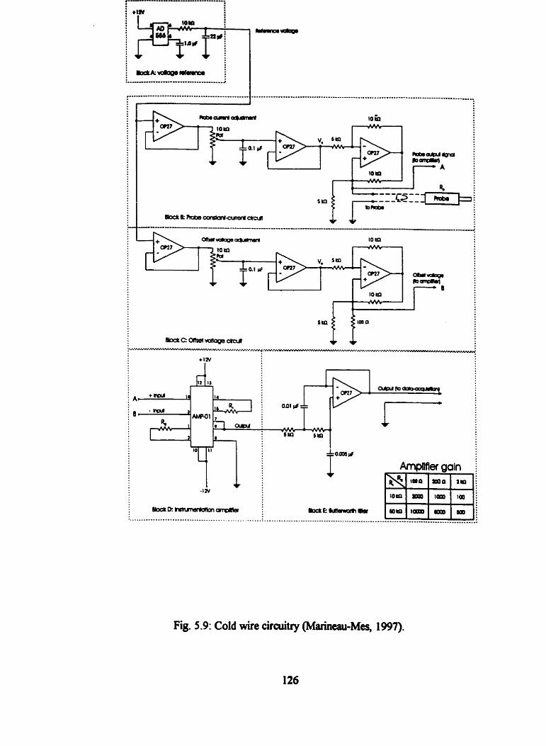
Fig. 5.9: Cold wire circuitry eau-Mes, 1997).

Fig. 6.1 : Typical variation of hot w k resistance with temperatwe.

Fig. 6.2: Orientation of the cross-wins.

128

Fis. 6.3: Determination of the cross-wires angles.

Fig. 6.4: Typical calitbration aims of the cross-wircs n,=0.44; nfl.42.

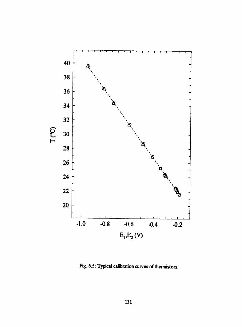
Fig. 6.6: Variations of cdd wire sensitivity with mean velocity.

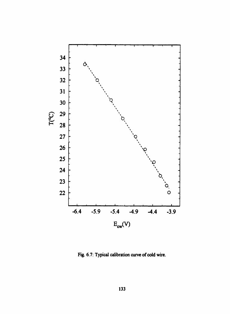
Fig. 6.7: Typical calibration aim of cdd wire.

Fig. 7.1 : Transverse profles of the mean velocity. Fuii symbois, Üc = 7.3 mls; empty

symbols, Ùc = 13.0 d s . 0 (shiAed by 0.3) and xJh = O; O (shifted by 0.4) rrid

x#= 6 (shüted by O. 1); A (shifted by 0.5) and A x/h = 1 1 (shiffed by 0.2).

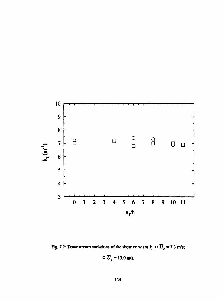
fig. 7.2: DoWllSfream variations of the shear constant k,. O Üc = 7.3 m/s;

0 Üc = 13.0 d s .

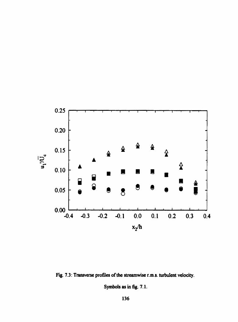
Fig 7.3 3: Transverse profiles of the streamwise r.m.s. turbulent velocity.

Symbols as in fig. 7.1.

136

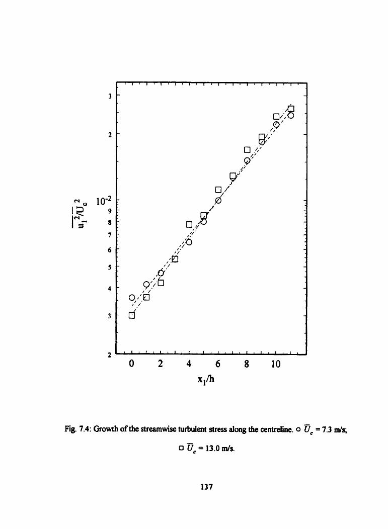
Fig. 7.4: Growth of the s t r e d s e turbulent stress dong the centrehe. O Üc = 7.3 mls;

0 Üc = 13.0 &S.

Fig. 7.5 : One-dimensiod normaüzed s m : . . . Re, = 172; - - - - ReA=311;

-- Re, = 476; - Re, = 578.

Fig. 7.6: Onedimensional normalued dissipation s-. . . . Re, = 172; - - - - Re, = 31 1;

-- Re, = 476; Re, = 578.

Fig. 7.7 : Variations of Kolmogorov's constant with ReAand r/q: . . . . ReA = 172; - - - Rr, = 31 1 (ShiAed by 0.5); -.-Re, = 476 (shifted by 1.0); ReA = 578 (shifted by 1.5). -

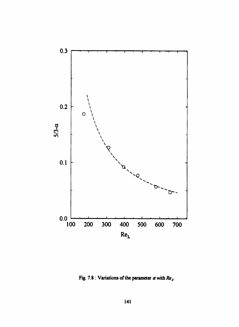
Fig. 7.8 : Variations of the pafameter awith Rr,.

141

Fig. 7.9: Corrected Koimogorov's constant: . . . Re, = 172 (shiAed by 1.5);

- - - - Re, = 3 11 (shiAd by 1); R e , = 476 (shified by 0.5); Ro, = 578. -

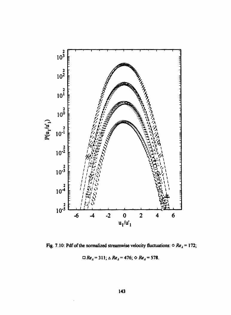
Fig. 7.10: Pdf of the normaüzed streamwise velocity fluctuations: 0 Re, = 172;

URo,=311;aReA=476;O Re,=S78.

Fig. 7.1 1 : Ratio of the variances of the velocity derivatives: 0 De = 7.3 d s ;

A Üe = 13 .O ds, fidi symbolq unco~ected.

Fig. 7.12: Pdf of the nomialid streamwise velocity denvative: 0 Re, = 172;

ReA = 31 1; A Re, = 476; v Re, = 578.

Fig. 7.13: Slope of the tails of the streamwise velocity derivative pdf : 0 positive ta&;

negative tails.

Fig. 7.14: Third moment of the pdf of the streamwir velocity derivative: - Re, = 172;

-- Re, = 3 1 1; - Re, = 476; - * = m g - Re, = 578.

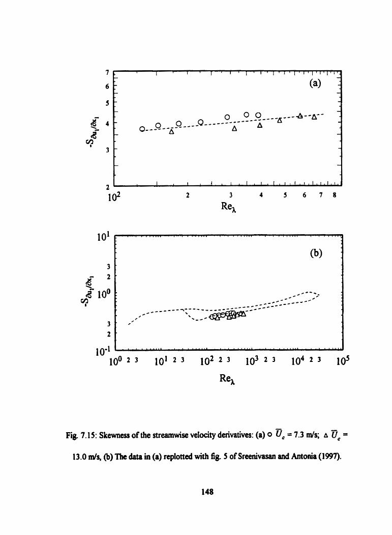
Fie. 7.15: Skewnesr of the strmwise velocity derivatives: (a) 0 Ûc = 7.3 mls; A Ûc =

13.0 ds, @) The data in (a) replotted with fig. 5 of Sreenivasan aMI Antonia (1997).

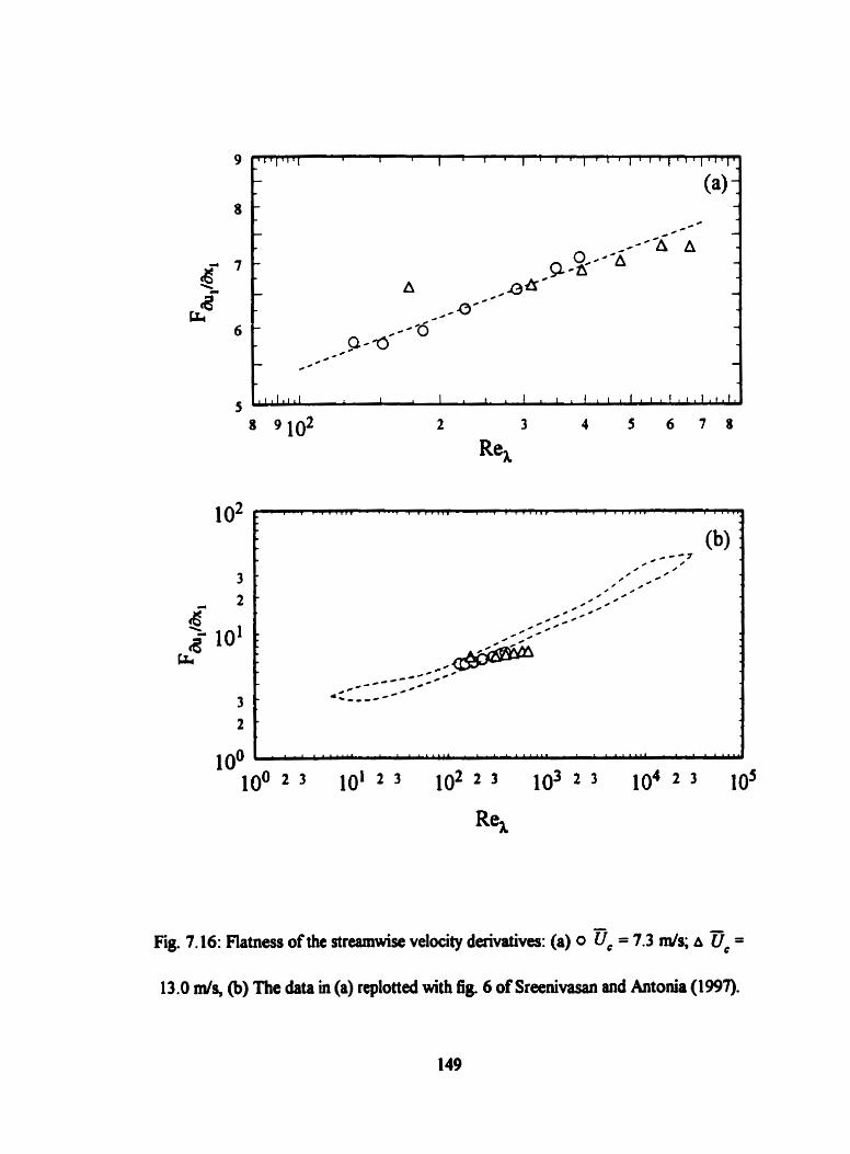
Fig 7.16: Fiatness of the streamwise velocity daivatives: (a) 0 = 7.3 d s ; A Üc =

13.0 mis, @) The data in (a) replotted with fig. 6 of Sreenivasan and Antonia (1997).

Fig 7.17: Pdf of the n o m a i i d transvase velocity derivative: 0 Re, = 172; O Re, = 3 1 1;

A Re, = 476; v Re, = 578.

Fig. 7.1 8: Slope of tails of the transverse velocity derivative pdf : 0 positive tails;

negative tails.

Fig. 7.19: Thkd moment of the pdf of the transverse velocity derivative: - Re, = 172;

-- Re, = 3 1 1; - Re, = 476; eme*-o Re, = 578.

Fig. 7.20: Skewness of the transverse velocity derivatives: 0 üc= 7.3 d s ; a Üc= 13 .O mis;

Tavoularis and Cornin (198 1 b); - Garg and WarhaA (1 998); . . . .. Pumir (1 9%).

Fig. 7.21: Flatness of the transverse velocity derivatives: 0 Üe= 7.3 ds; A De= 13.0 m/s;

Tavoukns and Comin (1981 b); 4 Garg and Wsmaft (1998).

Fig. 7.22: Pdf of the nonnalized strearnwise velocity diaerences at Re, = 578: 0 r/v = 2 1 ;

O r / l l = 76; A r/q = 142; v r/q = 210.

Fig. 7.23: Pdf of the normalizeû transverse velocity Merences at Re, = 578: O r/q= 2 1;

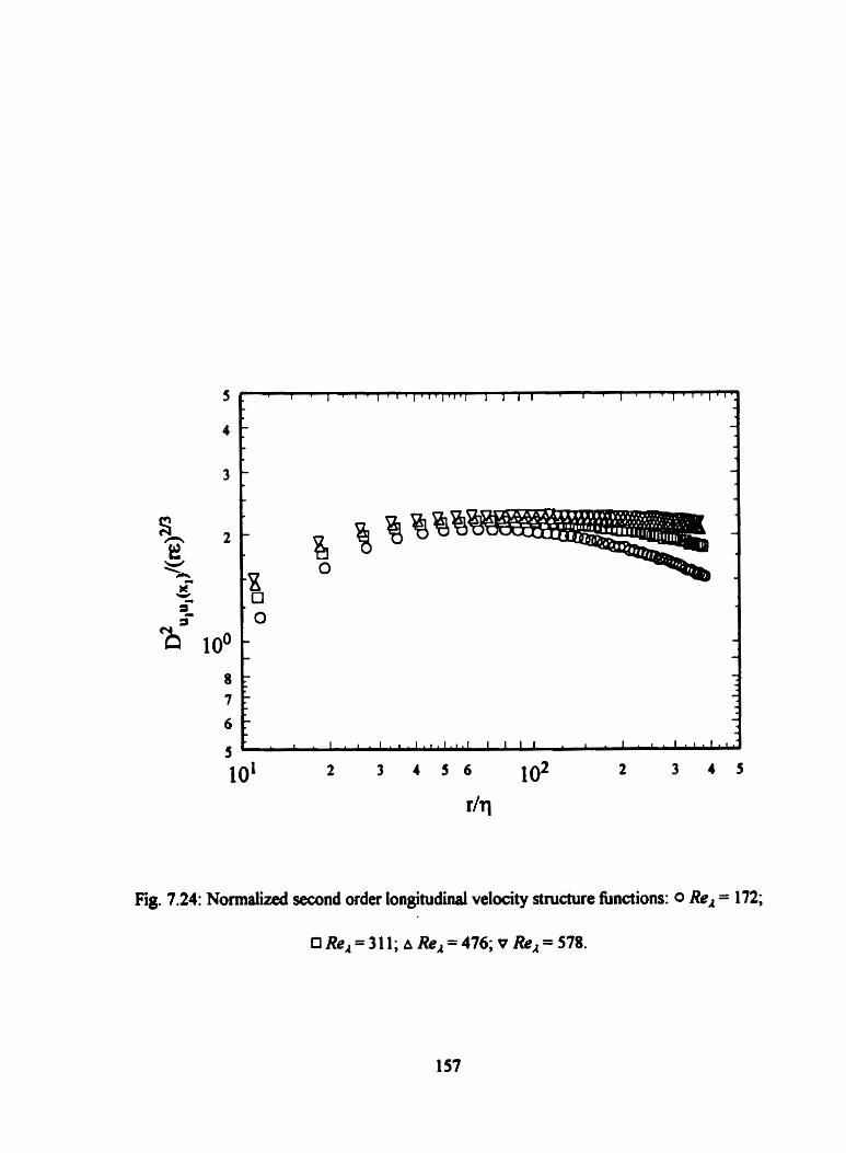
Fig. 7.24: NormalilPA second order longitudinal velocity structure functions: 0 Re, = 172;

ORe,=3 l l ; A ReA=476; v Re,=578.

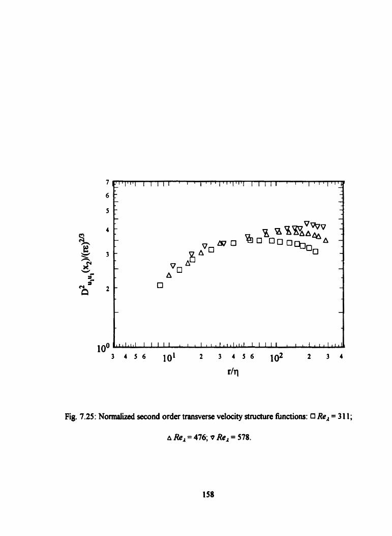
Fig. 7.25: N o d u e d second order transverse velocity structure functions: O Re, = 3 11;

A Re, = 476; v Re, = 578.

Fig. 7.26: Normaüzed third order longitudinal velocity structure fiinctions: 0 Re, = 172;

O Re, = 3 11; A Re, = 476; vRe, = 578.

Fig. 7.27: Skewness of the longitudinal velocity ciifference: 0 Re, = 172; O Re,= 3 1 1;

A ReA = 476; v Re, = 578.

Fig. 7.28: Normalized third order transverse velocity dEerence: 0 Re, = 3 1 1;

A Re, = 476; v Re, = 578.

Fig. 7.29: Skemess of the transverse velocity difference: 0 Re, = 172; O Re, = 3 1 1;

A Re, = 476; v ReA = 578. Fu1 symbols, measured with the h e d paraiiel hot wires.

Fig. 7.30: Fîatness of the longitudinal velocity daerence: 0 Re, = 172; 0 Re, = 3 1 1;

A Re, = 476; v Re, = 578.

Fig. 7.3 1 : Flatness of the transverse velocity daerence: 0 ReA = 1 72; O Re, = 3 1 1 ;

A Re, = 476; v Re, = 578. Full syrnbds, measured with the dxed paralle1 hot wires.

Fig. 7.32: Variations of the fiatness of the longitudinal velocity difference with r /q

Wq= 10; O r/q=20; A r/q=80; vr/q= 120; O r/q= 180.

165

Fis. 7.33: Variations of the flatness of the transverse velocity difference with r / q

W q = 1 O; iï r/q=20; A r/q=80; vr/q= 120; O r/q= 180.

166

". 1 ' 1 ' 1 ' , ' 1 ' 1 ' " 1 " ' 1 T 1 1 ' ' ' f ' 1 ' I ' l ' ~ " ' - - - - -

- -

O O 0 0 -

i O -

C

C 3 - -

- - - - - - -

-

- t

- h A A A A

P e v v V P -

_ O - d - - - - - - - - -

-

- C O 0 O 0 0 0 0 - - O L - - - - - - C

- w - O -

C - i 1 . 1 . 1 * l . i . l . l . l . 1 . l 1 I I I . t . I . i . l . l . l . l . l

Fig. 7.34: ~ormalized # order longitudinal structure fiinctions: op=2; O p=3; A p=4;

op=% Op=6.

Fig. 7.35:

Fig. 7.36: Corrected pd order longitudid structure fiinctions: op=2; Op=3; A p=4;

v p=5; O p=6.

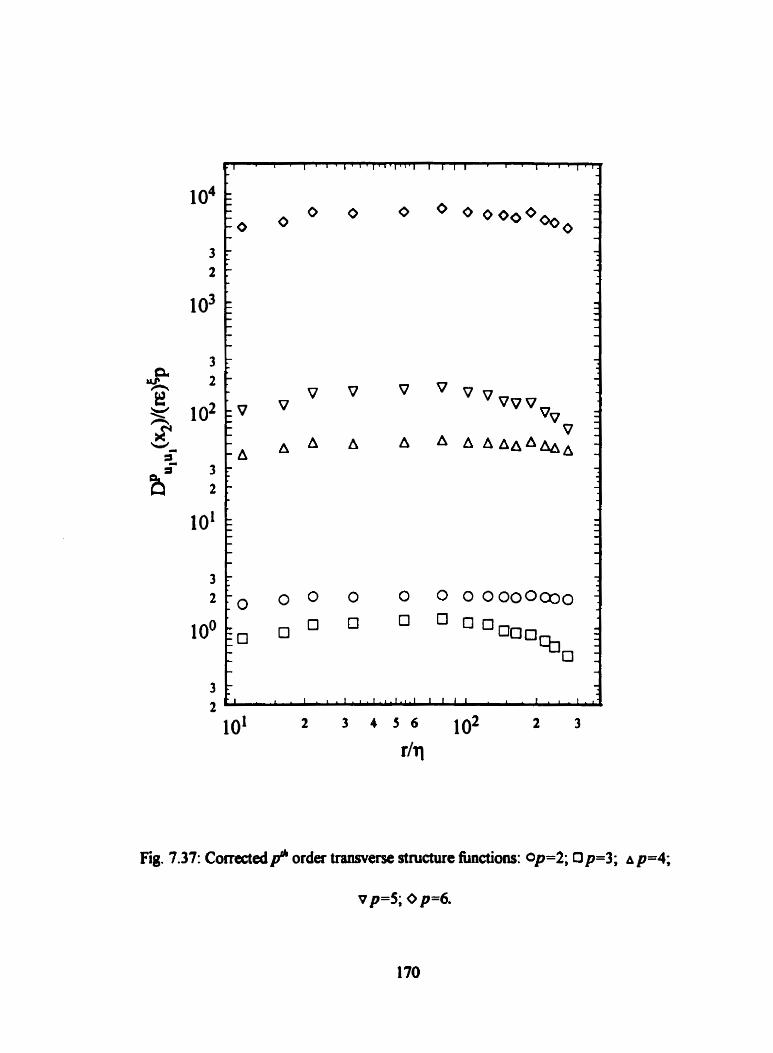
Fig. 7.37: Corrected order transverse structure fùnctions: op=2; O p=3; A p=4;

vp=5; Op=6.

O 1 2 3 4 5 6 7 8 9 1 0

P Fig. 7.38: Intennittency exponent variations with stnicture finction order: 0 detecminsd

form the longitudinal structure fiindion; O daermined fom the transverse structure

hction; A Anselmet et d. (1984); v Boratav (1997); - She and Lévêque (1994);

- (, = pl3 (Kolmogorov, 194 1).

Fig. 8.1 : Transverse profiles of the mean velocity in the heated fiow.

0 ~,/h=3; 0 ~JhC4.7; A x-.

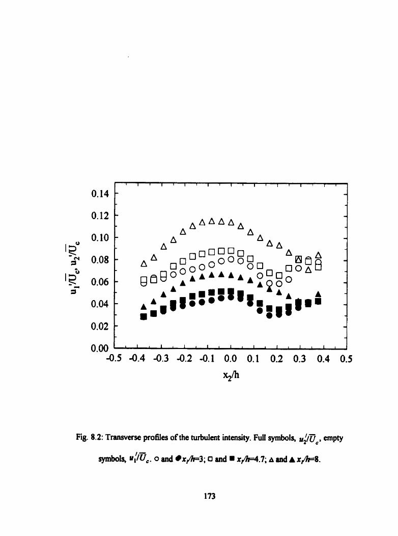
Fig. 8.2: Tramverse profiles of the turbulent intensity. Fd symbols, u $ ~ c , empty

symbols, u#üC. 0 and xJk3; a and xJhc4.7; a and A r e 8 .

Fig. 8.3: Transverse profles of the turbulent shear stress coefficient. o rm3;

x m . 7 ; A xJIFS*

Fig. 8.4: Growth of the turbulent intensities. 0 q/T ; qr.

Fig. 8 3: Downstream development of the shear stress coefficient.

Fig. 8.6: Downstrm developrnent of the integrai length scales. 0 LI , , ; 0 LI,,.

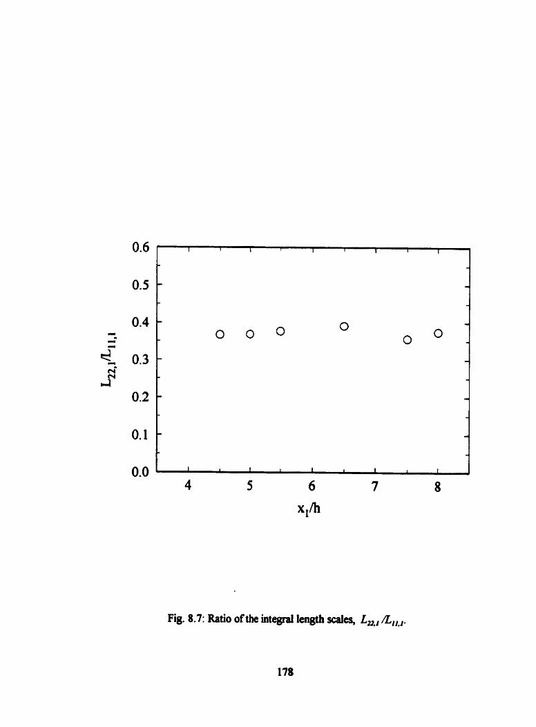
Fig. 8.7: Ratio of the integral length d e s , Ln,, a,,,.

Fig. 8.8: Pdf of the streamwise velocity fluctuations. 0 Re, = 184; CI Re, = 200;

A Re, = 253.

Fig. 8.9: Pdf of the transverse velocity fluctuations. 0 Re, = 184; O Re, = 200;

A Re, = 253.

Fig. 8.10: Transverse profiles of the mean temperature rise. 0 x+3; 0 x W . 7 ;

A xJIF8.

Fig. 8.1 1: Transverse profiles of the normalized temperature fluctuations. 0 x e 3 ;

O x W . 7 ; a x e 8 .

Fig. 8.12: Transverse profiies of the temperature-velocity correlatiom. Full

symbols, -PI@, empty symboh, h , e . 0 and x m ; O and . x W . 7 ; A and A x@8.

Fig. 8.13 : Growth of the normakâ temperature variance.

Fig. 8.14: Dowmtream development of the turbulent correlations. 0 pu CI -p%*. I

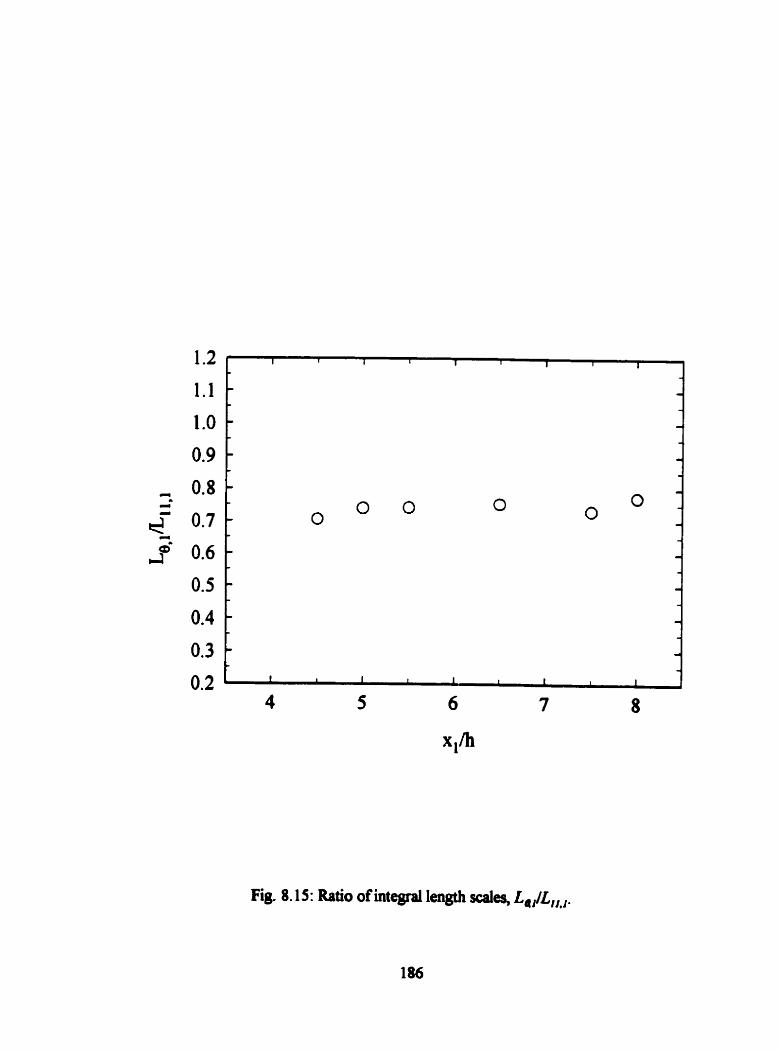
Fig. 8.1 5: Ratio of integral length d e s , L,&LIL,,.

Fig. 8.16: Pdf of the temperature fluctuations. 0 Re, = 184; 0 ReA = 200; A Re, = 253.

Fig. 8.17: Variations of skewness and fiatness of the temperohue fluctuations with Re,.

Fig. 8.18: Variations of the squared temperature-temperature dissipation correlation

coefficient with Re,.

Fig. 8.19: Nomialized co-spectra of the tempefatue-temperature dissipation.

- ReA = 2ûû; --- Re, = 253.

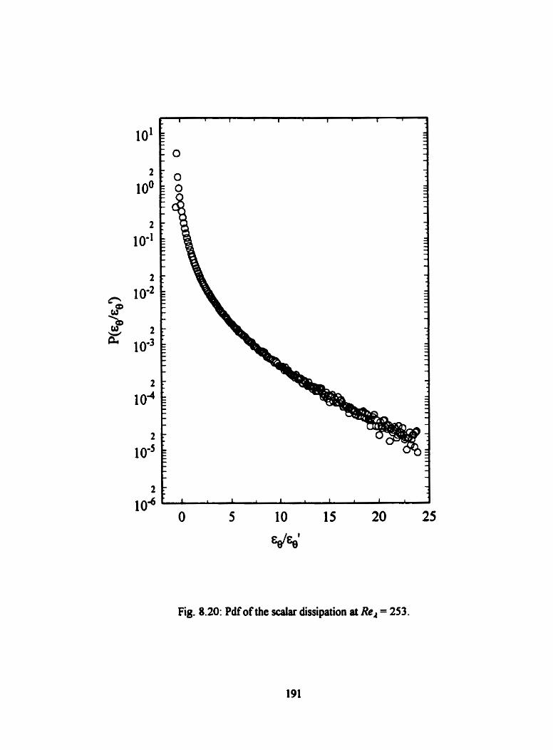
Fig. 8.20: Pdf of the scalar dissipation at Re, = 253.

Fig 8.22: Normaüzed conditionai expecbtion of the scalar dissipation.

0 Re, = 200; 0 ReA = 253.

Fig. 8.23 : Normalized conditionai expectation of the streamwise velocity fîuctuations.

0 Re,= 200; 0 Re,= 253.

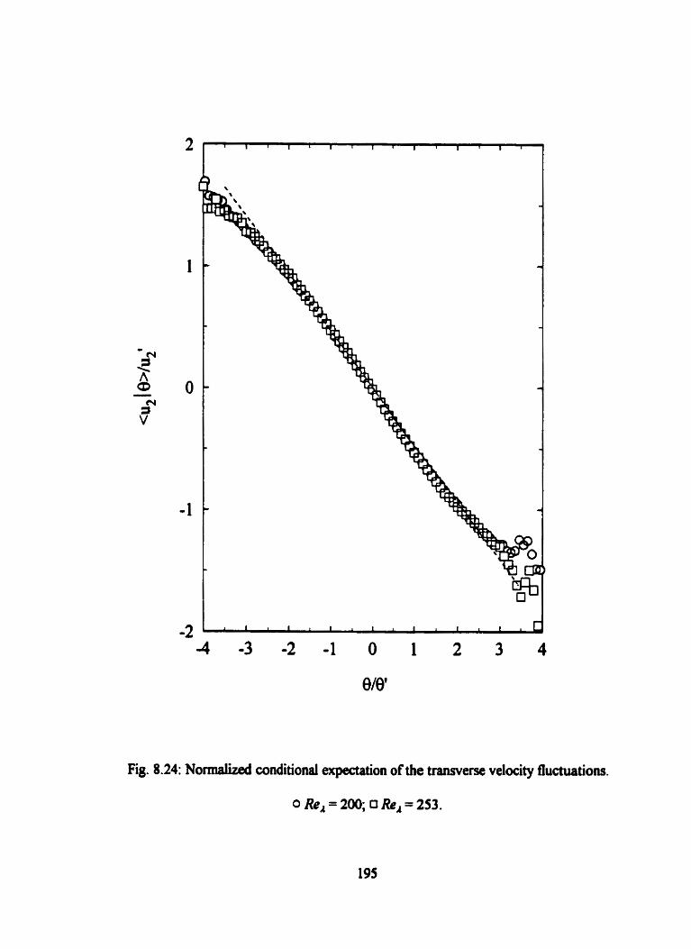
Fig. 8.24: NomialiLed conditional expectation of the transverse velocity fluctuations.

oRkp200, uRo,=253.

Fig. 8.25: th, iso-probabüity contours. - jointiy Gaussian;

0.15 ; 0.1--, ,0.01; . . -0.001.

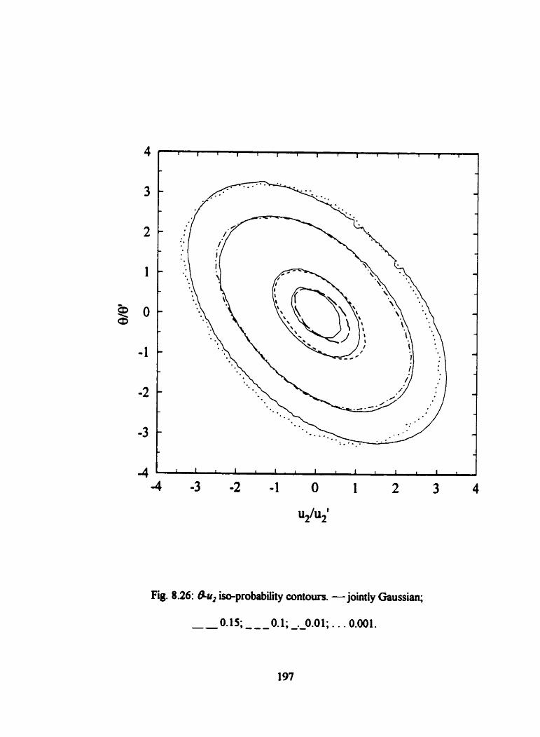
Fig. 8.26: au, iso-probabüity contours. - jointly Gaussian;

-- O. 15; --- 0.1; -.-0.01; . . .O.ool.

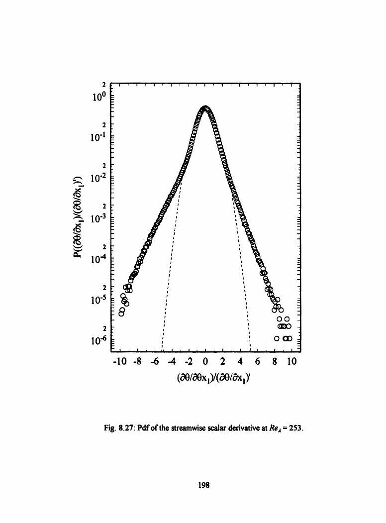
Fig. 8.27: Pdf of the strearnwise scalar derivative at Re, = 253.

Fig. 8.28: Pdf of the transverse scalar derivative at Re, = 200.

Fig. 8.29: Third moment of the pdf of the strmwise Scatar derivative at Re, = 200.

Fig. 8.30: Thkd moment of the @of the transverse scaiu derivative at ReA = 200.

Fig. 8.3 1 : (a) Variations of the skewness of the streamwise scaiar denvative wïtb Rr,

@) replotted with fig. 7 of Sreenivasan and Antonia (1997).

Fig. 8.32: (a) Variations of the flatness of the streamwise scalar derivative with Roi

(ô) replotted with fie. 8 Sreenivasan and Antonia (1997).

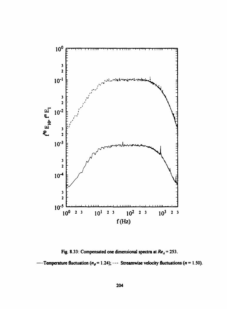
Fig. 8.33: Compensated one dimensional speara at Rr, = 253.

Temperatwc fluctuation (n, = 1 .M); --- Streamwise velocity fluctuations (n = 1 50).

Fig. 8.34: Pdf of the streamwise scalar difference at Re, = 253.

O r/q = 20; 0 r/q = 40; A r/q = 60; v r/q = 100.

Fig. 8.35: Pdf of the tranmerse scaiar Merence at Re, = 200.

O r/q = 26; 0 r/q = 37; A r/q = 79; v r/q = 156.

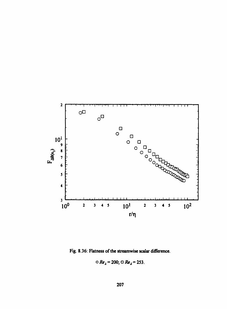
Fig. 8.36: Fiatness of the streamwise scalar difrenct.

0 Re, = 200; 0 ReA = 253.

Fig. 8.37: Flatness of the transverse scaiar difference at Re, = 200.

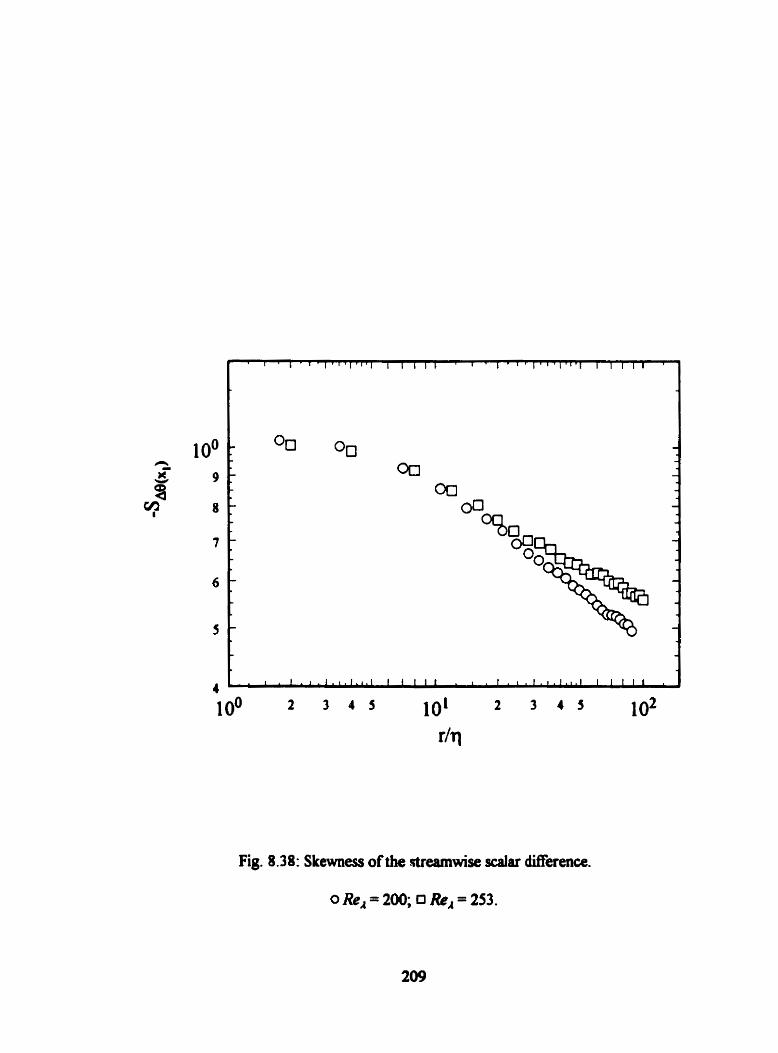
Fig. 8.38: Skemess of the ~eamwise scalar clifference.

0Re,=200;~1Rc,=253 .

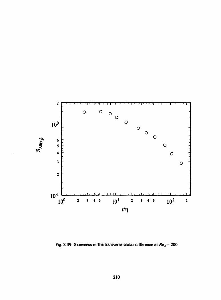
Fig. 8.39: Skewness of the transverse scelar clifference at Re, = 200.

APPENDM A

Mathematical Derivations

This appendix includes the denvations of equation 4.24 starting from equation 4.23

of Chapter 4.

1. The f h t tenn oa the right hand side of equation 4.23 cm be written as

therefore

II. aTla~, in the seçond term on the nght hand side of equation 4.23 can be taken out

of the average as

Using the produre developed in equation 3.40, -,il* b(0-$)> can be expressed

89

the last quation can be acpanded as

212

the first tenn in the above equation is zero, thereforq

where ~jû=$> is the conditional expectation of the velocity fluctuations conditional upon

the scalar 8.

III. The third term on the right hand side of equation 4.23 can be expanded as

a air. = --<u,b(e-~i)> + cL&(e-~rp

4 a

ar, = - -<~,b(e -$)>

4

the second and last steps followed fkom continuity, oL/o, = O. Again, anploying the

procedure of equation 3.40, CU, b(0-$)> can be expressed as

IV. The forth te- in a straightforward manner, gives

V. The last tenn on the right hand side of equation 4.23 is expandeci as

the second term of the above equation will be reduced as foliows

the above step foliows because 8 and 9 are independent. Expressing <y(bû/&j)2 b(0-1#)> in

tams of r conditional expectation by employing the procedure of quation 3.40, one gets

the last term on the right hand side of equation 4.23 therefore, reduces to

F i d y substituthg for ail the ternis on the nght hand side of equation 4.23 yields