leveraging 35 years of pinus taeda research in the...

Biogeosciences, 14, 3525–3547, 2017https://doi.org/10.5194/bg-14-3525-2017© Author(s) 2017. This work is distributed underthe Creative Commons Attribution 3.0 License.

Leveraging 35 years of Pinus taeda research in the southeastern USto constrain forest carbon cycle predictions: regional dataassimilation using ecosystem experimentsR. Quinn Thomas1, Evan B. Brooks1, Annika L. Jersild1, Eric J. Ward2, Randolph H. Wynne1, Timothy J. Albaugh1,Heather Dinon-Aldridge3, Harold E. Burkhart1, Jean-Christophe Domec4,5, Thomas R. Fox1,Carlos A. Gonzalez-Benecke6, Timothy A. Martin7, Asko Noormets8,a, David A. Sampson9, and Robert O. Teskey10

1Department of Forest Resources and Environmental Conservation, Virginia Tech, Blacksburg, VA, USA2Climate Change Science Institute and Environmental Sciences Division, Oak Ridge National Laboratory, Oak Ridge, TN,USA3State Climate Office of North Carolina, North Carolina State University, Raleigh, NC, USA4Bordeaux Sciences Agro, UMR 1391 INRA-ISPA, Gradignan CEDEX, France5Nicholas School of the Environment, Duke University, Durham, NC, USA6Department of Forest Engineering, Resources and Management, Oregon State University, Corvallis, OR, USA7School of Forest Resources and Conservation, University of Florida, Gainesville, FL, USA8Department of Forestry and Environmental Resources, North Carolina State University, Raleigh, NC, USA9Decision Center for a Desert City, Arizona State University, Tempe, AZ, USA10Warnell School of Forestry and Natural Resources, University of Georgia, Athens, Athens, GA, USAacurrent address: Department of Ecosystem Science and Management, Texas A&M University, College Station, TX, USA

Correspondence to: R. Quinn Thomas ([email protected])

Received: 14 February 2017 – Discussion started: 16 February 2017Revised: 22 May 2017 – Accepted: 19 June 2017 – Published: 26 July 2017

Abstract. Predicting how forest carbon cycling will changein response to climate change and management dependson the collective knowledge from measurements across en-vironmental gradients, ecosystem manipulations of globalchange factors, and mathematical models. Formally inte-grating these sources of knowledge through data assimila-tion, or model–data fusion, allows the use of past obser-vations to constrain model parameters and estimate predic-tion uncertainty. Data assimilation (DA) focused on the re-gional scale has the opportunity to integrate data from bothenvironmental gradients and experimental studies to con-strain model parameters. Here, we introduce a hierarchicalBayesian DA approach (Data Assimilation to Predict Produc-tivity for Ecosystems and Regions, DAPPER) that uses ob-servations of carbon stocks, carbon fluxes, water fluxes, andvegetation dynamics from loblolly pine plantation ecosys-tems across the southeastern US to constrain parameters ina modified version of the Physiological Principles Predict-

ing Growth (3-PG) forest growth model. The observations in-cluded major experiments that manipulated atmospheric car-bon dioxide (CO2) concentration, water, and nutrients, alongwith nonexperimental surveys that spanned environmentalgradients across an 8.6× 105 km2 region. We optimized re-gionally representative posterior distributions for model pa-rameters, which dependably predicted data from plots with-held from the data assimilation. While the mean bias in pre-dictions of nutrient fertilization experiments, irrigation ex-periments, and CO2 enrichment experiments was low, futurework needs to focus modifications to model structures thatdecrease the bias in predictions of drought experiments. Pre-dictions of how growth responded to elevated CO2 stronglydepended on whether ecosystem experiments were assimi-lated and whether the assimilated field plots in the CO2 studywere allowed to have different mortality parameters than theother field plots in the region. We present predictions of stembiomass productivity under elevated CO2, decreased precip-

Published by Copernicus Publications on behalf of the European Geosciences Union.

3526 R. Q. Thomas et al.: Leveraging 35 years of Pinus taeda research

itation, and increased nutrient availability that include esti-mates of uncertainty for the southeastern US. Overall, we(1) demonstrated how three decades of research in southeast-ern US planted pine forests can be used to develop DA tech-niques that use multiple locations, multiple data streams, andmultiple ecosystem experiment types to optimize parametersand (2) developed a tool for the development of future pre-dictions of forest productivity for natural resource managersthat leverage a rich dataset of integrated ecosystem observa-tions across a region.

1 Introduction

Forest ecosystems absorb and store a large fraction of an-thropogenic carbon dioxide (CO2) emissions (Le Quéré etal., 2015; Pan et al., 2011) and supply wood products to agrowing human population (Shvidenko et al., 2005). There-fore, predicting future carbon sequestration and timber sup-ply is critical for adapting forest management practices tofuture environmental conditions and for using forests to as-sist with the reduction in atmospheric CO2 concentrations.The key sources of information for developing these predic-tions are results from global change ecosystem manipulationexperiments, observations of forest dynamics across environ-mental gradients, and process-based ecosystem models. Thechallenge is integrating these three sources into a commonframework for creating probabilistic predictions that provideinformation on both the expected future state of the forestand the probability distribution of those future states.

Data assimilation (DA), or data–model fusion, is an in-creasingly used framework for integrating ecosystem obser-vations into ecosystem models (Luo et al., 2011; Niu et al.,2014; Williams et al., 2005). DA integrates observations withecosystem models through statistical, often Bayesian, meth-ods that can generate probability distributions for ecosys-tem model parameters and initial states. DA allows for theexplicit accounting of observational uncertainty (Keenan etal., 2011), the incorporation of multiple types of observa-tions with different timescales of collection (MacBean etal., 2016; Richardson et al., 2010), and the representation ofprior knowledge through informed parameter prior distribu-tions or specific relationships among parameters (Bloom andWilliams, 2015).

Using DA to parameterize ecosystem models with obser-vations from multiple locations that leverage ecosystem ma-nipulation experiments and environmental gradients will al-low for predictions to be consistent with the rich history ofglobal change research in forest ecosystems. Ecosystem ma-nipulation experiments provide a controlled environment inwhich data collected can be used to describe how forests ac-climate and operate under altered environmental conditions(Medlyn et al., 2015) and can potentially allow for the op-timization of model parameters associated with the altered

environmental factor in the experiment. Furthermore, the as-similation of data from ecosystem manipulation experimentsmay increase parameter identifiability (reducing equifinality;Luo et al., 2009), where two parameters have compensatingcontrols on the same processes, by isolating the response toa manipulated driver. Observations that span environmentalgradients include measures of forest ecosystem stocks andfluxes across a range of climatic conditions, nutrient avail-abilities, and soil water dynamics. These studies leveragetime and space to quantify the sensitivity of forest dynam-ics to environmental variation. However, covariation of en-vironmental variation can pose challenges separating the re-sponses to individual environmental factors. Overall, assimi-lating observations from a region that includes environmentalgradients and manipulation experiments is a useful extensionof prior DA research focused on DA at a single site with mul-tiple types of observations (Keenan et al., 2012; Richardsonet al., 2010; Weng and Luo, 2011).

Southeastern US planted pine forests are ideal ecosystemsfor exploring the application of DA to carbon cycle and for-est production predictions. These ecosystems are dominatedby loblolly pine (Pinus taeda L.), thus allowing for a singleparameter set to be applicable to a large region containingmany soil types and climatic gradients. Loblolly pine rep-resents more than one half of the standing pine volume inthe southern United States (11.7 million ha) and is by far thesingle most commercially important forest tree species forthe region, with more than 1 billion seedlings planted an-nually (Fox et al., 2007; McKeand et al., 2003). There isalso a rich history of experimental research located acrossthe region focused on global change factors that have in-cluded nutrient addition (Albaugh et al., 2016; Carlson et al.,2014; Raymond et al., 2016), water exclusion (Bartkowiaket al., 2015; Tang et al., 2004; Ward et al., 2015; Will etal., 2015), and water addition experiments (Albaugh et al.,2004; Allen et al., 2005; Samuelson et al., 2008). The re-gion also includes a multiyear ecosystem CO2 enrichmentstudy (McCarthy et al., 2010). Furthermore, many of theseexperiments are multi-factor with water exclusion by nutri-ent addition (Will et al., 2015), water addition by nutrientaddition (Albaugh et al., 2004; Allen et al., 2005; Samuelsonet al., 2008), and CO2 by nutrient addition treatments (Mc-Carthy et al., 2010; Oren et al., 2001). Beyond experimentaltreatments, southeastern US loblolly pine ecosystems includeat least two eddy-covariance sites with high-frequency mea-surements of C and water fluxes along with biometric ob-servations over many years (Noormets et al., 2010; Novicket al., 2015) and sites with multiyear sap flow data (Ewerset al., 2001; Gonzalez-Benecke and Martin, 2010; Phillipsand Oren, 2001). Finally, there are studies that include plotsthat span the regional environmental gradients and extendback to the 1980s (Burkhart et al., 1985). Overall, the multi-decadal availability of observations of C stocks (or biomass),leaf area index (LAI), C fluxes, water fluxes, and vegetationdynamics in plots with experimental manipulation and plots

Biogeosciences, 14, 3525–3547, 2017 www.biogeosciences.net/14/3525/2017/

R. Q. Thomas et al.: Leveraging 35 years of Pinus taeda research 3527

across environmental gradients, is well suited to potentiallyconstrain model parameters and predictions of how carboncycling responds to environmental change.

Using loblolly pine plantations across the southeastern USas a focal application, our objectives were to (1) developand evaluate a new DA approach that integrates diverse datafrom multiple locations and experimental treatments with anecosystem model to estimate the probability distribution ofmodel parameters, (2) examine how the predictive capacityand optimized parameters differ between an assimilation ap-proach that only uses environmental gradients and an assim-ilation approach that uses both environmental gradients andecosystem manipulations, and (3) demonstrate the capacityof the DA approach to predict, with uncertainty, regional for-est dynamics by simulating how forest productivity respondsto drought, nutrient fertilization, and elevated atmosphericCO2 across the southeastern US.

2 Methods

2.1 Observations

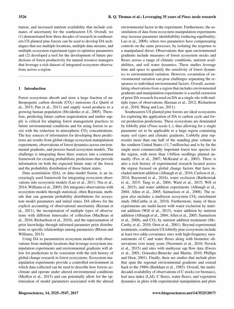
We used 13 different data streams from 294 plots at 187unique locations spread across the native range of loblollypine trees to constrain model parameters (Table 1; Fig. 1).The data streams covered the period between 1981 and 2015.The Forest Modeling Research Cooperative (FMRC) Thin-ning Study provides the largest number of plots that span theregion (Burkhart et al., 1985). In this study, we only used thecontrol plots that were not thinned. The Forest ProductivityCooperative (FPC) Region-wide 18 (RW18) study includedcontrol and nutrient fertilization addition plots that span theregion (134.4 kg ha−1 N + 13.44 kg ha−1 P biannually) (Al-baugh et al., 2015). The Pine Integrated Network: Educa-tion, Mitigation, and Adaptation Project (PINEMAP) studyincluded four locations dispersed across the region that in-cluded a replicated factorial experiment with control, nutrientfertilization (224 kg ha−1 N+ 27 kg ha−1 P+micronutrientsonce at project initiation), throughfall reduction (30 % reduc-tion), and fertilization by throughfall treatments (Will et al.,2015). The Southeast Tree Research and Education Site (SE-TRES) study was located at a single location and includedreplicated control, irrigation (∼ 650 mm of added water peryear), nutrient fertilization (∼ 100 kg N ha−1

+ 17 kg P ha−1

with micronutrients applied annually with absolute amountdepending on foliar nutrient ratios), and fertilization by irri-gation treatments (Albaugh et al., 2004). The Waycross studywas a single site with a non-replicated fertilization treatment.The annual application of nutrient fertilization was focusedon satisfying the nutrient demand by the trees and resultedin one of the most productive stands in the region (Bryars etal., 2013). These five studies included data streams of standstem biomass (defined as the sum of stem wood, stem bark,and branches) and live stem density. Waycross and SETRES

included LAI measurements from litterfall traps (Waycross)or estimates from LI-COR LAI-2000 (SETRES). SETRESalso included fine root and coarse root measurements. In thePINEMAP, SETRES, and RW18 studies we only used fo-liage biomass estimates from the control plots. We excludedthe foliage biomass estimates from the treatment plots be-cause they were derived from allometric models that may nothave captured changes in allometry due to the experimentaltreatment. We did use LAI measurements from both controland treatment plots where available (SETRES).

We also included observations from the Duke Free-AirCarbon Enrichment (FACE) study where the atmosphericCO2 was increased by 200 ppm above ambient concentra-tions. Based on the data presented in McCarthy et al. (2010),the study included six control plots, four CO2 fumigatedrings (including the unfertilized half of the prototype), twonitrogen fertilization treatments (115 kg N ha−1 yr−1 appliedannually), and one CO2 by nitrogen addition treatment (fer-tilized half of prototype). The Duke FACE study includedobservations of stem biomass (loblolly pine and hardwood),coarse root biomass (loblolly pine and hardwood), fine rootbiomass (combined loblolly pine and hardwood), stem den-sity (loblolly pine only), leaf turnover (combined loblollypine and hardwood), fine root production (combined loblollypine and hardwood), and monthly LAI (loblolly pine andhardwood).

Finally, we included two AmeriFlux sites with eddy-covariance towers in loblolly pine stands. The US-DK3 sitewas located in the same forest as the Duke FACE site de-scribed above (Novick et al., 2015). The US-NC2 site waslocated in coastal North Carolina (Noormets et al., 2010). Weused monthly gross ecosystem production (GEP; modeledgross primary productivity from net ecosystem exchangemeasured at an eddy-covariance tower) and evapotranspira-tion (ET) estimates from the sites. The monthly GEP and ETwere gap-filled by the site principal investigator. The GEPwas a flux-partitioned product created by the site principalinvestigator. The biometric data from the US-DK3 site wereassumed to be the same as the first control ring. The biomet-ric data from the US-NC2 site included observations of stembiomass (loblolly pine and hardwood), coarse root biomass(loblolly pine and hardwood), fine root biomass (combinedloblolly pine and hardwood), stem density (loblolly pineonly), leaf turnover (combined loblolly pine and hardwood),and fine root production (combined loblolly pine and hard-wood).

2.2 Ecosystem model

We used a modified version of the Physiological PrinciplesPredicting Growth (3-PG) model to simulate vegetation dy-namics in loblolly pine stands (Bryars et al., 2013; Gonzalez-Benecke et al., 2016; Landsberg and Waring, 1997). 3-PG is astand-level vegetation model that runs at a monthly time stepand includes vegetation carbon dynamics and a simple soil

www.biogeosciences.net/14/3525/2017/ Biogeosciences, 14, 3525–3547, 2017


Table 1. Regional observational data streams used in data assimilation.

Data stream Measurement Measurement Uncertainty Streamfrequency or estimation ID for

technique Table 3

Foliage biomass (Pine) Annual or less Allometric relationship Based on propagating the al-lometric model uncertainty inGonzalez-Benecke et al. (2014).Varied by observation.

1

Foliage biomass(hardwood)

Annual or less Allometric relationship Assumed zero 2

Stem biomass (pine) Annual or less Allometric relationship Based on propagating theallometric model uncertaintyin Gonzalez-Benecke et al.(2014).Varied by observation.

3

Stem biomass(hardwood)

Annual or less Allometric relationship Assumed zero 4

Coarse root biomass(combined)

Annual or less Allometric relationship Assumed zero∗ 5

Fine root biomass(combined)

Annual or less Allometric relationship SD: 10 % of observation 6

Foliage biomassproduction (combined)

Annual Litterfall traps SD: 10 % of observation 7

Fine root biomassproduction (combined)

Annual Mini-rhizotrons SD: 10 % of observation 8

Pine stem density Annual or less Counting individuals 1% (assumed small) 9

Leaf area index (pine) Monthly toannual

Litter traps or LI 2000 SD: 10 % of observation 10

Leaf area index(hardwood)

Monthly toannual


Leaf area index(combined)

Only used ifnot separatedinto pine andhardwood


Gross ecosystemproduction

Monthly Modeled from fluxeddy-covariance netecosystem exchange

SD: 10 % of observation 13

Evapotranspiration Monthly Eddy covariance SD: 10 % of observation 14

∗ The relatively low number of observations prevented convergence when using the observational uncertainty model, so observational uncertainty was assumed tobe zero to allow convergence.

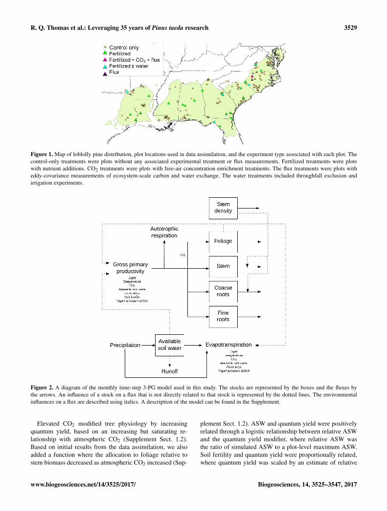
water bucket model (Fig. 2). While a complete description ofthe 3-PG model and our modifications can be found in theSupplement Sect. 1, the key concept for interpreting the re-sults is that gross primary productivity (GPP) was simulatedusing a light-use efficiency approach where the absorbedphotosynthetically active radiation (APAR) was converted tocarbon based on a quantum yield (Supplement Sect. 1.1).Quantum yield was simulated using a parameterized maxi-

mum quantum yield (alpha) that was modified by environ-mental conditions including atmospheric CO2, available soilwater (ASW), and soil fertility (Supplement Sect. 1.2–1.3).The ASW and soil fertility modifiers were values between 0and 1, while the atmospheric CO2 modifier had a value of 1at 350 ppm (thus values greater than 1 at higher CO2 concen-trations).



Figure 1. Map of loblolly pine distribution, plot locations used in data assimilation, and the experiment type associated with each plot. Thecontrol-only treatments were plots without any associated experimental treatment or flux measurements. Fertilized treatments were plotswith nutrient additions. CO2 treatments were plots with free-air concentration enrichment treatments. The flux treatments were plots witheddy-covariance measurements of ecosystem-scale carbon and water exchange. The water treatments included throughfall exclusion andirrigation experiments.

Figure 2. A diagram of the monthly time-step 3-PG model used in this study. The stocks are represented by the boxes and the fluxes bythe arrows. An influence of a stock on a flux that is not directly related to that stock is represented by the dotted lines. The environmentalinfluences on a flux are described using italics. A description of the model can be found in the Supplement.

Elevated CO2 modified tree physiology by increasingquantum yield, based on an increasing but saturating re-lationship with atmospheric CO2 (Supplement Sect. 1.2).Based on initial results from the data assimilation, we alsoadded a function where the allocation to foliage relative tostem biomass decreased as atmospheric CO2 increased (Sup-

plement Sect. 1.2). ASW and quantum yield were positivelyrelated through a logistic relationship between relative ASWand the quantum yield modifier, where relative ASW wasthe ratio of simulated ASW to a plot-level maximum ASW.Soil fertility and quantum yield were proportionally related,where quantum yield was scaled by an estimate of relative



stand-level fertility (a value of 1 was the maximum fertility).The fertility modifier (or soil fertility rating, FR) was con-stant throughout a simulation of a plot and was either basedon site characteristics or directly optimized as a stand-levelparameter (Supplement Sect. 1.3). For plots with nutrient fer-tilization, FR was a directly optimized parameter or set to 1,depending on the level of fertilization (see below). For un-fertilized plots, we used site index (SI), a measure of theheight of a stand at a specified age (25 years), to estimate FR.This approach is in keeping with previous efforts (Gonzalez-Benecke et al., 2016; Subedi et al., 2015); however, SI doesnot solely represent the nutrient availability of an ecosystem.For a given climate SI captures differences in soil fertility,where a lower SI corresponded to a site with lower fertility,but regional variation in SI also included the influence of cli-mate on growth rates that were already accounted for in theother environmental modifiers in the 3-PG model. When aclimate term is not used in the empirical FR model, FR is rel-ative to the highest SI in the region, which does not occur inthe northern extent of the region even in fertilized plots dueto climatic constraints. Thus, we also included the histori-cal (1970–2011) 35-year mean annual temperature (MAT) asan additional predictor, resulting in an empirical relationshipthat predicted FR as an increasing, but saturating, functionof SI within areas of similar long-term temperature. For ourapplication of the 3-PG model using DA, we removed thepreviously simulated dependence of total root allocation onFR (Bryars et al., 2013; Gonzalez-Benecke et al., 2016) be-cause we separated coarse and fine roots. Other environmen-tal conditions influenced GPP, including temperature, frostdays, and vapor pressure deficit (VPD). A description ofthese modifiers can be found in Supplement Sect. 1.2.

Each month, net primary production (a parameterized andconstant proportion of GPP) was allocated to foliage, stem(stem wood, stem bark, and branches), coarse roots, and fineroots (Supplement Sect. 1.4). Differing from previous ap-plications of 3-PG to loblolly pine ecosystems, we modi-fied the model to simulate fine roots and coarse roots sep-arately. 3-PG also simulated simple population dynamics byincluding stem density as a state variable. Stem density andstem biomass pools were reduced by both density-dependentmortality, based on the concept of self-thinning (Landsbergand Waring, 1997), and density-independent mortality, a newmodification where a constant proportion of individuals dieeach month (Supplement Sect. 1.5). Finally, we added asimple model of hardwood understory vegetation to enablethe assimilation of GEP and ET observations from eddy-covariance tower studies with significant understories (Sup-plement Sect. 1.7).

The water cycle was a simple bucket model with transpi-ration predicted using a Penman–Monteith approach (Bryarset al., 2013; Gonzalez-Benecke et al., 2016; Landsberg andWaring, 1997) (Supplement Sect. 1.6). The canopy conduc-tance used in the Penman–Monteith subroutine was modi-fied by environmental conditions. The modifiers included the

same ASW and VPD modifier as used in the GPP calcula-tion. Maximum canopy conductance occurred when simu-lated LAI exceeded a parameterized value of LAI (LAIgcx).Evaporation was equal to the precipitation intercepted by thecanopy. Runoff occurred when the ASW exceeded a plot-specific maximum ASW. As in prior applications of 3-PG,ASW was not allowed to take a value below a minimumASW, resulting in an implicit irrigation in very dry condi-tions. This assumption may cause the model to be less sen-sitive to low ASW, but the optimized parameterization maycompensate for this.

The 3-PG model used in this study simulated the monthlychange in 11 state variables per plot: four stocks for loblollypines, five stocks for understory hardwoods, loblolly pinestem density (stems ha−1), and ASW. The key fluxes thatwere used for DA included monthly GEP, monthly ET, an-nual root turnover, and annual foliage turnover. In total, 46parameters were required by 3-PG. The model required meandaily maximum temperature, mean daily minimum tempera-ture, mean daily PAR, total frost days per month, total rainper month, annual atmospheric CO2, and latitude. Each plotalso required maximum ASW, SI, MAT, and the initial con-dition of the 11 state variables as model inputs (Fig. 3).

We used the first observation at the plot as the initial condi-tions for the loblolly pine vegetation states (foliage biomass,stem biomass, coarse root biomass, fine root biomass, andstem number). When observations of coarse biomass and fineroot biomass were not available, these stocks were initial-ized as a mean region-wide proportion of the observed stembiomass. However, the value of initial root biomass in plotswithout observations was not important because root biomassdid not influence any other functions in the model. The hard-wood understory stocks at US-DK3 and US-NC2 were alsoinitialized using the first set of observations. Initial fine rootand coarse biomass were distributed between loblolly pineand hardwoods based on their relative contribution of totalinitial foliage biomass. The initialized ASW was assumedto be equal to the maximum ASW because most plots wereinitialized in winter months when plant demand for waterwas minimal. The maximum ASW in each plot was extractedfrom the Soil Survey Geographic Database (SSURGO) soilsdataset (Soil Survey Staff, 2013). The value we used corre-sponded to the maximum ASW for the top 1.5 m of the soil.We assumed that the minimum ASW was zero. Because wefocused on a region-wide optimization, we used region-wide4 km estimates of observed monthly meteorology as inputsand to calculate the 35-year MAT for each plot (Abatzoglou,2013). SI was based on height measurements at age 25 ineach plot or calculated by combining observations of heightat younger ages with an empirical model (Dieguez-Aranda etal., 2006).

We simulated ecosystem manipulation experiments in the3-PG model by altering the environmental modifiers or bymodifying the environmental inputs. Nutrient addition exper-iments were simulated by setting FR equal to 1 for the studies



Figure 3. Key climatic and stand characteristic inputs to the regional 3-PG simulations: (a) mean annual temperature (1979–2011) as asummary of the gradient in monthly temperature inputs used in simulations, (b) maximum available soil water for the top 1.5 m of soil fromSSURGO, (c) mean annual precipitation (1979–2011) as a summary of the gradient in monthly precipitation inputs used in simulations, and(d) site index. The area shown is the natural range of loblolly pine (Pinus taeda L.).

that applied nutrients at regular intervals to remove nutrientdeficiencies (RW18, SETRES, Waycross). FR was directlyestimated for fertilized plots in two of the studies either be-cause nutrients were only added once at the beginning of thestudy (PINEMAP), thus potentially not removing nutrientlimitation, or because nitrogen was the only element added(Duke FACE), thus allowing the potential for nutrient limita-tion by other elements. For these plots, we also assumed thatthe FR of the fertilized plot was equal to or larger than thecontrol plot. Throughfall exclusion experiments were simu-lated by decreasing the throughfall by 30 % in the treatmentplots. The SETRES irrigation experiments were simulated byadding 650 mm to ASW between April and October. CO2enrichment experiments were simulated by setting the atmo-spheric CO2 input equal to the treatment mean from the el-evated CO2 rings (570 ppm). One plot (US-NC2) includeda thinning treatment during the period of observation. Wesimulated the thinning by specifying a decrease in the stemcount that matched the proportion removed at the site, withthe biomass of each tree equivalent to the average of trees inthe plot.

2.3 Data assimilation method

We used a hierarchical Bayesian framework to estimate theposterior distributions of parameters, latent states of stocksand fluxes, and process uncertainty parameters. The latentstates represented a value of the stock or flux before uncer-tainty was added through measurement. The approach was asfollows.

Consider a stock or flux (m) for a single plot (p) at time t(qp,m,t ). qp,m,t is influenced by the processes represented inthe 3-PG model and a normally distributed model processerror term,

qp,m,t ∼ N(f(θ ,FRp

),σm

), (1)

where θ is a vector of parameters that are optimized, FRp isthe site fertility, and σm is the model process error. Not shownare the vector of parameters that were not optimized (Supple-mental Table S1), the plot ASW, an array of climate inputs,and the initial conditions because these were assumed knownand not estimated in the hierarchical model. The process er-ror assumed that the error linearly scales with the magnitude



of the prediction:

σ 2m = γm+ ρmf

(θ ,FRp

). (2)

While the structure of the Bayesian model allowed for alldata streams to have process uncertainty that scales with theprediction, in this application we only allowed stem biomass,GEP, and ET process uncertainty to scale because they hadlarge variation across space (stem biomass) and through time(i.e., there should be lower process uncertainty in the winterwhen GEP is lower). For the other data streams, the linearscaling term was removed by fixing ρm at 0.

FRp did not have an explicit probability distribution.Rather the probability density was evaluated as 1 if the plotwas not fertilized, thus causing FRp to be estimated from SIand MAT (Supplement Eq. 15), or if it was a fertilized plotand had an FRp equal or higher than that of its non-fertilizedcontrol plot. The probability density was evaluated as 0 if theestimated FRp in a fertilized plot was less than the FRp inthe control plot or if FRp was not contained in the intervalbetween 0 and 1.

FRp ∼

1 if non-fertilized, FRp ≥ 0, and FRp ≤ 11 if FRp = 1 and fertilization levels are assumed toremove nutrient deficiencies0 if FRp < 1 and fertilization levels are assumed toremove nutrient deficiencies1 if fertilized but levels are not assumed to remove deficiencies andFRp ≥ FR of control plot0 if fertilized but levels are not assumed to remove deficiencies andFRp < FR of control plot0 if FRp < 0 or FRp > 1

(3)

Our model included the effect of observational errors formeasurements of stocks and fluxes. For a single stock or fluxfor a plot at time t there was an observation (yp,m,t ). Thenormally distributed observation error model was

yp,m,t ∼ N(qp,m,t ,τ2p,m,t ), (4)

where τ 2p,m,t represented the measurement error of the ob-

served state or flux. By including the observational errormodel, qp,m,t represented the latent, or unobserved, stock orflux. The variance was unique to each observation because itwas represented as a proportion of the observed value. Theτ 2p,m,t was assumed known (Table 1) and not estimated in the

hierarchical model.The hierarchical model required prior distributions for all

optimized parameters, including the parameters for the 3-PG model (θ ), FRp, and the process error parameters. Theprior distributions for (p(θ)) are specified in Table 3. Someparameters were informed by previous research in loblollypine ecosystems, while other parameters were “uninforma-tive” with flat distributions that had broad, but physically rea-sonable, bounds. The prior distributions for the process errorparameters were non-informative and had a uniform distribu-tion with upper and lower bounds that spanned the range of

reasonable error terms.

γm ∼ U (0.001,100) (5)ρm ∼ U(0,10) (6)

By combining the data, process, and prior models, our jointposterior that includes all 13 data streams, plots, months withobservations, and fitted parameters was

p(θ ,y,γ ,q|y,τ ,priors)∝,P∏p=1

M∏m=1

T∏t=1N(qp,m,t |f

(θ ,FRp

),γm+ ρmf

(θ ,FRp

)),

P∏p=1

M∏m=1

T∏t=1N(yp,m,t |qp,m,t ,τ

2p,m,t ), (7)

P∏p=1

p(FRp)

F∏f=1

p(θf )

M∏m=1

p(γm)

M∏m=1

p(ρm),

where bolded components represent vectors, P is the totalnumber of plots, M is the total number of data streams, T isthe total months with observations, and F is the total numberof 3-PG parameters that are optimized.

We numerically estimated the joint posterior distributionusing the Monte Carlo Markov Chain–Metropolis Hasting(MCMC-MH) algorithm (Zobitz et al., 2011). This approachhas been widely used to approximate parameter distributionsin ecosystem DA research (Fox et al., 2009; Trudinger etal., 2007; Williams et al., 2005; Zobitz et al., 2011). Briefly,the algorithm proposed new values for the model parameters,uncertainty parameters, latent states, and FR. The proposedvalues were generated using a random draw from a normaldistribution with a mean equal to the previously acceptedvalue for that parameter and standard deviation equal to theparameter-specific jumping size. The ratio of the proposedcalculation of Eq. (7) to the previously accepted calculationof Eq. (7) was used to determine if the proposed parameterwas accepted. If the ratio was greater than or equal to 1, theproposed value was always accepted. If the ratio was lessthan 1, a random number between 0 and 1 was drawn and theproposed value was accepted if the ratio was greater than therandom number. This allowed less probable parameter setsto be accepted, thus sampling the posterior distribution. Weadapted the size of the jump size for each parameter to en-sure the acceptance rate of the parameter set was between22 and 43 % (Ziehn et al., 2012) by adjusting the jump sizeif the acceptance rate for a parameter was outside the 22–43 % range. All MCMC-MH chains were run for 30 millioniterations with the first 15 million iterations discarded as theburn-in. Four chains were run and tested for convergence us-ing the Gelman–Rubin convergence criterion, where a valuefor the criterion less than 1.1 indicated an acceptable levelof convergence. We sampled every 1000th parameter in thefinal 15 million iterations of the MCMC-MH chain and usedthis thinned chain in the analysis described below. The 3-PG



model and MCMC-MH algorithm were programmed in For-tran 90 and used OpenMP to parallelize the simulation ofeach plot within an iteration of the MCMC-MH algorithm.

2.4 Data assimilation evaluation

Using the observations, model, and hierarchical Bayesianmethod described above, we assimilated both the non-manipulated and manipulated plots (Base assimilation; Ta-ble 4). We assessed model performance first by calculatingthe RMSE and bias of stem biomass predictions (the mostcommon data stream). In the evaluation, we only used themost recent observed values to increase the time length be-tween initialization and validation. Second, we assessed thepredictive capacity by comparing model predictions to datanot used in the parameter optimization in a cross-validationstudy. In this evaluation, we repeated the Base assimilationwithout 160 FMRC thinning study plots (Table 2), predictedthe 160 plots using the median parameter values, and calcu-lated the RMSE and bias stem biomass of the independentset of plots. Rather than holding out all 160 plots from a sin-gle assimilation and not generating a converged chain, wedivided the 160 plots into four unique sets of 40 plots andrepeated the assimilation for each set. Finally, we comparedthe predicted responses to experimental manipulation to theobserved responses. We focused the comparison on the per-centage difference in stem biomass between the control andtreatment plots. We used a paired t test to test for differencesbetween the predicted and observed responses within an ex-perimental type (irrigated, drought, nutrient addition, and el-evated CO2). We combined the single and multi-factor treat-ments for analysis. For the analysis of the nutrient additionstudies, we only used plots where FR was assumed to be 1 sothat we were able to simulate the treatments without requir-ing the optimization of a site-specific FR parameter.

During preliminary analysis, we found that the Base as-similation predicted lower stem biomass than observed inthe elevated CO2 plots in the Duke FACE study. Furtheranalysis investigating the cause of the bias in the CO2 plotsshowed that three parameters (wSx1000, ThinPower, andpCRS) were required to be unique to the Duke FACE studyin order to reduce the bias. Therefore, the Base assimilationincluded unique parameters for wSx1000, ThinPower, andpCRS parameters in all plots in the Duke FACE and US-DK3studies. To highlight the need for the site-specific parame-ters, we repeated the Base assimilation approach without thethree additional parameters for the Duke studies (NoDkParsassimilation).

2.5 Sensitivity to the inclusion of ecosystemexperiments

We also evaluated how parameter distributions and the as-sociated environmental sensitivity of model predictions de-pended on the inclusion of ecosystem experiments in data as-

similation. First, we repeated the Base assimilation, this timeexcluding the plots that included the manipulated treatments(NoExp). We removed all manipulation types at once, ratherthan individual experimental types, because all experimentaltypes involved multi-factor studies. The NoExp assimilationhad the same number of data streams as the Base assimi-lation because it included the control treatments from theexperimental studies. The NoExp assimilation representedthe situation where only observations across environmentalgradients were available. Second, we compared the param-eterization of the ASW, soil fertility, and atmospheric CO2environmental modifiers from the Base to the NoExp as-similation. The modifier equations are described in Supple-ment Sects. 1.2 and 1.3. Third, we repeated the same inde-pendent validation exercise for the 160 FMRC plots as de-scribed above for the Base assimilation. Fourth, we predictedthe treatment plots in the irrigated, drought, nutrient addition(only plots where FR was assumed to be 1), and elevatedCO2 plots. As for the Base assimilation, we used a t test tocompare the experimental response between the NoExp as-similation and observed values and between the NoExp andBase assimilations. Since the experimental treatments werenot used in the optimization, this was an independent evalu-ation of predictive capacity.

2.6 Regional predictions with uncertainty

To demonstrate the capacity of the data assimilation systemto create regional predictions with uncertainty, we simulatedthe regional response to a decrease in precipitation, an in-crease in nutrient availability, and an increase in atmosphericCO2 concentration, each as a single factor change from a1985–2011 baseline. Each prediction included uncertainty byintegrating across the parameter posterior distributions usinga Monte Carlo sample of the parameter chains. Our regioncorresponded to the native range of loblolly pine and usedthe HUC12 (USGS 12-digit Hydrological Unit Code) wa-tershed as the scale of simulation. For each HUC12 in theregion, we used the mean SI, 30-year mean annual tempera-ture, ASW aggregated to the HUC12 level, and monthly me-teorology from Abatzoglou (2013) as inputs (Fig. 3). The SIof each HUC12 was estimated from biophysical variablesin the HUC12 using the method described in Sabatia andBurkhart (2014). This SI corresponded to an estimated SI forstands without intensive silvicultural treatments or advancedgenetics of planted stock.

To sample parameter uncertainty, we randomly drew500 samples, with replacement, from the Base assimilationMCMC chain and simulated forest development from a 1985planting to age 25 in 2011 in each HUC. We chose age 25as the final age because it is a typical age of harvest in theregion. For each sample, we repeated the regional simula-tion with (1) a 30 % reduction in precipitation, (2) FR set to1, and (3) atmospheric CO2 increased by 200 ppm. Within aparameter sample, we calculated the percent change in stem



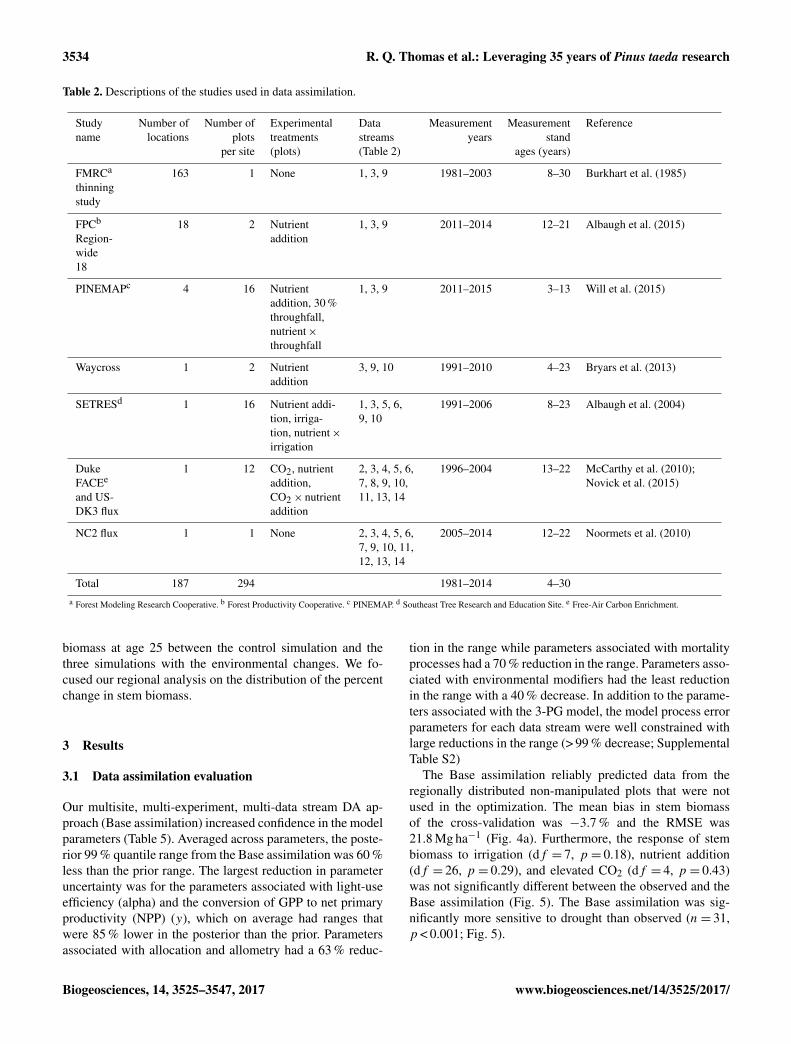
Table 2. Descriptions of the studies used in data assimilation.

Study Number of Number of Experimental Data Measurement Measurement Referencename locations plots treatments streams years stand

per site (plots) (Table 2) ages (years)

FMRCa

thinningstudy

163 1 None 1, 3, 9 1981–2003 8–30 Burkhart et al. (1985)

FPCb

Region-wide18

18 2 Nutrientaddition

1, 3, 9 2011–2014 12–21 Albaugh et al. (2015)

PINEMAPc 4 16 Nutrientaddition, 30 %throughfall,nutrient×throughfall

1, 3, 9 2011–2015 3–13 Will et al. (2015)

Waycross 1 2 Nutrientaddition

3, 9, 10 1991–2010 4–23 Bryars et al. (2013)

SETRESd 1 16 Nutrient addi-tion, irriga-tion, nutrient×irrigation

1, 3, 5, 6,9, 10

1991–2006 8–23 Albaugh et al. (2004)

DukeFACEe

and US-DK3 flux

1 12 CO2, nutrientaddition,CO2× nutrientaddition

2, 3, 4, 5, 6,7, 8, 9, 10,11, 13, 14

1996–2004 13–22 McCarthy et al. (2010);Novick et al. (2015)

NC2 flux 1 1 None 2, 3, 4, 5, 6,7, 9, 10, 11,12, 13, 14

2005–2014 12–22 Noormets et al. (2010)

Total 187 294 1981–2014 4–30a Forest Modeling Research Cooperative. b Forest Productivity Cooperative. c PINEMAP. d Southeast Tree Research and Education Site. e Free-Air Carbon Enrichment.

biomass at age 25 between the control simulation and thethree simulations with the environmental changes. We fo-cused our regional analysis on the distribution of the percentchange in stem biomass.

3 Results

3.1 Data assimilation evaluation

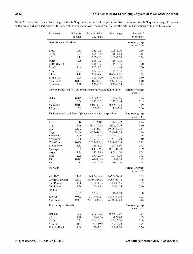
Our multisite, multi-experiment, multi-data stream DA ap-proach (Base assimilation) increased confidence in the modelparameters (Table 5). Averaged across parameters, the poste-rior 99 % quantile range from the Base assimilation was 60 %less than the prior range. The largest reduction in parameteruncertainty was for the parameters associated with light-useefficiency (alpha) and the conversion of GPP to net primaryproductivity (NPP) (y), which on average had ranges thatwere 85 % lower in the posterior than the prior. Parametersassociated with allocation and allometry had a 63 % reduc-

tion in the range while parameters associated with mortalityprocesses had a 70 % reduction in the range. Parameters asso-ciated with environmental modifiers had the least reductionin the range with a 40 % decrease. In addition to the parame-ters associated with the 3-PG model, the model process errorparameters for each data stream were well constrained withlarge reductions in the range (> 99 % decrease; SupplementalTable S2)

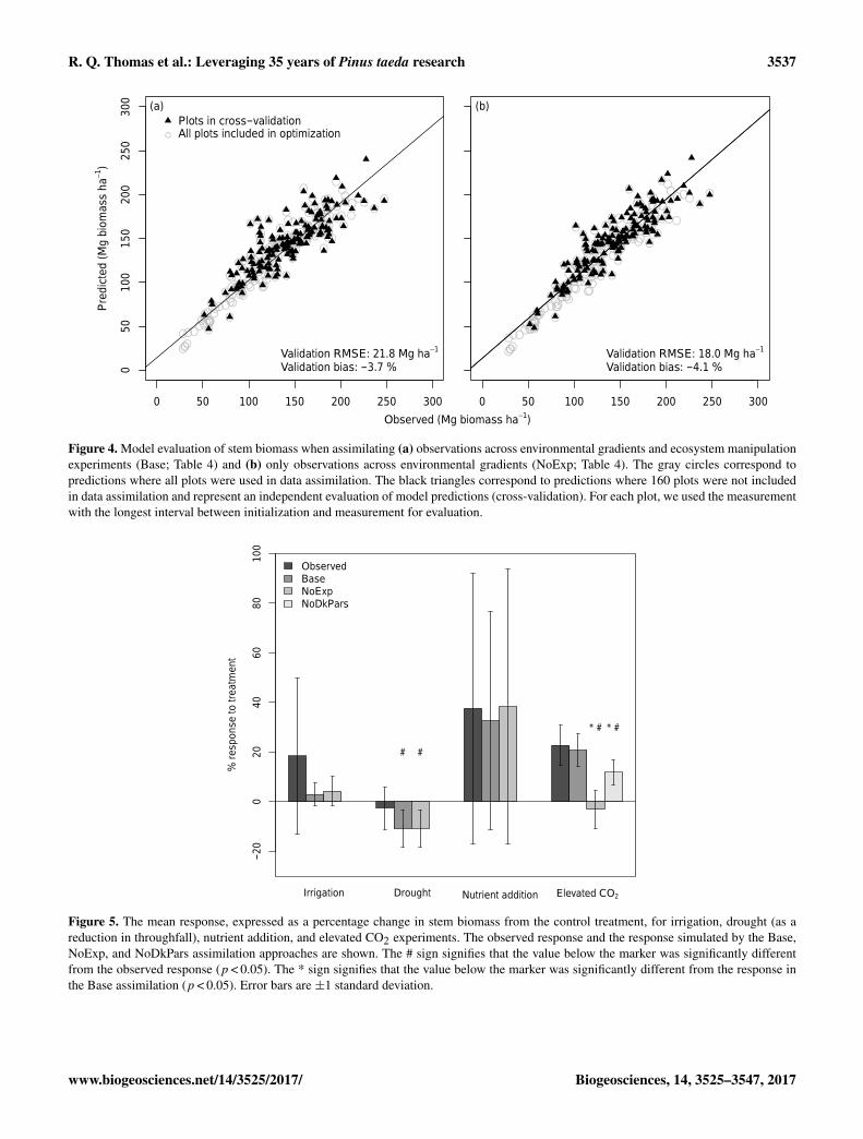
The Base assimilation reliably predicted data from theregionally distributed non-manipulated plots that were notused in the optimization. The mean bias in stem biomassof the cross-validation was −3.7 % and the RMSE was21.8 Mg ha−1 (Fig. 4a). Furthermore, the response of stembiomass to irrigation (df = 7, p = 0.18), nutrient addition(df = 26, p = 0.29), and elevated CO2 (df = 4, p = 0.43)was not significantly different between the observed and theBase assimilation (Fig. 5). The Base assimilation was sig-nificantly more sensitive to drought than observed (n= 31,p < 0.001; Fig. 5).



Table 3. The prior distributions of all 3-PG model parameters optimized using data assimilation. NPP: net primary production.

Parameter Parameter Units Prior Prior Referencedescription distribution parameters for prior

(see footnote)

Allocation and structure

pFS2 Ratio of foliage to stemallocation at stemdiameter: 2 cm

– Uniform Min: 0.08Max: 1.00

Uninformed

pFS20 Ratio of foliage to stem alloca-tion at stem diameter:20 cm


Uninformed

pRF Ratio of fine roots to foliageallocation


Uninformed

pCRS Ratio of coarse roots to stemallocation


1

SLA0 Specific leaf area at stand age 0 m2 kg−1 mean: 5.53SD: 0.44

2

SLA1 Specific leaf area for matureaged stands

m2 kg−1 Normal mean: 3.58SD: 0.11

2

tSLA Age at which specific leafarea is 0.5 (SLA0+SLA1)

Years Normal mean: 5.97SD: 2.15

2

fCpFS700 Proportional decrease in alloca-tion to foliage between 350 and700 ppm CO2


Uninformed

StemConst Constant in stem mass vs.diameter relationship

– Normal mean: 0.022SD: 0.005

3

StemPower Power in stem mass vs.diameter relationship


3

Canopy photosynthesis, autotrophic respiration, and transpiration

alpha Canopy quantum efficiency(pines)

mol C mol PAR−1 Uniform Min: 0.02Max: 0.06

Uninformed

y Ratio NPP /GPP – Uniform Min: 0.30Max: 0.65

4

MaxCond Maximum canopy conductance m s−1 Uniform Min: 0.005Max: 0.03

2

LAIgcx Canopy LAI for maximumcanopy conductance

– Uniform Min: 2Max: 5

2, 5, 6

Environmental modifiers of photosynthesis and transpiration

kF Reduction rate of productionper ◦C below zero


2

Tmin Minimum monthly mean tem-perature for photosynthesis

◦C Normal mean: 4.0SD: 2.0

2, 5, 6

Topt Optimum monthly mean tem-perature for photosynthesis


2, 5, 6

Tmax Maximum monthly mean tem-perature for photosynthesis


2, 5, 6

The plots at the Duke Forest study had a higher carryingcapacity of stem biomass before self-thinning (WSx1000),lower self-thinning rate (ThinPower), and smaller allocationto coarse root (pCRS) than values optimized from the otherplots across the region (Table 6). The DA approach with-out these three study-specific parameters (NoDkPars) pre-dicted significantly lower accumulation of stem biomass inresponse to elevated CO2 than observed (df = 4, p = 0.002;

Fig. 5). The NoDKPars assimilation optimized the CO2 fer-tilization parameter (fCalpha700) to a value that predicted45 % less light-use efficiency at 700 ppm (1.13 in NoDKParvs. 1.33 in Base; Table 6) than the Base assimilation.



Table 3. Continued.

Parameter Parameter Units Prior Prior Referencedescription distribution parameters for prior

(see footnote)

SWconst Moisture ratio deficit whendownregulation is 0.5


Uninformed

SWpower Power of moisture ratio deficit – Uniform Min: 1Max: 13

Uninformed

CoeffCond Defines stomatal response toVPD

mbar−1 Normal mean: 0.041SD: 0.003

2

fCalpha700 Proportional increase in canopyquantum efficiency between350 and 700 ppm CO2


Uninformed

MaxAge Maximum stand age used tocompute relative age

Years Uniform Min: 16Max: 200

Uninformed

nAge Power of relative age in the agemodifier


Uninformed

rAge Relative age to where age mod-ifier was 0.5


Uninformed

FR1 Fertility rating parameter 1(mean annual temperaturecoefficient)


Uninformed

FR2 Fertility rating parameter 2 (siteindex age 25 coefficient)


Uninformed

Mortality

wSx1000 Maximum stem mass per tree at1000 trees ha−1

kg tree−1 Normal mean: 235SD: 25

2, 5, 6

ThinPower Power in self-thinning law – Uniform Min: 1.0Max: 2.5

2, 5, 6

mS Fraction of mean stem biomassper tree on dying trees


Uninformed

Rttover Average monthly root turnoverrate

month−1 Uniform Min: 0.017Max: 0.042

7

MortRate Density-independent mortalityrate (pines)

month−1 Uniform Min: 0.0002Max: 0.004

Uninformed

Understory hardwoods

alpha_h Canopy quantum efficiency(understory hardwoods)

mol C mol PAR−1 Uniform Min: 0.005Max: 0.07

Uninformed

pFS_h Ratio of foliage to stem parti-oning (understory hardwoods)


Uninformed

pR_h Ratio of foliage to fine roots(understory hardwoods)

– Uniform Min: 0.05Max: 2

Uninformed

SLA_h Specific leaf area (understoryhardwoods)

m2 kg−1 Normal mean: 16SD: 3.8

8

fCalpha700_h Proportional increase in canopyquantum efficiency between350 and 700 ppm CO2 (under-story hardwood)


Uninformed

1: Albaugh et al., 2005. 2: Gonzalez-Benecke et al., 2016. 3: Gonzalez-Benecke et al., 2014. 4: DeLucia et al., 2007. 5: Bryars et al., 2013. 6: Subedi et al., 2015.7: Matamala et al., 2003. 8: LeBauer et al., 2010. Uninformed priors had large, ecologically reasonable bounds.


Excluding the experimental treatments from the data assim-ilation did not strongly influence the predictive capacity of

the model. The RMSE validation plots in NoExp assimila-tion decreased slightly compared to Base assimilation (21.8to 18.0 Mg ha−1), while the bias slightly increased (−3.7 to−4.1 %) (Fig. 4b). Excluding the experimental treatmentsresulted in a significantly lower response of stem biomass



●●●●

●●●●

●●●●

●●●●●

●

●

●●

●

●●

●

●

●●

●●

● ●

●

●

●

●●● ●

●

●

●

●

●●

●

●

●

●

●

●●

●

●

●

●●

●

●

●

●

●

●●●

●

●

●●

●

●●

●

●

●

●●●

●

●

●●

●

●●

●

●

●●

●● ●

●

●

●

●●●

●

●

●

●●

●●

●●

●

●

●●

●

●

●

●

●

●

●

●

●

●

●

●

●

●

● ●

●

●●

●

●

●● ● ●

●

●●

●

●●

●

●●

●

●●

●●

●

●●

●

●

●

●

●●

●

●

●

●●●

●●

●●

●●

●

●●●●●

●

●●

●

●●●

●●

●

●

●

●

● ●

●●

●●

●

●●

●●

●

●●

●

●

Observed (Mg biomass ha−1)

Pre

dict

ed (

Mg

biom

ass

ha−1

)

0 50 100 150 200 250 300

050

100

150

200

250

300

Pre

dict

ed (

Mg

biom

ass

ha−1

)

Observed (Mg biomass ha−1)

●

Plots in cross−validationAll plots included in optimization

●

Validation RMSE: 21.8 Mg ha−1

Validation bias: −3.7 %

(a)

●●●●

●●●●

●●●●

●●●●●

●

●

●●

●

●●

●

●

●●

●●

●●

●

●

●

●●● ●

●

●●

●

●●

●

●

●

●

●

●●

●

●

●

●●

●

●

●

●

●

●●●

●

●

● ●●

●●

●

●

●

●●●

●

●

●●

●

●●

●

●

●●

●● ●

●●

●

●●

●

●

●

●●●

●

●

●●

●

●

●

●

●

●

●

●

●

●

●

●

●

●

●

●

●

●

● ●

●

●●

●

●

●● ● ●

●

●

●●

●●

●

●

●

●

●●

●●

●

●●

●

●

●

●

●●

●

●

●

●●●

●●

●●

●

●

●

●●●●●

●

●●

●

●●

●●

●

●

●

●

●

● ●

●●

●●

●

●●

●

●

●

●●

●

●

Observed (Mg biomass ha−1)P

redi

cted

(M

g bi

omas

s ha

−1)

0 50 100 150 200 250 300

●

Validation RMSE: 18.0 Mg ha−1

Validation bias: −4.1 %

(b)

Figure 4. Model evaluation of stem biomass when assimilating (a) observations across environmental gradients and ecosystem manipulationexperiments (Base; Table 4) and (b) only observations across environmental gradients (NoExp; Table 4). The gray circles correspond topredictions where all plots were used in data assimilation. The black triangles correspond to predictions where 160 plots were not includedin data assimilation and represent an independent evaluation of model predictions (cross-validation). For each plot, we used the measurementwith the longest interval between initialization and measurement for evaluation.

Irrigation Drought Nutrient addition Elevated CO2

% r

espo

nse

to tr

eatm

ent

−20

020

4060

8010

0

ObservedBaseNoExpNoDkPars

* # * #

# #

Figure 5. The mean response, expressed as a percentage change in stem biomass from the control treatment, for irrigation, drought (as areduction in throughfall), nutrient addition, and elevated CO2 experiments. The observed response and the response simulated by the Base,NoExp, and NoDkPars assimilation approaches are shown. The # sign signifies that the value below the marker was significantly differentfrom the observed response (p < 0.05). The * sign signifies that the value below the marker was significantly different from the response inthe Base assimilation (p < 0.05). Error bars are ±1 standard deviation.



15 20 25 30 35

0.5

0.6

0.7

0.8

0.9

1.0

Site index (m)

Soi

l fer

tility

rat

ing

(FR

)

BaseNoExp

(a)

0.0 0.2 0.4 0.6 0.8 1.0

0.4

0.6

0.8

1.0

Fraction of maximium available soil water

Soi

l wat

er m

odifi

er

(b)

400 500 600 700 800 900

1.0

1.1

1.2

1.3

1.4

Atmospheric CO2 (ppm)

CO

mod

ifier

2

BaseNoexpNoDkPars

(c)

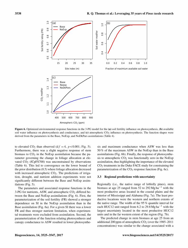
Figure 6. Optimized environmental response functions in the 3-PG model for the (a) soil fertility influence on photosynthesis, (b) availablesoil water influence on photosynthesis and conductance, and (c) atmospheric CO2 influence on photosynthesis. The function shapes werederived from the parameters in the Base, NoExp, and NoDkPars assimilations (Table 4).

to elevated CO2 than observed (df = 4, p < 0.001; Fig. 5).Furthermore, there was a slight negative response of stembiomass to CO2 in the NoExp assimilation because the pa-rameter governing the change in foliage allocation at ele-vated CO2 (fCpFS700) was unconstrained by observations(Table 6). This led to convergence on the lower bound ofthe prior distribution (0.5) where foliage allocation decreasedwith increased atmospheric CO2. The predictions of irriga-tion, drought, and nutrient addition experiments were notsignificantly different between the Base and NoExp assim-ilations (Fig. 5).

The parameters and associated response functions in the3-PG for nutrients, ASW, and atmospheric CO2 differed be-tween the Base and NoExp assimilations (Fig. 6). First, theparameterization of the soil fertility (FR) showed a strongerdependence on SI in the NoExp assimilation than in theBase assimilation (Fig. 6a). For a given SI there was a lowerFR and thus stronger nutrient limitation, when experimen-tal treatments were excluded from assimilation. Second, theparameterization of the function relating photosynthesis andcanopy conductance to ASW resulted in lower photosynthe-

sis and maximum conductance when ASW was less than50 % of the maximum ASW in the NoExp than in the Baseassimilations (Fig. 6b). Finally, the response of photosynthe-sis to atmospheric CO2 was functionally zero in the NoExpassimilation, thus highlighting the importance of the elevatedCO2 treatments in the Duke FACE study for constraining theparameterization of the CO2 response function (Fig. 6c).


Regionally (i.e., the native range of loblolly pines), stembiomass at age 25 ranged from 52 to 292 Mg ha−1 with themost productive areas located in the coastal plains and theinterior of Mississippi and Alabama (Fig. 7a). The least pro-ductive locations were the western and northern extents ofthe native range. The width of the 95 % quantile interval foreach HUC12 unit ranged from 6.2 to 29.8 Mg ha−1 with thelargest uncertainty located in the most productive HUC12units and in the far western extent of the region (Fig. 7b).

The predicted change in stem biomass at age 25 from anadditional 200 ppm of atmospheric CO2 (over the 1985–2011concentrations) was similar to the change associated with a



Figure 7. (a) Regional predictions of stem biomass stocks for a 25-year-old stand planted in 1985. Parameters used in the predictions werefrom the Base assimilation approach described in Table 5. (b) The width of the 95 % quantile interval associated with uncertainty in modelparameters.

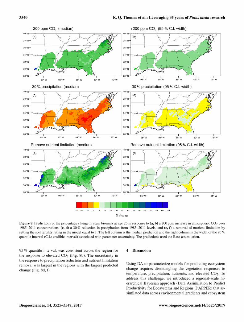
removal of nutrient limitation (by setting FR to 1) (Fig. 8a, c).The median change associated with elevated CO2 for a givenHUC12 unit ranged from 19.2 to 55.7 % with a regional me-dian of 21.7 % (Fig. 8a). The change associated with theremoval of nutrient limitation ranged from 6.9 to 303.7 %for a given HUC12 unit, with a regional median of 24.1 %(Fig. 8b). The response to elevated CO2 was more consis-tent across space than the response to nutrient addition. Thelargest potential gains in productivity from nutrient additionwere predicted in central Georgia, the northern extent of theregion, and the western extents, areas with the lowest SI(Fig. 3).

Stem biomass was considerably less responsive to a 30 %decrease in precipitation than to nutrient addition and anincrease in atmospheric CO2. The median change in stembiomass when precipitation was reduced from the 1985–2011 levels ranged from−11.6 to−0.1 % for a given HUC12unit with a regional median of −5.1% (Fig. 8c). CentralGeorgia was the most responsive to precipitation reduction,reflecting the relatively low annual precipitation and warmtemperatures (Fig. 3).

For a given location, the predicted response to elevatedCO2 had larger uncertainty than the predicted responseto precipitation reduction and nutrient limitation removal(Fig. 8c, d, f). The uncertainty, defined as the width of the



Figure 8. Predictions of the percentage change in stem biomass at age 25 in response to (a, b) a 200 ppm increase in atmospheric CO2 over1985–2011 concentrations, (c, d) a 30 % reduction in precipitation from 1985–2011 levels, and (e, f) a removal of nutrient limitation bysetting the soil fertility rating in the model equal to 1. The left column is the median prediction and the right column is the width of the 95 %quantile interval (C.I.: credible interval) associated with parameter uncertainty. The predictions used the Base assimilation.

95 % quantile interval, was consistent across the region forthe response to elevated CO2 (Fig. 8b). The uncertainty inthe response to precipitation reduction and nutrient limitationremoval was largest in the regions with the largest predictedchange (Fig. 8d, f).

4 Discussion

Using DA to parameterize models for predicting ecosystemchange requires disentangling the vegetation responses totemperature, precipitation, nutrients, and elevated CO2. Toaddress this challenge, we introduced a regional-scale hi-erarchical Bayesian approach (Data Assimilation to PredictProductivity for Ecosystems and Regions, DAPPER) that as-similated data across environmental gradients and ecosystem



Table 4. Description of the different data assimilation approachesused.

Simulation Treatments included in assimilation Numbername of

plots

Base All plots and experiments in the re-gion were used simultaneously. In-cludes unique pCRS, wSx1000, andThinPower parameters for plots inthe Duke FACE study.

294

NoExp Same as Base assimilation but ex-cluding all plots with experimen-tal manipulations. Includes controlplots that are part of experimentalstudies.

208

NoDkPars Same as Base assimilation but with-out pCRS, wSx1000, and Thin-Power parameter for plots in theDuke FACE and US-DK3 studies.

294

manipulation experiments into a modified version of the 3-PG model. Furthermore, we synthesized observations of car-bon stocks, carbon fluxes, water fluxes, vegetation structure,and vegetation dynamics that spanned 35 years of forest re-search in a region (Table 1, Fig. 1) with large and dynamiccarbon fluxes (Lu et al., 2015). By combining the DAPPERsystem with the regional set of observations, we were ableto estimate parameters in a model with high predictive ca-pacity (Fig. 4) and with quantified uncertainty on parameters(Table 5) and regional simulations (Figs. 7 and 8).

Our hierarchical approach (Eq. 7) was designed to parti-tion uncertainty among parameters, model process, and mea-surements (Hobbs and Hooten, 2015). Separating the param-eter and process uncertainty is required to estimate predic-tion intervals, as prediction intervals only include parameterand process errors (Dietze et al., 2013; Hobbs and Hooten,2015). Previous forest ecosystem DA efforts have either fo-cused on parameter uncertainty, by using measurement un-certainty as the variance term in a Gaussian cost function(Bloom and Williams, 2015; Keenan et al., 2012; Richard-son et al., 2010) or on total uncertainty by directly estimat-ing the Gaussian variance term (Ricciuto et al., 2008). Ourapproach allowed the estimation of the probability distribu-tion of forest biomass before uncertainty is added throughmeasurement. Considering that the method of DA can poten-tially have a large influence on posterior parameter distribu-tions (Trudinger et al., 2007), future research should focus oncomparing the hierarchical approach presented here to otherapproaches by using the same data constraints with alterna-tive cost functions.


The most important experimental manipulation for constrain-ing model parameters was the Duke FACE CO2 fertilizationstudy because the CO2 fertilization parameters (fCalpha700and fCpFS700) converged on the lower bounds of their priordistributions when the experiments were excluded from theassimilation. In contrast, excluding the nutrient fertilization,drought, and irrigation studies did not substantially alter thepredictive capacity of the model. This finding suggests thatdata assimilation using plots across environmental gradientsalone can constrain parameters associated with water and nu-trient sensitivity. However, regardless of whether the experi-ments were included in the assimilation, the optimized modelpredicted higher sensitivity to drought than observed, high-lighting that future studies should focus on improving thesensitivity to drought.

The 3-PG model included a highly simplified represen-tation of interactions between the water and carbon cyclesthat resulted in parameterizations that may contain assump-tions that require additional investigation. First, transpirationwas modeled as a function of a potential canopy transpira-tion that occurred if leaf area was not limiting transpiration.The LAI at which leaf area was no longer limiting was a pa-rameter that was optimized (LAIgcx in Table 5), resulting ina value of 2.2. Interestingly, this optimized value is consis-tent with the scant literature on this topic. In their analysisof multiyear measurements of transpiration in loblolly pine,Phillips and Oren (2001) observed that transpiration per unitleaf area was relatively insensitive to increases in leaf areaabove an LAI of approximately 2.5. Iritz and Lindroth (1996)reviewed transpiration data from a range of crop species andfound only small increases in transpiration above LAI of 3–4.These authors suggest that the threshold-type responses ob-served were related to the range of LAI at which self-shadingincreases most rapidly, therefore limiting increases in tran-spiration. The resulting model behavior of “flat” transpira-tion above 2.2 LAI, with gradually decreasing photosynthe-sis above that value, results in increasing water use efficiencyat higher LAI values. Second, the relationship between rela-tive ASW and the modifier of photosynthesis and transpira-tion predicted a modifier value greater than zero when therelative ASW was zero. This resulted in positive values fromphotosynthesis and transpiration when the average ASW dur-ing the month was zero. In practice, the monthly ASW wasrarely zero during simulations, which presents a challengeconstraining the shape of the ASW modifier. The priors forthe two ASW modifiers (SWconst and SWpower) had rangesthat permitted the modifier to be zero. Therefore, additionaldata are likely needed during very dry conditions to developa more physically based parameterization. Alternatively, theparameterization of a non-zero soil moisture modifier at zeroASW may be due to trees having access to water at soildepths deeper than the top 1.5 m of soil represented by the



Table 5. The optimized medians, range of the 99 % quantile intervals of the posterior distributions and the 99 % quantile range for priorswith normally distributed priors or the range of the upper and lower bounds for priors with uniform distributions. C.I.: credible interval.

Parameter Posterior Posterior 99 % Prior range Posterior/median C.I. range prior range

Allocation and structure Parameter groupmean: 0.38

pFS2 0.58 0.55–0.61 0.08–1.00 0.06pFS20 0.57 0.55–0.59 0.10–1.00 0.05pR 0.11 0.07–0.15 0.05–2.00 0.04pCRS 0.26 0.25–0.27 0.15–0.35 0.11pCRS (Duke) 0.21 0.18–0.23 0.15–0.35 0.20SLA0 8.44 7.67–9.25 4.4–6.66 0.70SLA1 2.84 2.72–2.96 3.59–4.16 0.43tSLA 4.13 3.88–4.41 0.43–11.51 0.05fCpFS700 0.74 0.60–0.90 0.50–1.00 0.60StemConst 0.022 0.009–0.035 0.009–0.035 1.00StemPower 2.78 2.29–3.27 2.25–3.29 0.95

Canopy photosynthesis, autotrophic respiration, and transpiration Parameter groupmean: 0.14

alpha 0.029 0.026–0.031 0.02–0.06 0.14y 0.50 0.47–0.53 0.30–0.65 0.15MaxCond 0.011 0.01–0.012 0.005–0.03 0.09LAIgcx 2.2 2.0–2.48 2.0–5 .0 0.16

Environmental modifiers of photosynthesis and transpiration Parameter groupmean: 0.61

kF 0.16 0.12–0.2 0.14–0.22 1.04Tmin −5.56 −8.88 to −2.69 −1.15 to 9.15 0.60Topt 23.42 21.1–26.31 19.85–30.15 0.51Tmax 39.56 34.71–44.39 32.85–43.15 0.94SWconst 1.09 0.91–1.56 0.01–1.8 0.36SWpower 8.86 3.39–12.98 1.00–13.00 0.80CoeffCond 0.036 0.029–0.043 0.034–0.048 0.91fCalpha700 1.33 1.18–1.52 1.0–1.80 0.43MaxAge 151.5 54.4–199.6 16.0–200 .0 0.79nAge 3.35 1.77–3.99 1.00–4.00 0.74rAge 2.25 0.81–2.99 0.01–3.00 0.73FR1 0.073 0.061–0.086 0.00–1.00 0.03FR2 0.17 0.15–0.19 0.0–1.0 0.04

Mortality Parameter groupmean: 0.37

wSx1000 176.9 169.6–184.4 165.6–294.4 0.15wSx1000 (Duke) 243.3 196.89–305.02 165.6–294.4 0.76ThinPower 1.68 1.60–1.78 1.00–2.5 0.12ThinPower 1.26 1.00–1.85 1.00–2.5 0.56(Duke)mS 0.52 0.37–0.71 0.10–1.00 0.38Rttover 0.023 0.017–0.031 0.017–0.042 0.55MortRate 0.001 9e-04–0.0011 2e-04–0.004 0.06

Understory hardwoods Parameter groupmean: 0.28

alpha_h 0.02 0.02–0.02 0.005–0.07 0.01pFS_h 1.78 1.54–2.06 0.2–3.0 0.19pR_h 0.21 0.06–0.43 0.05–2.00 0.19SLA_h 16.3 14.1–19.0 6.2–25.8 0.25fCalpha700_h 1.84 1.58–2.17 1.0–2.50 0.74



Table 6. Median and range of the 99 % quantile intervals of the posterior distributions for the parameters in the NoExp and NoDkParsassimilations

Parameter NoExp NoExp 99 % NoDkPars NoDkPar 99 %median range median

Allocation and structure

pFS2 0.63 0.61–0.68 0.57 0.55–0.60pFS20 0.63 0.60–0.65 0.57 0.55–0.59pR 0.11 0.06–0.16 0.11 0.08–0.15pCRS 0.29 0.27–0.30 0.26 0.25–0.27pCRS (Duke) 0.25 0.23–0.28 n/a n/aSLA0 7.47 6.57–8.41 8.56 7.73–9.32SLA1 3.00 2.88–3.12 2.89 2.79–2.99tSLA 4.75 4.30–5.26 4.12 3.90–4.38fCpFS700 0.50 0.50–0.53 0.94 0.83–1.00StemConst 0.022 0.01–0.04 0.02 0.01–0.04StemPower 2.79 2.27–3.26 2.77 2.28–3.30

Canopy photosynthesis, autotrophic respiration, and transpiration

alpha 0.030 0.028–0.033 0.029 0.026–0.031y 0.48 0.45–0.51 0.49 0.46–0.52MaxCond 0.017 0.015–0.021 0.011 0.011–0.012LAIgcx 4.4 3.9–5.0 2.1 2.0–2.5

Environmental modifiers of photosynthesis and transpiration

kF 0.15 0.11–0.20 0.16 0.11–0.20Tmin −7.8 −10.97 to −4.95 −6.04 −9.06 to −3.03Topt 21.55 19.15–24.39 22.71 20.54–25.42Tmax 40.56 36.51–45.62 39.82 35.62–44.56SWconst 0.93 0.8–1.1 1.14 0.91–1.62SWpower 6.27 2.98–11.49 7.99 3.29–12.95CoeffCond 0.041 0.034–0.047 0.036 0.030–0.042fCalpha700 1.01 1.0 0–1.06 1.15 1.10–1.25MaxAge 152.84 54.18–199.5 152.0 49.2–199.3nAge 3.36 1.93–3.99 3.36 1.89–3.99rAge 2.26 0.80–2.99 2.24 0.83–2.99FR1 0.12 0.09–0.14 0.08 0.07–0.09FR2 0.20 0.16–0.24 0.17 0.15–0.19

Mortality

wSx1000 191.6 180.2–210.2 181.32 173.26–196.32wSx1000 (Duke) 235.1 175.0–297.5 n/a n/aThinPower 1.76 1.61–1.92 1.59 1.46–1.72ThinPower (Duke) 1.42 1.01–2.02 n/a n/amS 0.54 0.33–0.80 0.50 0.25–0.71Rttover 0.019 0.02–0.03 0.022 0.017–0.030MortRate 0.0013 0.0011–0.0014 0.0011 9e-04–0.0013

Understory hardwoods

alpha_h 0.031 0.025–0.040 0.02 0.017–0.023pFS_h 2.39 1.86–2.96 1.79 1.59–2.09pR_h 0.25 0.05–0.67 0.21 0.06–0.41SLA_h 12.37 9.96–15.07 16.42 14.37–18.55fCalpha700_h 1.08 1.00–1.83 1.83 1.56–2.15

n/a: not applicable; NoDkPars assimilation did not include Duke-specific parameters.



bucket in 3-PG. Overall, it is important to view the parame-terization presented here as a phenomenological relationshipthat is consistent with observations from drought and irri-gation experiments as well as observations across regionalgradients in precipitation.

Constraining the sensitivity to atmospheric CO2 differsfrom constraining the sensitivity to ASW because, unlike themultiple constraints on water sensitivity (drought, irrigation,and gradient studies), environmental conditions created bythe few elevated CO2 plots provided unique constraint onparameters. Our finding demonstrated that DA efforts shouldtest for bias in unique ecosystem experiments before finaliz-ing a set of model parameters used in optimization. In par-ticular, we found that the parameter governing the photosyn-thetic response to elevated CO2 (fCalpha700) was substan-tially lower when all parameters were assumed to be sharedacross all plots than when the CO2 fertilization experimentwas allowed to have unique parameters. The need for thethree unique parameters at the Duke FACE study parameterscan be explained by the constraint provided by multiple datastreams and multiple plots. An assumption of the model wasthat an increase in stem biomass caused a decrease in stemdensity through self-thinning, unless the average tree stembiomass was below a parameterized threshold (WSx1000).Therefore, an increase in photosynthesis and stem biomassthrough CO2 fertilization could cause a decrease in stemdensity. For a single study, it is straightforward to simulta-neously fit the CO2 fertilization and self-thinning parame-ters to fit stem biomass and stem density observations forthe site. However, regional DA presents a challenge becausethe self-thinning parameters are well constrained by the stembiomass and stem density observations across the region butthe CO2 fertilization parameters are not. As a result of theregional DA, the self-thinning parameters caused a strongerdecrease in stem density than observed in the Duke FACEstudy. Therefore, the optimization favored a solution wherethere was a lower response to CO2 and thus a smaller de-crease in stem density. Allowing the Duke FACE study tohave unique self-thinning parameters resulted in lower ratesof self-thinning and allowed for simulated stem biomass torespond to CO2 in a way that matched the observations with-out penalizing the optimization by degrading the fit to thestem density.

Our finding that the Duke FACE study required uniqueself-thinning parameters to reduce bias in the simulated stembiomass suggests that when using DA to optimize parame-ters that are shared across plots, careful examination of pre-diction bias in key sites that provide a unique constraint oncertain parameters (like the Duke FACE) is critical. Basedon this example, we suggest that DA efforts using multiplestudies and multiple experiment types identify whether par-ticular experiments at a limited number of sites have the po-tential to uniquely constrain specific parameters. In this case,additional weight or site-specific parameters may be neededto avoid having the signal of the unique experiment over-

whelmed by the large amount of data from the other sites andexperiments. Additionally, the finding suggests that multisiteDA should consider using hierarchical approaches to predict-ing mortality, particularly because mortality is often not sim-ulated as mechanistically as growth. A hierarchical approach,where each plot has a set of mortality parameters that aredrawn from a regional distribution, could avoid having unex-plained variation in mortality rates leading to bias in the pa-rameterization of growth-related processes (i.e., growth re-sponses to CO2, drought, nutrient fertilization). The hierar-chical approach to mortality could also highlight patterns inmortality rates across a region and allow for additional inves-tigations into the mechanisms driving the patterns.


Our predictions of how stem biomass responds to elevatedCO2, nutrient addition, and drought were designed to illus-trate the capacity of the DAPPER approach to simulate theuncertainty in future predictions. By using DA, our regionalpredictions and the uncertainty are consistent with observa-tions but are associated with key caveats. First, only param-eter uncertainty was presented in the regional simulations.There is additional uncertainty associated with model pro-cess error. We showed the parameter uncertainty because itisolated the capacity to parameterize the individual environ-mental response functions in the model. Second, the responseto drought may be too strong because of the bias in the modelpredictions of the drought studies. However, there is poten-tial that the drought studies underestimated the sensitivity toASW since they are relatively short term (< 5 years) and ma-nipulate local ASW without manipulating large-scale ASW(i.e., regional water tables). Third, the large responses to nu-trient fertilization at the western and northern extents of thestudy region may be too high. The large responses are at-tributed to the low SI and the low predicted site fertility rat-ing (FRp). The low SI may be attributable to water limita-tion and temperature limitation that is not fully accounted forin the parameterization. Additional nutrient addition experi-ments in the northern and western extent along with furtherdevelopment of the representation of nutrient availability inthe 3-PG model may allow for a more robust representationof soil fertility. Finally, the baseline fertility used in our re-gional analysis was derived from an empirical model of SIthat was developed using field plots with minimal manage-ment (Sabatia and Burkhart, 2014). Subsequently our esti-mate of baseline fertility is likely on the low end of foreststands currently in production and the response to nutrientaddition may be higher than a typical stand under active man-agement.



5 Conclusions

DA is increasingly used for developing predictions fromecosystem models that include uncertainty estimation, dueto its ability to represent prior knowledge, integrate observa-tions into the parameterization, and estimate multiple com-ponents of uncertainty, including observation, parameter, andprocess representation uncertainty (Dietze et al., 2013; Luo etal., 2011; Niu et al., 2014). Our application of DA to loblollypine plantations of the southeastern US demonstrated thatthese ecosystems are well suited as a test-bed for the de-velopment of DA techniques, particularly techniques for as-similating ecosystem experiments. We found that assimilat-ing observations across environmental gradients can providesubstantial constraint on many model parameters but thatecosystem manipulative experiments, particularly elevatedCO2 studies, were critical for constraining parameters associ-ated with forest productivity in a more CO2-enriched atmo-sphere. This highlights the importance of whole-ecosystemmanipulation CO2 experiments for helping to parameterizeand evaluate ecosystem models. Finally, we present an ap-proach for the development of future predictions of forestproductivity for natural resource managers that leverage arich dataset of integrated ecosystem observations across a re-gion.

Data availability. Observations used in the DA can be found inthe following: the Duke FACE study can be found in McCarthy etal. (2010), the PINEMAP studies are available through the TerraCdatabase (http://terrac.ifas.ufl.edu), the US-DK3 eddy-flux towerdata are available through the AmeriFlux database (http://ameriflux.lbl.gov), the Waycross data can be found in Bryars et al. (2013),the US-NC2 data are available upon request from Asko Noormets,and the FMRC and FPC are available through membership withthe cooperatives. The parameter chains and 3-PG model code areavailable upon request from R. Quinn Thomas ([email protected]).SSURGO soils database can be found at https://sdmdataaccess.sc.egov.usda.gov.

The Supplement related to this article is available onlineat https://doi.org/10.5194/bg-14-3525-2017-supplement.

Competing interests. The authors declare that they have no conflictof interest.

Acknowledgements. Funding support came from USDA-NIFAProject 2015-67003-23485 and the Pine Integrated Network:Education, Mitigation, and Adaptation project (PINEMAP), aCoordinated Agricultural Project funded by the USDA NationalInstitute of Food and Agriculture, Award no. 2011-68002-30185.Additional funding support came from USDA-NIFA McIntire-Stennis Program. The Virginia Space Grant Consortium Graduate

STEM Research Fellowship Program provided partial support forAnnika L. Jersild. Computational support was provided by VirginiaTech Advanced Research Computing. This research was alsosupported by grants from the French Research Agency (MACACCANR-13-AGRO-0005 and MARIS ANR-14-CE03-0007). Wethank Luke Smallman and Mat Williams for helpful discussionsabout data assimilation, the corporate and government agencymembers of the FPC and FMRC research cooperatives for sup-porting the extensive long-term experimental and observationalplots in those datasets, and two anonymous reviewers for helpfulfeedback on the paper. This material is based upon work supportedby the US Department of Energy, Office of Science, Office ofBiological and Environmental Research, under contract numberDE-AC05-00OR22725.

Edited by: Sönke ZaehleReviewed by: two anonymous referees

References

Abatzoglou, J. T.: Development of gridded surface meteorologicaldata for ecological applications and modelling, Int. J. Climatol.,33, 121–131, https://doi.org/10.1002/joc.3413, 2013.

Albaugh, T., Fox, T., Allen, H., and Rubilar, R.: Juve-nile southern pine response to fertilization is influencedby soil drainage and texture, Forests, 6, 2799–2819,https://doi.org/10.3390/f6082799, 2015.

Albaugh, T. J., Lee Allen, H., Dougherty, P. M., and Johnsen, K. H.:Long term growth responses of loblolly pine to optimal nutrientand water resource availability, Forest Ecol. Manag., 192, 3–19,https://doi.org/10.1016/j.foreco.2004.01.002, 2004.

Albaugh, T. J., Allen, H. L., and Kress, L. W.: Rootand stem partitioning of Pinus taeda, Trees, 20, 176–185,https://doi.org/10.1007/s00468-005-0024-4, 2005.

Albaugh, T. J., Albaugh, J. M., Fox, T. R., Allen, H.L., Rubilar, R. A., Trichet, P., Loustau, D., and Lin-der, S.: Tamm Review: Light use efficiency and carbonstorage in nutrient and water experiments on major for-est plantation species, Forest Ecol. Manag., 376, 333–342,https://doi.org/10.1016/j.foreco.2016.05.031, 2016.

Allen, C. B., Will, R. E., and Jacobson, M. A.: Production efficiencyand radiation use efficiency of four tree species receiving irriga-tion and fertilization, Forest Sci., 51, 556–569, 2005.

Bartkowiak, S. M., Samuelson, L. J., McGuire, M. A., and Teskey,R. O.: Fertilization increases sensitivity of canopy stomatal con-ductance and transpiration to throughfall reduction in an 8-year-old loblolly pine plantation, Forest Ecol. Manag., 354, 87–96,https://doi.org/10.1016/j.foreco.2015.06.033, 2015.

Bloom, A. A. and Williams, M.: Constraining ecosystem carbon dy-namics in a data-limited world: integrating ecological “commonsense” in a model-data fusion framework, Biogeosciences, 12,1299–1315, https://doi.org/10.5194/bg-12-1299-2015, 2015.

Bryars, C., Maier, C., Zhao, D., Kane, M., Borders, B., Will, R., andTeskey, R.: Fixed physiological parameters in the 3-PG modelproduced accurate estimates of loblolly pine growth on sites indifferent geographic regions, Forest Ecol. Manag., 289, 501–514,https://doi.org/10.1016/j.foreco.2012.09.031, 2013.


http://terrac.ifas.ufl.edu

http://ameriflux.lbl.gov

http://ameriflux.lbl.gov

https://sdmdataaccess.sc.egov.usda.gov


https://doi.org/10.5194/bg-14-3525-2017-supplement

https://doi.org/10.1002/joc.3413

https://doi.org/10.3390/f6082799

https://doi.org/10.1016/j.foreco.2004.01.002

https://doi.org/10.1007/s00468-005-0024-4



https://doi.org/10.5194/bg-12-1299-2015



Burkhart, H. E., Cloeren, D. C., and Amateis, R. L.: Yield rela-tionships in unthinned loblolly pine plantations on cutover, site-prepared lands, South. J. Appl. For., 9, 84–91, 1985.

Carlson, C. A., Fox, T. R., Allen, H. L., Albaugh, T. J., Rubilar,R. A., and Stape, J. L.: Growth responses of loblolly pine in theSoutheast United States to midrotation applications of nitrogen,phosphorus, potassium, and micronutrients, Forest Sci., 60, 157–169, https://doi.org/10.5849/forsci.12-158, 2014.

DeLucia, E. H., Drake, J. E., Thomas, R. B., and Gonzalez-Meler,M.: Forest carbon use efficiency: is respiration a constant frac-tion of gross primary production?, Glob. Change Biol., 13, 1157–1167, https://doi.org/10.1111/j.1365-2486.2007.01365.x, 2007.

Dieguez-Aranda, U., Burkhart, H. E., and Amateis, R. L.: Dynamicsite model for loblolly pine (Pinus taeda L.) plantations in theUnited States, Forest Sci., 52, 262–272, 2006.

Dietze, M. C., LeBauer, D. S., and Kooper, R.: On improving thecommunication between models and data, Plant Cell Environ.,36, 1575–1585, https://doi.org/10.1111/pce.12043, 2013.

Ewers, B. E., Oren, R., Phillips, N., Stromgren, M., and Linder, S.:Mean canopy stomatal conductance responses to water and nu-trient availabilities in Picea abies and Pinus taeda, Tree Physiol.,21, 841–850, 2001.

Fox, A., Williams, M., Richardson, A. D., Cameron, D., Gove,J. H., Quaife, T., Ricciuto, D., Reichstein, M., Tomelleri,E., Trudinger, C. M., and Van Wijk, M. T.: The REFLEXproject: Comparing different algorithms and implementationsfor the inversion of a terrestrial ecosystem model againsteddy covariance data, Agr. Forest Meteorol., 149, 1597–1615,https://doi.org/10.1016/j.agrformet.2009.05.002, 2009.

Fox, T. R., Jokela, E. J., and Allen, H. L.: The development of pineplantation silviculture in the Southern United States, J. Forest„105, 337–347, 2007.

Gonzalez-Benecke, C. A. and Martin, T. A.: Water avail-ability and genetic effects on water relations of loblollypine (Pinus taeda) stands, Tree Physiol., 30, 376–392,https://doi.org/10.1093/treephys/tpp118, 2010.

Gonzalez-Benecke, C. A., Gezan, S. A., Albaugh, T. J., Allen,H. L., Burkhart, H. E., Fox, T. R., Jokela, E. J., Maier, C.A., Martin, T. A., Rubilar, R. A., and Samuelson, L. J.: Lo-cal and general above-stump biomass functions for loblollypine and slash pine trees, Forest Ecol. Manag., 334, 254–276,https://doi.org/10.1016/j.foreco.2014.09.002, 2014.

Gonzalez-Benecke, C. A., Teskey, R. O., Martin, T. A., Jokela,E. J., Fox, T. R., Kane, M. B., and Noormets, A.: Regionalvalidation and improved parameterization of the 3-PG modelfor Pinus taeda stands, Forest Ecol. Manag., 361, 237–256,https://doi.org/10.1016/j.foreco.2015.11.025, 2016.

Hobbs, N. T. and Hooten, M. B.: Bayesian Models: A StatisticalPrimer for Ecologists, Princeton University Press, Princeton, NJ,USA, 2015.

Iritz, Z. and Lindroth, A.: Energy partitioning in relation toleaf area development of short-rotation willow coppice, Agr.Forest Meteorol., 81, 119–130, https://doi.org/10.1016/0168-1923(95)02306-2, 1996.

Keenan, T. F., Carbone, M. S., Reichstein, M., and Richard-son, A. D.: The model–data fusion pitfall: assuming cer-tainty in an uncertain world, Oecologia, 167, 587–597,https://doi.org/10.1007/s00442-011-2106-x, 2011.

Keenan, T. F., Davidson, E., Moffat, A. M., Munger, W., andRichardson, A. D.: Using model-data fusion to interpret pasttrends, and quantify uncertainties in future projections, of terres-trial ecosystem carbon cycling, Glob. Change Biol., 18, 2555–2569, https://doi.org/10.1111/j.1365-2486.2012.02684.x, 2012.

Landsberg, J. and Waring, R.: A generalised model of forest produc-tivity using simplified concepts of radiation-use efficiency, car-bon balance and partitioning, Forest Ecol. Manag., 95, 209–228,https://doi.org/10.1016/S0378-1127(97)00026-1, 1997.

Le Quéré, C., Moriarty, R., Andrew, R. M., Canadell, J. G., Sitch, S.,Korsbakken, J. I., Friedlingstein, P., Peters, G. P., Andres, R. J.,Boden, T. A., Houghton, R. A., House, J. I., Keeling, R. F., Tans,P., Arneth, A., Bakker, D. C. E., Barbero, L., Bopp, L., Chang,J., Chevallier, F., Chini, L. P., Ciais, P., Fader, M., Feely, R. A.,Gkritzalis, T., Harris, I., Hauck, J., Ilyina, T., Jain, A. K., Kato,E., Kitidis, V., Klein Goldewijk, K., Koven, C., Landschützer,P., Lauvset, S. K., Lefèvre, N., Lenton, A., Lima, I. D., Metzl,N., Millero, F., Munro, D. R., Murata, A., Nabel, J. E. M. S.,Nakaoka, S., Nojiri, Y., O’Brien, K., Olsen, A., Ono, T., Pérez,F. F., Pfeil, B., Pierrot, D., Poulter, B., Rehder, G., Rödenbeck,C., Saito, S., Schuster, U., Schwinger, J., Séférian, R., Steinhoff,T., Stocker, B. D., Sutton, A. J., Takahashi, T., Tilbrook, B., vander Laan-Luijkx, I. T., van der Werf, G. R., van Heuven, S., Van-demark, D., Viovy, N., Wiltshire, A., Zaehle, S., and Zeng, N.:Global Carbon Budget 2015, Earth Syst. Sci. Data, 7, 349–396,https://doi.org/10.5194/essd-7-349-2015, 2015.

LeBauer, D. S., Dietze, M., Kooper, R., Long, S., Mulrooney, P.,Rohde, G. S., and Wang, D.: Energy Biosciences Institute, Uni-versity of Illinois at Urbana-Champaign, Biofuel Ecophysiolog-ical Traits and Yields Database (BETYdb), available at: https://www.betydb.org (last access: 16 May 2016), 2010.

Lu, X., Lu, X., Kicklighter, D. W., Kicklighter, D., Melillo, J. M.,Melillo, J. M., Reilly, J. M., Reilly, J. M., Xu, L., and Wu,L.: Land carbon sequestration within the conterminous UnitedStates: Regional- and state-level analyses, J. Geophys. Res.-Biogeo., 120, 379–398, https://doi.org/10.1002/2014JG002818,2015.

Luo, Y., Weng, E., Wu, X., Gao, C., Zhou, X., and Zhang, L.:Parameter identifiability, constraint, and equifinality in data as-similation with ecosystem models, Ecol. Appl., 19, 571–574,https://doi.org/10.1890/08-0561.1, 2009.

Luo, Y., Ogle, K., Tucker, C., Fei, S., Gao, C., LaDeau, S.,Clark, J. S., and Schimel, D. S.: Ecological forecasting anddata assimilation in a data-rich era, Ecol. Appl., 21, 1429–1442,https://doi.org/10.1890/09-1275.1, 2011.

MacBean, N., Peylin, P., Chevallier, F., Scholze, M., and Schür-mann, G.: Consistent assimilation of multiple data streams in acarbon cycle data assimilation system, Geosci. Model Dev., 9,3569–3588, https://doi.org/10.5194/gmd-9-3569-2016, 2016.

Matamala, R., Gonzàlez-Meler, M. A., Jastrow, J. D., Norby, R.J., and Schlesinger, W. H.: Impacts of fine root turnover on for-est NPP and soil C sequestration potential, Science, 302, 1385–1387, https://doi.org/10.1126/science.1089543, 2003.

McCarthy, H. R., Oren, R., Johnsen, K. H., Gallet-Budynek,A., Pritchard, S. G., Cook, C. W., LaDeau, S. L., Jackson,R. B., and Finzi, A. C.: Re-assessment of plant carbon dy-namics at the Duke free-air CO2 enrichment site: interac-tions of atmospheric [CO2] with nitrogen and water avail-


https://doi.org/10.5849/forsci.12-158

https://doi.org/10.1111/j.1365-2486.2007.01365.x

https://doi.org/10.1111/pce.12043

https://doi.org/10.1016/j.agrformet.2009.05.002

https://doi.org/10.1093/treephys/tpp118



https://doi.org/10.1016/0168-1923(95)02306-2

https://doi.org/10.1016/0168-1923(95)02306-2

https://doi.org/10.1007/s00442-011-2106-x

https://doi.org/10.1111/j.1365-2486.2012.02684.x

https://doi.org/10.1016/S0378-1127(97)00026-1

https://doi.org/10.5194/essd-7-349-2015

https://www.betydb.org

https://www.betydb.org

https://doi.org/10.1002/2014JG002818

https://doi.org/10.1890/08-0561.1

https://doi.org/10.1890/09-1275.1

https://doi.org/10.5194/gmd-9-3569-2016

https://doi.org/10.1126/science.1089543


ability over stand development, New Phytol., 185, 514–528,https://doi.org/10.1111/j.1469-8137.2009.03078.x, 2010.

McKeand, S., Mullin, T., Byram, T., and White, T.: Deploymentof genetically improved loblolly and slash pines in the south, J.Forest., 101, 32–37, 2003.

Medlyn, B. E., Zaehle, S., De Kauwe, M. G., Walker, A. P., Di-etze, M. C., Hanson, P. J., Hickler, T., Jain, A. K., Luo, Y., Par-ton, W., Prentice, I. C., Thornton, P. E., Wang, S., Wang, Y.-P., Weng, E., Iversen, C. M., McCarthy, H. R., Warren, J. M.,Oren, R., and Norby, R. J.: Using ecosystem experiments to im-prove vegetation models, Nature Climate Change, 5, 528–534,https://doi.org/10.1038/nclimate2621, 2015.

Niu, S., Luo, Y., Dietze, M. C., Keenan, T. F., Shi, Z., Li, J.,and Chapin III, F. S.: The role of data assimilation in pre-dictive ecology, Ecosphere, 5, 65, https://doi.org/10.1890/ES13-00273.1, 2014.

Noormets, A., Gavazzi, M. J., McNulty, S. G., Domec, J.-C., Sun, G., King, J. S., and Chen, J.: Response of car-bon fluxes to drought in a coastal plain loblolly pine forest,Glob. Change Biol., 16, 272–287, https://doi.org/10.1111/j.1365-2486.2009.01928.x, 2010.

Novick, K. A., Oishi, A. C., Ward, E. J., Siqueira, M. B. S., Juang,J.-Y., and Stoy, P. C.: On the difference in the net ecosystem ex-change of CO2 between deciduous and evergreen forests in thesoutheastern United States, Glob. Change Biol., 21, 827–842,https://doi.org/10.1111/gcb.12723, 2015.

Oren, R., Ellsworth, D., Johnsen, K., Phillips, N., Ewers, B., Maier,C., Schafer, K., McCarthy, H., Hendrey, G., McNulty, S. G.,and Katul, G.: Soil fertility limits carbon sequestration by forestecosystems in a CO2-enriched atmosphere, Nature, 411, 469–472, https://doi.org/10.1038/35078064, 2001.

Pan, Y., Birdsey, R. A., Fang, J., Houghton, R., Kauppi, P. E., Kurz,W. A., Phillips, O. L., Shvidenko, A., Lewis, S. L., Canadell,J. G., Ciais, P., Jackson, R. B., Pacala, S. W., McGuire, A. D.,Piao, S. L., Rautiainen, A., Sitch, S., and Hayes, D.: A large andpersistent carbon sink in the world’s forests, Science, 333, 988–993, https://doi.org/10.1126/science.1201609, 2011.

Phillips, N. and Oren, R.: Intra- and inter-annual variation in tran-spiration of a pine forest, Ecol. Appl., 11, 385–396, 2001.

Raymond, J. E., Fox, T. R., Strahm, B. D., and Zerpa, J.: Differ-ences in the recovery of four different nitrogen containing fertil-izers after two application seasons in pine plantations across thesoutheastern United States, Forest Ecol. Manag., 380, 161–171,https://doi.org/10.1016/j.foreco.2016.08.044, 2016.

Ricciuto, D. M., Davis, K. J., and Keller, K.: A Bayesian calibra-tion of a simple carbon cycle model: The role of observations inestimating and reducing uncertainty, Glob. Biogeochem. Cy., 22,GB2030, https://doi.org/10.1029/2006GB002908, 2008.

Richardson, A. D., Williams, M., Hollinger, D. Y., Moore, D. J.P., Dail, D. B., Davidson, E. A., Scott, N. A., Evans, R. S.,Hughes, H., Lee, J. T., Rodrigues, C., and Savage, K.: Estimat-ing parameters of a forest ecosystem C model with measurementsof stocks and fluxes as joint constraints, Oecologia, 164, 25–40,https://doi.org/10.1007/s00442-010-1628-y, 2010.

Sabatia, C. O. and Burkhart, H. E.: Predicting siteindex of plantation loblolly pine from biophysi-cal variables, Forest Ecol. Manag., 326, 142–156,https://doi.org/10.1016/j.foreco.2014.04.019, 2014.

Samuelson, L. J., Butnor, J., Maier, C., Stokes, T. A., Johnsen, K.,and Kane, M.: Growth and physiology of loblolly pine in re-sponse to long-term resource management: defining growth po-tential in the southern United States, Can. J. Forest Res., 38, 721–732, https://doi.org/10.1139/X07-191, 2008.

Shvidenko, A., Barber, C. V., and Persson, R.: Forest and WoodlandSystems, in: Ecosystems and Human Well-being Current Stateand Trends, Volume, edited by: Hassan, R., Scholes, R., and Ash,N., 585–621, Island Press, Washington, USA, 2005.

Soil Survey Staff: Natural Resources Conservation Service, UnitedStates Department of Agriculture, Soil Survey Geographic(SSURGO) Database, available online at: https://sdmdataaccess.sc.egov.usda.gov, last access: 12 November 2013.

Subedi, S., Fox, T., and Wynne, R.: Determination of fertility rating(FR) in the 3-PG model for loblolly pine plantations in the South-eastern United States based on site index, Forests, 6, 3002–3027,https://doi.org/10.3390/f6093002, 2015.

Tang, Z., Sayer, M. A. S., Chambers, J. L., and Barnett, J.P.: Interactive effects of fertilization and throughfall exclu-sion on the physiological responses and whole-tree carbon up-take of mature loblolly pine, Can. J. Botany, 82, 850–861,https://doi.org/10.1139/b04-064, 2004.

Trudinger, C. M., Raupach, M. R., Rayner, P. J., Kattge, J., Liu,Q., Pak, B., Reichstein, M., Renzullo, L., Richardson, A. D.,Roxburgh, S. H., Styles, J., Wang, Y.-P., Briggs, P., Barrett,D., and Nikolova, S.: OptIC project: An intercomparison ofoptimization techniques for parameter estimation in terrestrialbiogeochemical models, J. Geophys. Res., 112, G02027–17,https://doi.org/10.1029/2006JG000367, 2007.

Ward, E. J., Domec, J.-C., Laviner, M. A., Fox, T. R., Sun,G., McNulty, S., King, J., and Noormets, A.: Fertilization in-tensifies drought stress: Water use and stomatal conductanceof Pinus taeda in a midrotation fertilization and through-fall reduction experiment, Forest Ecol. Manag., 355, 72–82,https://doi.org/10.1016/j.foreco.2015.04.009, 2015.

Weng, E. and Luo, Y.: Relative information contributions of modelvs. data to short- and long-term forecasts of forest carbon dy-namics, Ecol. Appl., 21, 1490–1505, https://doi.org/10.1890/09-1394.1, 2011.

Will, R., Fox, T., Akers, M., Domec, J.-C., González-Benecke, C.,Jokela, E., Kane, M., Laviner, M., Lokuta, G., Markewitz, D.,McGuire, M., Meek, C., Noormets, A., Samuelson, L., Seiler,J., Strahm, B., Teskey, R., Vogel, J., Ward, E., West, J., Wilson,D., and Martin, T.: A range-wide experiment to investigate nu-trient and soil moisture interactions in loblolly pine plantations,Forests, 6, 2014–2028, https://doi.org/10.3390/f6062014, 2015.

Williams, M., Schwarz, P., Law, B. E., Irvine, J., and Kurpius,M.: An improved analysis of forest carbon dynamics us-ing data assimilation, Glob. Change Biol., 11, 89–105,https://doi.org/10.1111/j.1365-2486.2004.00891.x, 2005.

Zobitz, J. M., Desai, A. R., Moore, D. J. P., and Chadwick, M.A.: A primer for data assimilation with ecological models usingMarkov Chain Monte Carlo (MCMC), Oecologia, 167, 599–611,https://doi.org/10.1007/s00442-011-2107-9, 2011.

Ziehn, T., Scholze, M., and Knorr, W.: On the capability of montecarlo and adjoint inversion techniques to derive posterior param-eter uncertainties in terrestrial ecosystem models, Global Bio.-Geochem. Cy., 26, GB3025, doi:10.1029/2011GB004185, 2012.


https://doi.org/10.1111/j.1469-8137.2009.03078.x

https://doi.org/10.1038/nclimate2621

https://doi.org/10.1890/ES13-00273.1

https://doi.org/10.1890/ES13-00273.1

https://doi.org/10.1111/j.1365-2486.2009.01928.x

https://doi.org/10.1111/j.1365-2486.2009.01928.x

https://doi.org/10.1111/gcb.12723

https://doi.org/10.1038/35078064

https://doi.org/10.1126/science.1201609


https://doi.org/10.1029/2006GB002908

https://doi.org/10.1007/s00442-010-1628-y


https://doi.org/10.1139/X07-191



https://doi.org/10.3390/f6093002

https://doi.org/10.1139/b04-064

https://doi.org/10.1029/2006JG000367


https://doi.org/10.1890/09-1394.1

https://doi.org/10.1890/09-1394.1

https://doi.org/10.3390/f6062014

https://doi.org/10.1111/j.1365-2486.2004.00891.x

https://doi.org/10.1007/s00442-011-2107-9

leveraging 35 years of pinus taeda research in the...

Documents