let2015 national conference seminar
TRANSCRIPT

Webアプリケーションで学ぶ統計解析の基礎と応用
外国語教育メディア学会(LET) 第55回全国研究大会セミナー 2015/08/04@千里ライフサイエンスセンター
水本 篤(関西大学)

自己紹介

前田・山森(編著)(2004)
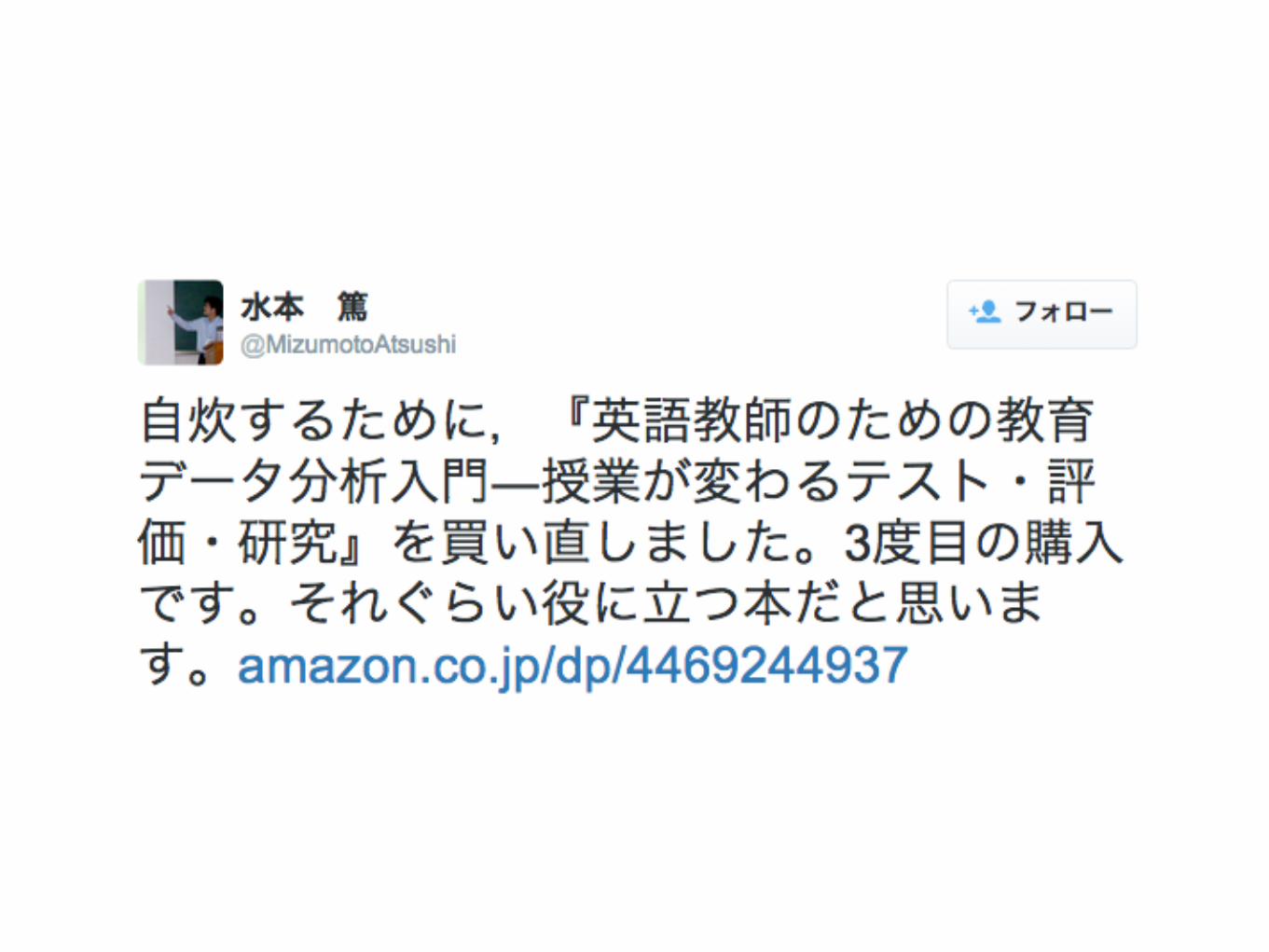

竹内・水本(編著)(2012)

•院生や初学者にもわかる本。 •前田・山森(編著)(2004)の発展版。 •新しい統計手法の紹介。 •質的研究に対するモヤモヤ感。
執筆の背景

amazon のレビュー
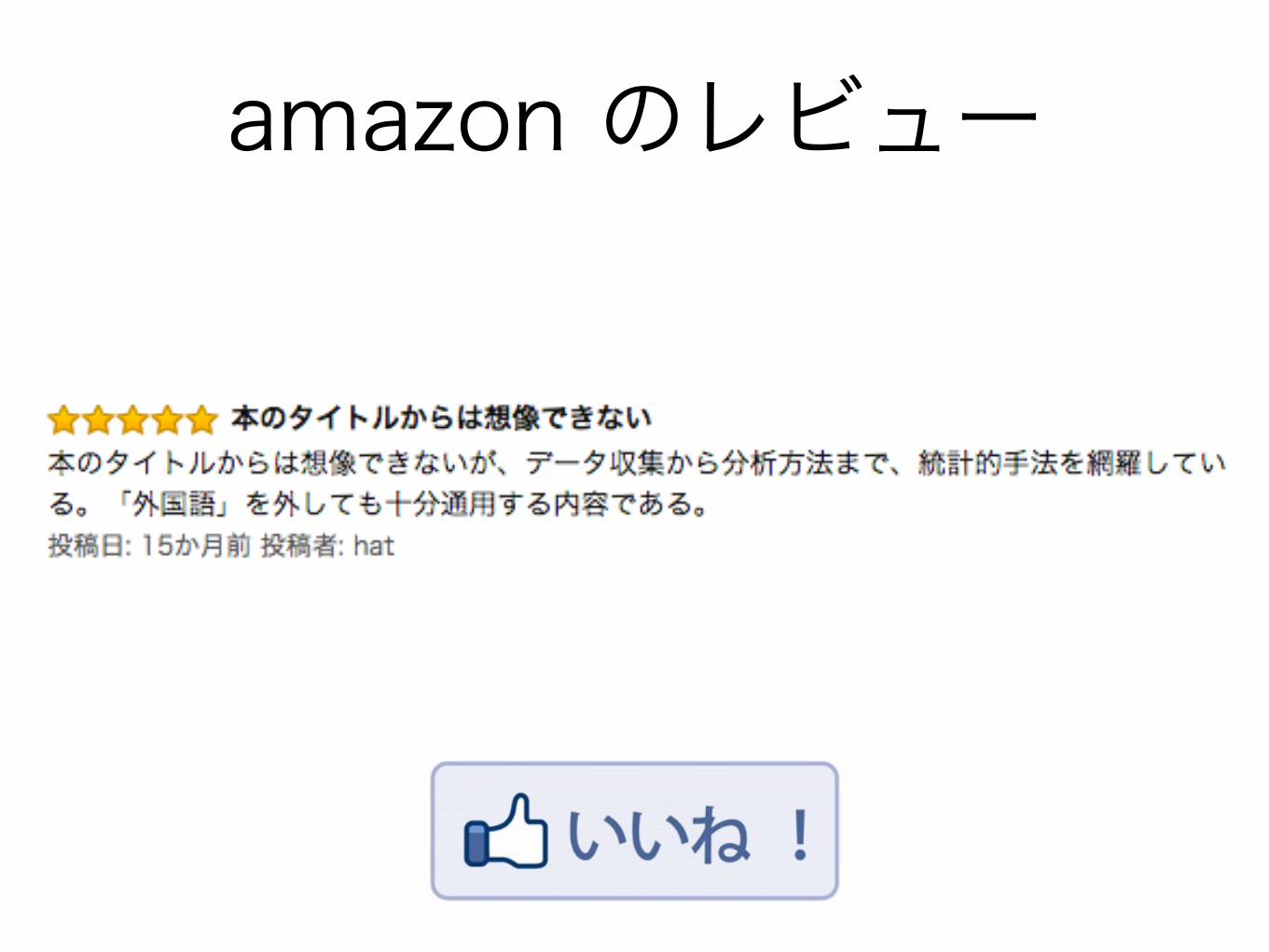
amazon のレビュー

(個人的に)嬉しいこと

"Thank you very much." Dr. Hiroaki "Keiroh" Maeda (1974–2014).
He will be remembered always and forever.

もう一つの"売り"


•MS Excel(できるものだけ) • IBM SPSS • フリーのデータ解析環境R

•MS Excel(できるものだけ) • IBM SPSS • フリーのデータ解析環境R
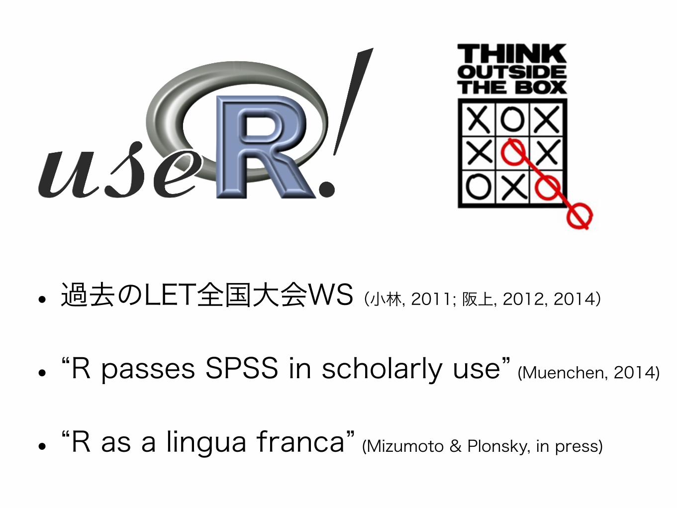
•過去のLET全国大会WS(小林, 2011; 阪上, 2012, 2014) • “R passes SPSS in scholarly use” (Muenchen, 2014) • “R as a lingua franca” (Mizumoto & Plonsky, in press)

ただ... RはCLI

RをGUIで利用できるhttp://socserv.mcmaster.ca/jfox/Misc/Rcmdr/Rcmdr-screenshot.html
R Commander(EZR)など
http://www.jichi.ac.jp/saitama-sct/SaitamaHP.files/statmedEN.html

https://sites.google.com/site/casualmacr/home
RをGUIで利用できるMac用アプリのMacR


さらに一歩進んで便利(というか楽)なのがWebアプリケーション


普段Rでやってること
•csvやxlsなどで元データを準備
•Rにデータを読み込む
•パッケージの関数を使って分析

• ハンドブックの量的チャプターのサンプルを使用して再現できる。
• アウトプットの見方がわかる • 自分でも簡単に分析できる。 • グラフを充実させている。 • Excelのデータをコピペするだけ。
langtest.jp

ここにExcelからデータをコピペするだけ

行列もいける。

パス図も


注意点•誰でもできる… だけに危険。
•ドキュメンテーションがない。
•サーバでRを走らせているので少し重い。
•自由度ゼロ(要望が有り次第改善予定)。
•コードが残らないので再現性に乏しい。

Photo Credit: JD Hancock via Compfight cc
本当の狙い

• 学部生,修士課程の院生「ハンドブック」の分析をハンズオンで実行し,卒論,修論の分析で利用。
• 博士課程の院生,量的研究を行う研究者分析方法の確認,コードを見て自分でRを使う。(langtest.jp だけでは不十分と感じるはずなので)
対象と目的https://www.dashingd3js.com/assets/steep_learning_curve-7c6e27560aabbd16a3ddb4eca06fe2fb.jpg


Demo

•国際ジャーナルで最近求められているクオリティー。
• LET機関誌でも求められているクオリティー。
これから説明する内容

1. 記述統計(平均と標準偏差)
2. 統計的検定
3. 効果量と信頼区間
4. 検定力分析
統計解析の基礎的知識

1. 記述統計(平均と標準偏差)
2. 統計的検定
3. 効果量と信頼区間
4. 検定力分析
統計解析の基礎的知識

• 平均値(mean: M)
• 標準偏差(standard deviation: SD)
記述統計 (descriptive statistics)

母集団と標本
母集団
(未知)
標 本
(既知)推定
データ解析
Σ, F, t, p...
http://www.urano-ken.com/blog/2013/08/05/let2013-workshop/
記述統計の説明の前に大事な概念

母集団μ = 15.3
標本A M = 14.7
標本BM = 15.9
標本C M = 15.2
標本DM = 15.4
標本EM = 15.1 http://www.urano-ken.com/blog/2013/08/05/let2013-workshop/
標本ごとに実現値は違う

母集団μ = ?
標本A M = 14.7
http://www.urano-ken.com/blog/2013/08/05/let2013-workshop/
実際はM = μとして推定

母集団μ = ?
実際はM = μとして推定
ScoreFrequency
30 40 50 60 70 80
05
1015
20
M = 50.59

•ある標本で得られた代表値(e.g., 平均)と母集団の代表値との差
•標本のサイズが大きければ大きいほど、標本誤差は小さくなる
•つまり推定の精度が高くなる
http://www.urano-ken.com/blog/2013/08/05/let2013-workshop/
標本誤差

平均値と標準偏差


平均値と分散(標準偏差)
0 20 40 60 80
20
30
40
50
60
Person (n = 92)
Score
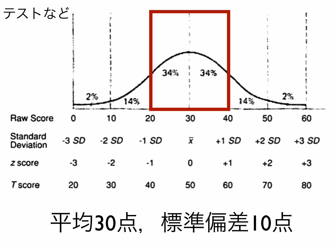
平均30点,標準偏差10点
テストなど

平均2.8点,標準偏差1.2点
2.8
質問紙など
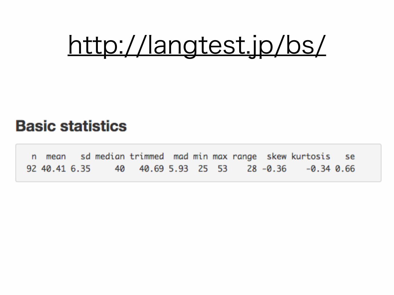

M = 40.41, SD = 6.35


• たとえば,1つのクラス
• 人数 40名
• 平均 64.1点
• 標準偏差 6.85点
どういう分布をイメージしますか?

• 平均 64.1点
• 標準偏差 6.85点
Normal Distribution
40 50 60 70 80 90

実際のデータ
• 平均 64.1点
• 標準偏差 6.85点

• 平均と標準偏差で表したデータ
• 要約としてはわかりやすいがすべての情報は保てない
• 手元のデータの要約というよりは,母集団の「きれいな」分布のイメージ
• 必ずグラフで確認する!
注意点

1. 記述統計(平均と標準偏差)
2. 統計的検定
3. 効果量と信頼区間
4. 検定力分析
統計解析の基礎的知識

1. 記述統計(平均と標準偏差)
2. 統計的検定
3. 効果量と信頼区間
4. 検定力分析
統計解析の基礎的知識

母集団と標本(推測統計)
母集団
(未知)
標 本
(既知)推定
データ解析
Σ, F, t, p...
http://www.urano-ken.com/blog/2013/08/05/let2013-workshop/

(t)検定のロジック• 2つのグループには「差がない」と仮定 • 2つのグループの人数,平均値,標準偏差から
t 値を算出
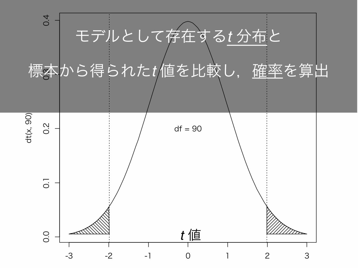
• モデルとして存在するt 分布と標本から得られたt 値を比較し,確率を算出
• 「差がない」確率が p < .05 なら有意差あり

母集団
2つのグループには「差がない」
Score
Frequency
20 40 60 80 100
05
1015
Score
Frequency
20 40 60 80 1000
510
1520
=「同じ母集団から抽出された標本である」

(t)検定のロジック• 2つのグループには「差がない」と仮定 • 2つのグループの人数,平均値,標準偏差から
t 値を算出
• モデルとして存在するt 分布と標本から得られたt 値を比較し,確率を算出
• 「差がない」確率が p < .05 なら有意差あり

t 値
※人数,平均値,分散(標準偏差の2乗) しか入っていないことに注目!
等分散の仮定が満たされる場合

(t)検定のロジック• 2つのグループには「差がない」と仮定 • 2つのグループの人数,平均値,標準偏差から
t 値を算出
• モデルとして存在するt 分布と標本から得られたt 値を比較し,確率を算出
• 「差がない」確率が p < .05 なら有意差あり
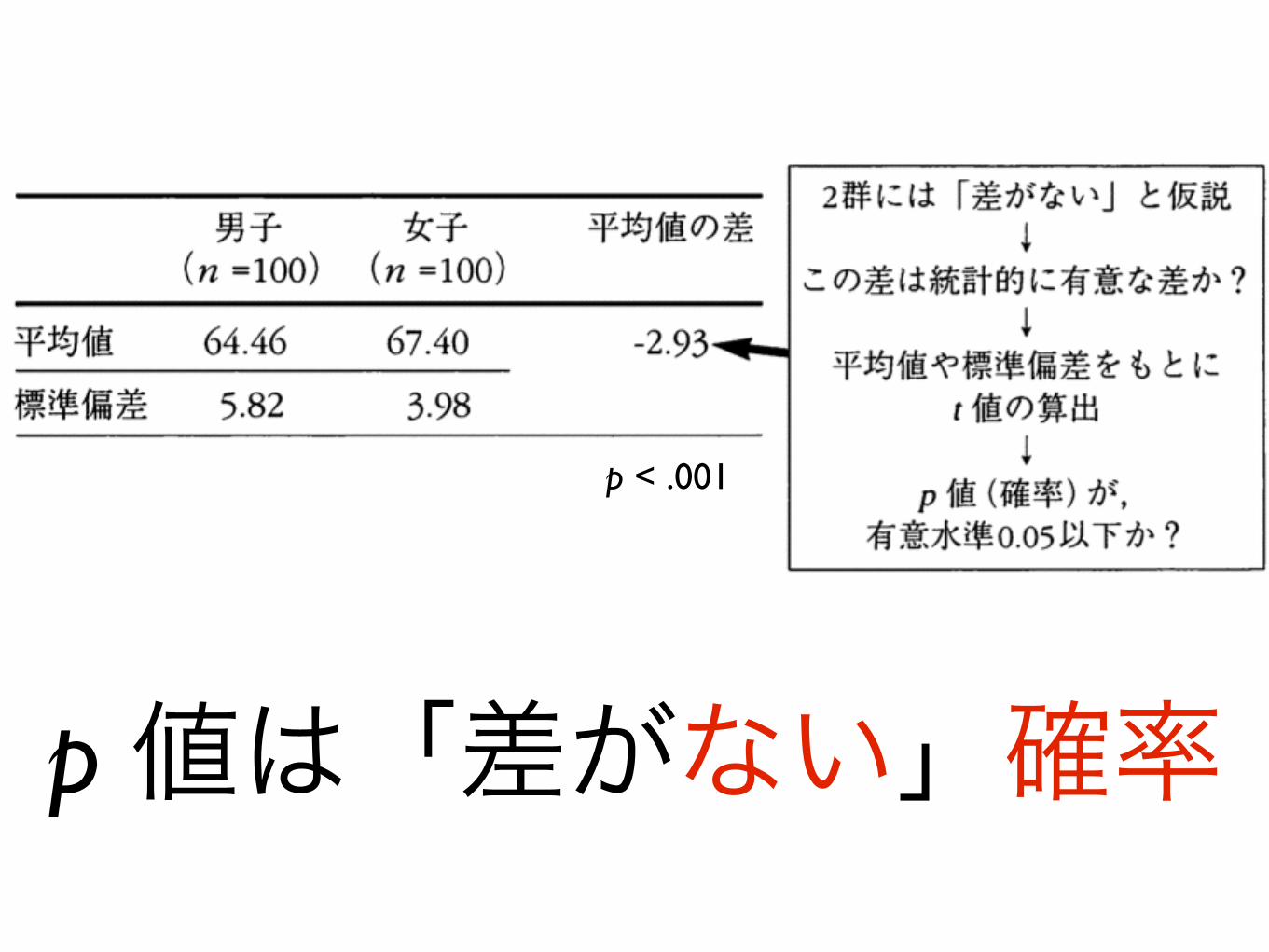
p 値は「差がない」確率
p < .001

p = .03(3%) p < .05(0.05以下)
p < .05 であれば統計的に有意な差あり
p 値は「差がない」確率
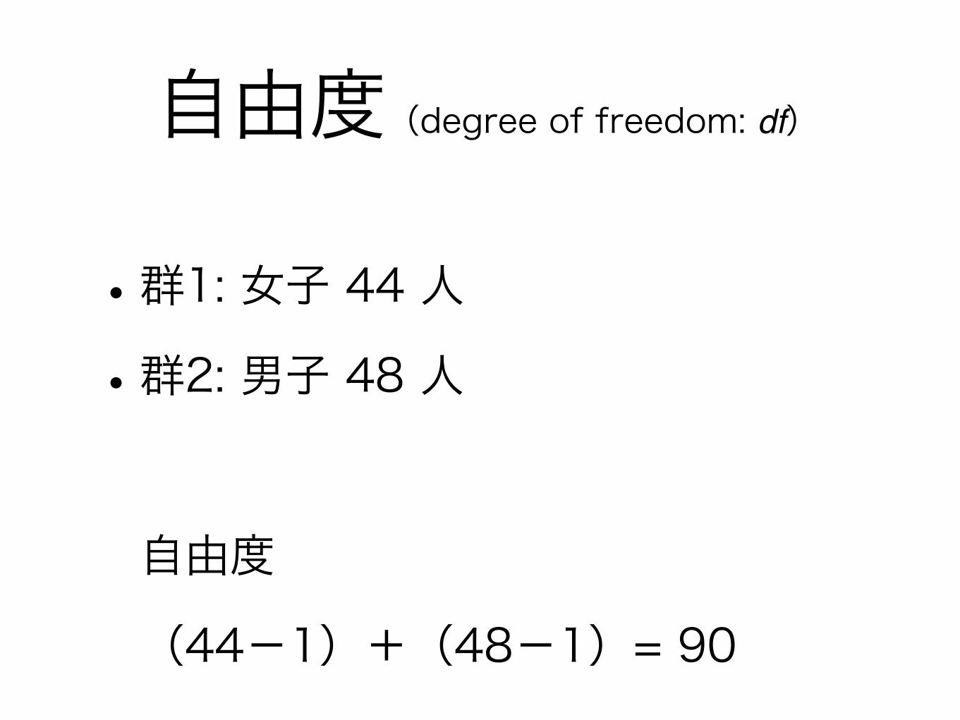
自由度(degree of freedom: df)
•群1: 女子 44 人 •群2: 男子 48 人
自由度
(44-1)+(48-1)= 90

-3 -2 -1 0 1 2 3
0.0
0.1
0.2
0.3
0.4
x
dt(x, 90)
df = 90
t 値
-3 -2 -1 0 1 2 3
0.0
0.1
0.2
0.3
0.4
x
dt(x, 90)
df = 90
モデルとして存在するt 分布と
標本から得られたt 値を比較し,確率を算出
t 値

結果の見方・報告
p < .05(0.05以下)
•p < .05 であれば統計的に有意な差あり。
•p > .05 であれば統計的に有意な差なし。
•書き方 t (90) = 0.09, p = .93

Demo“Learning by doing stats”
http://langtest.jp/tut/
“Comparing Two Independent Samples”http://langtest.jp/two/

1. 記述統計(平均と標準偏差)
2. 統計的検定
3. 効果量と信頼区間
4. 検定力分析
統計解析の基礎的知識

1. 記述統計(平均と標準偏差)
2. 統計的検定
3. 効果量と信頼区間
4. 検定力分析
統計解析の基礎的知識

統計的に有意な
p < .05(0.05以下)
statistically significant

前田・山森(編著)(2004)「有意差は差の大小については何も語ってくれません。差の大きさを見たいときは,平均値の違いそのものを見ましょう。」(p. 34)

Cumming (2012)
ストップ p 値信仰APA 6th (2009) 大久保・岡田 (2009)
「統計改革」
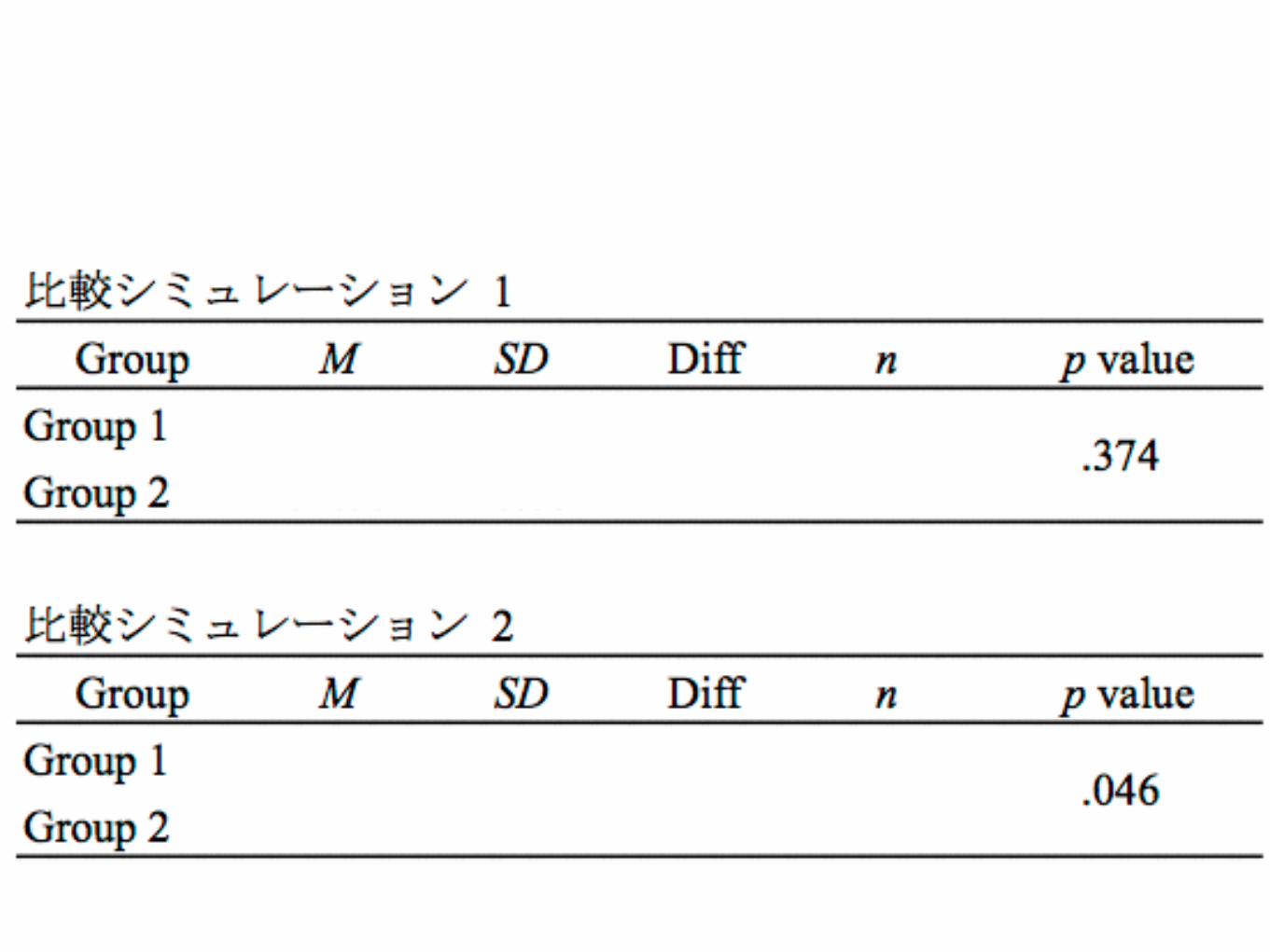


p = .046(p < .05)
N = 400
たったの2点差!

• 統計的検定の問題点- サンプルサイズが影響。- 有意差あり・なしのみの判断。- p 値は実質的な差を示さない。
効果量(Effect Size)

• 効果量(Effect Size)- サンプルサイズに影響されない。- 効果の大小を示す。- 実質的な差を確認できる。
• APA 6th では報告が「不可欠」

各群の人数が等しい場合
p 値を算出するための検定統計量との関係
検定統計量 = 効果量 (d) × サンプルサイズ
(南風原, 2002, p. 163)
詳しくは浦野(2013)を参照。http://www.slideshare.net/uranoken/let2013workshop

M = 30SD = 10

M = 30SD = 10
M = 32SD = 10

M = 30SD = 10
M = 32SD = 102/10 = 0.2
d = 0.2 (効果量小)

M = 30SD = 10
M = 35SD = 105/10 = 0.5
d = 0.5 (効果量中)

M = 30SD = 10
M = 38SD = 108/10 = 0.8
d = 0.8 (効果量大)

Plonsky and Oswald(2014)
• d = 0.40, small effect
• d = 0.70, medium effect
• d = 1.00, large effect
“L2 field-specific benchmarks”
*For pre-post and within-group contrasts:d = 0.60 (small), 1.00 (medium), 1.40 (large)
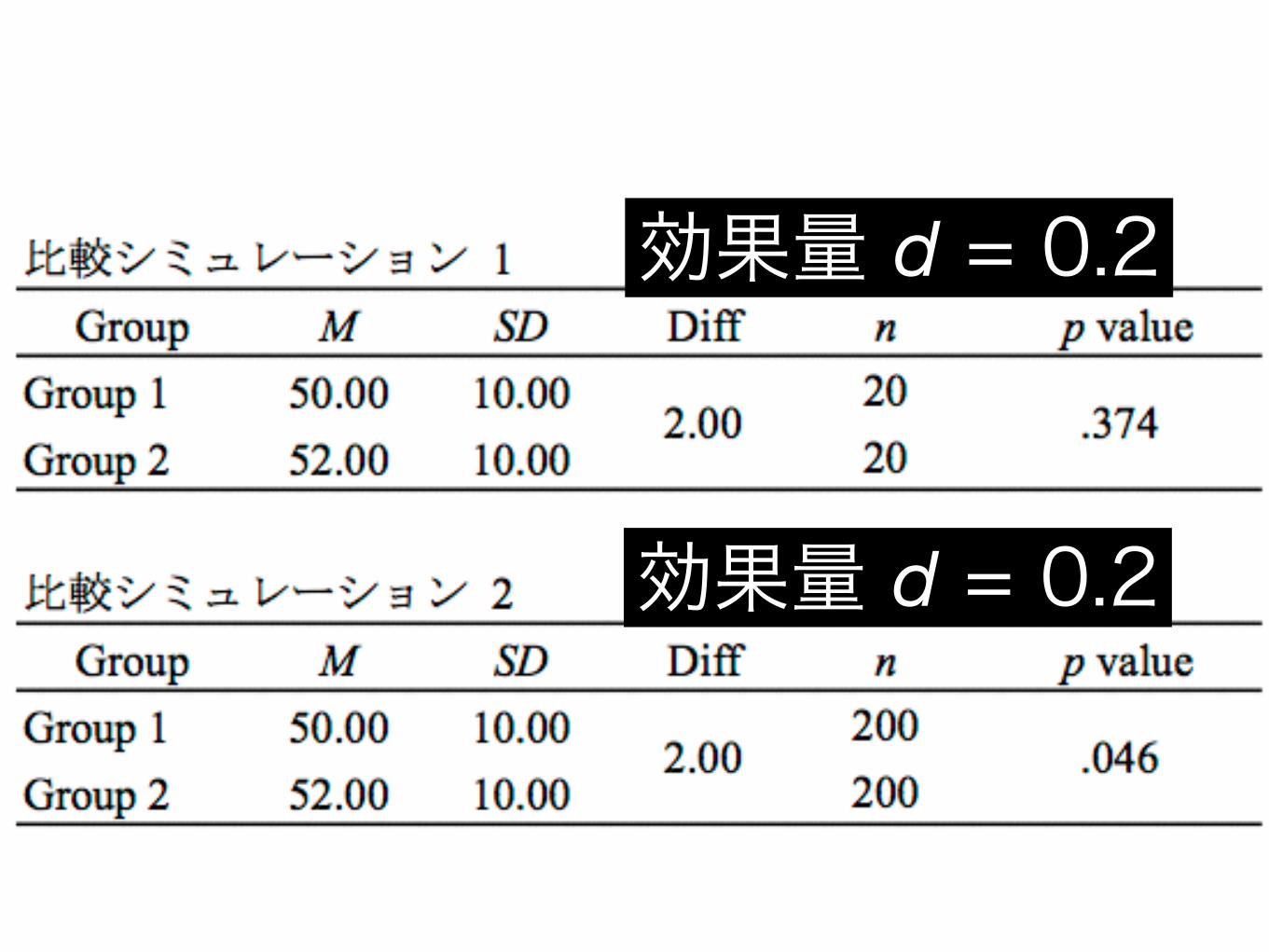
効果量 d = 0.2
効果量 d = 0.2

•(帰無仮説検定の場合)+αの情報量
• 再現性がある。
• 点推定は「過剰評価」しがち。 区間推定が研究積み上げの基本。
効果量の信頼区間も報告Confidence Interval

95%信頼区間のイメージ
-1.5 -1.0 -0.5 0.0 0.5 1.0 1.5
020
4060
80100
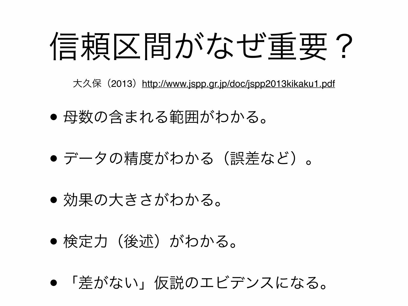
• 母数の含まれる範囲がわかる。
• データの精度がわかる(誤差など)。
• 効果の大きさがわかる。
• 検定力(後述)がわかる。
• 「差がない」仮説のエビデンスになる。
信頼区間がなぜ重要?大久保(2013)http://www.jspp.gr.jp/doc/jspp2013kikaku1.pdf

RE Model
-2.00 0.00 2.00 4.00 6.00
Standardized Mean Difference
Study63Study62Study61Study60Study59Study58Study57Study56Study55Study54Study53Study52Study51Study50Study49Study48Study47Study46Study45Study44Study43Study42Study41Study40Study39Study38Study37Study36Study35Study34Study33Study32Study31Study30Study29Study28Study27Study26Study25Study24Study23Study22Study21Study20Study19Study18Study17Study16Study15Study14Study13Study12Study11Study10Study09Study08Study07Study06Study05Study04Study03Study02Study01
1.03 [ 0.66 , 1.39 ]-0.09 [ -0.56 , 0.38 ] 0.18 [ -0.34 , 0.71 ] 0.66 [ 0.31 , 1.01 ] 0.69 [ 0.23 , 1.16 ] 1.37 [ 1.01 , 1.73 ] 1.69 [ 1.32 , 2.06 ] 0.95 [ 0.48 , 1.42 ] 0.41 [ 0.05 , 0.77 ] 0.44 [ 0.08 , 0.80 ] 0.08 [ -0.27 , 0.44 ] 2.23 [ 1.84 , 2.62 ] 1.09 [ 0.76 , 1.42 ] 1.23 [ 0.89 , 1.56 ] 1.42 [ 0.88 , 1.96 ] 1.10 [ 0.61 , 1.59 ] 1.49 [ 0.98 , 2.01 ] 0.91 [ 0.54 , 1.28 ] 1.43 [ 0.63 , 2.23 ] 0.55 [ 0.19 , 0.91 ] 0.37 [ 0.00 , 0.74 ] 1.52 [ 1.11 , 1.93 ] 1.14 [ 0.75 , 1.54 ] 0.44 [ -0.02 , 0.90 ] 0.65 [ 0.21 , 1.10 ] 0.14 [ -0.30 , 0.59 ] 0.05 [ -0.39 , 0.49 ] 0.45 [ -0.01 , 0.91 ] 0.62 [ 0.17 , 1.07 ] 0.33 [ -0.12 , 0.77 ] 0.20 [ -0.24 , 0.64 ] 1.96 [ 1.31 , 2.61 ] 0.23 [ -0.17 , 0.63 ] 0.21 [ -0.19 , 0.61 ] 0.50 [ 0.10 , 0.90 ] 1.26 [ 0.83 , 1.70 ] 0.60 [ 0.19 , 1.01 ] 0.65 [ 0.06 , 1.24 ] 0.42 [ -0.13 , 0.97 ] 0.16 [ -0.42 , 0.74 ]-0.01 [ -0.59 , 0.57 ] 0.43 [ -0.16 , 1.02 ]-0.11 [ -0.69 , 0.47 ] 0.80 [ 0.10 , 1.50 ] 1.49 [ 0.74 , 2.24 ] 0.58 [ -0.10 , 1.27 ] 1.18 [ 0.46 , 1.89 ] 0.55 [ 0.10 , 0.99 ] 0.18 [ -0.26 , 0.62 ]-0.15 [ -0.67 , 0.38 ] 0.40 [ -0.13 , 0.93 ] 2.14 [ -0.32 , 4.60 ] 2.65 [ 1.21 , 4.08 ] 3.89 [ 2.11 , 5.67 ] 0.37 [ -0.35 , 1.10 ] 0.00 [ -0.60 , 0.60 ] 0.51 [ -0.11 , 1.12 ] 0.35 [ 0.04 , 0.65 ] 0.33 [ 0.02 , 0.64 ] 0.66 [ 0.06 , 1.25 ] 0.34 [ -0.24 , 0.91 ] 4.12 [ 3.23 , 5.01 ] 1.41 [ 0.85 , 1.98 ]
0.76 [ 0.59 , 0.93 ]
Effect Size [95%CI]Study
効果量の統合=メタ分析

http://www.mizumot.com/stats/effectsize.xls
http://langtest.jp/効果量と信頼区間も計算してくれる
効果量計算シートは信頼区間の算出なし

• Yes and no. - サンプリングの影響- p 値は再現性がない(unreliable) - しかし数十年は使用される...
統計的検定は必要ない?
• 効果量とその信頼区間を 併せて報告
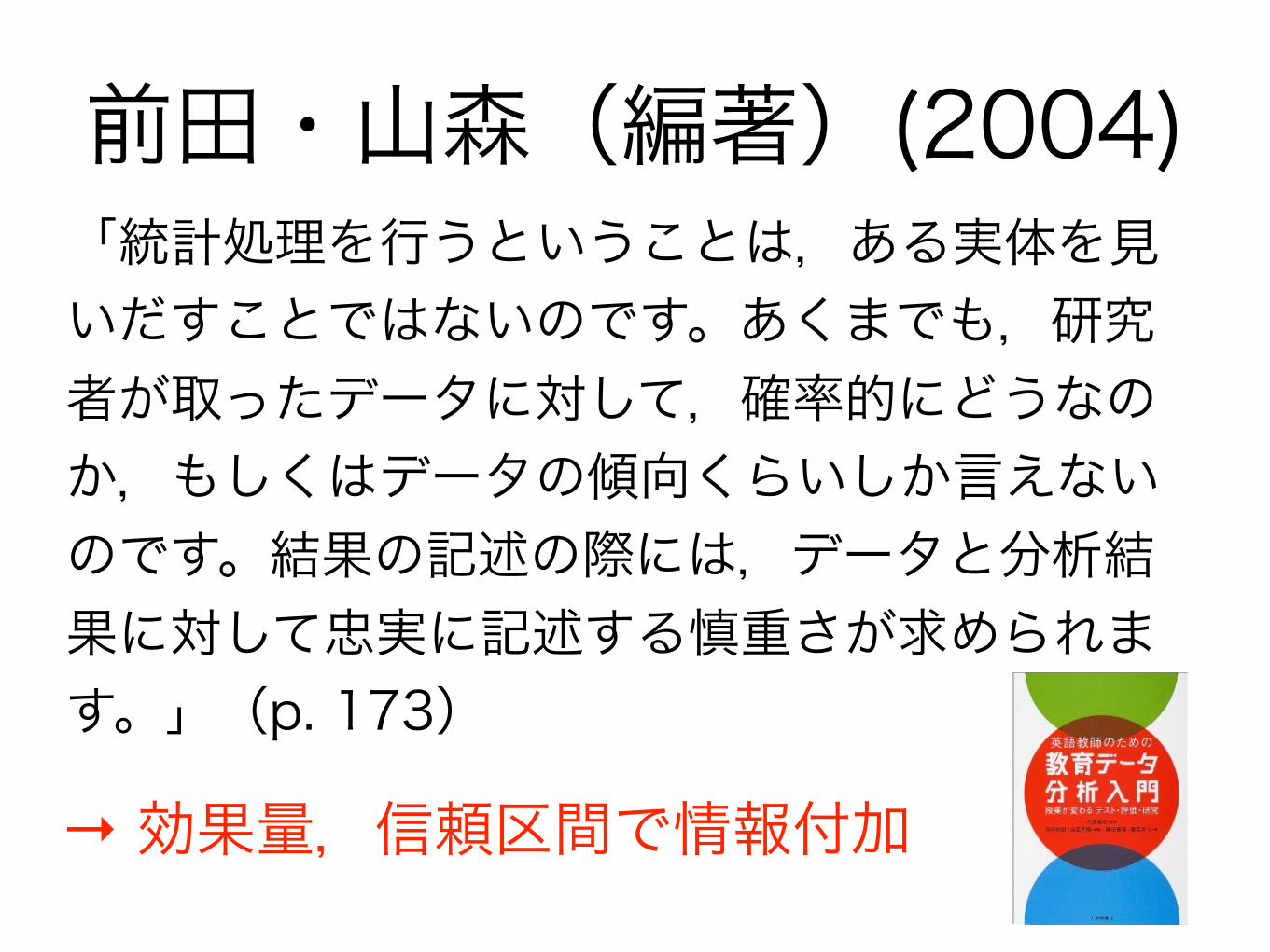
前田・山森(編著)(2004)「統計処理を行うということは,ある実体を見いだすことではないのです。あくまでも,研究者が取ったデータに対して,確率的にどうなのか,もしくはデータの傾向くらいしか言えないのです。結果の記述の際には,データと分析結果に対して忠実に記述する慎重さが求められます。」(p. 173)
→ 効果量,信頼区間で情報付加

The Basic and Applied Social Psychology
http://www.tandfonline.com/doi/abs/10.1080/01973533.2015.1012991#.Vb3tuJPtlBd
p値(帰無仮説検定)禁止!

Demo“Comparing Two Independent Samples”
http://langtest.jp/two/
“Meta-analysis”http://langtest.jp/meta/

1. 記述統計(平均と標準偏差)
2. 統計的検定
3. 効果量と信頼区間
4. 検定力分析
統計解析の基礎的知識

1. 記述統計(平均と標準偏差)
2. 統計的検定
3. 効果量と信頼区間
4. 検定力分析
統計解析の基礎的知識

同じ条件
同じ参加者数(サンプルサイズ)
同じ平均値の差(効果量)
p 値は再現性がない
→ Cumming (2012) の Excelシートでシミュレーションhttp://www.latrobe.edu.au/psy/research/cognitive-and-developmental-psychology/esci

2群の比較,各群32名,効果量 d = 0.5

2群の比較,各群32名,効果量 d = 0.5

• シミュレーション- 1つのグループに32名(計64名)- d は 0.5(効果量中)- p < .05 となったのは50%程度
d = 0.5 なのに有意差なし?
→ 検定力(power)が足りない

• 本当に差がある場合に,有意差を検出することができる力。
• 0 ~ 1の範囲の値(100%)
• Cohen (1988) は 0.8 (80%) を提唱。
検定力(statistical power)

• シミュレーション- 1つのグループに32名(計64名)- d は 0.5(効果量中)- p < .05 となったのは50%程度
先ほどの例

2群の比較,各群32名,効果量 d = 0.5

本当は差があるはずなのに= d は 0.5(効果量中)
p < .05 となったのは50%程度
検定力 = 0.5

• 本当に差がある場合に,有意差を検出することができる力。
• 検定力0.5の場合は半分の場合,「差がない」と判断されてしまう。
• もう少し噛み砕いて言うと,「p < .05の結果を得られる再現性」。
検定力(statistical power)

検定力(power)を大きくし,できるだけ小さなサンプルサイズで効率良く検定するために,必要なサンプルサイズを見積もる方法。
検定力分析(power analysis)

•有意水準 (α)
•サンプルサイズ•効果量•検定力
統計的検定における4つの要素
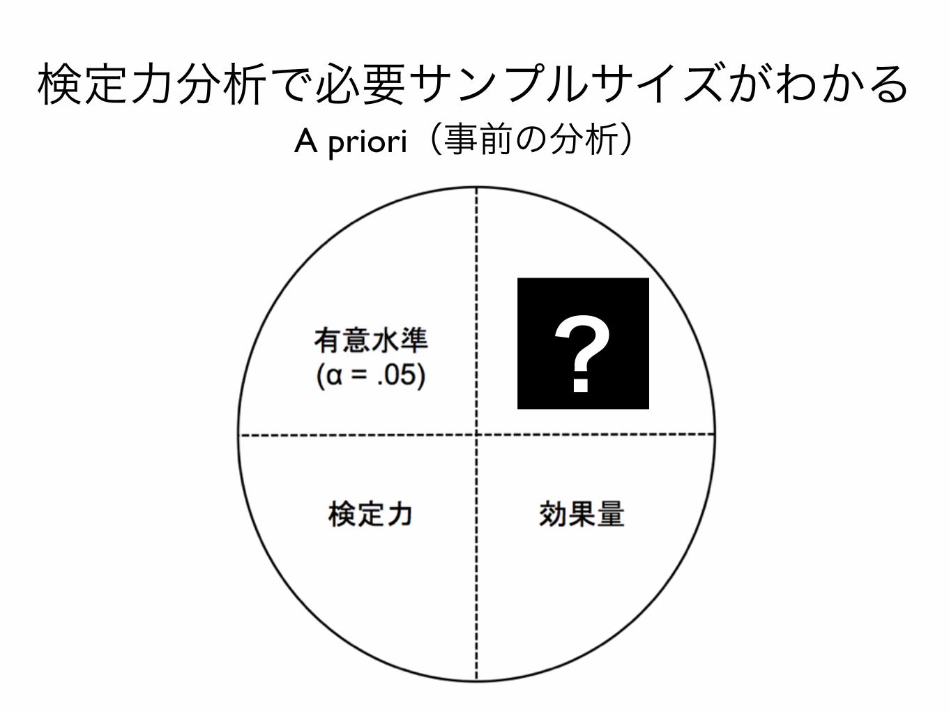
検定力分析で必要サンプルサイズがわかる
?
A priori(事前の分析)


検定力を推奨されている0.8にしたい
?
0.8 小,中,大

検定力 0.8で1群につき64名必要

2群の比較,各群32名,効果量 d = 0.5
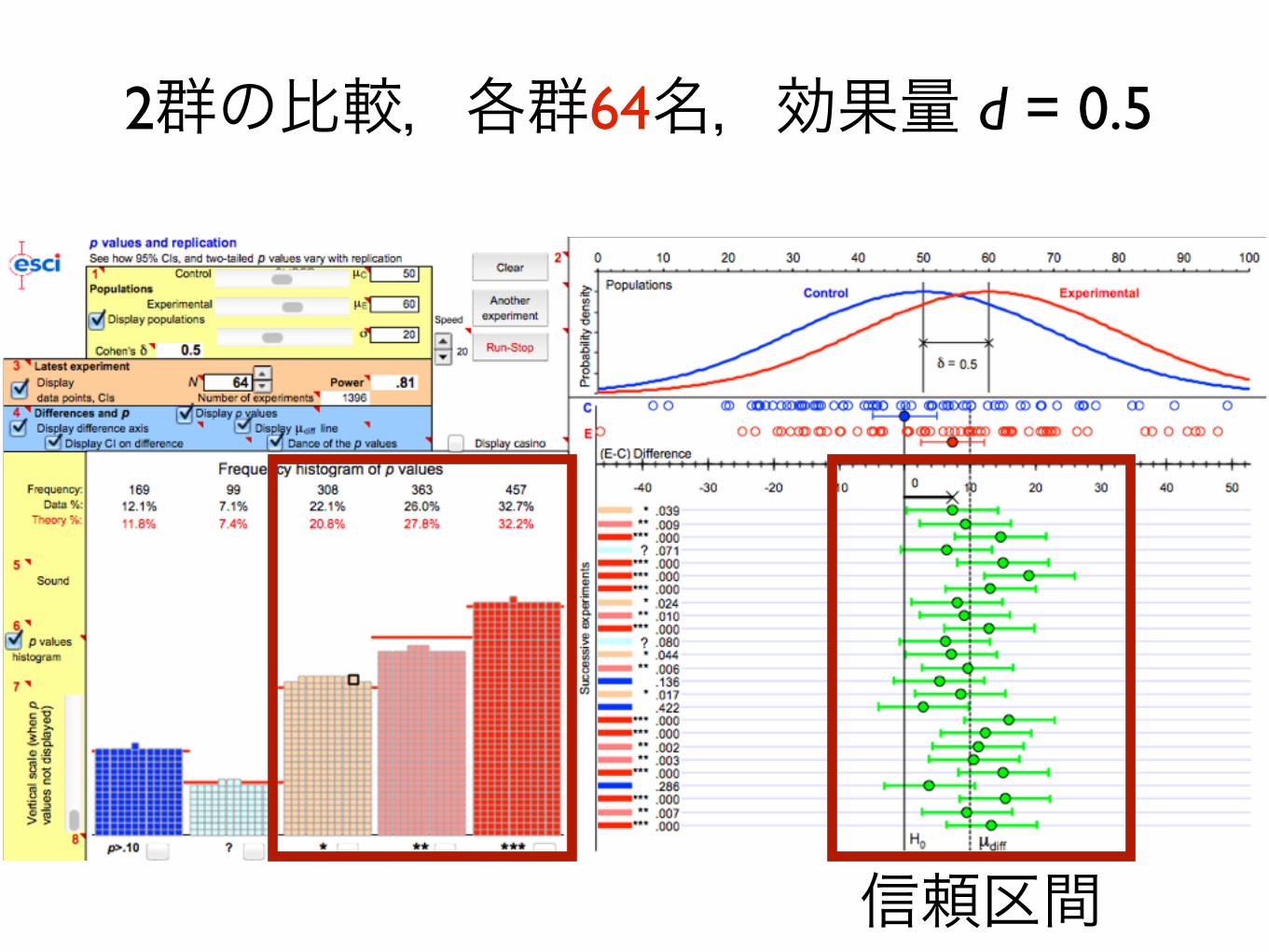
2群の比較,各群64名,効果量 d = 0.5
信頼区間

検定力分析はなぜ広まらないのか?
•研究者(特に指導者)の理解・認識不足•ワンショットの研究が多い•「独創的な研究」が求められる•対象トピックの先行研究が少ない→ Replicationをもっと推奨すべき

Porte (2012)

•検定力分析の信頼区間バージョン。
•信頼区間の幅を先に決めておいて,サンプルサイズ設計を行う。
•RのMBESSパッケージ
http://cran.r-project.org/web/packages/MBESS/http://www3.nd.edu/~kkelley/site/MBESS.html
Precision Analysis(正確度分析)AIPE: accuracy in parameter estimation

• p 値は再現性を考えるとひどい指標。
• 実質的な差や効果は「効果量」。• 信頼区間がベター(結果を蓄積)。• 先行研究からどの程度の効果があるか推測する。(もしくはメタ分析を行う)
• サンプルサイズ設計には検定力分析。
1回の研究で断言できることはほぼない!

Photo Credit: write_adam via Compfight cc
もっとReplication(追試)やメタ分析マインドを!

Replication や メタ分析に
必要な情報を書く

前田・山森(編著)(2004)
「必要な情報はきちんと書く。情報は追試できるように書く。読者にわかりやすく書く。」(p. 172)

déjà-vu
「結果は図3に示した。プリテストとポストテストの間で8.2点の得点上昇があり,統計的にも有意な上昇であった(t(11) = 9.108, p <. 01, 両側検定)。」

「ダメ。ゼッタイ。」
•平均・標準偏差の記載なし。•人数・総数が不明。•信頼性係数などの報告なし。•p 値のみの報告。(* がたくさん。)

(分析の)追試に必要な情報
•サンプルサイズ,平均, 標準偏差
•相関係数(対応ありデータ,SEMなど)
•信頼性係数(平均への回帰,相関の希薄化の修正など)

1. L2研究における「統計改革」
2. 結果と分析の再現性・透明性の重視
その他に知っておくべきこと

1. L2研究における「統計改革」
2. 結果と分析の再現性・透明性の重視
その他に知っておくべきこと

L2研究における「統計改革」
•「統計改革」がL2研究でも進んでいる。
• 各ジャーナルで Editorial や Guideline,特別号に方針が掲載されている。
http://onlinelibrary.wiley.com/doi/10.1111/lang.2015.65.issue-S1/issuetoc

L2研究における「統計改革」Larson-Hall, J., & Plonsky, L. (2015). Reporting and interpreting quantitative research findings: What gets reported and recommendations for the field. Language Learning, 65/Supp. 1, 125–157. doi:10.1111/lang.12115
1. 記述統計報告の改善
2. 効果量とその信頼区間の報告
3. 測定道具の信頼性の報告
4. データ可視化の重視
5. データの公開

L2研究における「統計改革」Larson-Hall, J., & Plonsky, L. (2015). Reporting and interpreting quantitative research findings: What gets reported and recommendations for the field. Language Learning, 65/Supp. 1, 125–157. doi:10.1111/lang.12115
1. 記述統計報告の改善
2. 効果量とその信頼区間の報告
3. 測定道具の信頼性の報告
4. データ可視化の重視
5. データの公開

まずい図の例
40#
45#
50#
55#
60#
65#
70#
75#
10 20 40
CALL

まずい図の例22%#
18%#
13%#
13%#
9%#
11%#
14%#
「なんかExcelの3Dグラフかっこいいからやってみました」http://www.clas.kitasato-u.ac.jp/~fujiwara/infoScienceA/chooseGraph/chooseGraph.html
http://jikitourai.net/dont-use-piechart

サンプルをまねる
Figure 2.4 (p. 19) in Nicol, A. A. M., & Pexman, P. M. (2010) Displaying your findings: A practical guide for creating figures, posters, and presentations (6th ed.). Washington, DC: American Psychological Association.

「隠れる」「隠される」 情報がない
0
10
20
30
40
50
60
70
80
90
100
10 20 40
CALL
***
***
BetterNot so good

138
個別のデータも見せる
Much better
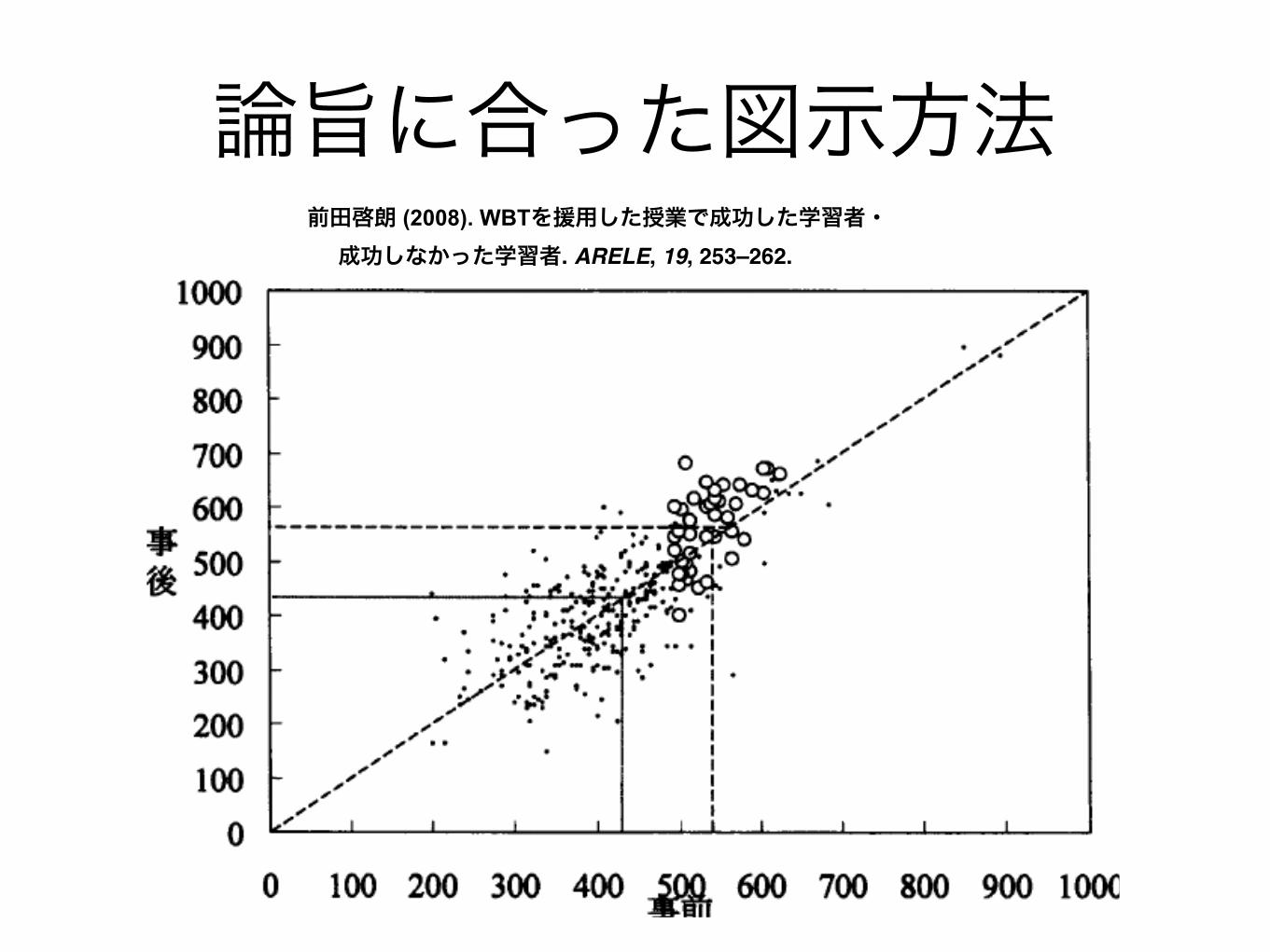
論旨に合った図示方法前田啓朗 (2008). WBTを援用した授業で成功した学習者・ 成功しなかった学習者. ARELE, 19, 253–262.

おすすめhttp://www.slideshare.net/Kunihiro_KUSANAGI/2013-ws

L2研究における「統計改革」Larson-Hall, J., & Plonsky, L. (2015). Reporting and interpreting quantitative research findings: What gets reported and recommendations for the field. Language Learning, 65/Supp. 1, 125–157. doi:10.1111/lang.12115
1. 記述統計報告の改善
2. 効果量とその信頼区間の報告
3. 測定道具の信頼性の報告
4. データ可視化の重視
5. データの公開

1. L2研究における「統計改革」
2. 結果と分析の再現性・透明性の重視
その他に知っておくべきこと

再現性は研究の基本
• データの二次利用を推奨すべき。例えば,使用したデータを(個人情報に気をつけて)オンラインなどで公開。
• Rなどのコードも 公開すれば,誰でも再現可能。


http://onlinelibrary.wiley.com/doi/10.1111/lang.12134/full
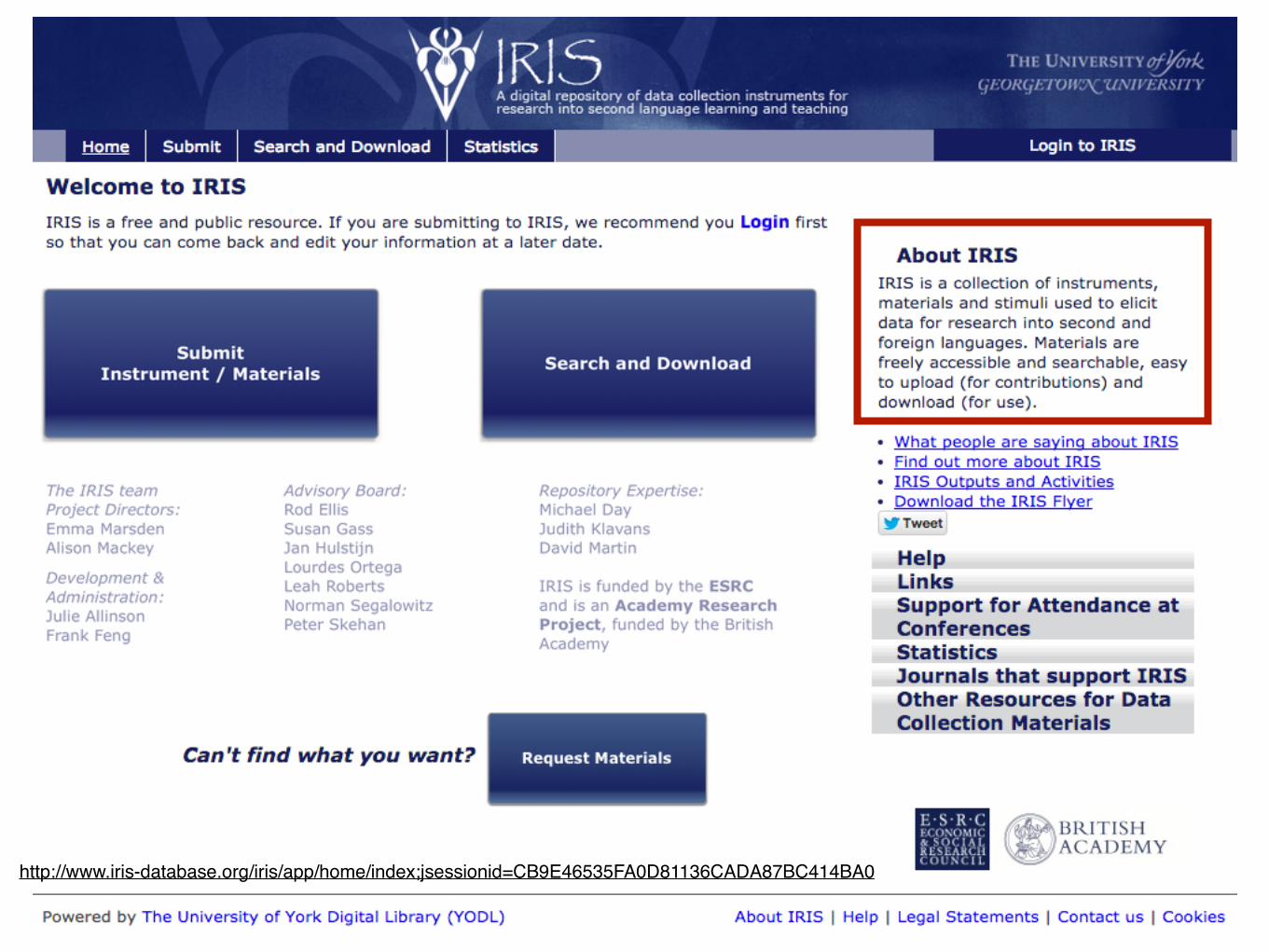
http://www.iris-database.org/iris/app/home/index;jsessionid=CB9E46535FA0D81136CADA87BC414BA0

https://osf.io/
Open Science Framework
Dataverse Projecthttp://dataverse.org/

「いきなり世界戦や。ワシには無理。」 (C)マグロー大学

まとめ• langtest.jp
-「ハンドブック」の分析確認- Rへの橋渡し
• 統計解析の基礎的知識記述統計,検定,効果量と信頼区間,検定力分析
• 進む「統計改革」と研究のオープン化


Recommended!
LET関西支部メソドロジー研究部会通称「メソ犬」
http://www.mizumot.com/methodology
LET中部支部外国語教育基礎研究部会通称「キソケン」
http://bit.ly/1fYsPsO