Sampling with Mirrored Stein Operators

Jiaxin ShiMicrosoft Research

Cambridge, MAjiaxinshi@microsoft.com

Chang LiuMicrosoft Research

Beijingchang.liu@microsoft.com

Lester MackeyMicrosoft Research

Cambridge, MAlmackey@microsoft.com

Abstract

We introduce a new family of particle evolution samplers suitable for constraineddomains and non-Euclidean geometries. Stein Variational Mirror Descent andMirrored Stein Variational Gradient Descent minimize the Kullback-Leibler (KL)divergence to constrained target distributions by evolving particles in a dual spacedefined by a mirror map. Stein Variational Natural Gradient exploits non-Euclideangeometry to more efficiently minimize the KL divergence to unconstrained targets.We derive these samplers from a new class of mirrored Stein operators and adaptivekernels developed in this work. We demonstrate that these new samplers yieldaccurate approximations to distributions on the simplex, deliver valid confidence in-tervals in post-selection inference, and converge more rapidly than prior methods inlarge-scale unconstrained posterior inference. Finally, we establish the convergenceof our new procedures under verifiable conditions on the target distribution.

1 Introduction

Accurately approximating an unnormalized distribution with a discrete sample is a fundamental chal-lenge in machine learning, probabilistic inference, and Bayesian inference. Particle evolution methodslike Stein variational gradient descent [SVGD, 44] tackle this challenge by applying deterministicupdates to particles using operators based on Stein’s method [60, 26, 51, 45, 13, 27] and reproducingkernels [6] to sequentially minimize Kullback-Leibler (KL) divergence. SVGD has found greatsuccess in approximating unconstrained distributions for probabilistic learning [21, 30, 39] but breaksdown for constrained targets, like distributions on the simplex [53] or the targets of post-selectioninference [62, 40, 63], and fails to exploit informative non-Euclidean geometry [2].

In this work, we derive a family of particle evolution samplers suitable for target distributions withconstrained domains and non-Euclidean geometries. Our development draws inspiration from mirrordescent (MD) [50], a first-order optimization method that generalizes gradient descent with non-Euclidean geometry. To sample from a distribution with constrained support, our method first mapsparticles to a dual space. There, we update particle locations using a new class of mirrored Steinoperators and adaptive reproducing kernels introduced in this work. Finally, the dual particles aremapped back to sample points in the original space, ensuring that all constraints are satisfied. Weillustrate this procedure in Fig. 1. In Sec. 3, we develop two algorithms – Mirrored SVGD (MSVGD)and Stein Variational Mirror Descent (SVMD) – with different updates in the dual space; when only asingle particle is used, MSVGD reduces to gradient ascent on the log dual space density, and SVMDreduces to mirror ascent on the log target density. In addition, by exploiting the connection betweenMD and natural gradient descent [2, 54], we develop a third algorithm – Stein Variational NaturalGradient (SVNG) – that extends SVMD to unconstrained targets with non-Euclidean geometry.

In Sec. 5, we demonstrate the advantages of our algorithms on benchmark simplex-constrainedproblems from the literature, constrained sampling problems in post-selection inference [62, 40, 63],and unconstrained large-scale posterior inference with the Fisher information metric. Finally, weanalyze the convergence of our mirrored algorithms in Sec. 6 and discuss our results in Sec. 7.

Preprint. Under review.

arX

iv:2

106.

1250

6v1

[st

at.M

L]

23

Jun

2021

Θ

∇ψ

∇ψ∗

θtθt+1

ηt

ηt+1

εtEθ∼qt [Mp,ψK(θt, θ)]

Figure 1: Updating particle approximations in constrained domains Θ. Standard updates like SVGD(dashed arrow) can push particles outside of the support. Our mirrored Stein updates in Alg. 1 (solidarrows) preserve the support by updating particles in a dual space and mapping back to Θ.

Related work Our mirrored Stein operators (7) are instances of diffusion Stein operators in thesense of [27], but their specific properties have not been studied, nor have they been used to developsampling algorithms. There is now a large body of work on transferring algorithmic ideas fromoptimization to sampling [see, e.g., 14, 67, 18, 47, 59]. The closest to our work in this space isthe recent marriage of mirror descent and MCMC. For example, Hsieh et al. [34] propose to runLangevin Monte Carlo (LMC, an Euler discretization of the Langevin diffusion) in a mirror space.Zhang et al. [70] analyze the convergence properties of the mirror-Langevin diffusion, Chewi et al.[12] demonstrate its advantages over the Langevin diffusion when using a Newton-type metric, andAhn and Chewi [1] study its discretization for MCMC sampling in constrained domains. Relatedly,Patterson and Teh [53] proposed stochastic Riemannian LMC for sampling on the simplex.

Several modifications of SVGD have been proposed to incorporate geometric information. Rieman-nian SVGD [RSVGD, 42] generalizes SVGD to Riemannian manifolds, but, even with the samemetric tensor, their updates are more complex than ours, do not operate in a mirror space, requirehigher-order kernel derivatives, and reportedly do not perform well when with scalable stochasticestimates of ∇ log p. Stein Variational Newton [SVN, 15, 9] introduces second-order informationinto SVGD. Their algorithm requires an often expensive Hessian computation and need not leadto descent directions, so inexact approximations are employed in practice. Our SVNG can be seenas an instance of matrix SVGD [MatSVGD, 66] with an adaptive time-dependent kernel discussedin Sec. 4.4, a choice that is not explored in [66] and which recovers natural gradient descent whenn = 1 unlike the heuristic kernel constructions of [66]. None of the aforementioned works provideconvergence guarantees, and neither SVN nor matrix SVGD deals with constrained domains.

2 Background

2.1 Mirror descent and non-Euclidean geometry

Standard gradient descent can be viewed as optimizing a local quadratic approximation to the targetfunction f : θt+1 = argminθ∈Θ∇f(θt)

>θ + 12εt‖θ − θt‖22. When Θ ⊆ Rd is constrained, it can be

advantageous to replace ‖ · ‖2 with a function Ψ that reflects the geometry of a problem [50, 5]:

θt+1 = argminθ∈Θ∇f(θt)>θ + 1

εtΨ(θ, θt). (1)

We consider the mirror descent algorithm [50, 5] which chooses Ψ to be the Bregman divergenceinduced by a strictly convex function ψ : Θ→ R∪∞: Ψ(θ, θ′) = ψ(θ)−ψ(θ′)−∇ψ(θ′)>(θ−θ′).When Θ is a (d+ 1)-simplex θ :

∑di=1 θi ≤ 1 and θi ≥ 0 for i ∈ [d], a common choice of ψ is the

negative entropy ψ(θ) =∑d+1i=1 θi log θi, for θd+1 , 1−∑d

i=1 θd. The solution of (1) is given by

θt+1 = ∇ψ∗(∇ψ(θt)− εt∇f(θt)), (2)

where ψ∗(η) , supθ∈Θ η>θ − ψ(θ) is the convex conjugate of ψ and ∇ψ is a bijection from Θ to

dom(ψ∗) with inverse map (∇ψ)−1 = ∇ψ∗. We can view the update in (2) as first mapping θt to ηtby∇ψ, applying the update ηt+1 = ηt − εt∇f(θt), and mapping back through θt+1 = ∇ψ∗(ηt+1).

Mirror descent can also be viewed as a discretization of the continuous-time dynamics dηt =−∇f(θt)dt, θt = ∇ψ∗(ηt), which is equivalent to the Riemannian gradient flow

dθt = −∇2ψ(θt)−1∇f(θt)dt, or equivalently, dηt = −∇2ψ∗(ηt)

−1∇ηtf(∇ψ∗(ηt))dt, (3)

2

where ∇2ψ(θ) and ∇2ψ∗(η) are Riemannian metric tensors (see App. A). In information geometry,the discretization of (3) is known as natural gradient descent [2]. There is considerable theoreticaland practical evidence [48] showing that natural gradient works efficiently in learning.

2.2 Mirror-Langevin diffusions

Next we review the (overdamped) Langevin diffusion – a Markov process that underlies SVGDand many recent advances in Stein’s method – along with its recent mirrored generalization. TheLangevin diffusion with equilibrium density p on Rd is a Markov process (θt)t≥0 ⊂ Rd satisfyingthe stochastic differential equation (SDE) dθt = ∇ log p(θt)dt +

√2dBt with (Bt)t≥0 a standard

Brownian motion [7, Sec. 4.5]. The Riemannian Langevin diffusion [53, 69, 46] extends the Langevinto non-Euclidean geometries encoded in a positive definite metric tensor G(θ):

dθt = (G(θt)−1∇ log p(θt) +∇ ·G(θt)

−1)dt+√

2G(θt)−1/2dBt.

1

We show in App. B that the choice G = ∇2ψ yields the recent mirror-Langevin diffusion [70, 12]

θt = ∇ψ∗(ηt), dηt = ∇ log p(θt)dt+√

2∇2ψ(θt)1/2dBt. (4)

3 Stein’s Identity and Mirrored Stein Operators

Stein’s identity [60] is a tool for characterizing a target distribution P using a so-called Stein operator.Hereafter, we assume P has a differentiable density p with convex support Θ ⊆ Rd. A Stein operatorSp takes as input functions g from a Stein set G and outputs mean-zero functions under p:

Ep[(Spg)(θ)] = 0, for all g ∈ G. (5)To identify Stein operators for broad classes of targets p, Gorham and Mackey [26] proposed to buildupon Barbour’s generator method [3]. First, identify a Markov process (θt)t≥0 that has p as theequilibrium density; Gorham and Mackey [26] chose the Langevin diffusion of Sec. 2.2. Next, builda Stein operator based on the (infinitesimal) generator A of the process [52, Def. 7.3.1]:

(Af)(θ) = limt→01t (Ef(θt)− Ef(θ0)) for f : Rd → R,

as the generator outputs mean-zero functions under p under relatively mild conditions; the resultingLangevin Stein operator of [26] is given by

(Spg)(θ) = g(θ)>∇ log p(θ) +∇ · g(θ), (6)where g is a vector-valued function and ∇ · g is its divergence. For an unconstrained domain withEp[‖∇ log p(θ)‖2] <∞, Stein’s identity (5) holds for this operator whenever g ∈ C1 is bounded andLipschitz by [28, proof of Prop. 3]. However, on constrained domains Θ, Stein’s identity fails to holdfor many reasonable inputs g if p is non-vanishing or explosive at the boundary.

Motivated by this deficiency and by a desire to exploit non-Euclidean geometry, we propose analternative mirrored Stein operator,

(Mp,ψg)(θ) = g(θ)>∇2ψ(θ)−1∇ log p(θ) +∇ · (∇2ψ(θ)−1g(θ)), (7)

where ψ is a strictly convex mirror function as in Sec. 2.1 with continuously differentiable∇2ψ−1(θ).We derive this operator from the generator of the mirror-Langevin diffusion (4) in App. C. Thefollowing result, proved in App. F.1, shows that Mp,ψ generates mean-zero functions under pwhenever ∇2ψ−1 suitably cancels the growth of p at the boundary.Proposition 1. Suppose that ∇2ψ(θ)−1∇ log p(θ) and ∇ · ∇2ψ(θ)−1 are p-integrable. Iflimr→∞

∫∂Θr

p(θ)‖∇2ψ(θ)−1nr(θ)‖2dθ = 0 for Θr , θ ∈ Θ : ‖θ‖∞ ≤ r and nr(θ) theoutward unit normal vector to ∂Θr at θ, then Ep[(Mp,ψg)(θ)] = 0 if g ∈ C1 is bounded Lipschitz.

Example 1 (Dirichlet p, Negative entropy ψ). When θ1:d+1 ∼ Dir(α) for α ∈ Rd+1+ , even

the common identity Ep[∇ log p(θ)] = 0 need not hold when some αj ≤ 1. However, whenψ(θ) =

∑d+1j=1 θj log θj , the conditions of Prop. 1 are met for any α as∇2ψ(θ)−1 = diag(θ)− θθ>,∫∂Θp(θ)g(θ)>∇2ψ(θ)−1n(θ)dθ =

∑dj=1

∫θj=0

p(θ)(θ>g(θ)− gj(θ))θjdθ−j+ 1√

d

∫θd+1=0

p(θ)θ>g(θ)θd+1dθ = 0

1A matrix divergence∇ ·G(θ) is the vector obtained by computing the divergence of each row of G(θ).

3

by Ding [16, (4)] for any bounded g and n(θ) the outward unit normal vector to ∂Θ at θ, andlimr→∞

∫∂Θr

p(θ)‖∇2ψ(θ)−1nr(θ)‖2dθ = sup‖g‖∞≤1

∫∂Θp(θ)g(θ)>∇2ψ(θ)−1n(θ)dθ. Remark-

ably, the mirror-Langevin diffusion for our choice of ψ is the Wright-Fisher diffusion [20] whichGan et al. [24] recently used to bound distances to Dirichlet distributions.

4 Sampling with Mirrored Stein Operators

Liu and Wang [44] pioneered the idea of using Stein operators to approximate a target distributionwith particles. Their popular SVGD algorithm deterministically updates a set of n particle locationson each step and relies on the interaction between them to approximately sample from a targetdistribution p. The following theorem summarizes their main findings.Theorem 2 ([44, Thm. 3.1]). Suppose (θt)t≥0 satisfies dθt = gt(θt)dt for bounded Lipschitzgt ∈ C1 : Rd → Rd and that θt has density qt with Eqt [‖∇ log qt(θ)‖2] < ∞. If KL(qt‖p) ,Eqt [log(qt(θ)/p(θ))] exists then, for the Langevin Stein operator Sp (6),

ddtKL(qt‖p) = −Eqt [(Spgt)(θ)]. (8)

To sample from a target distribution p, we aim to find the choice of update direction gt that mostquickly decreases KL(qt‖p) at time t, i.e., we aim to minimize d

dtKL(qt‖p) over a set G of candidatedirections gt. SVGD chooses gt in a reproducing kernel Hilbert space [RKHS, 6] norm ball BHd =g : ‖g‖Hd ≤ 1, where Hd is the product RKHS containing vector-valued functions with eachcomponent in the RKHSH of k. Then the optimal g∗t ∈ BHd that minimizes (8) is

g∗t ∝ g∗qt,k , Eqt [k(θ, ·)∇ log p(θ) +∇θk(θ, ·)] = Eqt [SpKk(·, θ)],where we let Kk(θ, θ′) = k(θ, θ′)I , and SpKk(·, θ) denotes applying Sp to each row of Kk(·, θ).SVGD has found great success in approximating unconstrained target distributions p but breaksdown for constrained targets and fails to exploit non-Euclidean geometry. Our goal is to develop newparticle evolution samplers suitable for constrained domains and non-Euclidean geometries.

4.1 Mirrored dynamics

SVGD encounters two difficulties when faced with a constrained support. First, the SVGD updates canpush the random variable θt outside of its support Θ, rendering all future updates undefined. Second,Stein’s identity (5) often fails to hold for candidate directions in BHd (cf. Ex. 1). When this occurs,SVGD need not converge to p as p is not a stationary point of its dynamics (i.e., d

dtKL(qt‖p)|qt=p 6= 0when qt = p). Inspired by mirror descent [50], we consider the following mirrored dynamics

θt = ∇ψ∗(ηt) for dηt = gt(θt)dt, or, equivalently, dθt = ∇2ψ(θt)−1gt(θt)dt, (9)

where gt : Θ → Rd now represents the update direction in η space. The inverse mirror map ∇ψ∗automatically guarantees that θt belongs to the constrained domain Θ. From Thm. 2 it follows that

ddtKL(qt‖p) = −Eqt [(Mp,ψgt)(θ)], (10)

whereMp,ψ is the mirrored Stein operator (7). In the following sections, we propose three newdeterministic sampling algorithms by seeking the optimal direction gt that minimizes (10) overdifferent function classes. Thm. 3 (proved in App. F.2) forms the basis of our analysis.Theorem 3 (Optimal mirror updates in RKHS). Suppose (θt)t≥0 follows the mirrored dynamics (9).Let HK denote the RKHS of a matrix-valued kernel K : Θ × Θ → Sd×d [49]. Then, the optimaldirection of gt that minimizes (10) in the norm ball BHK , g : ‖g‖HK ≤ 1 is

g∗t ∝ g∗qt,K , Eqt [Mp,ψK(·, θ)], (11)

whereMp,ψK(·, θ) appliesMp,ψ (7) to each row of the matrix-valued function Kθ = K(·, θ).

4.2 Mirrored Stein Variational Gradient Descent

Following the pattern of SVGD, one can choose the matrix-valued K of Thm. 3 to be Kk(θ, θ′) =k(θ, θ′)I , where k is any scalar-valued kernel on Θ. In this case, the resulting update g∗qt,Kk(·) =

Eqt [Mp,ψKk(·, θ)] is equivalent to running SVGD in the dual η space before mapping back to Θ.

4

Algorithm 1 Mirrored Stein Variational Gradient Descent & Stein Variational Mirror Descent

Input: density p on Θ, kernel k, mirror function ψ, particles (θi0)ni=1 ⊂ Θ, step sizes (εt)Tt=1

Init: ηi0 ← ∇ψ(θi0) for i ∈ [n]for t = 0 : T do

if SVMD then Kt ← Kψ,t (14) else Kt ← kI (MSVGD)for i ∈ [n], ηit+1 ← ηit + εt

1n

∑nj=1Mp,ψKt(θ

it, θ

jt ) (forMp,ψKt(·, θ) defined in Thm. 3)

for i ∈ [n], θit+1 ← ∇ψ∗(ηit+1)

return θiT+1ni=1.

Theorem 4 (Mirrored SVGD updates). In the setting of Thm. 3, let kψ(η, η′) =k(∇ψ∗(η),∇ψ∗(η′)), pH(η) = p(∇ψ∗(η)) · |det∇2ψ∗(η)| denote the density of η = ∇ψ(θ)when θ ∼ p, and qt,H(η) denote the density of ηt under the mirrored dynamics (9). If Kk = kI ,

g∗qt,Kk(θt) = Eqt,H [kψ(η, ηt)∇ log pH(η) +∇ηkψ(η, ηt)]. (12)

The proof is in App. F.3. By discretizing the dynamics dηt = g∗qt,Kk(θt)dt and initializing with anyparticle approximation q0 = 1

n

∑ni=1 δθi0 , we obtain Mirrored SVGD (MSVGD), our first algorithm

for sampling in constrained domains. The details are summarized in Alg. 1.

When only a single particle is used (n = 1) and the differentiable input kernel satisfies∇k(θ, θ) = 0,the MSVGD update (12) reduces to gradient descent on − log pH(η). Note however that the modesof the mirrored density pH(η) need not match those of the target density p(θ). Since we are primarilyinterested in the θ-space density, it is natural to ask whether there exists a mirrored dynamics thatreduces to finding the mode of p(θ) in this limiting case. In the next section, we give an answer tothis question by designing an adaptive reproducing kernel that yields a mirror descent-like update.

4.3 Stein Variational Mirror Descent

Our second sampling algorithm for constrained problems is called Stein Variational Mirror De-scent (SVMD). We start by introducing a new matrix-valued kernel that incorporates the metric ∇2ψand evolves with the distribution qt.Definition 1 (Kernels for SVMD). Given a continuous scalar-valued kernel k, consider the Mercerrepresentation2 k(θ, θ′) =

∑i≥1 λiui(θ)ui(θ

′) w.r.t. qt, where ui is an eigenfunction satisfying

Eqt(θ′)[k(θ, θ′)ui(θ′)] = λiui(θ). (13)

For k1/2(θ, θ′) ,∑i≥1 λ

1/2i ui(θ)ui(θ

′), we define the adaptive SVMD kernel at time t,

Kψ,t(θ, θ′) , Eθt∼qt [k1/2(θ, θt)∇2ψ(θt)k

1/2(θt, θ′)]. (14)

By Thm. 3, the optimal update direction for the SVMD kernel ball is g∗qt,Kψ,t = Eqt [Mp,ψKψ,t(·, θ)].We obtain the SVMD algorithm (summarized in Alg. 1) by discretizing dηt = g∗qt,Kψ,t(θt)dt andinitializing with q0 = 1

n

∑ni=1 δθi0 . Because of the discrete representation of qt, Kψ,t takes the form

Kψ,t(θ, θ′) =

∑ni=1

∑nj=1 λ

1/2i λ

1/2j ui(θ)uj(θ

′)Γij , for Γij = 1n

∑n`=1 ui(θ

`t)uj(θ

`t)∇2ψ(θ`t).

Here both λi and ui(θj) can be computed by solving a matrix eigenvalue problem involving theparticle set θini=1: Bvj = nλjvj , where B = (k(θi, θj))ni,j=1 ∈ Rn×n is the Gram matrix ofpairwise kernel evaluations at particle locations, and the i-th element of vj is uj(θi). To compute∇θKψ,t(θ, θ

′), we differentiate both sides of (13) to find that∇uj(θi) = 1λj

∑n`=1 vj`∇θik(θi, θ`).

This technique was used in [58] to estimate gradients of eigenfunctions w.r.t. a continuous q. Fol-lowing their recommendations, we truncate the sum at the J-th largest eigenvalues according to athreshold (τ =

∑Jj=1 λj/

∑nj=1 λj) to ensure numerical stability.

Notably, SVMD differs from MSVGD only in its choice of kernel, but, whenever ∇k(θ, θ) = 0, thischange is sufficient to exactly recover mirror descent when n = 1.

2See App. D for background on Mercer representations in non-compact domains.

5

Proposition 5 (Single-particle SVMD is mirror descent). If n = 1, then one step of SVMD becomes

ηt+1 = ηt + εt(k(θt, θt)∇ log p(θt) +∇k(θt, θt)), θt+1 = ∇ψ∗(ηt+1).

Proof When n = 1, λ1 = k(θt, θt), u1 = 1, and thus Kψ,t(θt, θt) = k(θt, θt)∇2ψ(θt).

4.4 Stein Variational Natural Gradient

The fact that SVMD recovers mirror descent as a special case is not only of relevance in constrainedproblems. We next exploit the connection between MD and natural gradient descent discussedin Sec. 2.1 to design a new sampler – Stein Variational Natural Gradient (SVNG) – that moreefficiently approximates unconstrained targets. The idea is to replace the Hessian ∇2ψ(·) in theSVMD dynamics dθt = ∇2ψ(θt)

−1g∗qt,Kψ,t(θt) with a general metric tensor G(·). The result is theRiemannian gradient flow

dθt = G(θt)−1g∗qt,KG,t(θt)dt with KG,t(θ, θ

′) , Eθt∼qt [k1/2(θ, θt)G(θt)k1/2(θt, θ

′)]. (15)

Given any initial particle approximation q0 = 1n

∑ni=1 δθi0 , we discretize these dynamics to obtain

the unconstrained SVNG sampler of Alg. 2 in the appendix. SVNG can be seen as an instance ofMatSVGD [66] with a new adaptive time-dependent kernel G−1(θ)KG,t(θ, θ

′)G−1(θ′). However,similar to Prop. 5 and unlike the heuristic kernels of [66], SVNG reduces to natural gradient ascent forfinding the mode of p(θ) when n = 1. SVNG is well-suited to Bayesian inference problems wherethe target is a posterior distribution p(θ) ∝ π(θ)π(y|θ). There, the metric tensor G(θ) can be setto the Fisher information matrix Eπ(y|θ)[∇ log π(y|θ)∇ log π(y|θ)>] of the data likelihood π(y|θ).Ample precedent from natural gradient variational inference [33, 38] and Riemannian MCMC [53]suggests that encoding problem geometry in this manner often leads to more rapid convergence.

5 Experiments

We next conduct a series of simulated and real-data experiments to assess (1) distributional approxi-mation on the simplex, (2) frequentist confidence interval construction for (constrained) post-selectioninference, and (3) large-scale posterior inference with non-Euclidean geometry. To compare withstandard SVGD on constrained domains and to prevent its particles from exiting the domain Θ,we introduce a Euclidean projection onto Θ following each SVGD update. See App. E for supple-mentary experimental details and https://github.com/thjashin/mirror-stein-samplersfor Python and R code replicating all experiments.

5.1 Approximation quality on the simplex

0 200 400Number of particle updates, T

0.0

0.5

1.0

1.5

En

ergy

dis

tan

ce

Sparse Dirichlet

Projected SVGD

SVMD

MSVGD, k

MSVGD, k2

0 200 400Number of particle updates, T

0.0

0.1

0.2

0.3

Quadratic

Projected SVGD

SVMD

MSVGD, k

MSVGD, k2

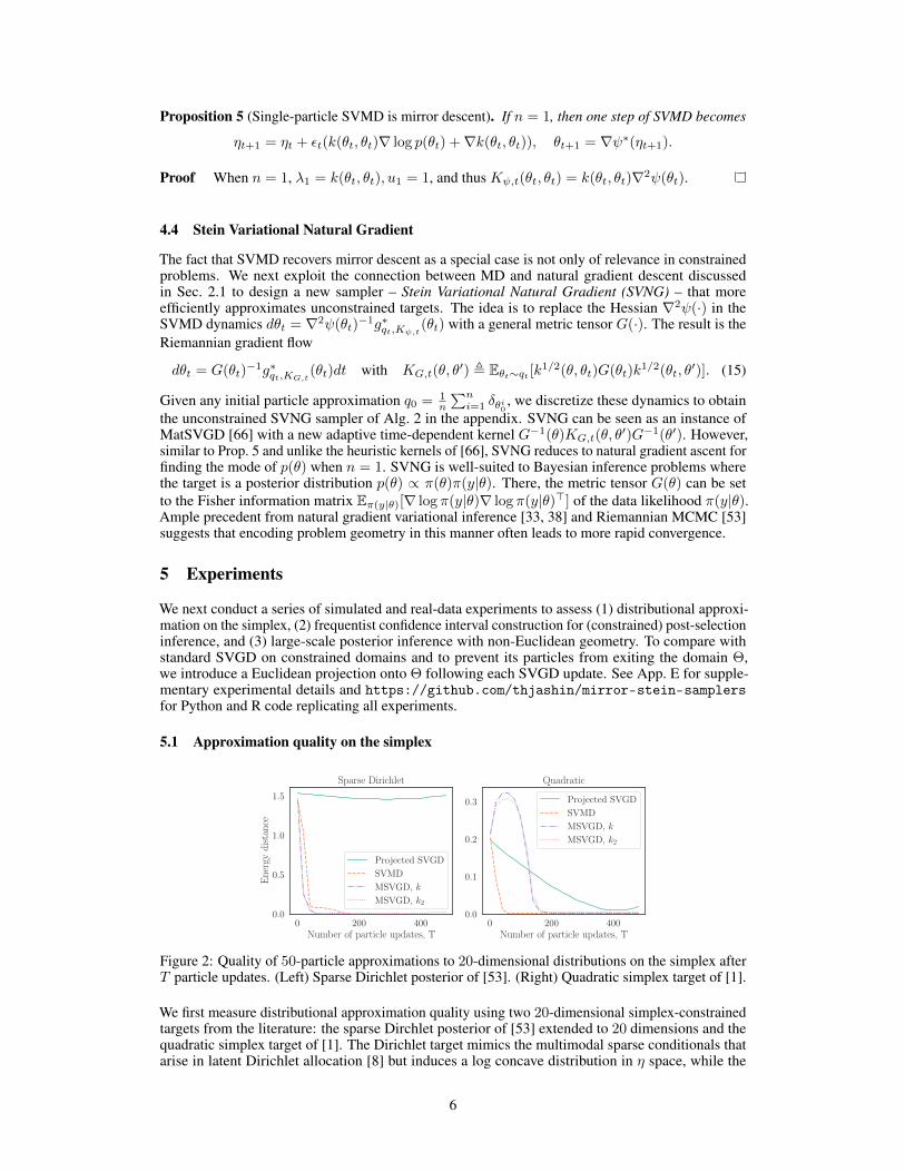
Figure 2: Quality of 50-particle approximations to 20-dimensional distributions on the simplex afterT particle updates. (Left) Sparse Dirichlet posterior of [53]. (Right) Quadratic simplex target of [1].

We first measure distributional approximation quality using two 20-dimensional simplex-constrainedtargets from the literature: the sparse Dirchlet posterior of [53] extended to 20 dimensions and thequadratic simplex target of [1]. The Dirichlet target mimics the multimodal sparse conditionals thatarise in latent Dirichlet allocation [8] but induces a log concave distribution in η space, while the

6

quadratic is log-concave in θ space. In Fig. 2, we compare the quality of MSVGD, SVMD, andprojected SVGD with n = 50 particles and inverse multiquadric base kernel k [27] by computingthe energy distance [61] to a surrogate ground truth sample of size 1000 (drawn i.i.d. or, in thequadratic case, from the No-U-Turn Sampler [32]). We also compare to MSVGD with k2(θ, θ′) =k(∇ψ(θ),∇ψ(θ′)), a choice which corresponds to running SVGD in the dual space with kernel k byThm. 4 and which ensures the convergence of MSVGD to p by the upcoming Thms. 6 to 8.

In the quadratic case, SVMD is favored over MSVGD as it is able to exploit the log-concavity of p(θ).In contrast, for the multimodal sparse Dirichlet with p(θ) unbounded near the boundary, MSVGDconverges slightly more rapidly than SVMD by exploiting the log concave structure in η space. Thisparallels the observation of [34] that LMC in the mirror space outperforms Riemannian LMC forsparse Dirichlet distributions. Projected SVGD fails to converge to the target in both cases and hasparticular difficulty in approximating the sparse Dirichlet target with unbounded density. MSVGDwith k and k2 perform very similarly, but we observe that k yields better approximation quality uponconvergence. Therefore, we employ k in the remaining MSVGD experiments.

5.2 Confidence intervals for post-selection inference

We next apply our algorithms to the constrained sampling problems that arise in post-selectioninference [62, 40]. Specifically, we consider the task of forming valid confidence intervals (CIs) forregression parameters selected using the randomized Lasso [63] with dataX ∈ Rn×p and y ∈ Rn anduser-generated randomness w ∈ Rp from a log-concave distribution with density g. The randomizedLasso returns β ∈ Rp with non-zero coefficients denoted by βE and their signs by sE . It is commonpractice to report least squares CIs for βE by running a linear regression on the selected features E.However, since E is chosen based on the same data, the resulting CIs are often invalid.

Post-selection inference solves this problem by conditioning the inference on the knowledge of Eand sE . To construct valid CIs, it suffices to approximate the selective distribution with supportβE , u−E : sE βE > 0, u−E ∈ [−1, 1]p−|E| and density

g(βE , u−E) ∝ g(X>y −

(X>EXE+εI|E|

X>−EXE

)βE + λ

( sEu−E

)).

In our experiments, we integrate out u−E analytically, following [63], and model |βE | rather thanβE to obtain a log-concave density supported on the positive orthant with mirror function ψ(θ) =∑dj=1(θj log θj − θj). In Fig. 4a we show the example of a 2D selective distribution using samples

drawn by NUTS [32]. We also plot the results by projected SVGD, SVMD, and MSVGD in thisexample. Projected SVGD fails to approximate the target with many samples gathering at thetruncation boundary, while the samples by MSVGD and SVMD closely resemble the truth.

We then compare our methods with the standard norejection MCMC approach of theselectiveInference R package [64] using the example simulation setting described in [57]and a penalty factor 0.7. To generate N total sample points we run MCMC for N iterations afterburn-in or aggregate the particles from N/n independent runs of MSVGD or SVMD with n = 50particles. As N ranges from 1000 to 3000 in Fig. 3a, the MSVGD and SVMD CIs consistentlyyield higher coverage than the standard 90% CIs. This increased coverage is of particular value forsmaller sample sizes, for which the standard CIs tend to undercover. For a much larger sample size ofN = 5000 in Fig. 3b, the SVMD and standard CIs closely track one another across confidence levels,while MSVGD consistently yields longer CIs with high coverage. The higher coverage of MSVGD isonly of value for larger confidence levels at which the other methods begin to undercover.

We next apply our samplers to a post-selection inference task on the HIV-1 drug resistance dataset [55],where we run randomized Lasso [63] to find statistically significant mutations associated with drugresistance using susceptibility data on virus isolates. We take the vitro measurement of log-foldchange under the 3TC drug as response and include mutations that had appeared at least 11 times inthe dataset as regressors. In Fig. 4b we plot the CIs of selected mutations obtained with N = 5000sample points. We see that the invalid unadjusted least squares CIs can lead to premature conclusions,e.g., declaring mutation 215Y significant when there is insufficient support after conditioning on theselection event. In contrast, mutation 184V, which has known association with drug resistance, isdeclared significant by all methods even after post-selection adjustment. The MSVGD and SVMD CIsmostly track those of the standard selectiveInference method, but their conclusions sometimesdiffer: e.g., 62Y is flagged as significant by MSVGD and SVMD but not by selectiveInference.

7

1000 1500 2000 2500 3000Number of sample points, N

0.86

0.88

0.90

0.92

0.94

Act

ual

cove

rage

Standard

MSVGD

SVMD

(a) Nominal coverage: 0.9

0.80 0.85 0.90 0.95 1.00Nominal coverage

0.80

0.85

0.90

0.95

1.00

Act

ual

cove

rage

Standard

MSVGD

SVMD

(b) N = 5000 sample points

Figure 3: Coverage of post-selection CIs across (a) 500 / (b) 200 replications of simulation of [57].

Truth Projected SVGD

SVMD MSVGD

(a)

2.0

2.2

2.4Unadjusted

Standard

SVMD

MSVGD

P41LP62V

P65RP67N

P69iP70R

P83KP151M

P181CP184V

P210WP215Y

−0.2

0.0

0.2

0.4

(b)

Figure 4: (a) Sampling from a 2D selective density; (b) Unadjusted and post-selection CIs for themutations selected by the randomized Lasso as candidates for HIV-1 drug resistance (see Sec. 5.2).

5.3 Large-scale posterior inference with non-Euclidean geometry

Finally, we demonstrate the advantages of exploiting non-Euclidean geometry by recreating thereal-data large-scale Bayesian logistic regression experiment of [44] with 581,012 datapoints andd = 54 feature dimensions. Here, the target p is the posterior distribution over logistic regressionparameters. We adopt the Fisher information metric tensor G, compare 20-particle SVND to SVGDand its prior geometry-aware variants RSVGD [42] and MatSVGD with average and mixture kernels[66], and for all methods use stochastic minibatches of size 256 to scalably approximate each loglikelihood query. In Fig. 5, all geometry-aware methods substantially improve the log predictiveprobability of SVGD.3 SVNG also strongly outperforms RSVGD and converges to its maximum testprobability in half as many steps as MatSVGD (Avg) and more rapidly than MatSVGD (Mixture).

6 Convergence Guarantees

We next turn our attention to the convergence properties of our proposed methods. For Kt and εtas in Alg. 1, let (q∞t , q

∞t,H) represent the distributions of the mirrored Stein updates (θt, ηt) when

θ0 ∼ q∞0 and ηt+1 = ηt + εtg∗qt,Kt

(θt) for t ≥ 0. Our first result, proved in App. F.4, shows that ifthe Alg. 1 initialization qn0,H = 1

n

∑ni=1 δηi0 converges in Wasserstein distance to a distribution q∞0,H

as n→∞, then, on each round t > 0, the output of Alg. 1, qnt = 1n

∑ni=1 δθit , converges to q∞t .

3Notably, on the same dataset, SVGD was shown to outperform preconditioned stochastic gradient Langevindynamics [41], a leading MCMC method imbued with geometric information [66].

8

0 500 1000 1500 2000 2500 3000Number of particle updates, T

−0.58

−0.57

−0.56

−0.55

−0.54

−0.53

−0.52

−0.51

Tes

tlo

gp

red

icti

vep

rob

abili

ty

SVGD

SVNG

RSVGD

0 100 200 300 400Number of particle updates, T

−0.550

−0.545

−0.540

−0.535

−0.530

−0.525

−0.520

−0.515

Tes

tlo

gp

red

icti

vep

rob

abili

ty

SVNG

Matrix SVGD (Avg)

Matrix SVGD (Mixture)

0 50 100 150 200 250 300 350 400Number of particle updates, T

0.0

2.5

5.0

7.5

10.0

12.5

15.0

17.5

Tim

e(s

)

SVNG

Matrix SVGD (Avg)

Matrix SVGD (Mixture)

Figure 5: Value of non-Euclidean geometry in large-scale Bayesian logistic regression.

Theorem 6 (Convergence of mirrored updates as n → ∞). Suppose Alg. 1 is initialized withqn0,H = 1

n

∑ni=1 δηi0 satisfying W1(qn0,H , q

∞0,H)→ 0 for W1 the L1 Wasserstein distance. Define the

η-induced kernel K∇ψ∗,t(η, η′) , Kt(∇ψ∗(η),∇ψ∗(η′)). If, for some c1, c2 > 0,

‖∇(K∇ψ∗,t(·, η)∇ log pH(η) +∇ ·K∇ψ∗,t(·, η))‖op ≤ c1(1 + ‖η‖2),

‖∇(K∇ψ∗,t(η′, ·)∇ log pH(·) +∇ ·K∇ψ∗,t(η′, ·))‖op ≤ c2(1 + ‖η′‖2),

then, W1(qnt,H , q∞t,H)→ 0 and qnt ⇒ q∞t for each round t.

Remark The pre-conditions hold, for example, whenever ∇ log pH is Lipschitz, ψ is stronglyconvex, and Kt = kI for k bounded with bounded derivatives.

Given a mirrored Stein operator (7), an arbitrary Stein set G, and an arbitrary matrix-valued kernel Kwe define the mirrored Stein discrepancy and mirrored kernel Stein discrepancy

MSD(q, p,G) , supg∈G Eq[(Mp,ψg)(θ)] and MKSDK(q, p) , MSD(q, p,BHK ). (16)

The former is an example of a diffusion Stein discrepancy [28] and the latter an example of a diffusionkernel Stein discrepancy [4]. Since the MKSD optimization problem (16) matches that in Thm. 3,we have that MKSDK(q, p) = ‖g∗q,K‖HK . Our next result, proved in App. F.5, shows that theinfinite-particle mirrored Stein updates reduce the KL divergence to p whenever the step size issufficiently small and drive MKSD to 0 if, for example, εt = Ω(MKSDKt(q

∞t , p)

α) for any α > 0.

Theorem 7 (Infinite-particle mirrored Stein updates decrease KL and MKSD). Assume κ1 ,supθ‖Kt(θ, θ)‖op < ∞, and κ2 ,

∑di=1 supθ ‖∇2

i,d+iKt(θ, θ)‖op < ∞, ∇ log pH is L-Lipschitz,and ψ is α-strongly convex. If εt < 1/(‖∇ηtg∗q∞t ,Kt(θt) +∇ηtg∗q∞t ,Kt(θt)

>‖op), then

KL(q∞t+1‖p)− KL(q∞t ‖p) ≤ −(εt −

(Lκ1

2 + 2κ2

α2

)ε2t)MKSDKt(q

∞t , p)

2.

Our last result, proved in App. F.6, shows that q∞t ⇒ p if MKSDKk(q∞t , p)→ 0. Hence, by Thms. 6and 7, n-particle MSVGD converges weakly to p if εt decays at a suitable rate.Theorem 8 (MKSDKk determines weak convergence). Assume pH is distantly dissipative [19] with∇ log pH Lipschitz, ψ is strictly convex with continuous∇ψ∗, and k(θ, θ′) = κ(∇ψ(θ),∇ψ(θ′)) forκ(x, y) = (c2 + ‖x− y‖22)β with β ∈ (−1, 0). Then, q∞t ⇒ p if MKSDKk(q∞t , p)→ 0.

Remark The pre-conditions hold, for example, for any Dirichlet target with negative entropy ψ.

7 Discussion

This paper introduced the mirrored Stein operator along with three new particle evolution algorithmsfor sampling with constrained domains and non-Euclidean geometries. The first algorithm MSVGDperforms SVGD updates in a mirrored space before mapping to the target domain. The other twoalgorithms are different discretizations of the same continuous dynamics for exploiting non-Euclideangeometry. SVMD is a multi-particle generalization of mirror descent for constrained domains, whileSVNG is designed for unconstrained problems with informative metric tensors. We do not anticipatenegative societal impact from this work, but we highlight three limitations. First, like SVGD, ourMSVGD require n2 time per update, and parallelism or low-rank kernel approximation may be

9

needed to reduce this complexity. Second, SVMD and SVNG are more costly than MSVGD due tothe adaptive kernel construction. Third, we leave open the question of convergence when stochasticgradient estimates are employed, but we suspect the results of [29, Thm. 7] can be extended to oursetting. In the future, we hope to deploy our mirrored Stein operators for other inferential taskson constrained domains including sample quality measurement [26, 27, 28, 35], goodness-of-fittesting [13, 45, 36], graphical model inference [71, 65], parameter estimation [4], thinning [56], andde novo sampling [10, 11, 23].

References[1] Kwangjun Ahn and Sinho Chewi. Efficient constrained sampling via the mirror-Langevin algorithm. arXiv

preprint arXiv:2010.16212, 2020.

[2] Shun-Ichi Amari. Natural gradient works efficiently in learning. Neural Computation, 10(2):251–276,1998.

[3] Andrew D Barbour. Stein’s method and Poisson process convergence. Journal of Applied Probability,pages 175–184, 1988.

[4] Alessandro Barp, Francois-Xavier Briol, Andrew Duncan, Mark Girolami, and Lester Mackey. MinimumStein discrepancy estimators. In Advances in Neural Information Processing Systems, pages 12964–12976,2019.

[5] Amir Beck and Marc Teboulle. Mirror descent and nonlinear projected subgradient methods for convexoptimization. Operations Research Letters, 31(3):167–175, 2003.

[6] Alain Berlinet and Christine Thomas-Agnan. Reproducing kernel Hilbert spaces in probability andstatistics. Springer Science & Business Media, 2011.

[7] Rabi N Bhattacharya and Edward C Waymire. Stochastic processes with applications. SIAM, 2009.

[8] David M Blei, Andrew Y Ng, and Michael I Jordan. Latent Dirichlet allocation. Journal of MachineLearning Research, 3:993–1022, 2003.

[9] Peng Chen, Keyi Wu, Joshua Chen, Tom O'Leary-Roseberry, and Omar Ghattas. Projected Stein variationalNewton: A fast and scalable Bayesian inference method in high dimensions. In Advances in NeuralInformation Processing Systems, volume 32, 2019.

[10] Wilson Ye Chen, Lester Mackey, Jackson Gorham, François-Xavier Briol, and Chris Oates. Stein points.In International Conference on Machine Learning, pages 844–853, 2018.

[11] Wilson Ye Chen, Alessandro Barp, François-Xavier Briol, Jackson Gorham, Mark Girolami, Lester Mackey,and Chris Oates. Stein point Markov chain Monte Carlo. In International Conference on Machine Learning,pages 1011–1021, 2019.

[12] Sinho Chewi, Thibaut Le Gouic, Chen Lu, Tyler Maunu, Philippe Rigollet, and Austin Stromme. Exponen-tial ergodicity of mirror-Langevin diffusions. arXiv preprint arXiv:2005.09669, 2020.

[13] Kacper Chwialkowski, Heiko Strathmann, and Arthur Gretton. A kernel test of goodness of fit. InInternational Conference on Machine Learning, pages 2606–2615, 2016.

[14] Arnak Dalalyan. Further and stronger analogy between sampling and optimization: Langevin Monte Carloand gradient descent. In Conference on Learning Theory, pages 678–689, 2017.

[15] Gianluca Detommaso, Tiangang Cui, Youssef Marzouk, Alessio Spantini, and Robert Scheichl. A Steinvariational Newton method. In Advances in Neural Information Processing Systems, volume 31, pages9187–9197, 2018.

[16] Yiren Ding. The law of cosines for an n-dimensional simplex. International Journal of MathematicalEducation in Science and Technology, 39(3):407–410, 2008.

[17] John Duchi, Elad Hazan, and Yoram Singer. Adaptive subgradient methods for online learning andstochastic optimization. Journal of Machine Learning Research, 12(7), 2011.

[18] Alain Durmus, Eric Moulines, and Marcelo Pereyra. Efficient Bayesian computation by proximal Markovchain Monte Carlo: when Langevin meets Moreau. SIAM Journal on Imaging Sciences, 11(1):473–506,2018.

[19] Andreas Eberle. Reflection couplings and contraction rates for diffusions. Probability Theory and RelatedFields, 166(3):851–886, 2016.

[20] Stewart N Ethier. A class of degenerate diffusion processes occurring in population genetics. Communica-tions on Pure and Applied Mathematics, 29(5):483–493, 1976.

[21] Yihao Feng, Dilin Wang, and Qiang Liu. Learning to draw samples with amortized Stein variationalgradient descent. Uncertainty in Artificial Intelligence, 2017.

10

[22] JC Ferreira and VA Menegatto. Eigenvalues of integral operators defined by smooth positive definitekernels. Integral Equations and Operator Theory, 64(1):61–81, 2009.

[23] Futoshi Futami, Zhenghang Cui, Issei Sato, and Masashi Sugiyama. Bayesian posterior approximation viagreedy particle optimization. In Proceedings of the AAAI Conference on Artificial Intelligence, volume 33,pages 3606–3613, 2019.

[24] Han L Gan, Adrian Röllin, and Nathan Ross. Dirichlet approximation of equilibrium distributions inCannings models with mutation. Advances in Applied Probability, 49(3):927–959, 2017.

[25] Damien Garreau, Wittawat Jitkrittum, and Motonobu Kanagawa. Large sample analysis of the medianheuristic. arXiv preprint arXiv:1707.07269, 2017.

[26] Jackson Gorham and Lester Mackey. Measuring sample quality with Stein’s method. In Advances inNeural Information Processing Systems, pages 226–234, 2015.

[27] Jackson Gorham and Lester Mackey. Measuring sample quality with kernels. In International Conferenceon Machine Learning, pages 1292–1301, 2017.

[28] Jackson Gorham, Andrew B Duncan, Sebastian J Vollmer, and Lester Mackey. Measuring sample qualitywith diffusions. The Annals of Applied Probability, 29(5):2884–2928, 2019.

[29] Jackson Gorham, Anant Raj, and Lester Mackey. Stochastic stein discrepancies. arXiv preprintarXiv:2007.02857, 2020.

[30] Tuomas Haarnoja, Haoran Tang, Pieter Abbeel, and Sergey Levine. Reinforcement learning with deepenergy-based policies. In International Conference on Machine Learning, pages 1352–1361, 2017.

[31] Geoffrey Hinton, Nitish Srivastava, and Kevin Swersky. Neural networks for machine learning lecture 6a:overview of mini-batch gradient descent. 2012.

[32] Matthew D Hoffman and Andrew Gelman. The No-U-Turn sampler: adaptively setting path lengths inHamiltonian Monte Carlo. Journal of Machine Learning Research, 15(1):1593–1623, 2014.

[33] Matthew D Hoffman, David M Blei, Chong Wang, and John Paisley. Stochastic variational inference.Journal of Machine Learning Research, 14(5), 2013.

[34] Ya-Ping Hsieh, Ali Kavis, Paul Rolland, and Volkan Cevher. Mirrored Langevin dynamics. In Advances inNeural Information Processing Systems, pages 2878–2887, 2018.

[35] Jonathan Huggins and Lester Mackey. Random feature Stein discrepancies. In S. Bengio, H. Wallach,H. Larochelle, K. Grauman, N. Cesa-Bianchi, and R. Garnett, editors, Advances in Neural InformationProcessing Systems, pages 1903–1913. 2018.

[36] Wittawat Jitkrittum, Wenkai Xu, Zoltán Szabó, K. Fukumizu, and A. Gretton. A Linear-Time KernelGoodness-of-Fit Test. In Advances in Neural Information Processing Systems, 2017.

[37] Sham Kakade, Shai Shalev-Shwartz, Ambuj Tewari, et al. On the duality of strong convexity and strongsmoothness: Learning applications and matrix regularization. Unpublished Manuscript, 2(1), 2009.

[38] Mohammad Emtiyaz Khan and Didrik Nielsen. Fast yet simple natural-gradient descent for variationalinference in complex models. In 2018 International Symposium on Information Theory and Its Applications(ISITA), pages 31–35. IEEE, 2018.

[39] Taesup Kim, Jaesik Yoon, Ousmane Dia, Sungwoong Kim, Yoshua Bengio, and Sungjin Ahn. Bayesianmodel-agnostic meta-learning. Advances in Neural Information Processing Systems, 2018.

[40] Jason D Lee, Dennis L Sun, Yuekai Sun, and Jonathan E Taylor. Exact post-selection inference, withapplication to the lasso. Annals of Statistics, 44(3):907–927, 2016.

[41] Chunyuan Li, Changyou Chen, David Carlson, and Lawrence Carin. Preconditioned stochastic gradientlangevin dynamics for deep neural networks. In Proceedings of the AAAI Conference on ArtificialIntelligence, volume 30, 2016.

[42] Chang Liu and Jun Zhu. Riemannian Stein variational gradient descent for Bayesian inference. InProceedings of the AAAI Conference on Artificial Intelligence, pages 3627–3634, 2018.

[43] Qiang Liu. Stein variational gradient descent as gradient flow. In Advances in Neural InformationProcessing Systems, pages 3115–3123, 2017.

[44] Qiang Liu and Dilin Wang. Stein variational gradient descent: A general purpose Bayesian inferencealgorithm. Advances in Neural Information Processing Systems, 29:2378–2386, 2016.

[45] Qiang Liu, Jason Lee, and Michael Jordan. A kernelized Stein discrepancy for goodness-of-fit tests. InInternational Conference on Machine Learning, pages 276–284, 2016.

[46] Yi-An Ma, Tianqi Chen, and Emily Fox. A complete recipe for stochastic gradient MCMC. In Advancesin Neural Information Processing Systems, pages 2917–2925, 2015.

11

[47] Yi-An Ma, Niladri Chatterji, Xiang Cheng, Nicolas Flammarion, Peter Bartlett, and Michael I Jordan. Isthere an analog of Nesterov acceleration for MCMC? arXiv preprint arXiv:1902.00996, 2019.

[48] James Martens. New insights and perspectives on the natural gradient method. arXiv preprintarXiv:1412.1193, 2014.

[49] Charles A Micchelli and Massimiliano Pontil. On learning vector-valued functions. Neural Computation,17(1):177–204, 2005.

[50] Arkadij Semenovic Nemirovskij and David Borisovich Yudin. Problem complexity and method efficiencyin optimization. 1983.

[51] Chris J Oates, Mark Girolami, and Nicolas Chopin. Control functionals for Monte Carlo integration.Journal of the Royal Statistical Society: Series B (Methodological), 79(3):695–718, 2017.

[52] Bernt Øksendal. Stochastic Differential Equations: An Introduction with Applications. Springer Science &Business Media, 2003.

[53] Sam Patterson and Yee Whye Teh. Stochastic gradient Riemannian Langevin dynamics on the probabilitysimplex. In Advances in Neural Information Processing Systems, pages 3102–3110, 2013.

[54] Garvesh Raskutti and Sayan Mukherjee. The information geometry of mirror descent. IEEE Transactionson Information Theory, 61(3):1451–1457, 2015.

[55] Soo-Yon Rhee, Jonathan Taylor, Gauhar Wadhera, Asa Ben-Hur, Douglas L Brutlag, and Robert W Shafer.Genotypic predictors of human immunodeficiency virus type 1 drug resistance. Proceedings of the NationalAcademy of Sciences, 103(46):17355–17360, 2006.

[56] Marina Riabiz, Wilson Chen, Jon Cockayne, Pawel Swietach, Steven A Niederer, Lester Mackey, ChrisOates, et al. Optimal thinning of MCMC output. arXiv preprint arXiv:2005.03952, 2020.

[57] Amir Sepehri and Jelena Markovic. Non-reversible, tuning-and rejection-free Markov chain Monte Carlovia iterated random functions. arXiv preprint arXiv:1711.07177, 2017.

[58] Jiaxin Shi, Shengyang Sun, and Jun Zhu. A spectral approach to gradient estimation for implicit distribu-tions. In International Conference on Machine Learning, pages 4644–4653, 2018.

[59] Umut Simsekli, Roland Badeau, Taylan Cemgil, and Gaël Richard. Stochastic quasi-Newton LangevinMonte Carlo. In International Conference on Machine Learning, pages 642–651, 2016.

[60] Charles Stein. A bound for the error in the normal approximation to the distribution of a sum of dependentrandom variables. In Proceedings of the Sixth Berkeley Symposium on Mathematical Statistics andProbability, Volume 2: Probability Theory. The Regents of the University of California, 1972.

[61] Gábor J Székely and Maria L Rizzo. Energy statistics: A class of statistics based on distances. Journal ofStatistical Planning and Inference, 143(8):1249–1272, 2013.

[62] Jonathan Taylor and Robert J Tibshirani. Statistical learning and selective inference. Proceedings of theNational Academy of Sciences, 112(25):7629–7634, 2015.

[63] Xiaoying Tian and Jonathan Taylor. Selective inference with a randomized response. The Annals ofStatistics, 46(2):679–710, 2018.

[64] Ryan Tibshirani, Rob Tibshirani, Jonatha Taylor, Joshua Loftus, Stephen Reid, and Jelena Markovic.selectiveInference: Tools for Post-Selection Inference, 2019. URL https://CRAN.R-project.org/package=selectiveInference. R package version 1.2.5.

[65] Dilin Wang, Zhe Zeng, and Qiang Liu. Stein variational message passing for continuous graphical models.In International Conference on Machine Learning, pages 5219–5227, 2018.

[66] Dilin Wang, Ziyang Tang, Chandrajit Bajaj, and Qiang Liu. Stein variational gradient descent withmatrix-valued kernels. In Advances in Neural Information Processing Systems, pages 7836–7846, 2019.

[67] Max Welling and Yee W Teh. Bayesian learning via stochastic gradient Langevin dynamics. In InternationalConference on Machine Learning, pages 681–688, 2011.

[68] Edwin B Wilson. Probable inference, the law of succession, and statistical inference. Journal of theAmerican Statistical Association, 22(158):209–212, 1927.

[69] Tatiana Xifara, Chris Sherlock, Samuel Livingstone, Simon Byrne, and Mark Girolami. Langevin diffusionsand the Metropolis-adjusted Langevin algorithm. Statistics & Probability Letters, 91:14–19, 2014.

[70] Kelvin Shuangjian Zhang, Gabriel Peyré, Jalal Fadili, and Marcelo Pereyra. Wasserstein control of mirrorLangevin Monte Carlo. arXiv preprint arXiv:2002.04363, 2020.

[71] Jingwei Zhuo, Chang Liu, Jiaxin Shi, Jun Zhu, Ning Chen, and Bo Zhang. Message passing Steinvariational gradient descent. In International Conference on Machine Learning, pages 6018–6027, 2018.

12

Algorithm 2 Stein Variational Natural Gradient (SVNG)

Input: density p(θ) on Rd, kernel k, metric tensor G(θ), particles (θi0)ni=1, step sizes (εt)Tt=1

for t = 0 : T dofor i ∈ [n], θit+1 ← θit + εtG(θit)

−1g∗G,t(θit), where

g∗G,t(θ) = 1n

∑nj=1[KG,t(θ, θ

jt )G(θjt )

−1∇ log p(θjt )+∇θjt ·(KG,t(θ, θjt )G(θjt )

−1)] (see (15))

return xiT+1ni=1.

A Mirror Descent, Riemannian Gradient Flow, and Natural Gradient

The equivalence between the mirror flow dηt = −∇f(θt)dt, θt = ∇ψ∗(ηt)dt and the Riemanniangradient flow in (3) is a direct result of the chain rule:

dθtdt

= −∇ηtθtdηtdt

= −(∇θtηt)−1 dηtdt

= −∇2ψ(θt)−1∇f(θt), (17)

dηtdt

= −∇f(θt) = −∇θtηt∇ηtf(∇ψ∗(ηt)) = −∇2ψ∗(ηt)−1∇ηtf(∇ψ∗(ηt)). (18)

Depending on discretizing (17) or (18), there are two natural gradient descent (NGD) updates thatcan arise from the same gradient flow:

NGD (a): θt+1 = θt − εt∇2ψ(θt)−1∇f(θt),

NGD (b): ηt+1 = ηt − εt∇2ψ∗(ηt)−1∇ηtf(∇ψ∗(ηt)).

With finite step sizes εt, their updates need not be the same and can lead to different optimizationpaths. Since ∇f(θt) = ∇2ψ∗(ηt)

−1∇ηtf(∇ψ∗(ηt)), NGD (b) is equivalent to the dual-spaceupdate by mirror descent. This relationship was pointed out in [54] and has been used for developingnatural gradient variational inference algorithms [38]. We emphasize, however, our SVNG algorithmdeveloped in Sec. 4.4 corresponds to the discretization in the primal space as in NGD (a). Therefore,it does not require an explicit dual space, and allows replacing∇2ψ with more general informationmetric tensors.

B Riemannian Langevin Diffusions and Mirror-Langevin Diffusions

Zhang et al. [70] pointed out (4) is a particular case of the Riemannian LD. However, they did notgive an explicit derivation. The Riemannian LD [53, 69, 46] with∇2ψ(·) as metric tensor is

dθt = (∇2ψ(θt)−1∇ log p(θt) +∇ · ∇2ψ(θt)

−1)dt+√

2∇2ψ(θt)−1/2dBt. (19)

To see the connection with mirror-Langevin diffusion, we would like to obtain the SDE that describesthe evolution of ηt = ∇ψ(θt) under the diffusion. This requires the following theorem that providesthe analog of the “chain rule” in SDEs.Theorem 9 (Itô formula [52, Thm 4.2.1]). Let (xt)t≥0 be an Itô process in X ⊂ Rd satisfyingdxt = b(xt)dt+ σ(xt)dBt. Let f(x) ∈ C2 : Rd → Rd′ . Then yt = f(xt) is again an Itô process,and its i-th dimension satisfies

dyt,i = (∇fi(xt)>b(xt) +1

2Tr(∇2fi(xt)σ(xt)σ(xt)

>)dt+∇fi(xt)>σ(xt)dBt.

Substituting∇ψ for f in Thm. 9, we have the SDE of ηt = ∇ψ(θt) as

dηt = (∇ log p(θt) +∇2ψ(θt)∇ · ∇2ψ(θt)−1 + h(θt))dt+∇2ψ(θt)

1/2dBt,

where h(θt)i = Tr(∇2θt

(∇θt,iψ(θt))∇2ψ(θt)−1). Moreover, we have

[∇2ψ(θt)∇ · ∇2ψ(θt)−1]i + Tr(∇2

θt(∇θt,iψ(θt))∇2ψ(θt)−1)

=

d∑`=1

d∑j=1

∇2ψ(θt)ij∇θt,` [∇2ψ(θt)−1]j` +

d∑`=1

d∑j=1

∇θt,`∇2ψ(θt)ij [∇2ψ(θt)−1]j`

=

d∑`=1

∇θt,`

d∑j=1

∇2ψ(θt)ij [∇2ψ(θt)−1]j`

=

d∑`=1

∇θt,`Ii` = 0.

13

Therefore, the ηt diffusion is described by the SDE:

dηt = ∇ log p(θt)dt+∇2ψ(θt)1/2dBt, θt = ∇ψ∗(ηt).

C Derivation of the Mirrored Stein Operator

The following theorem characterizes the generator of processes described by the SDEs.Theorem 10 (Generator of Itô diffusion [52, Thm 7.3.3]). Let (xt)t≥0 be the Itô diffusion in X ⊆ Rd

satisfying dxt = b(xt)dt+σ(xt)dBt. For any f ∈ C2c (X ), the (infinitesimal) generatorA of (xt)t≥0

is

(Af)(x) = b(x)>∇f(x) + 12 Tr(σ(x)σ(x)>∇2f(x)).

According to Thm. 10, the generator of the mirror-Langevin diffusion described by (19) is

(Ap,ψf)(θ) = (∇2ψ(θ)−1∇ log p(θ) +∇ · ∇2ψ(θ)−1)>∇f(θ) + Tr(∇2ψ(θ)−1∇2f(θ))

= ∇f(θ)>∇2ψ(θ)−1∇ log p(θ) +∇ · (∇2ψ(θ)−1∇f(θ)).

Now substituting g(θ) for ∇f(θ), we obtain the associated mirrored Stein operator:

(Mp,ψg)(θ) = g(θ)>∇2ψ(θ)−1∇ log p(θ) +∇ · (∇2ψ(θ)−1g(θ)).

D Background on Reproducing Kernel Hilbert Spaces

Let H be a Hilbert space of functions defined on X and taking their values in R. We say k is areproducing kernel (or kernel) ofH if ∀x ∈ X , k(x, ·) ∈ H and ∀f ∈ H, 〈f, k(x, ·)〉H = f(x). H iscalled a reproducing kernel Hilbert space (RKHS) if it has a kernel. Kernels are positive definite (p.d.)functions, which means that matrices with the form (k(xi, xj))ij are positive semidefinite. For anyp.d. function k, there is a unique RKHS with k as the reproducing kernel, which can be constructedby the completion of ∑n

i=1 aik(xi, ·), xi ∈ X , ai ∈ R, i ∈ N.Now we assume X is a metric space, k is a bounded continuous kernel with the RKHSH, and ν is apositive measure on X . L2(ν) denote the space of all square-integrable functions w.r.t. ν. Then thekernel integral operator Tk : L2(ν)→ L2(ν) defined by

Tkg =

∫Xg(x)k(x, ·)dν

is compact and self-adjoint. Therefore, according to the spectral theorem, there exists an at mostcountable set of positive eigenvalues λjj∈J ⊂ R with λ1 ≥ λ2 ≥ . . . converging to zero andorthonormal eigenfunctions ujj∈J such that

Tkuj = λjuj ,

and k has the representation k(x, x′) =∑j∈J λjuj(x)uj(x

′) (Mercer’s theorem on non-compactdomains), where the convergence of the sum is absolute and uniform on compact subsets of X ×X [22].

E Supplementary Experimental Details and Additional Results

In this section, we report supplementary details and additional results from the experiments of Sec. 5.In Secs. 5.1 and 5.2, we use the inverse multiquadric input kernel k(θ, θ′) = (1 + ‖θ − θ′‖22/`2)−1/2

due to its convergence control properties [27]. In the unconstrained experiments of Sec. 5.3, weuse the Gaussian kernel k(θ, θ′) = exp(−‖θ − θ′‖22/`2) for consistency with past work. Thebandwidth ` is determined by the median heuristic [25]. We select τ from 0.98, 0.99 for all SVMDexperiments. For unconstrained targets, we report, for each method, results from the best fixed stepsize ε ∈ 0.01, 0.05, 0.1, 0.5, 1 selected on a separate validation set. For constrained targets, weselect step sizes adaptively to accommodate rapid density growth near the boundary; specifically, weuse RMSProp [31], an extension of the AdaGrad algorithm [17] used in [44], and report performancewith the best learning rate. Results were recorded on an Intel(R) Xeon(R) CPU E5-2690 v4 @2.60GHz and an NVIDIA Tesla P100 PCIe 16GB.

14

E.1 Approximation quality on the simplex

The sparse Dirichlet posterior of [53] extended to 20 dimensions features a sparse, symmetricDir(α) prior with αk = 0.1 for k ∈ 1, . . . , 20 and sparse count data n1 = 90, n2 = n3 =5, nj = 0 (j > 3), modeled via a multinomial likelihood. The quadratic target satisfies log p(θ) =− 1

2σ2 θ>Aθ + const, where we slightly modify the target density of [1] to make it less flat by

introducing a scale parameter σ = 0.01. A ∈ R19×19 is a positive definite matrix generated bynormalizing products of random matrices with i.i.d. elements drawn from Unif[−1, 1].

We initialize all methods with i.i.d samples from Dirichlet(5) to prevent any of the initial particlesbeing too close to the boundary. For each method and each learning rate we apply 500 particle updates.For SVMD we set τ = 0.98. We search the base learning rates of RMSProp in 0.1, 0.01, 0.001 forSVMD and MSVGD. Since projected SVGD applies updates in the θ space, the appropriate learningrate range is smaller than those of SVMD and MSVGD. There we search the base learning rate ofRMSProp in 0.01, 0.001, 0.0001. For all methods the results under each base learning rate areplotted in Fig. 6.

0 200 400Number of particle updates, T

0.0

0.5

1.0

1.5

En

ergy

dis

tan

ce

Projected SVGD

LR=0.01

LR=0.001

LR=0.0001

0 200 400Number of particle updates, T

0.0

0.5

1.0

1.5

SVMD

LR=0.1

LR=0.01

LR=0.001

0 200 400Number of particle updates, T

0.0

0.5

1.0

1.5

MSVGD, k

LR=0.1

LR=0.01

LR=0.001

0 200 400Number of particle updates, T

0.0

0.5

1.0

1.5

MSVGD, k2

LR=0.1

LR=0.01

LR=0.001

Figure 6: Sampling from a Dirichlet target on a 20-simplex. We plot the energy distance to a groundtruth sample of size 1000.

0 200 400Number of particle updates, T

0.0

0.1

0.2

0.3

En

ergy

dis

tan

ce

Projected SVGD

LR=0.01

LR=0.001

LR=0.0001

0 200 400Number of particle updates, T

0.0

0.1

0.2

0.3

SVMD

LR=0.1

LR=0.01

LR=0.001

0 200 400Number of particle updates, T

0.0

0.1

0.2

0.3

MSVGD, k

LR=0.1

LR=0.01

LR=0.001

0 200 400Number of particle updates, T

0.0

0.1

0.2

0.3

MSVGD, k2

LR=0.1

LR=0.01

LR=0.001

Figure 7: Sampling from a quadratic target on a 20-simplex. We plot the energy distance to a groundtruth sample of size 1000 drawn by NUTS [32].

E.2 Confidence intervals for post-selection inference

Given a dataset X ∈ Rn×p, y ∈ Rn, the randomized Lasso [63] solves the following problem:

argminβ∈Rp12‖y −Xβ‖

22 + λ‖β‖1 − w>β + ε

2‖β‖22, w ∼ G.

where G is a user-specified log-concave distribution with density g. We choose G to be zero-mean independent Gaussian distributions while leaving its scale and the ridge parameter ε to beautomatically determined by the randomizedLasso function of the selectiveInference package.We initialize the particles of our SVMD and MSVGD in the following way: First, we map the solutionβE to the dual space by∇ψ. Next, we add i.i.d. standard Gaussian noise to n copies of the image inthe dual space. Finally, we map the n particles back to the primal space by ∇ψ∗ and use them as theinitial locations. Below we discuss the remaining settings and additional results of the simulation andthe HIV-1 drug resistance experiment separately.

Simulation In our simulation we mostly follow the settings of [57] except using a different penaltylevel λ recommended in the selectiveInference R package. We set n = 100 and p = 40. The

15

design matrix X is generated from an equi-correlated model, i.e., each datapoint xi ∈ Rp is generatedi.i.d. from N (0,Σ) with Σii = 1,Σij = 0.3 (i 6= j) and then normalized to have almost unitlength. The normalization is done by first centering each dimension by subtracting the mean anddividing the standard deviation of that column of X , then additionally multiplying 1/n1/2. y isgenerated from a standard Gaussian which is independent of X , i.e., we assume the global null settingwhere the true value of β is zero. We set λ to be the value returned by theoretical.lambda ofthe selectiveInference R package multiplied a coefficient 0.7n, where the 0.7 adjustment isintroduced in the test examples of the R package to reduce the regularization effect so that we havea reasonably large set of selected features when p = 40. The base learning rates for SVMD andMSVGD are set to 0.01 and we run them for T = 1000 particle updates. τ is set to 0.98 for SVMD.

Our 2D example in Fig. 4a is grabbed from one run of the simulation where there happen to beonly 2 features selected by the randomized Lasso. The selective distribution in this case has log-density log p(θ) = −8.07193((2.39859θ1 + 1.90816θ2 + 2.39751)2 + (1.18099θ2 − 1.46104)2) +const, θ1,2 ≥ 0.

The error bars for actual coverage levels in Fig. 3a and Fig. 3b are 95% Wilson intervals [68], whichis known to be more accurate than ±2 standard deviation intervals for binomial proportions like thecoverage. In Fig. 8a and Fig. 8b we additionally plot the average length of the confidence intervals w.r.t.different sample size N and nominal coverage levels. For all three methods the CI widths are veryclose, although MSVGD consistently has wider intervals than SVMD and selectiveInference.This indicates that SVMD can be preferred over MSVGD when both methods produce coverageabove the nominal level.

HIV-1 drug resistance We take the vitro measurement of log-fold change under the 3TC drugas response and include mutations that had appeared 11 times in the dataset as regressors. Thisresults in n = 663 datapoints with p = 91 features. We choose λ to be the value returned bytheoretical.lambda of the selectiveInference R package multiplied by n. The base learningrates for SVMD and MSVGD are set to 0.01 and we run them for T = 2000 particle updates. τ is setto 0.99 for SVMD.

1000 1500 2000 2500 3000Number of sample points, N

0

1

2

3

4

5

6

7

8

Wid

th

Standard

MSVGD

SVMD

(a) Nominal coverage: 0.9

0.80 0.85 0.90 0.95 1.00Nominal coverage

0

1

2

3

4

5

6

7

8

Wid

th

Standard

MSVGD

SVMD

(b) N = 5000 sample points

Figure 8: Width of post-selection CIs across (a) 500 / (b) 200 replications of simulation of [57].

E.3 Large-scale posterior inference with non-Euclidean geometry

The Bayesian logistic regression model we consider is∏ni=1 p(yi|xi, w)p(w), where p(w) =

N (w|0, I), p(yi|xi, w) = Bernoulli(σ(w>xi)). The bias parameter is absorbed into into w byadding an additional feature 1 to each xi. The gradient of the log density of the posterior distributionof w is ∇w log p(w|yi, xiNi=1) =

∑Ni=1 xi(yi − σ(w>xi)) − w. We choose the metric tensor

16

∇2ψ(w) to be the Fisher information matrix (FIM) of the likelihood:

F =1

n

n∑i=1

Ep(yi|w,xi)[∇w log p(yi|xi, w)∇w log p(yi|xi, w)>]

=1

n

n∑i=1

σ(w>xi)(1− σ(w>xi))xix>i .

Following [66], for each iteration r (r ≥ 1), we estimate the sum with a stochastic minibatch Br ofsize 256: FBr = n

|Br|∑i∈Br σ(w>xi)(1− σ(w>xi))xix

>i and approximate the FIM with a moving

average across iterations:

Fr = ρrFr−1 + (1− ρr)FBr , where ρr = min(1− 1/r, 0.95).

To ensure the positive definiteness of the FIM, a damping term 0.01I is added before taking theinverse. For RSVGD and SVNG, the gradient of the inverse of FIM is estimated with ∇wjF−1 ≈−F−1

r (∇rwjF )F−1r , where ∇rwjF = ρr∇r−1

wj F + (1− ρr)∇wj FBr .We run each method for T = 3000 particle updates with learning rates in 0.01, 0.05, 0.1, 0.5, 1and average the results for 5 random trials. τ is set to 0.98 for SVNG. For each run, we randomlykeep 20% of the dataset as test data, 20% of the remaining points as the validation set, and all the restas the training set. The results of each method on validation sets with all choices of learning rates areplotted in Fig. 9. We see that the SVNG updates are very robust to the change in learning rates and isable to accommodate very large learning rates (up to 1) without a significant loss in performance.The results in Fig. 5 are reported with the learning rate that performs best on the validation set.

F Proofs

F.1 Proof of Prop. 1

Proof Fix any g ∈ Gψ . Since g and∇g are bounded and∇2ψ(θ)−1∇ log p(θ) and∇ · ∇2ψ(θ)−1

are p-integrable, the expectation Ep[(Mp,ψg)(θ)] exists. Because Θ is convex, Θr is bounded andconvex with Lipschitz boundary. Since p∇2ψ−1g ∈ C1, we have

|Ep[(Mp,ψg)(θ)]| = |Ep[g(θ)>∇2ψ(θ)−1∇ log p(θ) +∇ · (∇2ψ(θ)−1g(θ))]|

=

∣∣∣∣∫Θ

∇p(θ)>∇2ψ(θ)−1g(θ) + p(θ)∇ · (∇2ψ(θ)−1g(θ))dθ

∣∣∣∣=

∣∣∣∣∫Θ

∇ · (p(θ)∇2ψ(θ)−1g(θ))dθ

∣∣∣∣=

∣∣∣∣ limr→∞

∫Θr

∇ · (p(θ)∇2ψ(θ)−1g(θ))dθ

∣∣∣∣ (by dominated convergence)

=

∣∣∣∣ limr→∞

∫∂Θr

(p(θ)∇2ψ(θ)−1g(θ))>nr(θ)dθ

∣∣∣∣ (by the divergence theorem)

≤ limr→∞

∫∂Θr

p(θ)‖g(θ)‖2∥∥∇2ψ(θ)−1nr(θ)

∥∥2dθ (by Cauchy-Schwarz)

≤ ‖g‖∞ limr→∞

∫∂Θr

p(θ)∥∥∇2ψ(θ)−1nr(θ)

∥∥2dθ = 0 (by assumption).

17

0 1000 2000 3000Number of particle updates, T

−0.62

−0.60

−0.58

−0.56

−0.54

−0.52

Val

idat

ion

log

pre

dic

tive

pro

bab

ility

SVGD

0.01

0.05

0.1

0.5

1.0

0 1000 2000 3000Number of particle updates, T

−0.62

−0.60

−0.58

−0.56

−0.54

−0.52

Val

idat

ion

log

pre

dic

tive

pro

bab

ility

SVNG

0.01

0.05

0.1

0.5

1.0

0 1000 2000 3000Number of particle updates, T

−0.62

−0.60

−0.58

−0.56

−0.54

−0.52

Val

idat

ion

log

pre

dic

tive

pro

bab

ility

RSVGD

0.01

0.05

0.1

0 1000 2000 3000Number of particle updates, T

−0.62

−0.60

−0.58

−0.56

−0.54

−0.52

Val

idat

ion

log

pre

dic

tive

pro

bab

ility

Matrix SVGD (Avg)

0.01

0.05

0.1

0.5

1.0

0 1000 2000 3000Number of particle updates, T

−0.62

−0.60

−0.58

−0.56

−0.54

−0.52

Val

idat

ion

log

pre

dic

tive

pro

bab

ility

Matrix SVGD (Mixture)

0.01

0.05

0.1

0.5

1.0

Figure 9: Logistic regression results on validation sets with learning rates in 0.01, 0.05, 0.1, 0.5,1. Running RSVGD with learning rates 0.5 and 1 produces numerical errors. Therefore, we did notinclude them in the plot.

F.2 Proof of Thm. 3: Optimal mirror updates in RKHS

Proof Let ei denote the standard basis vector of Rd with the i-th element being 1 and others beingzeros. Since m ∈ HK , we have

m(θ)>∇2ψ(θ)−1∇ log p(θ) = 〈m,K(·, θ)∇2ψ(θ)−1∇ log p(θ)〉HK

∇ · (∇2ψ(θ)−1m(θ)) =

d∑i=1

∇θi(m(θ)>∇2ψ(θ)−1ei)

=

d∑i=1

〈m,∇θi(K(·, θ)∇2ψ(θ)−1ei)〉HK

= 〈m,∇θ · (K(·, θ)∇2ψ(θ)−1)〉HK ,

18

where we define the divergence of a matrix as a vector whose elements are the divergences of eachrow of the matrix. Then, we write (10) as

− Eqt [m(θ)>∇2ψ(θ)−1∇ log p(θ) +∇ · (∇2ψ(θ)−1m(θ))]

= −Eqt [〈m,K(·, θ)∇2ψ(θ)−1∇ log p(θ) +∇θ · (K(·, θ)∇2ψ(θ)−1)〉HK ]

= −〈m,Eqt [K(·, θ)∇2ψ(θ)−1∇ log p(θ) +∇θ · (K(·, θ)∇2ψ(θ)−1)]〉HK= −〈m,Eqt [Mp,ψK(·, θ)]〉HK .

Therefore, the optimal direction in theHK norm ball BHK = g : ‖g‖HK ≤ 1 that minimizes (10)is g∗t ∝ g∗qt,K = Eqt [Mp,ψK(·, θ)].

F.3 Proof of Thm. 4: Mirrored SVGD updates

Proof A p.d. kernel k composed with any map φ is still a p.d. kernel. To prove this, letx1, . . . , xp = φ(η1), . . . , φ(ηn), p ≤ n. Then∑

i,j

αiαjk(φ(ηi), φ(ηj)) =∑`,m

β`βmk(x`, xm) ≥ 0,

where β` =∑i∈S` αi, S` = i : φ(ηi) = x`. Therefore, kψ(η, η′) = k(∇ψ∗(η),∇ψ∗(η′)) is a

p.d. kernel. Plugging K = kI into Lem. 11, we haveg∗qt,Kk(θt) = Eqt,H [K∇ψ∗(∇ψ(θt), η)∇ log pH(η) +∇η ·K∇ψ∗(∇ψ(θt), η)]

= Eqt,H [k(∇ψ∗(ηt),∇ψ∗(η))∇ log pH(η) +

d∑j=1

∇ηjk(∇ψ∗(ηt),∇ψ∗(η))ej ]

= Eqt,H [kψ(ηt, η)∇ log pH(η) +∇ηkψ(ηt, η)].

F.4 Proof of Thm. 6: Convergence of mirrored updates as n→∞

Proof The idea is to reinterpret our mirrored updates as one step of a matrix SVGD in η spacebased on Lem. 11 and then follow the path of [29, Thm. 7]. Assume that qnt,H and q∞t,H have integrablemeans. Let ηn, η∞ be an optimal Wasserstein-1 coupling of qnt,H and q∞t,H . Let Φqt,Kt denote thetransform through one step of mirrored update: θt = ∇ψ?(ηt), ηt+1 = ηt + εtg

∗qt,Kt

(θt). Then, withLem. 11, we have

‖Φqt,Kt(η)− Φqt,Kt(η′)‖2

= ‖η + εtg∗qnt ,Kt

(θ)− η′ − εtg∗q∞t ,Kt(θ′)‖2

≤ ‖η − η′‖2 + εt‖g∗qnt ,Kt(θ)− g∗q∞t ,Kt

(θ′)‖2≤ ‖η − η′‖2+ εt‖Eηn [K∇ψ∗,t(η, η

n)∇ log pH(ηn) +∇ηn ·K∇ψ∗,t(η, ηn)

− (K∇ψ∗,t(η′, ηn)∇ log pH(ηn) +∇ηn ·K∇ψ∗,t(η′, ηn))]‖2

+ εt‖Eηn,η∞ [K∇ψ∗,t(η′, ηn)∇ log pH(ηn) +∇ηn ·K∇ψ∗,t(η, ηn)

− (K∇ψ∗,t(η′, η∞)∇ log pH(η∞) +∇η∞ ·K∇ψ∗,t(η′, η∞))]‖2

≤ ‖η − η′‖2 + εtc1(1 + E[‖ηn‖2)]‖η − η′‖2 + εtc2(1 + ‖η′‖2)Eηn,η∞ [‖ηn − η∞‖2]

= ‖η − η′‖2 + εtc1(1 + Eqnt,H [‖·‖2])‖η − η′‖2 + εtc2(1 + ‖η′‖2)W1(qnt,H , q∞t,H).

Since Φqt,Kt(ηn) ∼ qnt+1,H , Φqt,K(η∞) ∼ q∞t+1,H , we conclude

W1(qnt+1,H , q∞t+1,H)

≤ E[‖Φqt,K(ηn)− Φqt,K(η∞)‖2]

≤ (1 + εtc1(1 + Eqnt,H [‖·‖2]))E[‖ηn − η∞‖2] + εtc2(1 + ‖η′‖2)W1(qnt,H , q∞t,H)]

≤ (1 + εtc1(1 + Eqnt,H [‖·‖2]) + εtc2(1 + Eq∞t,H [‖·‖2]))W1(qnt,H , q∞t,H).

19

The final claim qnt ⇒ q∞t now follows by the continuous mapping theorem as∇ψ∗ is continuous.

F.5 Proof of Thm. 7: Infinite-particle mirrored Stein updates decrease KL and MKSD

Proof Let Tq∞t ,Kt denote transform of the density function through one step of mirrored update:θt = ∇ψ?(ηt), ηt+1 = ηt + εtg

∗q∞t ,Kt

(θt). Then

KL(q∞t+1‖p)− KL(q∞t ‖p)= KL(q∞t ‖T−1

q∞t ,Ktp)− KL(q∞t ‖p)

= Eηt∼q∞t,H [log pH(ηt)− log pH(ηt + εtg∗q∞t ,Kt

(θt))− log |det(I + εt∇ηtg∗q∞t ,Kt(θt))|],

where we have used the invariance of KL divergence under reparameterization: KL(qt‖p) =KL(qt,H‖pH) . Following [43], we bound the difference of the first two terms as

log pH(ηt)− log pH(ηt + εtg∗q∞t ,Kt

(θt))

= −∫ 1

0

∇s log pH(ηt(s)) ds, where ηt(s) , ηt + sεtg∗q∞t ,Kt

(θt)

= −∫ 1

0

∇ log pH(ηt(s))>(εtg

∗q∞t ,Kt

(θt)) ds

= −εt∇ log pH(ηt)>g∗q∞t ,Kt(θt) +

∫ 1

0

(∇ log pH(ηt)−∇ log pH(ηt(s)))>(εtg

∗q∞t ,Kt

(θt)) ds

≤ −εt∇ log pH(ηt)>g∗q∞t ,Kt(θt) + εt

∫ 1

0

‖∇ log pH(η)−∇ log pH(ηt(s))‖2 · ‖g∗q∞t ,Kt(θt)‖2 ds

≤ −εt∇ log pH(ηt)>g∗q∞t ,Kt(θt) +

Lε2t2‖g∗q∞t ,Kt(θt)‖

22,

and bound the log determinant term using Lem. 13:

− log |det(I + εt∇ηtg∗q∞t ,Kt(θt)) ≤ −εt Tr(∇ηtg∗q∞t ,Kt(θt)) + 2ε2t‖∇ηtg∗q∞t ,Kt(θt)‖2F .

The next thing to notice is that Eηt∼q∞t,H [∇ log pH(ηt)>g∗q∞t ,Kt(θt) + Tr(∇ηtg∗q∞t ,Kt(θt))] is the

square of the MKSD in (16). We can show this equivalence using the identity proved in Lem. 12:

Eηt∼q∞t,H [g∗q∞t ,Kt(θt)>∇ log pH(ηt) + Tr(∇ηtg∗q∞t ,Kt(θt))]

= Eθt∼q∞t [g∗q∞t ,Kt(θt)>∇2ψ(θt)

−1∇θt(log p(θt)− log det∇2ψ(θt))

+ Tr(∇2ψ(θt)−1∇g∗q∞t ,Kt(θt))]

= Eθt∼q∞t [g∗q∞t ,Kt(θt)>∇2ψ(θt)

−1∇ log p(θt) +∇ · (∇2ψ(θt)−1g∗q∞t ,Kt(θt))] (Lem. 12)

= Eθt∼q∞t [(Mp,ψg∗q∞t ,Kt

)(θt)]

= MKSDKt(q∞t , p)

2.

Finally, we are going to bound ‖g∗q∞t ,Kt(θt)‖22 and ‖∇ηtg∗q∞t ,Kt(θt)‖

2F . From the assumptions we

have ψ is α-strongly convex and thus ψ∗ is 1α -strongly smooth [37], therefore ‖∇2ψ∗(·)‖2 ≤ 1

α . ByLem. 14, we know

‖g∗q∞t ,Kt(θt)‖22 ≤ ‖g∗q∞t ,Kt‖

2HKt‖K(θt, θt)‖op = MKSDKt(q

∞t , p)

2‖Kt(θt, θt)‖op,

‖∇ηtg∗q∞t ,Kt(θt)‖2F = ‖∇2ψ∗(ηt)∇g∗q∞t ,Kt(θt)‖

2F ≤ ‖∇2ψ∗(ηt)‖22‖∇g∗q∞t ,Kt(θt)‖

2F

≤ 1

α2‖g∗q∞t ,Kt‖

2HKt

d∑i=1

‖∇2i,d+iKt(θt, θt)‖op

=1

α2MKSDKt(q

∞t , p)

2d∑i=1

‖∇2i,d+iKt(θt, θt)‖op,

20

where ∇2i,d+iK(θ, θ) denotes∇2

θi,θ′iK(θ, θ′)|θ′=θ. Combining all of the above, we have

KL(q∞t+1‖p)− KL(q∞t ‖p)

≤ −(εt −

Lε2t2

supθ‖Kt(θ, θ)‖op −

2ε2tα2

d∑i=1

supθ‖∇2

i,d+iKt(θ, θ)‖op

)MKSDKt(q

∞t , p)

2.

Plugging in the definition of κ1 and κ2 finishes the proof.

F.6 Proof of Thm. 8: MKSDKk determines weak convergence

Proof According to Thm. 4,

g∗q,Kk = EqH [k(·,∇ψ∗(η))∇ log pH(η) +∇ηk(∇ψ∗(η), ·)],where qH(η) denotes the density of η = ∇ψ(θ) under the distribution θ ∼ q. From the assumptionswe have k(θ, θ′) = κ(∇ψ(θ),∇ψ(θ′)). With this specific choice of k, the squared MKSD is

MKSDKk(q, p)2 = ‖g∗q,Kk‖2HKk= Eη,η′∼qH

[1

pH(η)pH(η′)∇η∇η′(pH(η)k(∇ψ∗(η),∇ψ∗(η′))pH(η′))

]= Eη,η′∼qH

[1

pH(η)pH(η′)∇η∇η′(pH(η)κ(η, η′)pH(η′))

]. (20)

The final expression in (20) is the squared kernel Stein discrepancy (KSD) [45, 13, 27] between qHand pH with the kernel κ: KSDκ(qH , pH)2. Recall that it is proved in [27, Theorem 8] that, forκ(x, y) = (c2 + ‖x − y‖22)β with β ∈ (−1, 0) and distantly dissipative pH with Lipschitz scorefunctions, qH ⇒ pH if KSDκ(qH , pH)→ 0. The advertised result (q ⇒ p if MKSDKk(q, p)→ 0)now follows by the continuous mapping theorem as∇ψ∗ is continuous.

G Lemmas

Lemma 11. Let K∇ψ∗(η, η′) , K(∇ψ∗(η),∇ψ∗(η′)). The mirrored updates g∗qt,K in (11) can beequivalently expressed as

g∗qt,K = Eqt,H [K∇ψ∗(∇ψ(·), η)∇ log pH(η) +∇η ·K∇ψ∗(∇ψ(·), η)].

Proof We will use the identity proved in Lem. 12.

g∗qt,K = Eqt [Mp,ψK(·, θ)]= Eqt [K(·, θ)∇2ψ(θ)−1∇ log p(θ) +∇θ · (K(·, θ)∇2ψ(θ)−1)]

= Eqt [K(·, θ)∇2ψ(θ)−1∇θ(log pH(∇ψ(θ)) + log det∇2ψ(θ)) +∇θ · (K(·, θ)∇2ψ(θ)−1)](by change-of-variable formula)

= Eqt [K(·, θ)∇2ψ(θ)−1∇θ log pH(∇ψ(θ)) +

d∑i,j=1

[∇2ψ(θ)−1]ij∇θiK(·, θ):,j ]

(by applying Lem. 12 to each row of K(·, θ))

= Eqt [K(·, θ)∇2ψ(θ)−1∇θ log pH(∇ψ(θ)) +

d∑j=1

∇ηjK(·, θ):,j ]

= Eqt,H [K(·,∇ψ∗(η))∇ log pH(η) +

d∑j=1

∇ηjK(·,∇ψ∗(η)):,j ]

= Eqt,H [K∇ψ∗(∇ψ(·), η)∇ log pH(η) +∇η ·K∇ψ∗(∇ψ(·), η)],

where A:,j denotes the j-th column of a matrix A.

21

Lemma 12. For a strictly convex function ψ ∈ C2 : Rd → R and any vector-valued g ∈ C1 : Rd →Rd, the following relation holds:

∇ · (∇2ψ(θ)−1g(θ)) = Tr(∇2ψ(θ)−1∇g(θ))− g(θ)>∇2ψ(θ)−1∇θ log det∇2ψ(θ).

Proof By the product rule of differentiation:

∇ · (∇2ψ(θ)−1g(θ)) = Tr(∇2ψ(θ)−1∇g(θ)) + g(θ)>∇ · (∇2ψ(θ)−1). (21)

This already gives us the first term on the right side. Next, we have

[∇2ψ(θ)−1∇ log det∇2ψ(θ)]i

=

d∑j=1

[∇2ψ(θ)−1]ij Tr(∇2ψ(θ)−1∇θj∇2ψ(θ))

=

d∑j=1

[∇2ψ(θ)−1]ij

d∑`,m=1

[∇2ψ(θ)−1]`m[∇θj∇2ψ(θ)]m`

=

d∑j,`,m=1

[∇2ψ(θ)−1]ij [∇2ψ(θ)−1]`m∇θj∇2ψ(θ)m`

=

d∑j,`,m=1

[∇2ψ(θ)−1]ij∇θm∇2ψ(θ)j`[∇2ψ(θ)−1]`m

= −d∑

m=1

∇θm(∇2ψ(θ)−1)im

= −[∇ · ∇2ψ(θ)−1]i.

Plugging the above relation into (21) proves the claimed result.

Lemma 13 ([43, Lemma A.1]). Let A be a square matrix, and 0 < ε < 12‖A+A>‖op. Then,

log |det(I + εA)| ≥ εTr(A)− 2ε2‖A‖2F ,

where ‖ · ‖F denotes the Frobenius norm of a matrix.

Lemma 14. Let K be a matrix-valued kernel andHK be the corresponding RKHS. Then, for anyf ∈ HK (f is vector-valued), we have

‖f(x)‖2 ≤ ‖f‖HK‖K(x, x)‖1/2op , ‖∇f(x)‖2F ≤ ‖f‖2HK

d∑i=1

‖∇2xi,x′i

K(x, x′)|x′=x‖op,

where ‖ · ‖op denotes the operator norm of a matrix induced by the vector 2-norm.

Proof We first bound the ‖f(x)‖2 as

‖f(x)‖2 = sup‖y‖2=1

f(x)>y = sup‖y‖2=1

〈f,K(·, x)y〉HK ≤ ‖f‖HK sup‖y‖2=1

‖K(·, x)y‖HK

= ‖f‖HK sup‖y‖2=1

(y>K(x, x)y)1/2 ≤ ‖f‖HK sup‖y‖2=1

sup‖u‖2=1

(u>K(x, x)y)1/2

= ‖f‖HK sup‖y‖2=1

‖K(x, x)y‖1/22 = ‖f‖HK‖K(x, x)‖1/2op .

22

The second result follows similarly,

‖∇f(x)‖2F =

d∑i=1

‖∇xif(x)‖22 =

d∑i=1

sup‖y‖2=1

(∇xif(x)>y)2 =

d∑i=1

sup‖y‖2=1

(∇xi〈f,K(·, x)y〉HK )2

=∑i=1

sup‖y‖2=1

(〈f,∇xiK(·, x)y〉HK )2 ≤ ‖f‖2HKd∑i=1

sup‖y‖2=1

‖∇xiK(·, x)y‖2HK

= ‖f‖2HKd∑i=1

sup‖y‖2=1

(y>∇2xi,x′i

K(x, x′)|x=x′y)

≤ ‖f‖2HKd∑i=1

sup‖y‖2=1

sup‖u‖2=1

(u>∇2xi,x′i

K(x, x′)|x=x′y)

= ‖f‖2HKd∑i=1

sup‖y‖2=1

‖∇2xi,x′i

K(x, x′)|x=x′y‖2

= ‖f‖2HKd∑i=1

‖∇2xi,x′i

K(x, x′)|x′=x‖op.

23