U.S. Department of the Interior U.S. Geological Survey

Water-Quality Principles QW1022–TEL

Lesson 5, Part 1—Field-Measured Properties and Major Ions: Field Measurements Source: Freeze, A.R., and Cherry, J.A.,1979, Groundwater (1st ed.), Upper Saddle River, N.J.,

Pearson Education, Inc., p. 168–172. Electronically reproduced by permission of the publisher.

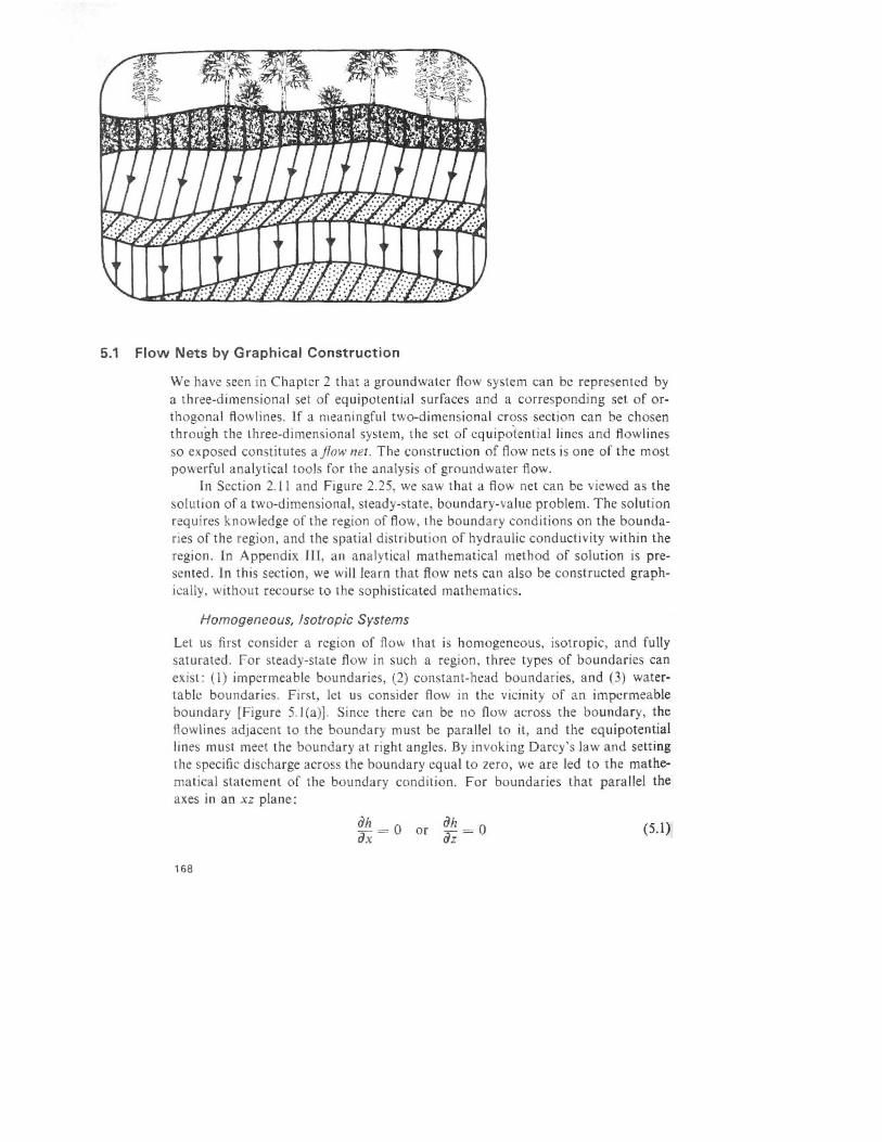
5.1 Flow Nets by Graphical Construction

We have seen in Chapter 2 that a groundwater flow yste m can be repre ented by a three-dimensional set of equipotential surfaces and a corresponding set of or­thogonal flowline . If a meaningful two-dimensional cross section can be chosen through the three-dimensional ystem, the set f equipotential lmes and flowline so e po ed constitutes a flow net . The! construction of flow nets i one of the most powerful analytical tools for the ana lysi of ground water flow.

Jn Section 2.11 and Figure 2.25, we saw that a flo w net can be viewed as the solution of a two-dimensional, steady- tate, boundary-va lue problem. The solution requires knowledge of the region of flo w. the boundary conditions on the bounda­ries of the region, and the patial distribution of hydraulic conducti ily within the region. ln Appendix III, an analytical mathematical method of solution is pre­sented. In this section, we wi ll learn that flow nets can also be constructed graph­ically. without recourse to the ophisticated mathemat ic .

Homogeneous, Isotropic Systems

Let u first consider a region of flow t.hat is homogeneous, isotropic, and fully aturated . For steady-state flow in such a region. three types of boundaries can

e 1st : ( 1) impermeable boundarie , (2) constant-head boundaries. and (3) water­table boundarie . Fir t, let us con ider flow in the v1ci nity of , n impermeable boundary [Figure 5.l(a)]. Since there can be no flow across the boundary, the flowlines adjacent to the boundary must be parallel to it, and the equipotential lines must meet the bound ry at nght angles. By invoking Darcy's Jaw and setting the specific discharge across the boundary equal to zero, we are led to the mathe­matical statement of the boundary condition. For boundaries that parallel the axes in an xz plane:

ah _ 0 or az­ (5.1)

168

/

( 0 ) (b) l c)

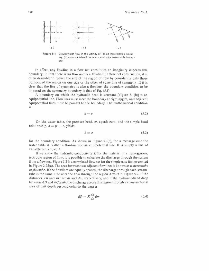
Figure 5.1 Groundwater flow in the vicin tty of (a) an tmpermeable bound. ary, (b) a consta nt-head boundary, and (c) a water-table bound­ary.

169 Flow Nets I Ch. 5

In effect, any flowline in a flow net constitutes an imaginary impermeable boundary, in that there is no flow across a flowline . In flow-net construction, it is often desirable to reduce the size of the region of flow by considermg only those portions of the region on one side or the other of some line of symmetry . If it is clear that the line of symmetry is also a flowline , the boundary condition to be imposed on the symmetry boundary is that of Eq. (5 .1 ).

A boundary on which the hydraulic head i constant [Figure 5.I(b)] is an equipotential line. Flowlines must meet the boundary at right angles, and adjacent equipotential lines must be parallel to the boundary. The mathematical condition is

h=c (5 .2)

On the water table, the pressure head, 'If, equals zero, and the simple head relationship, h = 'II + z, yields

h=z (5.3)

for the boundary condition . As shown in Figure 5. 1 (c), for a recharge case the wa ter table is neither a flowline nor an equipotential line. It is simply a line of variable but known h.

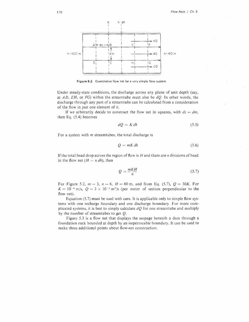
If we know the hydraulic conductivity K for the material in a homogenous, i otropic region of flow, it is possible to calculate the discharge through the system from a flow net. Figure 5.2 is a completed flow net for the simple case first presented in Figure 2.25(a). The area between two adjacent flowlines i known as a streamtube or jfowtube. If the flowlines are equally spaced, the discharge through each stream­tube is the same. Consider the flow through the region A BCD in Figure 5.2. If the distances A B and BC are ds and dm, respectively, and if the hydraulic-head drop between AD and BC is dh, the discharge across this region through a cross-sectional area of unit depth perpendicular to the page is

dhdQ = K-dm ds

(5.4)

h -dh I

h =100 m

__,_1__--;--1~ d 0 E I IF

--'-----.~ d 0

H j IG

--;-,­ ---'­: >~ d 0

Fig ure 5.2 Quantitative flow net for a very simple flow system.

Flow Nets I Ch 5170

Under steady-state conditions, the discharge across any plane of tmit depth ( ay, at AD. EH, or FG) within the streamtube must al o be dQ. In other words, the discharge through any part of a streamtu be can be calculated from a conside.ration of the flow in just one element of it.

If we arbitrarily decide to con truct the flow net in quare , with ds = dm, then Eq. (5.4) becomes

dQ = Kdh (5.5)

For a system with m streamtubes, the total di charge is

Q = mKdh (5.6)

If the total head drop across the region of flow isH and there are n divisions of head in the flow net (H = n dh), then

mKHQ = -n

(5.7)

For Figure 5.2, m = 3, 11 = 6, H = 60 m, and from Eq. (5.7), Q = 30K. For K = JO-• m/s, Q = 3 x JO-l m 3/s (per meter of ection perpendicular to the flow net).

Equation (5.7) mu t be used with care. It is applicable only to simple flow sys­tems with one recharge boundary and one discharge boundary. For more com­plicated systems, it is best to simply calculate dQ for one streamtube and multiply by the number of streamtubes to get Q.

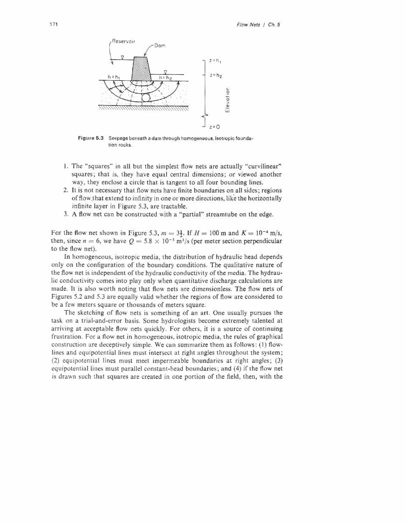
Figure 5.3 is a flow net that displays the eepage beneath a dam through a foundation rock bounded at depth by an impermeable boundary. Jt can be used to make three additional points about flow-net construction .

c: 0

,.0

"' UJ

Figure 6.3 Seepage beneath a dam through homogeneous, isotropic fou nda­tion rocks.

171 Flow Nets I Ch. 5

l. The "squares" in all but the simplest flow nets are actually "curvilinear" squares; that is, they have equal central dimensions; or viewed another way, they enclose a circle that is tangent to all four bounding lines .

2. It is not nece sary that flow nets have finite boundaries on all sides; regions of flow .that extend to infinity in one or more directions, like the horizontally infinite layer in Figure 5.3, are tractable.

3. A flow net can be constructed with a "partia l ' streamtube on the edge.

For the flow net shown in Figure 5.3, m = 3l If H = 100m and K = IQ-• m/s, then, mce n = 6, we have Q = 5.8 x IQ- 3 m 3( (per meter section perpendicular to the flow net).

In homogeneous, isotropic media, the distribution of hydraulic head depends only on the onfiguration of the boundary conditions. The qua)jtative nature of the flow net is independent of the hydraulic conductivity of the media. The hydrau­lic conductivi ty comes into play only when quantitati e discharge calculations are made. It is also worth noting that flow nets are d imensionless. The flow nets of Figures 5.2 and 5.3 are equally valid whether the region of flow are considered to be a few meters square or thousands of meters square.

The sketching of flow nets is something of an art. One usually pursues the ta k on a tri al-and-error basis. Some hydrologists become extremely talented at a rriving at accepta ble flow nets quickly. For others. it i source of cont inuing frustration . For a flow net in homogeneous, i otropic media, the rules of graphical construction a re deceptively si mple. We can summarize them as follows : (I) flow ­lines and equipotential lines must inter ec a t right a ngles throughout the system; (2) equi potentia l lines must meet impermeable boundarie at right angles; (3) equipotential lines must parallel constant-head boundaries~ and (4) if the flow net is drawn uch that square are created in one portion of the field, then, with the

172 Flow Nets I Ch. 5

pos ible exception of partial flow tubes at the edge, squares must exist throughout the entire field.

Heterogeneous Systems and the Tangent Law

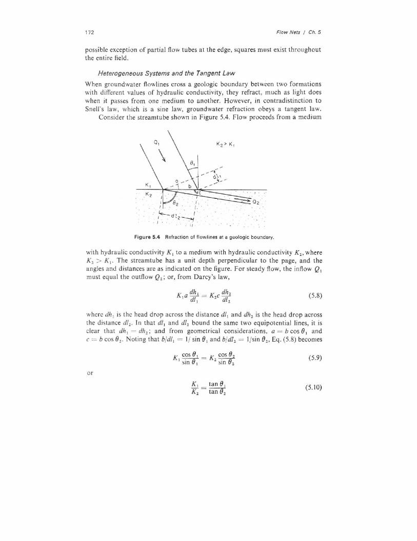
When groundwater flowlines cross a geologic boundary between two formations with different values of hydraulic conductivi ty, they refract, much as light doe when it passes from one medium to another. However, in contradi tinction to Snell's law, which is a sine law, groundwater refraction obeys a tangent law.

Con ider the streamtube shown in Figure 5.4. Flow proceeds from a medium

K, -· . •'

82 . f , I . / . .

. t......_ . I . . ' .I _ d!2~

. . I . . .,, Figure 5.4 Refraction of flowlmes at a geologic bo undary.

with hydraulic conductivity K 1 to a medium with hydraulic conductivity K 2 , where K 2 > K,. The streamtube has a unit depth perpend icular to the page, and the angle and distances are as indicated on the figure. For steady flow, the inflow Q, must equal the outflow Q1 ; or, from Darcy's law,

(5.8)

where dh, i the head drop across the distance dl, and dh 2 is the head drop across the di lance df2 . In that dl, and d/2 bound the same two equipotential lines, it is clear that Jh, = dh2 ; and from geometrical considerations. a = b cos 0, and c = b cos 02 • Not ing that b/dl, = 1/ sin 0, and b/dl 1 = 1/sin 82 Eq. (5.8) becomes

(5.9)

or

(5.10)