focusing 3d measured field-probe data to image a compact
TRANSCRIPT
Focusing 3D Measured Field-Probe Data To Image A
Compact Range Reflector
Scott T. McBride
MI Technologies
1125 Satellite Blvd, Suite 100, Suwanee, GA 30024
Abstract—A diagnostic technique was published over 20 years
ago on imaging compact-range reflectors by focusing plane-polar
field-probe data. At that time, only synthesized data had been
evaluated. Since then, a few reflectors have exhibited
performance lower than expected, and this technique has been
successfully employed to improve that performance based on
their measured data. This paper reviews the technique and
discusses the results of processing those measured data sets.
The technique produces an image of the estimated field
amplitudes at the reflector surface that do not contribute to the
desired quiet-zone plane wave. Point sources, line sources, and
deformations over an area have all been successfully identified,
often outside the projected circular boundary of the field-probe
data. All measurements to date have used very coarse angular
spacing with acceptable degradation in image quality.
I. INTRODUCTION
If field-probe data in a compact range are not within specifications, the options for finding the root cause are often limited. The data collected by the field probe can provide significant information in the search for a solution.
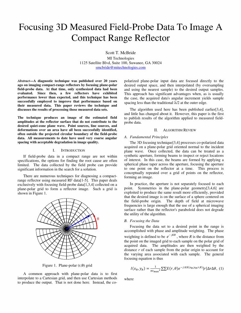
There are numerous techniques for diagnosing a compact-range reflector using measured RF data[1-5]. This paper deals exclusively with focusing field-probe data[1,3,4] collected on a plane-polar grid to form a reflector image. Such a grid is shown in Figure 1.
Figure 1. Plane-polar (r,θ) grid
A common approach with plane-polar data is to first interpolate to a Cartesian grid, and then use Cartesian methods to produce the output. That is not done here. Instead, the co-
polarized plane-polar input data are focused directly to the desired output space, and then interpolated (by oversampling and using the nearest sample) to the desired output samples. This approach has significant advantages when, as is usually the case, the acquired data's angular increment yields sample
spacing less than the traditional λ/2 at the outer edge.
The algorithm used here has been published earlier[3,4], and little has changed about it. However, this paper is the first to publish results of the algorithm applied to measured field-probe data.
II. ALGORITHM REVIEW
A. Fundamental Principles
The 3D focusing technique[3,4] processes co-polarized data acquired on a plane-polar grid oriented normal to the incident plane wave. Once collected, the data can be treated as a synthetic aperture, forming beams to inspect or reject locations of interest. In this case, the beams are formed by applying a spherical phase taper across the aperture, focusing the aperture to one point on the reflector at a time. This process is conceptually repeated over a grid of points on the reflector, forming an image.
In practice, the aperture is not separately focused to each point. Symmetries in the plane-polar geometry[3,4,6] are exploited to produce the same result more efficiently, provided that the desired image is on the surface of a sphere centered on the field-probe origin. The depth of field at microwave frequencies is large enough that the use of a spherical imaging surface rather than the reflector's paraboloid does not degrade the utility of the algorithm.
B. Focusing the Data
Focusing the data set to a desired point in the range is accomplished with phase and amplitude weighting. The phase
weighting is defined to be jKR
e−
, where R is the distance from
the point on the imaged grid to each sample on the polar grid of acquired data. The amplitudes are then weighted by the distance r of each sample from the polar origin to account for the varying area associated with each sample. The general focusing equation is thus
���� , ��� =
�� ��
∑∑���, ����� ����� ,��,�,��|�|Δ�Δ�, (1)
where
I is the image produced
r is the radial coordinate of the measured field
� is the angular coordinate of the measured field
E is the measured field (after main-beam removal)
is the wave number !
"
#��� , �� , �, �� is the distance between each field
location (r, θ) and the reflector coordinate ��� , ���.
Rather than focus the measured data to each point on the reflector independently, symmetries resulting from the plane-polar acquisition geometry and our choice of a spherical image surface are exploited[3,4,6]. As an example, let's imagine that we have a single horizontal scan of field-probe data, and that we want to compute the focused image on a regular grid of xR and yR projected onto a spherical surface centered on the field-probe origin. It is not difficult to determine that the 3D image from this one scan will be a function only of xR, such that a single value of yR can be used and the result replicated (or extruded) to all other values of yR. Similarly, a single vertical cut of field probe data will yield an image that is only a function of yR, such that 1D focusing along yR can be followed by a replication or extrusion along xR. If we acquired just two scans, then the result of (1) would equal the coherent sum of the two complex images from the single scans.
The exactness of this symmetry falls apart when using θ angles whose tangents are not rational[3], since the grid of
output points will not line up when rotated by such a θ angle. Therefore, we must somehow interpolate our extruded 1D output onto the output grid. This is easily and effectively accomplished by oversampling the 1D output and finding the closest point in the extrusion. In the Ka-band example below, the time spent focusing was reduced by more than a factor of 50. The total time spent processing the 28 Ka-band frequencies was less than five minutes. A four-hour turnaround would be much less convenient.
As the distance between the measured data and the imaged spherical surface approaches infinity, the phase taper needed to focus the data becomes linear. At this point, a 1D FFT of each radially weighted scan along the linear axis can be performed rather than a 1D focusing operation, and this becomes the polar-coordinate Fourier transform[6], which was originally derived from this work.
C. Sampling Criteria
As with any spatial-array technique, there are minimum criteria for sampling density that depend upon the spatial bandwidth of the measured signal. The criteria for this algorithm are similar to those for the related polar-coordinate Fourier transform[6], where only the spacing along the linear (radial) axis affects aliasing. The conventional rule of thumb is
that the radial spacing should be λ/2, where λ is the smallest wavelength being sampled. However, larger increments can be used provided that all radiation is coming from a limited angle relative to the field probe's aperture normal.
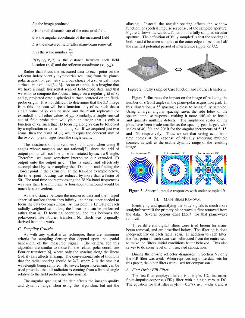
The angular spacing of the data affects the image's quality and dynamic range when using this algorithm, but not the
aliasing. Instead, the angular spacing affects the window function, or spectral impulse response, of the sampled aperture. Figure 2 shows the window function of a fully sampled circular aperture. The definition of 'fully sampled' is that the spacing in
both r and θ between samples at the outer edge is less than half
the smallest potential period of interference ripple, or λ/2.
⇔
Figure 2. Fully sampled Circ function and Fourier transform
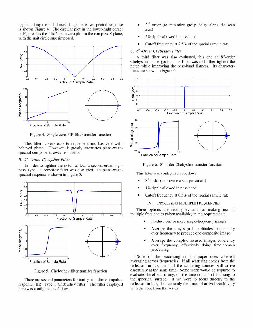
Figure 3 illustrates the impact on the image of reducing the
number of θ (roll) angles in the plane-polar acquisition grid. In
this illustration, a 5° spacing is close to being fully sampled. Using a larger angular spacing raises the side lobes of the spectral impulse response, making it more difficult to locate and quantify multiple defects. The amplitude scales of the plots have been made smaller as the spacing gets larger, with scales of 40, 30, and 20dB for the angular increments of 5, 15,
and 45°, respectively. Thus, we see that saving acquisition time comes at the expense of visually resolving multiple sources, as well as the usable dynamic range of the resulting image.
Figure 3. Spectral impulse responses with under-sampled θ
III. MAIN-BEAM REMOVAL
Identifying and quantifying the stray signals is much more straightforward if the primary plane wave is first removed from the data. Several options exist [2,5,7] for that plane-wave removal.
Three different digital filters were tried herein for main-beam removal, and are described below. The filtering is done independently on each radial scan. In addition to each filter, the first point in each scan was subtracted from the entire scan to make the filters' initial conditions better behaved. This also serves to do some level of untruncated subtraction.
During the on-site reflector diagnoses in Section V, only the FIR filter was used. When reprocessing those data sets for this paper, the other filters were used for comparison.
A. First-Order FIR Filter
The first filter employed herein is a simple, 1D, first-order, finite-impulse-response (FIR) filter with a single zero at DC. The equation for that filter is y[n] = 0.5*(x[n-1] – x[n]), and is
applied along the radial axis. Its plane-wave-spectral response is shown Figure 4. The circular plot in the lower-right corner of Figure 4 is the filter's pole-zero plot in the complex Z plane, with the unit circle superimposed.
Figure 4. Single-zero FIR filter transfer function
This filter is very easy to implement and has very well-behaved phase. However, it greatly attenuates plane-wave-spectral components away from zero.
B. 2nd
-Order Chebyshev Filter
In order to tighten the notch at DC, a second-order high-pass Type 1 Chebyshev filter was also tried. Its plane-wave-spectral response is shown in Figure 5.
Figure 5. Chebyshev filter transfer function
There are several parameters for tuning an infinite-impulse-response (IIR) Type 1 Chebyshev filter. The filter employed here was configured as follows:
• 2nd
order (to minimize group delay along the scan axis)
• 5% ripple allowed in pass band
• Cutoff frequency at 2.5% of the spatial sample rate
C. 8th
-Order Chebyshev Filter
A third filter was also evaluated, this one an 8th-order
Chebyshev. The goal of this filter was to further tighten the notch while improving the pass-band flatness. Its character-istics are shown in Figure 6.
Figure 6. 8th
-order Chebyshev transfer function
This filter was configured as follows:
• 8th order (to provide a sharper cutoff)
• 1% ripple allowed in pass band
• Cutoff frequency at 0.5% of the spatial sample rate
IV. PROCESSING MULTIPLE FREQUENCIES
Three options are readily evident for making use of multiple frequencies (when available) in the acquired data:
• Produce one or more single-frequency images
• Average the stray-signal amplitudes incoherently over frequency to produce one composite image
• Average the complex focused images coherently over frequency, effectively doing time-domain processing
None of the processing in this paper does coherent averaging across frequencies. If all scattering comes from the reflector surface, then all the scattering sources will arrive essentially at the same time. Some work would be required to evaluate the effect, if any, on the time-domain of focusing to the spherical surface. If we were to focus directly to the reflector surface, then certainly the times of arrival would vary with distance from the vertex.

The incoherent averaging employed here emphasizes those scattering sources whose locations are consistent throughout the band. The artifacts introduced by undersampling and measurement noise are attenuated somewhat with the use of multiple frequencies, so the resulting image is clearer.
V. MEASURED DATA SETS
Data have been collected for at least six facilities over the last 20 years and run through this focusing algorithm. Most of those facilities had no reflector issues such that the resulting images are uninteresting. Two reflectors' measured data yielded information that led to on-site remedies that put those facilities in spec. Those two reflectors are discussed in this section.
A. MI-506C
This reflector was installed overseas, and initially did not meet specifications. It had received rough handling in transit, traveling by boxcar rather than the specified air-ride trailer. A laser tracker was sent to re-measure the surface, but was delayed in customs. While waiting for the laser, data were acquired for this focusing algorithm, and a workable solution was found based primarily on the focused results.
The data were acquired at a single frequency of 18 GHz.
The radial spacing was about 3/4 λ, which is sufficient if all stray signal comes from the reflector. The field probe's extent was the same size as the quiet zone, such that no data were acquired outside of the quiet zone. The angular spacing of the
plane-polar grid was 5°, which was nearly 10 times the spacing needed to fully sample the quiet zone's 1.8m diameter at that frequency. The image resulting from focusing the measured data is shown in Figure 7, with the approximate serration outline and field-probe data boundary superimposed.
Figure 7 suggests that the dominant scattering source is located near the two top-center serrations. A very faint triangle extends up onto the right-hand serration in that pair. A similar but lower-amplitude shape is evident near the bottom of the reflector body. The clouds of points in the upper corners are believed to be artifacts (side lobes) of the dominant scatterer
resulting from the very coarse θ increment.
Figure 7. MI-506C focused image (FIR filter)
The processing was repeated using the 2nd
-order Chebyshev filter for main-beam removal. Those results are shown in Figure 8. Perhaps the most significant difference between the two filters is a 14dB increase in the reported stray signal level relative to the primary plane wave. This is likely due to the Chebyshev's lower attenuation of each spherical wave's plane-wave spectrum. The higher stray-signal levels seem more believable given the level of amplitude ripple in the measured data.
Figure 8. MI-506C focused image (2nd
-order Chebyshev)
The 8th
-order Chebyshev was also applied to the data, and that result is shown in Figure 9. Here we see that more anomalies have appeared closer to the reflector center. It seems likely that this is due to the narrower notch, where the filter puts less attenuation on spherical waves coming from that region.
Figure 9. MI-506C focused image (8th
-order Chebyshev)
From the location and shape of the dominant scattering source, it seems likely that it was coming from some combination of
• Reflector body distortion
• Serration seam anomalies
• Serration alignment
Of these three potential error sources, the serration alignment was by far the easiest to address. Since the reflector already had its protective coating of latex paint over the silvered surface, any seam or surface repair would have required removing that latex.
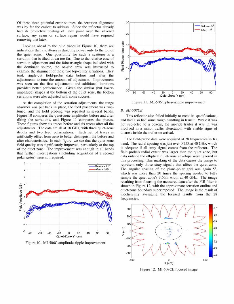
Looking ahead to the blue traces in Figure 10, there are indications that a scatterer is directing power only to the top of the quiet zone. One possibility for such a scatterer is a serration that is tilted down too far. Due to the relative ease of serration adjustment and the faint triangle shape included with the dominant source, the on-site crew was instructed to examine the alignment of those two top-center serrations. They took single-cut field-probe data before and after the adjustments to tune the amount of adjustment. Improvement was seen on the first adjustment, and additional iterations provided better performance. Given the similar (but lower-amplitude) shapes at the bottom of the quiet zone, the bottom serrations were also adjusted with some success.
At the completion of the serration adjustments, the range absorber was put back in place, the feed placement was fine-tuned, and the field probing was repeated in several bands. Figure 10 compares the quiet-zone amplitudes before and after tilting the serrations, and Figure 11 compares the phases. These figures show six traces before and six traces after all the adjustments. The data are all at 18 GHz, with three quiet-zone depths and two feed polarizations. Each set of traces is artificially offset from zero to better distinguish the before and after characteristics. In each figure, we see that the quiet-zone field quality was significantly improved, particularly at the top of the quiet zone. The improvement was enough in all bands that further investigations (including acquisition of a second polar raster) were not required.
Figure 10. MI-506C amplitude-ripple improvement
Figure 11. MI-506C phase-ripple improvement
B. MI-508CE
This reflector also failed initially to meet its specifications, and had also had some rough handling in transit. While it was not subjected to a boxcar, the air-ride trailer it was in was involved in a minor traffic altercation, with visible signs of distress inside the trailer on arrival.
The field-probe data were acquired at 28 frequencies in Ka
band. The radial spacing was just over 0.75λ at 40 GHz, which is adequate if all stray signal comes from the reflector. The field probe's radial extent was larger than the quiet zone, but data outside the elliptical quiet-zone envelope were ignored in this processing. This masking of the data causes the image to represent only those stray signals that affect the quiet zone.
The angular spacing of the plane-polar grid was again 5°, which was more than 20 times the spacing needed to fully sample the quiet zone's 3.66m width at 40 GHz. The image resulting from focusing the measured data after the FIR filter is shown in Figure 12, with the approximate serration outline and quiet-zone boundary superimposed. The image is the result of incoherently averaging the focused results from the 28 frequencies.
Figure 12. MI-508CE focused image
Processing was duplicated using the 2nd
-order Chebyshev filter. The resulting image (not shown) was nearly identical, except the reported stray signal was about 10 dB higher than the levels in Figure 12. The 8
th-order Chebyshev was then
selected in the processing, and its results are shown in Figure 13. Here we again see that new anomalies are reported closer to the center of the reflector. Note, however, that the usable dynamic range (before significant clutter appears) has been lowered to 5 dB.
Figure 13. MI-508CE image with 8th
-order Chebyshev
The image in Figure 12, along with measured laser data, was used to address reflector issues. These remedies were sufficient to bring the reflector within its requirements.
VI. REFELCTED STRAY SIGNALS
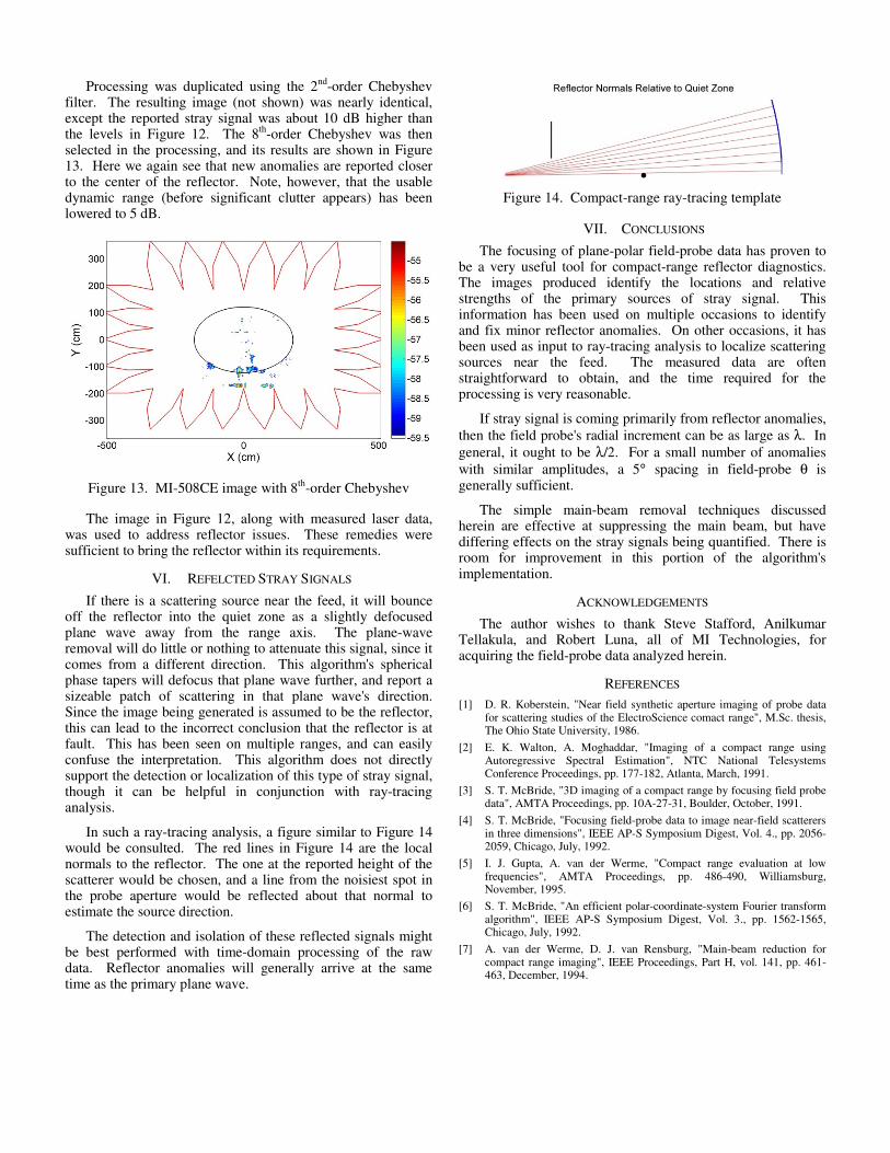
If there is a scattering source near the feed, it will bounce off the reflector into the quiet zone as a slightly defocused plane wave away from the range axis. The plane-wave removal will do little or nothing to attenuate this signal, since it comes from a different direction. This algorithm's spherical phase tapers will defocus that plane wave further, and report a sizeable patch of scattering in that plane wave's direction. Since the image being generated is assumed to be the reflector, this can lead to the incorrect conclusion that the reflector is at fault. This has been seen on multiple ranges, and can easily confuse the interpretation. This algorithm does not directly support the detection or localization of this type of stray signal, though it can be helpful in conjunction with ray-tracing analysis.
In such a ray-tracing analysis, a figure similar to Figure 14 would be consulted. The red lines in Figure 14 are the local normals to the reflector. The one at the reported height of the scatterer would be chosen, and a line from the noisiest spot in the probe aperture would be reflected about that normal to estimate the source direction.
The detection and isolation of these reflected signals might be best performed with time-domain processing of the raw data. Reflector anomalies will generally arrive at the same time as the primary plane wave.
Figure 14. Compact-range ray-tracing template
VII. CONCLUSIONS
The focusing of plane-polar field-probe data has proven to be a very useful tool for compact-range reflector diagnostics. The images produced identify the locations and relative strengths of the primary sources of stray signal. This information has been used on multiple occasions to identify and fix minor reflector anomalies. On other occasions, it has been used as input to ray-tracing analysis to localize scattering sources near the feed. The measured data are often straightforward to obtain, and the time required for the processing is very reasonable.
If stray signal is coming primarily from reflector anomalies,
then the field probe's radial increment can be as large as λ. In
general, it ought to be λ/2. For a small number of anomalies
with similar amplitudes, a 5° spacing in field-probe θ is generally sufficient.
The simple main-beam removal techniques discussed herein are effective at suppressing the main beam, but have differing effects on the stray signals being quantified. There is room for improvement in this portion of the algorithm's implementation.
ACKNOWLEDGEMENTS
The author wishes to thank Steve Stafford, Anilkumar Tellakula, and Robert Luna, all of MI Technologies, for acquiring the field-probe data analyzed herein.
REFERENCES
[1] D. R. Koberstein, "Near field synthetic aperture imaging of probe data for scattering studies of the ElectroScience comact range", M.Sc. thesis, The Ohio State University, 1986.
[2] E. K. Walton, A. Moghaddar, "Imaging of a compact range using Autoregressive Spectral Estimation", NTC National Telesystems Conference Proceedings, pp. 177-182, Atlanta, March, 1991.
[3] S. T. McBride, "3D imaging of a compact range by focusing field probe data", AMTA Proceedings, pp. 10A-27-31, Boulder, October, 1991.
[4] S. T. McBride, "Focusing field-probe data to image near-field scatterers in three dimensions", IEEE AP-S Symposium Digest, Vol. 4., pp. 2056-2059, Chicago, July, 1992.
[5] I. J. Gupta, A. van der Werme, "Compact range evaluation at low frequencies", AMTA Proceedings, pp. 486-490, Williamsburg, November, 1995.
[6] S. T. McBride, "An efficient polar-coordinate-system Fourier transform algorithm", IEEE AP-S Symposium Digest, Vol. 3., pp. 1562-1565, Chicago, July, 1992.
[7] A. van der Werme, D. J. van Rensburg, "Main-beam reduction for compact range imaging", IEEE Proceedings, Part H, vol. 141, pp. 461-463, December, 1994.