lectures 8, 9 and 10 finite difference discretization of hyperbolic equations: linear problems
TRANSCRIPT

Lectures 8, 9 and 10
Finite Difference Discretization of Hyperbolic Equations:
Linear Problems

First Order Wave Equation
INITION BOUNDARY VALUE PROBLEM (IBVP)
Initial Condition:
Boundary Conditions:

First Order Wave Equation
Solution
Characteristics
General solution

First Order Wave Equation
Solution

First Order Wave Equation
Solution

First Order Wave Equation
Stability

Model Problem
Initial condition:
Periodic Boundary conditions:
constant

Model ProblemExample
Periodic Solution (U>0)

Finite DifferenceSolution
Discretization
Discretize (0,1) into J equal intervals
And (0,T) into N equal intervals

Finite DifferenceSolution
Discretization

Finite DifferenceSolution
Discretization
NOTATION:• approximation to
• vector of approximate values at time ;
• vector of exact values at time ;

Finite DifferenceSolution
Approximation
For example … for ( U > 0 )
Forward in Time Backward (Upwind) in Space

Finite DifferenceSolution
First Order Upwind Scheme
suggests …
Courant number C =

Finite DifferenceSolution
First Order Upwind Scheme
Interpretation
Use Linear Interpolation
j – 1, j

Finite DifferenceSolution
First Order Upwind Scheme
Explicit Solution
no matrix inversion
exists and is unique

Finite DifferenceSolution
First Order Upwind Scheme
Matrix Form
We can write

Finite DifferenceSolution
First Order Upwind Scheme
Example

ConvergenceDefinition
The finite difference algorithm converges if
For any initial condition .

ConsistencyDefinition
For all smooth functions
when .
The difference scheme ,
is consistent with the differential equation
if:

ConsistencyFirst Order Upwind Scheme
Difference operator
Differential operator

ConsistencyFirst Order Upwind Scheme
First order accurate in space and time

Truncation Error
Insert exact solution into difference scheme
Consistency

Stability
The difference scheme is stable if:
There exists such that
for all ; and n, such that
Definition
Above condition can be written as

StabilityFirst Order Upwind Scheme
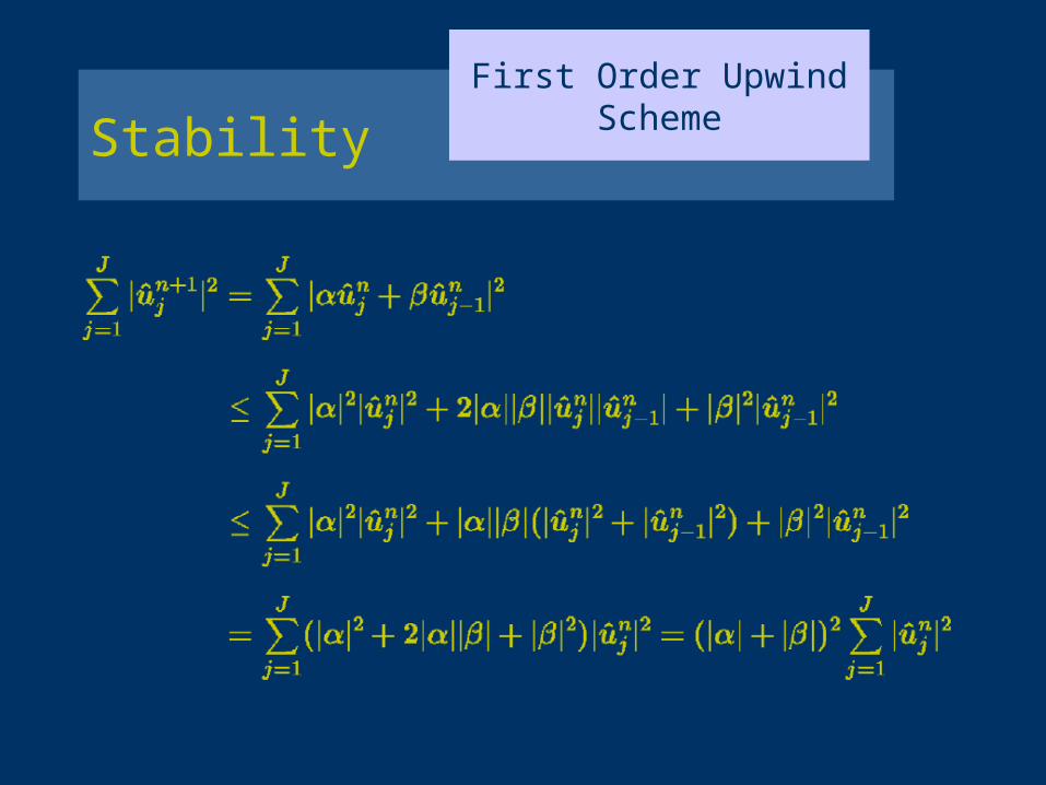
StabilityFirst Order Upwind Scheme

Stability
Stable if
Upwind scheme is stable provided

Lax EquivalenceTheorem
A consistent finite difference scheme for a partial differential equation for which the initial value problem is well-posed is convergent if and only if it is stable.

Lax EquivalenceTheorem
Proof
( first order in , )

Lax EquivalenceTheorem
First Order Upwind Scheme
• Consistency:• Stability: for• Convergence
or
and are constants independent of ,

Lax EquivalenceTheorem
First Order Upwind Scheme
Example
Solutions for:
(left)
(right)
Convergence is slow !!

CFL ConditionDomains of dependence
Mathematical Domain of Dependence of
Set of points in where the initial or boundary
data may have some effect on .
Numerical Domain of Dependence of
Set of points in where the initial or boundary
data may have some effect on .

CFL ConditionDomains of dependence
First Order Upwind Scheme
Analytical Numerical ( U > 0 )

CFL ConditionCFL Theorem
CFL Condition
For each the mathematical domain of de-
pendence is contained in the numerical domain of dependence.
CFL Theorem
The CFL condition is a necessary condition for the convergence of a numerical approximation of a partial differential equation, linear or nonlinear.

CFL ConditionCFL Theorem
Stable Unstable

Fourier Analysis
• Provides a systematic method for determining stability → von Neumann Stability Analysis
• Provides insight into discretization errors

Fourier AnalysisContinuous Problem
Fourier Modes and Properties…
Fourier mode: ( integer )
• Periodic ( period = 1 )
• Orthogonality
•Eigenfunction of

Fourier AnalysisContinuous Problem
…Fourier Modes and Properties
• Form a basis for periodic functions in
• Parseval’s theorem

Fourier AnalysisContinuous Problem
Wave Equation

Fourier AnalysisDiscrete Problem
Fourier Modes and Properties…
Fourier mode: ,
k ( integer )

Fourier AnalysisDiscrete Problem
…Fourier Modes and Properties…
Real part of first 4 Fourier modes

Fourier AnalysisDiscrete Problem
…Fourier Modes and Properties…
• Periodic (period = J)
• Orthogonality

Fourier AnalysisDiscrete Problem
…Fourier Modes and Properties…
• Eigenfunctions of difference operators e.g.,

Fourier AnalysisDiscrete Problem
Fourier Modes and Properties…
• Basis for periodic (discrete) functions
• Parseval’s theorem

Fourier Analysisvon Neumann Stability Criterion
Write
Stability
Stability for all data

Fourier Analysisvon Neumann Stability Criterion
First Order Upwind Scheme…

Fourier Analysisvon Neumann Stability Criterion
…First Order Upwind Scheme…
amplification factor
Stability if which implies

Fourier Analysisvon Neumann Stability Criterion
…First Order Upwind Scheme
Stability if:

Fourier Analysisvon Neumann Stability Criterion
FTCS Scheme…
Fourier Decomposition:

Fourier Analysisvon Neumann Stability Criterion
amplification factor
Unconditionally Unstable Not Convergent
…FTCS Scheme

Lax-WendroffScheme
Time Discretization
Write a Taylor series expansion in time about
But …

Lax-WendroffScheme
Spatial Approximation
Approximate spatial derivatives

Lax-WendroffScheme
Equation
no matrix inversion
exists and is unique

Lax-WendroffScheme
Interpretation
Use Quadratic
Interpolation

Lax-WendroffScheme
Analysis
Consistency
Second order accurate in space and time

Lax-WendroffScheme
Analysis
Truncation Error
Consistency
Insert exact solution into difference scheme

Lax-WendroffScheme
Analysis
Stability
Stability if:

Lax-WendroffScheme
Analysis
Convergence
• Consistency:
• Stability:
• Convergence
and are constants independent of

Lax-WendroffScheme
Domains of Dependence
Analytical Numerical

Lax-WendroffScheme
CFL Condition
Stable Unstable
Lax-WendroffScheme
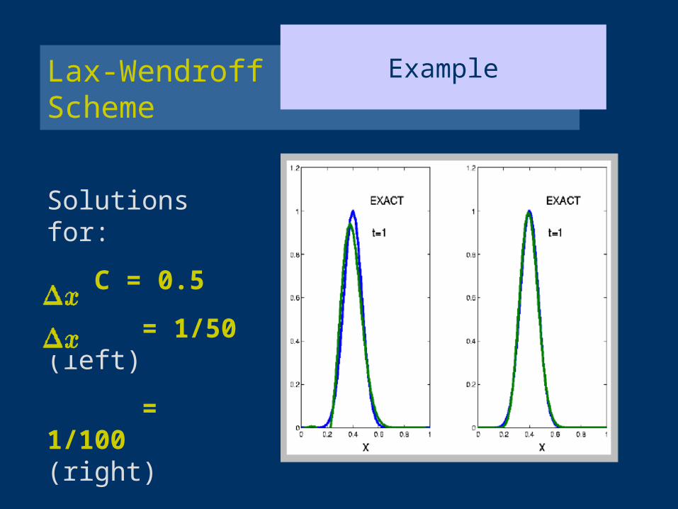
Example
Solutions for:
C = 0.5
= 1/50 (left)
= 1/100 (right)

Lax-WendroffScheme
Example
= 1/100
C = 0.5
Upwind (left)
vs.
Lax-Wendroff (right)

Beam-WarmingScheme
Derivation
Use Quadratic
Interpolation

Beam-WarmingScheme
Consistency and Stability
• Consistency,
• Stability

Method of Lines
Generally applicable to time evolution PDE’s• Spatial discretization
Semi-discrete scheme (system of coupled ODE’s
• Time discretization (using ODE techniques)
Discrete Scheme
By studying semi-discrete scheme we can better
understand spatial and temporal discretization errors

Method of Lines
Notation
approximation to
vector of semi-discrete approximations;

Method of LinesSpatial Discretization
Central difference … (for example)
or, in vector form,

Method of LinesSpatial Discretization
Write semi-discrete approximation as
inserting into semi-discrete equation
Fourier Analysis …

Method of LinesSpatial Discretization
For each θ, we have a scalar ODE
… Fourier Analysis …
Neutrally stable

Method of LinesSpatial Discretization
Exact solution
Semi-discrete solution
… Fourier Analysis …

Method of LinesSpatial Discretization
Fourier Analysis …

Method of LinesTime Discretization
Predictor/Corrector Algorithm …
Model ODE
Predictor
Corrector
Combining the two steps you have

Method of LinesTime Discretization
…Predictor/Corrector Algorithm
Semi-discrete equation
Predictor
Corrector
Combining the two steps you have

Method of LinesFourier Stability Analysis
Fourier Transform

Method of LinesFourier Stability Analysis
Application factor
with
Stability

Method of LinesFourier Stability Analysis
PDE
Semi-discrete
Semi-discrete Fourier
Discrete
Discrete Fourier

Method of LinesFourier Stability Analysis
Path B …
Semi-discrete
Fourier semi-discrete
Predictor
Corrector
Discrete

Method of LinesFourier Stability Analysis
…Path B
• Give the same discrete Fourier equation
• Simpler
• “Decouples” spatial and temporal discretization For each θ, the discrete Fourier equation is the result of discretizing the scalar semi-discrete ODE for the θ Fourier mode

Method of LinesMethods for ODE’s
Model equation: complex- valued
Discretization
EF
EB
CN

Method of LinesMethods for ODE’s
Given and complex-valued
Absolute Stability Diagrams …
(EF) or (EB) or … ;
is defined such that

Method of LinesMethods for ODE’s
…Absolute Stability Diagrams …
EF
EB
CN
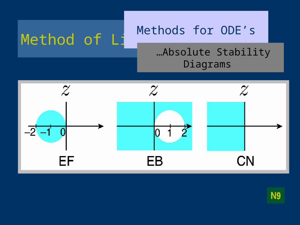
Method of LinesMethods for ODE’s
…Absolute Stability Diagrams

Method of LinesMethods for ODE’s
Application to the wave equation…
For each
Thus,
• (and ) is purely imaginary • for

Method of LinesMethods for ODE’s
…Application to the wave equation…
EF is unconditionally unstable
EB is unconditionally stable
CN is unconditionally stable
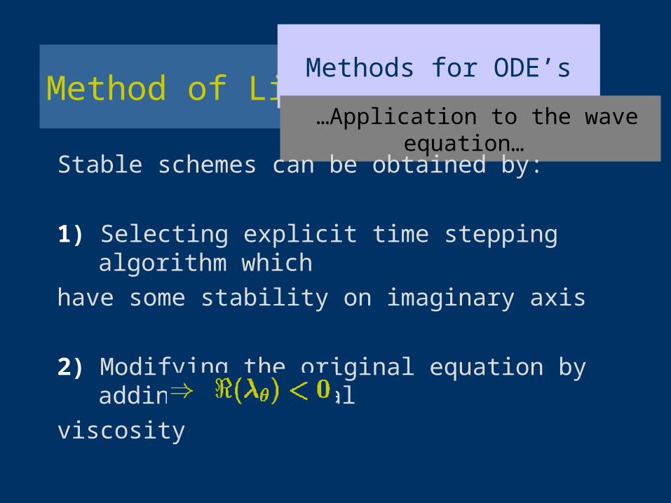
Method of LinesMethods for ODE’s
…Application to the wave equation…
Stable schemes can be obtained by:
1) Selecting explicit time stepping algorithm which
have some stability on imaginary axis
2) Modifying the original equation by adding “artificial
viscosity”

Method of LinesMethods for ODE’s
…Application to the wave equation…
Explicit Time Stepping Scheme
Predictor/Corrector

Method of LinesMethods for ODE’s
…Application to the wave equation…
Explicit Time Stepping Scheme
4 Stage Runge-Kutta

Method of LinesMethods for ODE’s
…Application to the wave equation…
Adding Artificial Viscosity
Additional Term
EF Time First Order Upwind
EF Time Lax-Wendroff

Method of LinesMethods for ODE’s
…Application to the wave equation…
Adding Artificial Viscosity
For each Fourier mode θ,
Additional Term

Method of LinesMethods for ODE’s
…Application to the wave equation…
First Order Upwind Scheme

Method of LinesMethods for ODE’s
…Application to the wave equation
Lax-Wendroff Scheme

Dissipation andDispersion
Model Problem
with and periodic boundary conditions.
Solution

Dissipation andDispersion
Model Problem
represents Decay
dissipation relation
represents Propagation
dispersion relation
For exact solution of
no dissipation
(constant) no dispersion

Dissipation andDispersion
Modified Equation
First Order Upwind
Lax-Wendroff
Beam-Warming

Dissipation andDispersion
Modified Equation
• For the upwind scheme dissipation dominates over dispersion Smooth solutions
• For Lax-Wendroff and Beam-Warming dispersion is the leading error effect Oscillatory solutions ( if not well resolved)
• Lax-Wendroff has a negative phase error• Beaming-Warming has (for ) a positive phase
error

Dissipation andDispersion
Examples
First Order Upwind

Dissipation andDispersion
Examples
Lax-Wendroff (left)
vs.
Beam-Warming (right)

Dissipation andDispersion
Exact Discrete Relations
For the exact solution
, and
For the discrete solution
, and