Hidden Truncation Hyperbolic Distributions, FiniteMixtures Thereof, and Their Application for Clustering

Paula M. Murray∗, Ryan P. Browne∗∗ and Paul D. McNicholas∗

∗Department of Mathematics and Statistics, McMaster University, Ontario, Canada.∗∗Department of Statistics and Actuarial Sciences, University of Waterloo, Ontario, Canada.

Abstract

A hidden truncation hyperbolic (HTH) distribution is introduced and finite mix-tures thereof are applied for clustering. A stochastic representation of the HTH dis-tribution is given and a density is derived. A hierarchical representation is described,which aids in parameter estimation. Finite mixtures of HTH distributions are pre-sented and their identifiability is proved. The convexity of the HTH distribution isdiscussed, which is important in clustering applications, and some theoretical resultsin this direction are presented. The relationship between the HTH distribution andother skewed distributions in the literature is discussed. Illustrations are provided —both of the HTH distribution and application of finite mixtures thereof for clustering.

Keywords: clustering; hidden truncation; hyperbolic distribution; mixture models.

1 Introduction

Broadly, cluster analysis is the process of identifying groups of similar observations withina data set. Model-based clustering is a method for performing cluster analysis that involvesthe fitting of a finite mixture model. Recently, attention has focused on mixtures of flexibleasymmetric distributions and, to this end, we develop a hidden truncation hyperbolic (HTH)distribution and use a mixture thereof to perform flexible model-based clustering. Thismixture model is more general than other mixture models based on truncated distributionsthat have appeared in the literature. A finite mixture model has density

f(x | ϑ) =G∑g=1

πgfg(x | θg), (1)

such that ϑ = (π1, ..., πG,θ1, ...,θG), πg > 0, and∑G

g=1 πg = 1, where x is a p-dimensionaldata vector, πg is the gth mixing proportion, and fg(x | θg) is the gth component density.

1

arX

iv:1

707.

0224

7v2

[st

at.M

E]

20

Jul 2

017

Mixture models have been employed for decades in cluster analysis (e.g., Day, 1969; Wolfe,1963, 1965) and, in fact, McNicholas (2016a) traces the association of mixture models withclustering back to Tiedeman (1955). The Gaussian mixture model has been the most popularapproach and work in this direction has focused on approaches that reduce the number offree parameters in the component covariance matrices (e.g., Banfield and Raftery, 1993;Celeux and Govaert, 1995; McNicholas and Murphy, 2008). Over the past fifteen years orso, these Gaussian mixture modelling approaches have been extended in various ways toaccommodate increasingly complicated applications. Many of these extensions involve usingnon-Gaussian distributions to accommodate component skewness and/or concentration (e.g.,Franczak et al., 2014; Lee and McLachlan, 2014; Lin et al., 2007; McNicholas et al., 2017;Montanari and Viroli, 2010; Murray et al., 2014). Interestingly, beyond certain formulationsof the skew-normal and skew-t distributions (e.g., Lee and McLachlan, 2014; Lin, 2009,2010), models based on truncated distributions have remained relatively unexplored in theclustering literature. A recent review of model-based clustering is given by McNicholas(2016b).

The mixture of HTH distributions developed herein is based on a truncated hyperbolicrandom variable and contains both mixtures of certain formulations of mixtures of skew-t and mixtures of skew-normal distributions as special cases. Some background on hiddentruncation is provided in Section 2 and the HTH distribution is developed in Section 3, alongwith a derivation of the moments of the truncated symmetric hyperbolic distribution. Then,identifiability of finite mixtures of HTH distributions is proved (Section 4.2) and convexity isdiscussed (Section 5). An expectation-conditional maximization (ECM) algorithm is used forfitting mixtures of HTH distributions (Section 6), and clustering performance is illustratedon both real and simulated data (Section 7).

2 Background

2.1 Generalized Inverse Gaussian Distribution

To formulate the HTH distribution, introduce a latent variable W following the generalizedinverse Gaussian (GIG) distribution. The random variable W has density

fGIG(w | ψ, χ, λ) =(ψ/χ)λ/2wλ−1

2Kλ(√ψχ)

exp

(− ψw + χ/w

2

),

for w > 0 with (ψ, χ) ∈ R2+ and λ ∈ R. We write W ∼ GIG(ψ, χ, λ) to indicate that a

random variable W follows a GIG distribution.

2

2.2 Generalized Hyperbolic Distribution

The generalized hyperbolic distribution (GHD; McNeil et al., 2005) has density

fGHD(x | θ) =

χ+ (x− µ)>Σ−1(x− µ)

ψ +α>Σ−1α

(λ−p/2)/2

×(ψ/χ)λ/2Kλ−p/2

(√(ψ +αΣ−1α)

χ+ (x− µ)>Σ−1(x− µ)

)(2π)p/2 | Σ |1/2 Kλ(

√χψ) exp

−(x− µ)>Σ−1α

,

(2)

where x is a p-dimensional data vector, Kλ(·) is the modified Bessel function of the thirdkind with index λ, and θ = (µ,Σ,α, λ, χ, ψ) is a vector of parameters. This density functioncontains a p-dimensional skewness parameter α. The GHD is mean-variance mixture andhas a variety of limiting and special cases (see McNeil et al., 2005). Setting λ = 1 givesa multivariate generalized hyperbolic distribution such that its univariate margins are one-dimensional hyperbolic distributions. Fixing λ = (p+ 1)/2 gives a p-dimensional hyperbolicdistribution, and λ = −1/2 gives the inverse-Gaussian distribution. For λ > 0 and χ → 0,we have a limiting case known as the variance-gamma distribution (Barndorff-Nielsen, 1978).If λ = 1, ψ = 2 and χ → 0, we get the asymmetric Laplace distribution (see Kotz et al.,2001) and if α = 0, we have the symmetric hyperbolic distribution (Barndorff-Nielsen, 1978).Other special and limiting cases include the multivariate normal-inverse Gaussian (MNIG)(Karlis and Meligkotsidou, 2007), a skew-t (Demarta and McNeil, 2005), the multivariate-tand the Gaussian distribution.

Barndorff-Nielsen (1978) introduced generalized hyperbolic distributions to model thegrain sizes of sand and diamonds. Eberlein and Keller (1995) used the hyperbolic distributionto model returns of German equities. (Browne and McNicholas, 2015; Tortora et al., 2015;Morris and McNicholas, 2016) applied the GHD to the context of model-based clustering.

The GHD given in (2) is not identifiable because for any η > 0 we have that the pa-rameters θ = (µ,Σ,α, λ, χ, ψ) and θ∗ = (µ, ηΣ, ηα, λ, χ/η, ηψ) yield the same density. Toensure identifiability, we follow Browne and McNicholas (2015) and set χ = ω and ψ = ωsuch that W ∼ GIG(ω, ω, λ). Using this parameterization and setting the skewness to zero(i.e., α = 0) we obtain an identifiable symmetric hyperbolic distribution with density

h(x | µ,Σ, λ, ω, ω) =

ω + δ(x,µ|Σ)

ω

(λ−p/2)/2Kλ−p/2(√

ωω + δ(x,µ|Σ))

(2π)p/2 | Σ |1/2 Kλ(ω). (3)

where δ(x|µ,Σ) = (x−µ)>Σ−1(x−µ). The symmetric hyperbolic distribution has stochasticrepresentation

X = µ+√WΣ1/2K,

where W ∼ GIG(ω, ω, λ) and K ∼ Np(0, Ip).

3

2.3 The Skew-Normal Distribution

In the past several years, much work has been done on mixture modeling using asymmetricdistributions. One form of the skew-normal distribution that has appeared often in thisliterature is the well-known skew-normal distribution of Sahu et al. (2003) which has thecharacterization

X = µ+ Λ|Z0|+ Z1, (4)

where |Z| = (|Z1|, . . . , |Zp|) for Z ∈ Rp, X is a p-variate skew-normal random variable, Λ isa diagonal matrix that plays the role of a skewness parameter, and[

Z0

Z1

]∼ N2p

([0p0p

],

[Ip 0p0p Σ−ΛΛ>

]).

Note that |Z0| is a half-normal random variable, i.e., |Z0| = U ∼ HN (Iq). Lee and McLach-lan (2013b) refer to this as an “unrestricted” skew-normal distribution because Z0 in thestochastic representation (4) is a random vector rather than a scalar. This is in contrast towhat they call a “restricted” skew-normal distribution, like that of Pyne et al. (2009), whichhas the characterization

X = µ+ λ|Z0|+ Z1, (5)

where [Z0

Z1

]∼ N1+p

([00p

],

[1 0>p0p Σ− λλ>

]).

Note that in the stochastic representation in (5), the random variable Z0 is a scalar and theskewing parameter λ is a vector.

Azzalini et al. (2016) discuss why it is preferable to avoid using the terms “restricted”and “unrestricted” in this way. As such, we will refer to the skew-normal distribution ofSahu et al. (2003) as the SDB distribution herein, referring to the authors’ initials, and wewill refer to the skew-normal distribution of Pyne et al. (2009) as the classical skew-normaldistribution. Models based on the classical formulation are less computationally challengingto fit than their SDB counterparts. However, Lee and McLachlan (2014) argue the SDBdistribution is better at modelling asymmetric data. The HTH distribution contains specialcases that we will call HTHu (q = 1) and HTHm (1 < q ≤ p) which contain the classical andSDB distributions, respectively, as special cases. Here “u” in HTHu refers to the univariateintegral in the HTH density (7) while the “m” in HTHm refers to a multivariate integral(see Section 3).

Herein a hyperbolic random variable is obtained via a relationship with a skew-normalrandom variable Y. A slightly more general formulation of the SDB skew-normal distribu-tion is the canonical fundamental skew-normal (CFUSN) distribution (Arellano-Valle andGenton, 2005) which has density

fSN(y | µ,Σ,Λ) = 2qφp(y | µ,Ω)Φq

Λ>Ω−1(y − µ) |∆

, (6)

4

with location vector µ, scale matrix Σ, and p× q skewness matrix Λ such that ‖Λ>z‖ < 1for any unitary vector z ∈ Rp, where Ω = Σ + ΛΛ>, ∆ = Iq − Λ>Ω−1Λ and φp(· | µ,Σ)and Φq(· | Σ) := Φq(· | µ = 0q,Σ) are the density and cumulative distribution function ofthe multivariate normal distribution, respectively. The CFUSN density (6) is an special caseof the “closed skew-normal” (also called SUN) distribution, and Arellano-Valle and Azzalini(2006) gives an overview and give some the properties of the SUN distribution.

Note that the SDB skew-normal distribution uses a less general form of this density withq = p (Sahu et al., 2003). Arellano-Valle et al. (2007) show we can obtain a p-dimensionalskew-normal random variable Y by

Y = µ+ ΛU + Σ1/2K,

where U ∼ HN(Iq), K ∼ Np(0, Ip), and Σ1/2 denotes the square root of the matrix Σ.Note that HN(Iq) denotes the half-normal distribution with scale matrix Iq. We write Y ∼SNp(µ,Σ,Λ) to denote Y is a skew-normal random variable with density (6). This variantof the skew-normal distribution will be used herein to obtain a HTH random variable X.Arslan (2015) introduce a mean-variance mixture using a GIG distribution and a skew-normal distribution. The resulting model includes a GHD and a skew-normal distributionas special cases.

3 The Hidden Truncation Hyperbolic Distribution

3.1 Overview

Hidden truncation models describe observed variables that are truncated with respect tosome hidden variables; see Arnold and Beaver (2000); Arnold et al. (2002, 1993). Thehidden truncation hyperbolic distribution is developed using a hidden truncated randomvariable and is a “super distribution” as discussed in Section 3.6. We begin by consideringthe symmetric hyperbolic distribution, which is a special case of (2) with zero skewness, i.e.,α = 0. The hidden truncation hyperbolic (HTH) distribution introduced herein regulatesskewness by means of a p × q skewness matrix Λ, where 1 ≤ q ≤ p. Therefore, we can fitspecial cases of our distribution by changing the value of q.

3.2 Stochastic Representation

We generate a p-dimensional random variable X following the HTH distribution through thestochastic representation X = µ+

√WY, where Y ∼ SNp(0,Σ,Λ) and W ∼ GIG(ω, ω, λ).

The HTH density is

fHTH(x|θ) =

2qhp(x|µ,Ω, λ, ω, ω)Hq

[Λ>Ω−1(x− µ)

ω

ω + δ(x|µ,Ω)

1/4 ∣∣∣∣0,∆, λ− (p/2), γ, γ

],

(7)

5

where θ = (µ,Σ,Λ, λ, ω), γ = ω√

1 + δ(x,µ|Ω)/ω, hp(·|µ,Σ, λ, ω, ω) is the density of a p-dimensional symmetric hyperbolic random variable and Hq(·|µ,Σ, λ, ω, ω) is the correspond-ing q-dimensional cdf. Notice that skewness is introduced into this distribution through thep× q skewness matrix Λ. The distribution is also parameterized by a p-dimensional locationparameter µ, p× p scale matrix Σ, ω ∈ R+, and λ ∈ R. To derive this density, we make useof Proposition 1.

Proposition 1. Given W ∼ GIG(ψ, χ, λ), and c ∈ Rq,

E

Φq

(c√W

∣∣∣∣∆) = Hq

c

(ψ

χ

)1/4∣∣∣∣0,∆, λ,√χψ,

√χψ

. (8)

See Supplementary Material S.3 for a proof.Then, to derive the HTH density, we write out the joint density of X and W and then in-

tegrate out W . The conditional density is X|w ∼ SNp(µ, wΣ,√wΛ) and W ∼ GIG(ω, ω, λ)

which gives

fHTH(x|θ) =

∫ ∞0

fSN(y | µ, wΣ,√wΛ)fGIG(w|ω, ω, λ)dw

=

∫ ∞0

2qφp(y | µ, wΩ) Φq

1√w

Λ>Ω−1(y − µ)∣∣∣∆ fGIG(w|ω, ω, λ)dw

= 2qhp(x|µ,Ω, λ, ω, ω)

∫ ∞0

Φq

1√w

Λ>Ω−1(y − µ)∣∣∣∆ fGIG (w|ω + δ(x,µ|Ω), ω, λ) dw

= 2qhp(x|µ,Ω, λ, ω, ω)E

[Φq

1√W

Λ>Ω−1(y − µ)∣∣∣∆] .

Then, applying Proposition 1, we obtain the HTH density given in (7).

3.3 Hierarchical Representation

A random variable X ∼ HTHp(µ,Σ,Λ, λ, ω, ω) can be represented hierarchically by

X | u, w ∼ Np (µ+ ΛU, wΣ) , U | w ∼ HNq (wIq) , W ∼ GIG(ω, ω, λ).

Herein, write r = Λ>Ω−1(x− µ) and δ(x | µ,Ω) = (x− µ)>Ω−1 (x− µ). There follows alisting of the joint and conditional densities pertaining to the variables X, U, and W :

fX,U,W (x,u, w) =wλ−(p+q)/2−1

π(p+q)/22(p−q)/2+1Kλ(ω)|Σ|1/2

× exp

[− 1

2w

ωw2 + ω + (u− r)>∆−1(u− r) + δ(x|µ,Ω)

],

fX,U(x,u) =|Σ|−1/2

π(p+q)/22(p−q)/2Kλ(ω)

ω + (u− r)>∆−1(u− r) + δ(x|µ,Ω)

ω

λ−(p+q)/2/2

×Kλ−(p+q)/2

(√ωω + (u− r)>∆−1(u− r) + δ(x|µ,Ω)

),

6

fX,W (x, w) =wλ−p/2−1|∆|1/2

(π)p/22p/2−q+1Kλ(ω)|Σ|1/2

× exp

[− 1

2w

ωw2 + ω + δ(x|µ,Ω)

]Φq(1/

√w)r|∆,

fU|x,w(u | x, w) =w−q/2

(2π)q/2|∆|1/2Φq(1/√w)r|∆

exp

[− 1

2w

(u− r)>∆−1(u− r)

],

fW |x(w | x) =wλ−(p/2)−1

2Kλ−(p/2)

√ω(ω + δ(x|µ,Ω))

ω

ω + δ(x|µ,Ω)

λ−(p/2)/2

× exp

[−1

2w

ωw2 + ω + δ(x|µ,Ω)

]Φ(r/

√w |∆)

÷Hq

[r

ω

ω + δ(x|µ,Ω)

1/4 ∣∣∣∣0,∆, λ− (p/2),√ωω + δ(x|µ,Ω)

],

and W | x,u ∼ GIGω, ω + (u− r)>∆−1(u− r) + δ(x|µ,Ω), λ− (p+ q)/2. Note that theconditional density of U given X = x is

fU|x(u|x) =1

cλhq(u|r,∆, λ− p/2, γ, γ), (9)

where the support of U is Rq+ and

cλ = Hq

[r

ω

ω + δ(x|µ,Ω)

1/4 ∣∣∣∣0,∆, λ− (p/2), γ, γ

].

It follows that U | w,x ∼ TN(r, w∆;Rq+), where TN(·) denotes the truncated normal dis-

tribution. Also, U | x ∼ THq(r,∆, λ− p/2, γ, γ);Rq+). Here, THq(µ,Σ, λ, ψ, χ;Rq

+) denotesthe q-dimensional symmetric truncated hyperbolic distribution with density

fTH(u | µ,Σ, λ, ψ, χ;Rq+) =

hq(u | µ,Σ, λ, ψ, χ)∫∞0. . .∫∞

0hq(u | µ,Σ, λ, ψ, χ)du

IRq+

(u),

where IRq+

(u) = 1 if u ∈ Rq+ and IRq

+(u) = 0 otherwise. In this way, the symmetric hyperbolic

distribution is truncated to exist only within Rq+.

3.4 Free Parameters and Identifiability

A permutation matrix is a square matrix with exactly one entry of 1 in each row andeach column and 0s elsewhere. Now, if P is a permutation matrix, then P>U has thesame distribution as U ∼ HN (Iq). Therefore, Λ in our HTH distribution is unique up topermutations applied to the right, i.e., fHTH(x | θ) = fHTH(x | θ∗) for all x ∈ Rp, whereθ = (µ,Σ,Λ, λ, ω) and θ∗ = (µ,Σ,Λ∗, λ, ω), if there exists a permutation matrix P such

7

that Λ∗ = ΛP. Because Λ is unique up to permutations applied to the right, it has pq freeparameters — the permutation matrix simply changes the position of the elements and notthe actual values of the elements. Accordingly, sorting the Λ by the norm of the columnsor some other sorting method is needed to ensure that our factor-like model is identifiable,i.e., to take away the caveat about permutations applied to the right.

3.5 Moments

3.5.1 Notation

In this section, we derive the first two moments of the truncated symmetric hyperbolic dis-tribution. These moments have not previously appeared in the literature. Here we introducethe notation used in this section. Consider an n-vector b and an n× n matrix C. Use br todenote the rth element of b, and let b−r denote the (n−1)-vector that results from removingthe rth element from b. Let brs denote the 2-vector (br, bs)

>, and use b−rs to denote the(n − 2)-vector that results from removing the rth and sth elements from b. Let crs denotethe element in the rth row and sth column of C, and use C−rs to denote the (n−2)×(n−2)matrix that results from removing the rth row and sth column from C. Use Crs to denotethe 2× 2 matrix (

crr crscsr css

),

and let [C]rs denote the element in the rth row and sth column of C.

3.5.2 Univariate Case

Where Y is a univariate random variable following the truncated symmetric hyperbolicdistribution, i.e., Y ∼ TH1(µ, σ2, λ, ω, ω), and truncated to exist on the domain [l1, l2], thefirst and second moments of Y are given by

E(Y ) = µ+ σ2Rλ(ω)

h1(l1 | θ[λ+1])− h1(l2 | θ[λ+1])

H1(l2 | θ[λ])−H1(l1 | θ[λ])

and

E(Y 2) = σ2Rλ(ω)

H1(l2 | θ[λ+1])−H1(l1 | θ[λ+1])

H1(l2 | θ[λ])−H1(l1 | θ[λ])+l1h1(l1 | θ[λ+1])− l2h1(l2 | θ[λ+1])

H1(l2 | θ[λ])−H1(l1 | θ[λ])

−h1(l2 | θ[λ+1])− h1(l1 | θ[λ+1])

H1(l2 | θ[λ])−H1(l1 | θ[λ])

,

respectively, where θ[λ] = (µ, σ2, λ, ω, ω) and θ[λ+1] = (µ, σ2, λ + 1, ω, ω). Note that, to fit aHTH mixture model, we let l1 = 0 and l2 =∞.

8

3.5.3 Multivariate Case

Suppose Y is a multivariate random variable following a truncated symmetric hyperbolic dis-tribution, truncated to exist in the region Rq

[a1,∞)×···×[aq ,∞), i.e., Y ∼ THq(µ,Σ, λ, ω, ω;Rq[a1,∞)×···×[aq ,∞)).

The first moment of the multivariate truncated symmetric hyperbolic distribution is givenby

E(Y) = µ+ c−1Σε,

where

c =

∫ ∞a1

· · ·∫ ∞aq

hq(y | µ,Σ, λ, ω, ω)dy, (10)

and the rth entry of ε is

Rλ(ω)h1(ar | µr, σrr, λ+ 1, ω, ω)

×Hq−1

(a−r

∣∣∣∣∣ µ−r,√ω + γ(r)

ωΣ−r, λ+ 1/2, ω

√1 + γ(r)/ω, ω

√1 + γ(r)/ω

),

where a = (a1, . . . , aq)> and γ(r) = (ar − µr)2/σrr. The second moment is given by

E(YY>) = µE(Y)> + E(Y)µ> − µµ> +k

cΣ +

1

cΣ(H + D)Σ,

where c is as defined in (10), H is a q × q matrix with zeros on the diagonal and (r, s)thoff-diagonal entry given by

Kλ+2(ω)

Kλ(ω)h2(ars | µrs,Σrs, λ+ 2, ω, ω)

×Hq−2

(a−rs

∣∣∣∣∣ µ−rs,√ω + γ(r, s)

ωΣ−rs, λ+ 1, ω

√1 + γ(r, s)/ω, ω

√1 + γ(r, s)/ω

),

γ(r, s) = (ars − µrs)>Σ−1rs (ars − µrs), D is a q × q diagonal matrix with the rth diagonal

entry given by σ−1rr (ar − µr)εr − [ΣH]rr, and

k = Rλ(ω)

∫ ∞a1

· · ·∫ ∞aq

hq(y | µ,Σ, λ+ 1, ω, ω)dy.

For a mixture of HTH distributions, we set a = 0. Note that in the bivariate case, thesecond moment is equivalent to the second moment in the multivariate case (p > 2) with theexception that H is a q × q matrix with zeros on the diagonal and the (r, s)th off-diagonalentry given by

Kλ+2(ω)

Kλ(ω)h2(ars | µrs,Σrs, λ+ 2, ω, ω).

See Supplementary Material S.1 for proofs pertaining to the moments derived in this section.Note that results on double-truncation for the multivariate t-distribution Ho et al. (2012)could be extended to the multivariate truncated symmetric hyperbolic distribution.

9

3.6 Special cases

The HTH distribution can be considered as a special case of the canonical fundamentalskew-spherical distribution (Arellano-Valle and Genton, 2005). Naturally, for all asymmet-ric distributions that exist as special or limiting cases of the HTH distribution, the value ofq may vary in the skewness parameter. Arellano-Valle and Genton Arellano-Valle and Gen-ton (2005) introduced a canonical fundamental skew-normal distribution (CFUSN) wherebyskewness is modeled by a p × q skewness matrix. They also introduce a canonical skew-tdistribution (CFUST) that can capture both the classical and SDB versions of the skew-tand skew-normal distributions as special cases. Our HTH distribution includes the CFUSTdistribution as a special case and, as a consequence, the CFUSN as a limiting case.

4 A Finite Mixture of HTH Distributions

4.1 A Finite Mixture Model

To facilitate the modelling of heterogeneous data in general, we develop a finite mixture ofHTH distributions. The model has density

g(x | ϑ) =G∑g=1

πgfHTH(x | θg), (11)

such that ϑ = (π1, ..., πG,θ1, ...,θG), πg > 0 is the gth mixing proportion such that∑G

g=1 πg =1, θg = (µg,Σg,Λg, λg, ωg), and fHTH(x|θg) is the density of the HTH distribution.

4.2 Finite Mixture Identifiability

We prove the identifiability of our model and, therefore, identifiability of all mixture modelsthat exist as special cases of our model. The identifiability of mixtures of distributions hasbeen studied by Teicher (1963) and Holzmann et al. (2006), among others. In the fitting ofmixture models, identifiability is necessary for consistent estimation of the parameters of themixing distribution. Holzmann et al. (2006) point out that previous literature was lackingformal proofs of identifiability of mixture models, and they provide proofs of identifiabilityfor elliptical finite mixtures.

Definition 1. A mixture distribution has the form

H(x|θ) =

∫SyF (x | y,θF )dG(y|θG), (12)

where F (x|y,θF ) is a distribution function for all y ∈ Sy, θ = (θF ,θG) ∈ Ω and G is adistribution function defined on Sy, and the mixture density H is said to be identifiable ifand only if there is a unique G yielding H.

10

One famous example is the t-distribution being a scale mixture of a Gaussian distributionwhere F is Gaussian with mean µ and variance σ2/y, G is a gamma distribution withparameters (ν/2, ν/2) where ν is the degrees of freedom. That is θF = (µ, σ2) and θG = (ν).Similar to this example the H mixture distribution (12) can depend on parameters throughF and G and these parameters are identifiable if there is a unique G yielding H.

Other examples include the skew-normal density (6), its skew-t analogue, and the HTHdensity (7), all hidden truncated densities that can be represented as a mixture distribution

h(x | θ) =1

kq

∫y∈Rq

+

h(x,y | θ)dy =1

kq

∫y∈Rq

+

h(x|y,θ)g(y)dy,

where

kq =

∫x∈Rp

∫y∈Rq

+

h(x,y | θ)dydx =1

2q,

and y is a realization of a q-dimensional random variable Y. Note that the integratingconstant kq does not depend on the parameter θ and the support of the latent variable Yis the hypercube defined by the positive plane Rq

+. Also, for these models g(y) does notdepend on any parameters.

Another example but special case of Definition 1 is when the distribution function G(·)consists of a finite number of elements, that is, Sy = θ1,θ2, . . . ,θG. Then

H(x | ϑ) =

∫Ω

F (x|y)dG(y) =G∑g=1

F (x | y)P (y = θg) =G∑g=1

πgF (x | θg),

which is a finite mixture where πg > 0,∑G

g=1 πg = 1, and ϑ = (π1, . . . , πG,θ1, . . . ,θG). If, inthis special case, H is found to be identifiable then H is said to be finite mixture identifiableor equivalently is said that a finite mixture of F (x | θg) is identifiable.

Theorem 1. A finite mixture of H(x|θ) is identifiable if the distribution

H(x|θ) =

∫SyF (x|y,θ)dG(y),

is identifiable where G(·) is a distribution function defined on Sy and a finite mixtures ofF (x|y,θ) is identifiable for all y ∈ Sy and any x ∈ Sx.

Proof. A finite mixture of H(x|θ) is given by

G∑g=1

πgH(x|θg) =G∑g=1

πg

∫SyF (x|y,θg)dG(y)

=G∑g=1

∫SyF (x|y, z)dG(y)P (Z = θg)

=

∫Sy

G∑g=1

F (x|y, z)P (Z = θg)dG(y) =

∫SuF (x|u)dG∗(u),

11

where G∗(u) is the distribution function for u = (y, z) defined over Su = Sy × Θ andΘ = θ1, . . . ,θG. G(y) is unique because H(x|θ) is identifiable. The measure on z isunique because a finite mixture of F (x|y,θ) is identifiable. Therefore, G∗(u) is unique andso a finite mixture of H(x|θ) is identifiable.

Corollary 1. Finite mixtures of the skew-normal, skew-t, and HTH distributions are iden-tifiable.

The proof of Corollary 1 follows by Theorem 1 and the following facts. Skew-ellipticalor hidden truncated elliptical distributions are identifiable mixture distributions (see Pyneet al., 2009; Sahu et al., 2003). Multivariate linear regression using finite mixtures of Gaussianand t distributions are identifiable (see Galimberti and Soffritti, 2011, 2014). Note thatmultivariate linear regression using finite mixtures of symmetric hyperbolic distributionsand/or elliptical distributions can be shown to be identifiable using a similar technique toGalimberti and Soffritti (2014) and thus is omitted for brevity.

A section on identifiability would not be complete without some discussion of the well-known label switching problem. The term label switching is used by Redner and Walker(1984) in reference to “the invariance of the likelihood under relabelling of the mixturecomponents” (Stephens, 2000). As Stephens (2000) points out, label switching can lead todifficulties when model-based clustering is carried out within the Bayesian paradigm. Yaoand Lindsay (2009), Celeux et al. (2000), and Yao (2012) also discuss label switching in theBayesian mixture context. In the present work, the maximum likelihood inferential paradigmis used and label switching has no practical implications and arises only as a theoreticalidentifiability issue that can usually be resolved by specifying some ordering on the mixingproportions, e.g., π1 > π2 > · · · > πG. Note that in cases where mixing proportions areequal, a total ordering on other model parameters can be considered.

5 s-concavity of the Truncated Hyperbolic Distribu-

tion

When using mixtures of non-elliptical distributions for clustering, it is important to un-derstand whether the component contours are convex. If not, it will be possible that onecomponent corresponds to multiple clusters, e.g., an x-shaped component, and this leadsto results that are difficult to interpret. Note that this is especially problematic when thedata are not sufficiently low-dimensional to visually understand what is happening. In thissection, the convexity, or quasi-concavity, of the truncated hyperbolic (TH) distribution isdiscussed.

A function f(x) is quasi-concave if each upper-level set

Sα(f) = x|f(x) ≥ α

is a convex set. If the density is quasi-concave then it is unimodal. Tortora et al. (2015)point out that the generalized hyperbolic distribution has a quasi-concave density and, if

12

λ > (p + 1)/2, it has a log-concave density. Because the HTH distribution is obtained byintegrating out a set of variables from the symmetric hyperbolic distribution, we can showthat the HTH distribution is quasi-concave if the symmetric hyperbolic density is s-concaveor log-concave — note that, in general, s ∈ R. Next, we will show that the symmetricgeneralized hyperbolic distribution is an s-concave density. In particular, we will show thatthe density is −1/p-concave when λ ≤ −p/2. A density, f , is s-concave on an open convexset C ⊂ Rm if, for every x0 and x1 in C and α ∈ (0, 1), we have

f αx0 + (1− α)x1 ≥ αf (x0)s + (1− α)f (x1)s1/s.

For a discussion of s-concave densities, see Dharmadhikari and Joag-Dev (1988).We begin with the fact that the symmetric hyperbolic distribution is proportional to

the composition fg(x) = g(x)τKτg(x), where τ = λ − p/2 and the function g(x) =√a+ b× δ (x,µ|Σ) is convex with a and b both positive. Then, we apply the following

theorem.

Theorem 2. If f is a non-negative and convex function defined on the convex set C and his s-concave and monotone decreasing then hf(x) is a s-concave function.

Proof. Let x0 and x1 ∈ C and α ∈ (0, 1), then f αx0 + (1− α)x1 ≤ αf (x0)+(1−α)f (x1).This implies

f αx0 + (1− α)x1 ≤ αf (x0) + (1− α)f (x1)

hf (αx0 + (1− α)x1) ≥ h αf (x0) + (1− α)f (x1)hf (αx0 + (1− α)x1) ≥ [αhf (x0)s + (1− α)hf (x1)s]1/s .

A density f is s-concave for s ∈ (0,∞) if and only if f s is convex. Then we are requiredto show that the function, f, is s-concave. The function f(u) = uτKτ (u) is s-concave fors ∈ (0,∞) if and only if the function q(u) = f(u)s is convex where s < 0. The first derivativeof q can be written as

q′(u) = sf(u)s−1f ′(u) = suτsKτ (u)sτ

u+K ′τ (u)

Kτ (u)

= sq(u)

τ

u+K ′τ (u)

Kτ (u)

and second derivative of q has the relation

u2

sq(u)q′′(u) = (s+ 1)τ 2 + u2 − τ + (2τs− 1)u

K ′τ (u)

Kτ (u)+ (s− 1)

uK ′τ (u)

Kτ (u)

2

.

From Baricz (2009), we have the inequality uK ′τ (u)/Kτ (u) < −√u2 + τ 2, which holds for all

u > 0 and τ ∈ R; applying this inequality gives the following bound on the second derivativewhen τs− 1 ≤ 0:

u2

sq(u)q′′(u) < τ(τs− 1) + (τs− 1)

uK ′τ (u)

Kτ (u)

≤ 0.

13

This implies that s ≤ 1/τ , which means that we need λ ≤ −p/2 for the symmetric hyperbolicdensity to be −1/p-concave.

The HTH is formed by integrating out q latent variables from a symmetric hyperbolicdistribution with p+ q variables, as shown in Section 3.3. We have two cases:

• If λ < −(p + q)/2, the symmetric hyperbolic density is −1/(p + q)-concave. Then,by Theorem 3.21 in Dharmadhikari and Joag-Dev (1988), we have that the truncatedhyperbolic distribution is s∗-concave, where

s∗ =s

1 + ps=

s

1 + ps=−1/(p+ q)

1− q/(p+ q)=

−1

(p+ q)− q= −1

p.

• If λ > (p+ q+ 1)/2, the symmetric hyperbolic density is log-concave which implies thetruncated hyperbolic distribution is also log-concave.

For −(p + q)/2 < λ < (p + q + 1)/2, concavity cannot be proven. However, as of yet wehave not been able to identify any parameter set that leads to non-concave density contours.Refer to the appendix for examples of contours generated for λ in this range.

6 Parameter Estimation

An expectation-conditional maximization (ECM) algorithm (Meng and Rubin, 1993) is de-veloped for parameter estimation for the mixture of HTH distributions. All maximum likeli-hood estimates for the model parameters are derived from the complete-data log-likelihood

lc(ϑ) =G∑g=1

n∑i=1

zig

[lnπg −

1

2ln |Σg| − lnKλg(ωg) + λg − (p+ q)/2− 1 lnwig

− 1

2wig

ωgw

2ig + ωg + (xi − µg −Λguig)

>Σ−1g (xi − µgΛguig) + u>iguig

]+ C,

where C is a constant with respect to the model parameters and zig denotes componentmembership so that zig = 1 if observation i belongs to component g and zig = 0 otherwise.The algorithm alternates between the following two steps.

E-step

Let Rλ(ω) = Kλ+1(ω)/Kλ(ω). To obtain the maximum likelihood estimates of the modelparameters, we require the expectations E (Wig|xi, zig = 1) =: aig, E (1/Wig|xi, zig = 1) =:big, and E(ln(Wig)|xi, zig = 1) =: cig. A method for estimating ElnWig|xi, zig = 1 via seriesexpansions is detailed in Supplementary Material S.5, and additional information pertainingto the E-step calculations is given in Supplementary Material S.4. In addition, we need

14

E(1/Wig)Uig | xi, zig = 1 =: dig and E(1/Wig)UigU>ig | xi, zig = 1 =: Eig. Note that it

is convenient to use the relationships

E (1/Wig)Uig | xi, zig = 1 = E (1/Wig) | xi, zig = 1E (Sig | xi, zig = 1)

and

E

(1/Wig)UigU>ig | xi, zig = 1

= E (1/Wig) | xi, zig = 1E

(SigS

>ig | xi, zig = 1

),

where

Sig | xi ∼THq

(Λ>g Ω−1

g (xi − µg),√

1 + δ(xi|µg,Ωg)/ω∆g, λg − p/2− 1,

ωg

√1 + δ(xi|µg,Ωg)/ωg, ωg

√1 + δ(xi|µg,Ωg)/ωg

∣∣∣∣ Rq+

).

(13)

See Supplementary Material S.2 for the proof of this result. At each E-step, we update thevalues of aig, big, cig, dig, and Eig. The component membership indicator variable Zig isupdated by

E(Zig|xi) =πgfHTH(xi|µg,Σg,Λg, λg, ωg, ωg)∑Gh=1 πhfHTH(xi|µh,Σh,Λh, λh, ωh, ωh)

=: zig.

As usual, all expectations are conditional on the current parameter estimates.

M-step

At each M-step, we update the model parameters sequentially and conditionally on eachother. The gth location parameter is updated by

µg =

∑ni=1 zigbigxi −Λg

∑ni=1 zigdig∑n

i=1 zigbig, (14)

and we update the gth skewness matrix by

Λg = M>2gM

−11g ,

where M1g =∑n

i=1 zigEig, and M2g =∑n

i=1 zigdig(xi−µg)>. The updates for ωg and λg are

ωnew

g = ωg −∂ωt

∂2ωt

∣∣∣∣ω=ωg

and λnew

g = cgλg

∂

∂λlnKλ (ωg)

∣∣∣∣λ=λg

−1

,

respectively, where

tg(ωg, λg) = − lnKλg (ωg) + (λg − 1)cg −ωg2

(ag + bg

),

15

ag =∑n

i=1 zigaig/ng, bg =∑n

i=1 zigbig/ng, and cg =∑n

i=1 zigcig/ng. Finally, the covarianceparameter Σg is updated by

Σg =1

ng

n∑i=1

zigbig(xi − µg)(xi − µg)> + ΛgM1Λ>g −M>

2 Λ>g −ΛgM2

. (15)

Note that, by Jensen’s inequality,

M1g n∑i=1

zigbigE(Sig | xig, zig = 1)E(Sig | xig, zig = 1)>,

where A B means that A − B is positive semi-definite. Now if we replace M1g by∑ni=1 zigbigE(Sig | xig, zig = 1)E(Sig | xig, zig = 1)> in (15), we get

Σ∗g =1

ng

n∑i=1

zigbig

xi − µg −

1

bigΛgE(Sig | xig, zig = 1)

xi − µg −

1

bigΛgE(Sig | xig, zig = 1])

>and it follows that Σg Σ∗g 0. Therefore, Σg is positive semi-definite.

7 Illustrations

7.1 Unboundedness of the Likelihood

While a class of mixture densities may have an unbounded likelihood, a sequence of roots ofthe likelihood equation with the properties of consistency, efficiency, and asymptotic normal-ity may still exist (see McLachlan and Peel, 2000). When a class of mixtures is identifiable,regularity conditions can be given that ensure that this is the case (see Redner and Walker,1984). As pointed out by (McLachlan and Peel, 2000, Section 2.5), these conditions areessentially multivariate analogues of the conditions given by Cramer (1946) and so theyshould hold for many parametric families provided they are identifiable. Whether the HTHmixtures are identifiable, however, was an open question until we proved its identifiabilityhere. To avoid degenerate solutions arising due to the unboundedness of the likelihood, wechoose the root associated with the largest local maximum in our analyses. Note that otherapproaches exist to avoid spurious solutions. Hathaway (1985) constrains the ratio of thesmallest and largest variance parameters among the components in the case of a univariatenormal distribution. Chen et al. (2008) use a penalized maximum likelihood estimator, andYao (2010) uses a profile likelihood approach.

7.2 Starting Values and Model Selection

For the data analyses, the group memberships are initialized using k-means clustering results.We initialize µg and Σg by the weighted mean and covariance matrix, respectively. We

16

initialize Λg with values randomly generated from a normal distribution with mean 0 andstandard deviation 1, and ωg and λg are initialized as 1.

The Bayesian information criterion (BIC; Schwarz, 1978) is used to select the numberof components G and the value of q. The BIC is given by BIC = 2l(x, ϑ) − ρ lnn, wherel(x, ϑ) is the maximized log-likelihood, ϑ is the maximum likelihood estimate of the modelparameters ϑ, ρ is the number of free parameters in the model, and n is the number ofobservations. The BIC is commonly used for model selection in model-based clustering withsupport given by (Campbell et al., 1997; Fraley and Raftery, 2002; Leroux, 1992).

7.3 Simulation Studies

The purpose of the first simulation study is to demonstrate the difference in fit between theHTHu and HTHm distributions. For this illustration, we initialized the models as describedabove and used a deterministic annealing algorithm (Ueda and Nakano, 1998; Zhou andLange, 2010) to help overcome the issue of selecting good starting values. The deterministicannealing method flattens the likelihood surface, returning it to its original shape over severaliterations of the ECM algorithm. This helps to avoid convergence to a local maxima ratherthan the global maximum. To implement deterministic annealing, the update for the groupmembership labels takes the form

E(Zig | xi) =πgf(xi | θg)d∑Gh=1πhf(xi | θh)d

,

where d is increased at each iteration following a sequence of values from d = 0 to d = 1.First, data are simulated from a G = 1 component mixture model with n = 250, p = 2,

and q = 1. A HTH distributions is then fitted to the simulated data for q = 1 (HTHu) andq = 2 (HTHm), respectively. From the contour plots (Figure 1), we see that both the HTHuand HTHm models obtain a very good fit to the data. Although, the contours of the HTHumodel are softer compared to those of the HTHm model, both models capture the skewnesswell.

Next, data is simulated from a G = 1 component mixture model with n = 250, p = 2,and q = 2. Again HTHu and HTHm distributions are fitted to these data. Looking at theresulting contour plots (Figure 2), we see a more drastic difference between the HTHu andHTHm models in the shapes of the contours. The HTHu model appears to have difficultycapturing the skewness in this instance and the contours take on a rounder shape. Giventhat the HTHm model has additional parameters in the skewness matrix, it may be expectedthat this model would be better able to capture the skewness in data simulated from a HTHudistribution than the HTHu model when fit to data simulated from a HTHm distribution.

A second simulation study, given in Supplementary Material S.6, illustrates that theHTHu and HTHm mixtures perform well in terms of parameter estimation and clusteringwhen data are generated from skew-t or HTH distributions. From these simulations, wealso see that the HTHu and HTHm mixtures perform comparably to the SDB and classicalskew-t mixtures in this regard.

17

HTHu

X1

X2

-2 0 2 4 6 8 10

020

4060

80

HTHm

X1X2

-2 0 2 4 6 8 10

020

4060

80

Figure 1: Contour plots for the HTHu and HTHm mixture models on the simulated datawith q = 1.

HTHu

X1

X2

0 10 20 30 40 50 60

020

4060

80

HTHm

X1

X2

0 10 20 30 40 50 60

020

4060

80

Figure 2: Contour plots for the HTHu and HTHm mixture models on the simulated datawith q = 2.

18

7.4 Data Analyses

The performance of our HTH mixture models is assessed on two real data sets. Although useno knowledge of the true class labels in these analyses, they are known and so the adjustedRand index (ARI; Hubert and Arabie, 1985) can be used to compare the true and predictedclassifications. Note that an ARI value of 1 corresponds to perfect agreement between thetwo sets of labels, the expected value of the ARI under random classification is zero, and anegative ARI value indicates classification that is worse than would be expected by chance.

The hematopoietic stem cell transplant (HSCT) data was collected by the British ColumbiaCancer Agency and contains measurements on 9,780 cells obtained via flow cytometry. Notethat 78 cells were identified as “dead” and were removed prior to analysis. In the remaining9,702 cells, four clusters were detected by manual expert clustering. Charytanowicz et al.(2010) report measurements on 210 kernels from combine-harvested wheat grains collectedfrom experimental fields. The kernels belong to three varieties of wheat: Kama, Rosa, andCanadian. Measurements were collected using a soft X-ray visualization technique to studythe internal structure of the kernels. These data are available via the UCI Machine LearningRepository and is hereafter referred to as the seeds data. We consider a subset of threevariables, compactness of kernel, length of kernel, and length of kernel groove, and attemptto cluster the kernels based on variety. Lee and McLachlan (2013b) used the HSCT andseeds data sets to illustrate the clustering ability of the SDB and classical skew-t mixtureapproaches.

We compare our results to those obtained by fitting a classical skew-t mixture model andan SDB skew-t mixture model using the EMMIXskew (Wang et al., 2013) and EMMIXuskew

(Lee and McLachlan, 2013a) packages, respectively, for R. In all cases, k-means starts areused and data are scaled prior to analysis. The purpose of these analyses is to compare theclustering ability of the models introduced herein to that of the classical and SDB skew-tmixture models; the SDB skew-t mixture model is regarded by some as the state of the artapproach (see Lee and McLachlan (2013b)). The best way to do a direct comparison ofclustering ability is to take the issue of selection of the number of components “out of theequation” so to speak and so we G equal to the number of classes in these analyses. Whereapplicable, the BIC is used to select q.

The results (Table 1) show that the HTHu and HTHm mixture models outperform boththe classical and SDB skew-t mixtures for both data sets. This is crucial when one considersthat the HSCT and seeds data sets were used by Lee and McLachlan (2013b) to illustrate theexcellent clustering performance of the SDB and classical skew-t mixture approaches. Forboth data sets, the the HTHu and HTHm mixture models give similarly excellent clusteringperformance. Notably, the classical skew-t mixture approach gives much better clusteringperformance than the SDB skew-t mixtures for the seeds data; however, the SDB skew-tmixtures performs better than the classical skew-t mixture approach for the HSCT data.This supports the view of Azzalini et al. (2016) that neither one of these skew-t formulationsshould be considered superior to the other.

19

Table 1: ARI values for the four mixture models fitted to the HSCT and seeds data sets.HTHu mix. HTHm mix. Classical skew-t mix. SDB skew-t mix.

HSCT 0.976 0.984 0.782 0.890Seeds 0.877 0.877 0.836 0.009

8 Conclusion

The HTH distribution was introduced. This distribution models skewness via a p×q skewnessmatrix where p is the dimension of the data and 1 ≤ q ≤ p. In this way, the HTH distributionencapsulates both HTHu and HTHm forms of the hyperbolic distribution — as well assome formulations of the skew-t and skew-normal distributions — as special cases. Weproved identifiability, discussed convexity, and derived the first two moments of the truncatedsymmetric hyperbolic distribution.

In a true clustering problem it is desirable to model the data using a flexible distributionthat approximates other distributions as special or limiting cases. In this way, it is advan-tageous to avoid making unnecessary and invalid assumptions regarding the distribution ofthe data. In this paper, we demonstrate excellent clustering results on two real data setsusing the HTHu and HTHm mixture approaches, respectively. In the fitting of a mixtureof HTH distributions, we are required to compute several integrals on each iteration of ouralgorithm. Naturally, this can be quite computationally burdensome, particularly in highdimensions. Currently, we have implemented our ECM algorithms in serial R; future workwill focus on developing a parallel implementation. Further work will also focus, inter alia,on obtaining information-based standard errors for Λ — perhaps in an analogous fashion toWang and Lin (2016).

Acknowledgements

The authors gratefully acknowledge the support of an Ontario Graduate Scholarship (Murray) as

well as respective Discovery Grants from the Natural Sciences and Engineering Research Council

of Canada (Browne, McNicholas) and the Canada Research Chairs program (McNicholas).

References

Arellano-Valle, R., H. Bolfarine, and V. Lachos (2007). Bayesian inference for skew-normal linearmixed models. Journal of Applied Statistics 34 (6), 663–682.

Arellano-Valle, R. B. and A. Azzalini (2006). On the unification of families of skew-normal distri-butions. Scandinavian Journal of Statistics 33 (3), 561–574.

Arellano-Valle, R. B. and M. G. Genton (2005). On fundamental skew distributions. Journal ofMultivariate Analysis 96 (1), 93–116.

20

Arnold, B. C. and R. J. Beaver (2000). Hidden truncation models. Sankhya: The Indian Journalof Statistics, Series A 62 (1), 23–35.

Arnold, B. C., R. J. Beaver, A. Azzalini, N. Balakrishnan, A. Bhaumik, D. K. Dey, C. M. Cuadras,J. M. Sarabia, B. C. Arnold, and R. Beaver (2002). Skewed multivariate models related to hiddentruncation and/or selective reporting. Test 11 (1), 7–54.

Arnold, B. C., R. J. Beaver, R. A. Groeneveld, and W. Q. Meeker (1993). The nontruncatedmarginal of a truncated bivariate normal distribution. Psychometrika 58 (3), 471–488.

Arslan, O. (2015). Variance-mean mixture of the multivariate skew normal distribution. StatisticalPapers 56 (2), 353–378.

Azzalini, A., R. P. Browne, M. G. Genton, and P. D. McNicholas (2016). On nomenclature for,and the relative merits of, two formulations of skew distributions. Statistics and ProbabilityLetters 110, 201–206.

Banfield, J. D. and A. E. Raftery (1993). Model-based Gaussian and non-Gaussian clustering.Biometrics 49 (3), 803–821.

Baricz, A. (2009). On a product of modified Bessel functions. Proceedings of the American Math-ematical Society 137 (1), 189–193.

Barndorff-Nielsen, O. (1978). Hyperbolic distributions and distributions on hyperbolae. Scandina-vian Journal of Statistics 5, 151–157.

Browne, R. P. and P. D. McNicholas (2015). A mixture of generalized hyperbolic distributions.Canadian Journal of Statistics 43 (2), 176–198.

Campbell, J. G., C. Fraley, F. Murtagh, and A. E. Raftery (1997). Linear flaw detection in woventextiles using model-based clustering. Pattern Recognition Letters 18, 1539–1548.

Celeux, G. and G. Govaert (1995). Gaussian parsimonious clustering models. Pattern Recogni-tion 28, 781–793.

Celeux, G., M. Hurn, and C. P. Robert (2000). Computational and inferential dificulties withmixture posterior distributions. Journal of the American Statistical Association 95, 957–970.

Charytanowicz, M., J. Niewczas, P. Kulczycki, P. Kowalski, S. Lukasik, and S. Zak (2010). Completegradient clustering algorithm for features analysis of x-ray images. In Information Technologiesin Biomedicine, Volume 69 of Advances in Intelligent and Soft Computing, pp. 15–24. SpringerBerlin Heidelberg.

Chen, J., X. Tan, and R. Zhang (2008). Inference for normal mixture in mean and variance.Statistica Sincia 18, 443–465.

Cramer, H. (1946). Mathematical Methods of Statistics. Princeton, NJ: Princeton University Press.

21

Day, N. E. (1969). Estimating the components of a mixture of normal distributions. Biometrika 56,463–474.

Demarta, S. and A. J. McNeil (2005). The t copula and related copulas. International StatisticalReview 73 (1), 111–129.

Dharmadhikari, S. W. and K. Joag-Dev (1988). Unimodality, Convexity, and Applications. Boston,USA: Academic Press.

Eberlein, E. and U. Keller (1995, 09). Hyperbolic distributions in finance. Bernoulli 1 (3), 281–299.

Fraley, C. and A. E. Raftery (2002). Model-based clustering, discriminant analysis, and densityestimation. Journal of the American Statistical Association 97, 611–631.

Franczak, B. C., R. P. Browne, and P. D. McNicholas (2014). Mixtures of shifted asymmetricLaplace distributions. Pattern Analysis and Machine Intelligence, IEEE Transactions on 36 (6),1149–1157.

Galimberti, G. and G. Soffritti (2011). Multivariate linear regression with non-normal errors: asolution based on mixture models. Statistics and Computing 21 (4), 523–536.

Galimberti, G. and G. Soffritti (2014). A multivariate linear regression analysis using finite mixturesof t distributions. Computational Statistics and Data Analysis 71, 138–150.

Hathaway, R. J. (1985). A constrained formulation of maximum-likelihood estimation for normalmixture distributions. Annals of Statistics 13, 795–800.

Ho, H. J., T.-I. Lin, H.-Y. Chen, and W.-L. Wang (2012). Some results on the truncated multivariatet distribution. Journal of Statistical Planning and Inference 142 (1), 25–40.

Holzmann, H., A. Munk, and T. Gneiting (2006). Identifiability of finite mixtures of ellipticaldistributions. Scandinavian Journal of Statistics 33 (4), 753–763.

Hubert, L. and P. Arabie (1985). Comparing partitions. Journal of Classification 2, 193–218.

Karlis, D. and L. Meligkotsidou (2007). Finite mixtures of multivariate Poisson distributions withapplication. Journal of Statistical Planning and Inference 137 (6), 1942–1960.

Kotz, S., T. J. Kozubowski, and K. Podgorski (2001). The Laplace Distribution and Generalizations:A Revisit with Applications to Communications, Economics, Engineering, and Finance. Boston:Burkhauser.

Lee, S. and G. J. McLachlan (2014). Finite mixtures of multivariate skew t-distributions: somerecent and new results. Statistics and Computing 24 (2), 181–202.

Lee, S. X. and G. J. McLachlan (2013a). EMMIXuskew: An R package for fitting mixtures ofmultivariate skew t distributions via the EM algorithm. Journal of Statistical Software 55 (12),1–22.

22

Lee, S. X. and G. J. McLachlan (2013b). Model-based clustering and classification with non-normalmixture distributions. Statistical Methods and Applications 22 (4), 427–454.

Leroux, B. G. (1992). Consistent estimation of a mixing distribution. The Annals of Statistics 20,1350–1360.

Lin, T.-I. (2009). Maximum likelihood estimation for multivariate skew normal mixture models.Journal of Multivariate Analysis 100, 257–265.

Lin, T.-I. (2010). Robust mixture modeling using multivariate skew-t distributions. Statistics andComputing 20 (3), 343–356.

Lin, T. I., J. C. Lee, and W. J. Hsieh (2007). Robust mixture modeling using the skew-t distribution.Statistics and Computing 17 (2), 81–92.

McLachlan, G. and D. Peel (2000). Finite Mixture Models. New York, USA: John Wiley & Sons.

McNeil, A. J., R. Frey, and P. Embrechts (2005). Quantitative Risk Management: Concepts,Techniques and Tools. Princeton University Press.

McNicholas, P. D. (2016a). Mixture Model-Based Classification. Boca Raton: Chapman &Hall/CRC Press.

McNicholas, P. D. (2016b). Model-based clustering. Journal of Classification 33 (3), 331–373.

McNicholas, P. D. and T. B. Murphy (2008). Parsimonious Gaussian mixture models. Statisticsand Computing 18, 285–296.

McNicholas, S. M., P. D. McNicholas, and R. P. Browne (2017). A mixture of variance-gammafactor analyzers. In S. E. Ahmed (Ed.), Big and Complex Data Analysis: Methodologies andApplications, pp. 369–385. Cham: Springer International Publishing.

Meng, X.-L. and D. Rubin (1993). Maximum likelihood estimation via the ECM algorithm: ageneral framework. Biometrika 80, 267–278.

Montanari, A. and C. Viroli (2010). A skew-normal factor model for the analysis of studentsatisfaction towards university courses. Journal of Applied Statistics 43, 473–487.

Morris, K. and P. D. McNicholas (2016). Clustering, classification, discriminant analysis, anddimension reduction via generalized hyperbolic mixtures. Computational Statistics and DataAnalysis 97, 133–150.

Murray, P. M., R. P. Browne, and P. D. McNicholas (2014). Mixtures of skew-t factor analyzers.Computational Statistics and Data Analysis 77, 326–335.

Pyne, S., X. Hu, K. Wang, E. Rossin, T.-I. Lin, L. M. Maier, C. Baecher-Allan, G. J. McLachlan,P. Tamayo, D. A. Hafler, P. L. D. Jager, and J. Mesirow (2009). Automated high-dimensionalflow cytometric data analysis. Proceedings of the National Academy of Sciences 106, 8519–8524.

23

Redner, R. A. and H. F. Walker (1984). Mixture densities, maximum likelihood and the EMalgorithm. SIAM Review 26, 195–239.

Sahu, S. K., D. K. Dey, and M. Branco (2003). A new class of multivariate skew distributions withapplication to Bayesian regression models. Canadian Journal of Statistics 31, 129–150.

Schwarz, G. (1978). Estimating the dimension of a model. The Annals of Statistics 6, 461–464.

Stephens, M. (2000). Dealing with label switching in mixture models. Journal of Royal StatisticalSociety: Series B 62, 795–809.

Teicher, H. (1963). Identifiability of finite mixtures. The Annals of Mathematical Statistics 34 (4),1265–1269.

Tiedeman, D. V. (1955). On the study of types. In S. B. Sells (Ed.), Symposium on PatternAnalysis. Randolph Field, Texas: Air University, U.S.A.F. School of Aviation Medicine.

Tortora, C., B. C. Franczak, R. P. Browne, and P. D. McNicholas (2015). A mixture of coalescedgeneralized hyperbolic distributions. arXiv preprint arXiv:1403.2332v6.

Ueda, N. and R. Nakano (1998). Deterministic annealing EM algorithm. Neural Networks 11,271–282.

Wang, K., A. Ng, and G. McLachlan. (2013). EMMIXskew: The EM Algorithm and Skew MixtureDistribution. R package version 1.0.1.

Wang, W.-L. and T.-I. Lin (2016). Maximum likelihood inference for the multivariate mixturemodel. Journal of Multivariate Analysis 149, 54–64.

Wolfe, J. H. (1963). Object cluster analysis of social areas. Master’s thesis, University of California,Berkley.

Wolfe, J. H. (1965). A computer program for the maximum likelihood analysis of types. TechnicalBulletin 65-15, U.S. Naval Personnel Research Activity.

Yao, W. (2010). A profile likelihood method for normal mixture with unequal variance. Journal ofStatistical Planning and Inference 140, 2089–2098.

Yao, W. (2012). Bayesian mixture labeling and clustering. Communications in Statistics – Theoryand Methods 41, 403–421.

Yao, W. and B. G. Lindsay (2009). Bayesian mixture labeling by highest posterior density. Journalof American Statistical Association 104, 758–767.

Zhou, H. and K. L. Lange (2010). On the bumpy road to the dominant mode. Scandinavian Journalof Statistics 37 (4), 612–631.

24

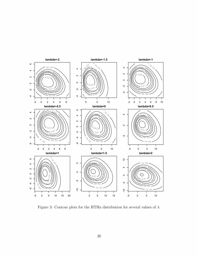
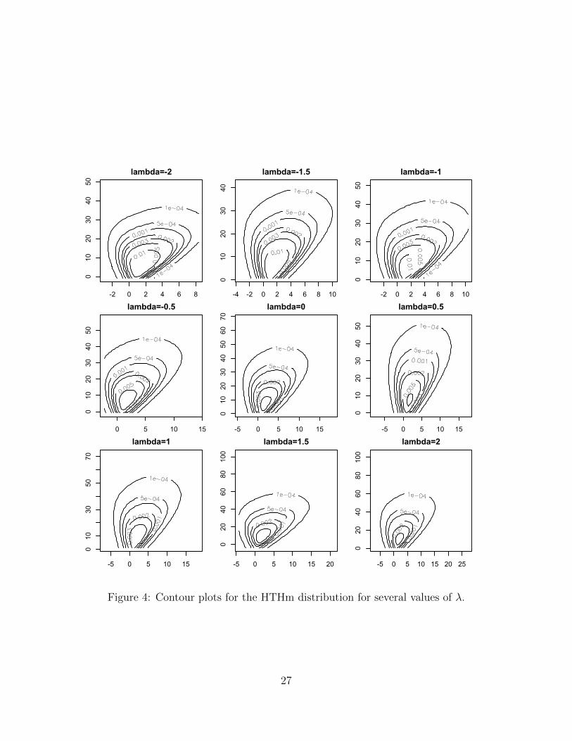
A Convexity of the HTH Distribution

From Section 5, convexity of the HTH distribution cannot be proven for −(p + q)/2 < λ <(p+ q + 1)/2. In this appendix, we give examples of contours generated for λ in this range.Note that when there is no skewness, the contours will be elliptical and thus convex. As ofyet, we have not be able to generate a situation with −(p+ q)/2 < λ < (p+ q + 1)/2 wherethe contours are not convex. For example, we consider data generated with p = 2, q = 1 and

µ =

(11

)Σ =

(1.5 0.30.3 2

)ω = 2 Λ =

(9−5

).

We plot the contours of the distribution for −2 < λ < 2 (Figure 3). Similarly, we considerdata generated with p = 2, q = 2 and

µ =

(11

)Σ =

(1.5 0.30.3 2

)ω = 2 Λ =

(−1 93 9

).

The contours of the distribution are plotted for −2 < λ < 2 (Figure 4). In both examplesthat all of the contours are convex. In our experience, this is typical.

25

lambda=-2

X1

X2

-2 0 2 4 6 8

-4-2

02

46

lambda=-1.5

X1

X2

0 5 10

-4-2

02

4

lambda=-1

X1

X2

-2 0 2 4 6 8 10

-4-2

02

4

lambda=-0.5

X1

X2

-2 0 2 4 6 8

-6-4

-20

24

lambda=0

X1

X2

0 5 10

-6-4

-20

24

6

lambda=0.5

X1

X2

-5 0 5 10

-50

5

lambda=1

X1

X2

-5 0 5 10 15 20

-6-4

-20

24

6

lambda=1.5

X1

X2

0 5 10 15

-10

-50

5

lambda=2

X1

X2

-5 0 5 10

-10

-50

510

Figure 3: Contour plots for the HTHu distribution for several values of λ.

26

lambda=-2

X1

X2

-2 0 2 4 6 8

010

2030

4050

lambda=-1.5

X1

X2

-4 -2 0 2 4 6 8 10

010

2030

40

lambda=-1

X1

X2

-2 0 2 4 6 8 10

010

2030

4050

lambda=-0.5

X1

X2

0 5 10 15

010

2030

4050

lambda=0

X1

X2

-5 0 5 10 15

010

2030

4050

6070

lambda=0.5

X1

X2

-5 0 5 10 15

010

2030

4050

lambda=1

X1

X2

-5 0 5 10 15

010

3050

70

lambda=1.5

X1

X2

-5 0 5 10 15 20

020

4060

80100

lambda=2

X1

X2

-5 0 5 10 15 20 25

020

4060

80100

Figure 4: Contour plots for the HTHm distribution for several values of λ.

27