lecture notes on quantum information and...
TRANSCRIPT

Draft for Internal Circulations:v1: Fall Semester, 2012; v2: Fall Semester, 2013;
v3: Fall Semester, 2014;
Lecture Notes on
Quantum Information and Computation
Yong Zhang1
School of Physics and Technology, Wuhan University
(Fall 2014)
Abstract
These lectures notes are written for both advanced undergraduate studentsand first-year graduate students in the School of Physics and Technology,University Wuhan. They are mainly based on both online lecture notes ofJohn Preskill from Caltech and the standard textbook of Michael Nielsen andIssac Chuang, so I do not claim any originality. I do take the full responsibilityfor all kinds of typos or errors (besides errors in English writing), and pleaselet me know of them.
* The second version of these notes are typeset by
Yi Peng2
Undergraduate student (Id: 2010301020027),
Participant in the Fall semester, 2013.
* The third version of these notes are typeset by
Kun Zhang3
Graduate student (Id: 2013202020002),
Participant in the Fall semester, 2012-2013-2014.

Draft for Internal Circulations:v3: Fall Semester, 2014
Acknowledgements
I thank all participants in class including advanced undergraduate students,first-year graduate students and French students for their patience and persis-tence and for their various enlightening questions. I especially thank studentswho are willing to devote their precious time to the typewriting of these lecturenotes in Latex.
Main References to Lecture Notes
* [Preskill] John Preskill (Caltech): online lecture notes on QIC (1997-present),
http://www.theory.caltech.edu/∼preskill/ph229/
http://www.theory.caltech.edu/∼preskill/ph229/♯lecture
* [Nilesen & Chuang] Michael A. Nielsen and Isaac L. Chuang,
Quantum Computation and Quantum Information (Cambridge, 2000&2010)
* [KLM] Phillip Kaye, Raymond Laflamme and Michele Mosca,
An Introduction to Quantum Computing (Oxford, 2007).
* [Zhang] Yong-De Zhang (University of Science & Technology of China),
Principles of Quantum Information Physics (in Chinese) (Science Press, 2009).
Main References to Homeworks
* [Preskill] John Preskill (Caltech): online lecture notes on QIC (1997-present),
http://www.theory.caltech.edu/∼preskill/ph229/♯lecture
2

To our parents and our teachers!
To be the best researcher is to be the best person first of all:
Respect and listen to our parents and our teachers always!
3

This course focuses on fundamental principles of quantum mechanics.
The aim of this course is to study the simulation of both quantum field theoryand quantum gravity on a quantum computer.
4
Contents
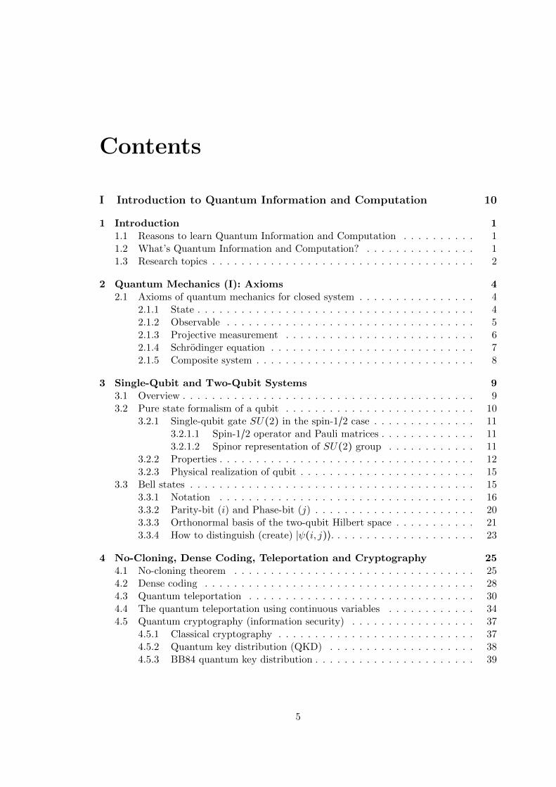
I Introduction to Quantum Information and Computation 10
1 Introduction 11.1 Reasons to learn Quantum Information and Computation . . . . . . . . . . 11.2 What’s Quantum Information and Computation? . . . . . . . . . . . . . . . 11.3 Research topics . . . . . . . . . . . . . . . . . . . . . . . . . . . . . . . . . . . . 2
2 Quantum Mechanics (I): Axioms 42.1 Axioms of quantum mechanics for closed system . . . . . . . . . . . . . . . . 4
2.1.1 State . . . . . . . . . . . . . . . . . . . . . . . . . . . . . . . . . . . . . . 42.1.2 Observable . . . . . . . . . . . . . . . . . . . . . . . . . . . . . . . . . . 52.1.3 Projective measurement . . . . . . . . . . . . . . . . . . . . . . . . . . 62.1.4 Schrodinger equation . . . . . . . . . . . . . . . . . . . . . . . . . . . . 72.1.5 Composite system . . . . . . . . . . . . . . . . . . . . . . . . . . . . . . 8
3 Single-Qubit and Two-Qubit Systems 93.1 Overview . . . . . . . . . . . . . . . . . . . . . . . . . . . . . . . . . . . . . . . . 93.2 Pure state formalism of a qubit . . . . . . . . . . . . . . . . . . . . . . . . . . 10
3.2.1 Single-qubit gate SU(2) in the spin-1/2 case . . . . . . . . . . . . . . 113.2.1.1 Spin-1/2 operator and Pauli matrices . . . . . . . . . . . . . 113.2.1.2 Spinor representation of SU(2) group . . . . . . . . . . . . 11
3.2.2 Properties . . . . . . . . . . . . . . . . . . . . . . . . . . . . . . . . . . . 123.2.3 Physical realization of qubit . . . . . . . . . . . . . . . . . . . . . . . . 15
3.3 Bell states . . . . . . . . . . . . . . . . . . . . . . . . . . . . . . . . . . . . . . . 153.3.1 Notation . . . . . . . . . . . . . . . . . . . . . . . . . . . . . . . . . . . 163.3.2 Parity-bit (i) and Phase-bit (j) . . . . . . . . . . . . . . . . . . . . . . 203.3.3 Orthonormal basis of the two-qubit Hilbert space . . . . . . . . . . . 213.3.4 How to distinguish (create) ∣ψ(i, j)⟩. . . . . . . . . . . . . . . . . . . . 23
4 No-Cloning, Dense Coding, Teleportation and Cryptography 254.1 No-cloning theorem . . . . . . . . . . . . . . . . . . . . . . . . . . . . . . . . . 254.2 Dense coding . . . . . . . . . . . . . . . . . . . . . . . . . . . . . . . . . . . . . 284.3 Quantum teleportation . . . . . . . . . . . . . . . . . . . . . . . . . . . . . . . 304.4 The quantum teleportation using continuous variables . . . . . . . . . . . . 344.5 Quantum cryptography (information security) . . . . . . . . . . . . . . . . . 37
4.5.1 Classical cryptography . . . . . . . . . . . . . . . . . . . . . . . . . . . 374.5.2 Quantum key distribution (QKD) . . . . . . . . . . . . . . . . . . . . 384.5.3 BB84 quantum key distribution . . . . . . . . . . . . . . . . . . . . . . 39
5

5 Bell Inequalities 415.1 Einstein’s quantum mechanics: local hidden variable theory (LHV) . . . . . 41
5.1.1 What hidden variable (HV) theory? . . . . . . . . . . . . . . . . . . . 415.1.2 What local theory? . . . . . . . . . . . . . . . . . . . . . . . . . . . . . 425.1.3 The rule to justify the rightful theory . . . . . . . . . . . . . . . . . . 42
5.2 Bell’s inequality in the local hidden variable theory . . . . . . . . . . . . . . 425.3 Bell’s inequality in quantum mechanics . . . . . . . . . . . . . . . . . . . . . 445.4 The CHSH inequality . . . . . . . . . . . . . . . . . . . . . . . . . . . . . . . . 485.5 Hints for the violation of the Bell inequality . . . . . . . . . . . . . . . . . . . 505.6 Hardy’s theorem . . . . . . . . . . . . . . . . . . . . . . . . . . . . . . . . . . . 505.7 The GHZ theorem . . . . . . . . . . . . . . . . . . . . . . . . . . . . . . . . . . 55
II Quantum Computing and Quantum Algorithm 57
6 Classical Circuit and Quantum Circuit 586.1 Classical circuit . . . . . . . . . . . . . . . . . . . . . . . . . . . . . . . . . . . . 58
6.1.1 Universal gate set . . . . . . . . . . . . . . . . . . . . . . . . . . . . . . 596.1.1.1 Elementary logical gates . . . . . . . . . . . . . . . . . . . . 596.1.1.2 Universal gate set . . . . . . . . . . . . . . . . . . . . . . . . 60
6.2 Reversible classical computation . . . . . . . . . . . . . . . . . . . . . . . . . . 606.2.1 Irreversible computation . . . . . . . . . . . . . . . . . . . . . . . . . . 606.2.2 Classical reversible gate . . . . . . . . . . . . . . . . . . . . . . . . . . 616.2.3 Three-bit Toffoli gate . . . . . . . . . . . . . . . . . . . . . . . . . . . . 626.2.4 Three-bit Fredkin gate . . . . . . . . . . . . . . . . . . . . . . . . . . . 63
6.3 The construction of an n-bit Toffoli gate using the 3-bit Toffoli gate . . . . 646.4 Quantum circuit model . . . . . . . . . . . . . . . . . . . . . . . . . . . . . . . 66
6.4.1 Definition of quantum circuit . . . . . . . . . . . . . . . . . . . . . . . 676.4.2 One-qubit gates . . . . . . . . . . . . . . . . . . . . . . . . . . . . . . . 676.4.3 Hadamard gate: HHH . . . . . . . . . . . . . . . . . . . . . . . . . . . . . 716.4.4 Controlled two-qubit gates and controlled three-qubit gates . . . . . 74
6.4.4.1 CNOT gate . . . . . . . . . . . . . . . . . . . . . . . . . . . . 756.4.4.2 Quantum Toffoli gate and Fredkin gate . . . . . . . . . . . 79
6.4.5 Quantum circuit model of Bell states . . . . . . . . . . . . . . . . . . 796.4.6 Quantum circuit model of GHZ states . . . . . . . . . . . . . . . . . . 81
6.5 Universal quantum computation . . . . . . . . . . . . . . . . . . . . . . . . . . 856.5.1 Quantum universal gate set . . . . . . . . . . . . . . . . . . . . . . . . 856.5.2 Universal quantum gate set of two-qubit gates . . . . . . . . . . . . . 866.5.3 Deutsch’s gate is a universal quantum gate . . . . . . . . . . . . . . . 89
7 Quantum Algorithms 917.1 Classical and quantum algorithm . . . . . . . . . . . . . . . . . . . . . . . . . 917.2 Oracle model . . . . . . . . . . . . . . . . . . . . . . . . . . . . . . . . . . . . . 927.3 Deutsch’s algorithm . . . . . . . . . . . . . . . . . . . . . . . . . . . . . . . . . 93
7.3.1 Definitions . . . . . . . . . . . . . . . . . . . . . . . . . . . . . . . . . . 937.3.2 Classical algorithm . . . . . . . . . . . . . . . . . . . . . . . . . . . . . 947.3.3 Deutsch’s problem . . . . . . . . . . . . . . . . . . . . . . . . . . . . . . 947.3.4 Phase kick-back . . . . . . . . . . . . . . . . . . . . . . . . . . . . . . . 947.3.5 Deutsch’s algorithm . . . . . . . . . . . . . . . . . . . . . . . . . . . . . 96
6

7.4 Deutsch-Jozsa’s algorithm . . . . . . . . . . . . . . . . . . . . . . . . . . . . . 977.4.1 Constant and balanced function in n-qubit . . . . . . . . . . . . . . . 977.4.2 Constant or balanced function? . . . . . . . . . . . . . . . . . . . . . . 977.4.3 Notation and lemma . . . . . . . . . . . . . . . . . . . . . . . . . . . . 987.4.4 Deutsch-Jozsa’s algorithm . . . . . . . . . . . . . . . . . . . . . . . . . 99
7.5 Bernstein-Vazirani’s algorithm . . . . . . . . . . . . . . . . . . . . . . . . . . . 1017.6 Simon’s algorithm . . . . . . . . . . . . . . . . . . . . . . . . . . . . . . . . . . 1027.7 Grover’s algorithm . . . . . . . . . . . . . . . . . . . . . . . . . . . . . . . . . . 102
7.7.1 Overview of the problem . . . . . . . . . . . . . . . . . . . . . . . . . . 1037.7.2 Grover’s algorithm . . . . . . . . . . . . . . . . . . . . . . . . . . . . . 1037.7.3 Example: N = 4 . . . . . . . . . . . . . . . . . . . . . . . . . . . . . . . 1067.7.4 Quantum circuit model of Grover’s algorithm . . . . . . . . . . . . . 108
III Density Matrix and Quantum Entanglement 111
8 Quantum Mechanics (II): Density Matrix 1128.1 Density matrix as state of quantum open system . . . . . . . . . . . . . . . . 112
8.1.1 State ensemble formalism of density matrix . . . . . . . . . . . . . . 1138.1.2 Operator formalism of density matrix . . . . . . . . . . . . . . . . . . 1158.1.3 Reduced density matrix (State for subsystem) . . . . . . . . . . . . 116
8.2 Mixed state formalism of a qubit . . . . . . . . . . . . . . . . . . . . . . . . . 1188.2.1 Why polarization vector? . . . . . . . . . . . . . . . . . . . . . . . . . 1198.2.2 Pure state and mixed state in two-dimensional Hilbert space H2 . . 120
8.3 Convexity of density matrix . . . . . . . . . . . . . . . . . . . . . . . . . . . . 1228.4 Two-qubit system and its subsystem . . . . . . . . . . . . . . . . . . . . . . . 123
8.4.1 Example: EPR pair (Bell state) . . . . . . . . . . . . . . . . . . . . . 1238.4.2 Maximally entangled two-qubit pure states . . . . . . . . . . . . . . . 1248.4.3 Monogamy of maximal entanglement . . . . . . . . . . . . . . . . . . 125
9 Schmidt Decomposition, Purification and GHJW Theorem 1279.1 Introduction . . . . . . . . . . . . . . . . . . . . . . . . . . . . . . . . . . . . . . 1279.2 Schmidt decomposition and quantum entanglement . . . . . . . . . . . . . . 127
9.2.1 Schmidt decomposition . . . . . . . . . . . . . . . . . . . . . . . . . . . 1279.2.2 Quantum entanglement . . . . . . . . . . . . . . . . . . . . . . . . . . . 1289.2.3 Proof for the theorem of the Schmidt decomposition . . . . . . . . . 129
9.3 Example for the Schmidt decomposition . . . . . . . . . . . . . . . . . . . . . 1309.4 The purification theorem and GHJW theorem . . . . . . . . . . . . . . . . . 134
9.4.1 Purification . . . . . . . . . . . . . . . . . . . . . . . . . . . . . . . . . . 1349.4.2 The GHJW theorem . . . . . . . . . . . . . . . . . . . . . . . . . . . . 135
9.5 Information is physics . . . . . . . . . . . . . . . . . . . . . . . . . . . . . . . . 136
10 Mixed State Entanglement and Multi-partite Entanglement 13910.1 Bipartite mixed state entanglement . . . . . . . . . . . . . . . . . . . . . . . . 139
10.1.1 Separability . . . . . . . . . . . . . . . . . . . . . . . . . . . . . . . . . . 13910.1.1.1 Bipartite pure states . . . . . . . . . . . . . . . . . . . . . . . 13910.1.1.2 Bipartite mixed state . . . . . . . . . . . . . . . . . . . . . . 140
10.1.2 Quantum bipartite entanglement . . . . . . . . . . . . . . . . . . . . . 14010.1.3 Positive-partial transpose (PPT) criterion for quantum bipartite
separability . . . . . . . . . . . . . . . . . . . . . . . . . . . . . . . . . . 141
7

10.1.4 Example: the Werner state and the PPT criterion . . . . . . . . . . 14110.1.5 Example: the Werner state and the CHSH inequality . . . . . . . . . 145
10.2 Multi-partite entanglement . . . . . . . . . . . . . . . . . . . . . . . . . . . . . 14610.2.1 Definition . . . . . . . . . . . . . . . . . . . . . . . . . . . . . . . . . . . 14610.2.2 The GHZ state . . . . . . . . . . . . . . . . . . . . . . . . . . . . . . . . 14710.2.3 Properties of GHZ states . . . . . . . . . . . . . . . . . . . . . . . . . . 150
IV Quantum Open System and Quantum Error Correction Codes 152
11 Quantum Mechanics (III): Quantum Open System 15311.1 Introduction . . . . . . . . . . . . . . . . . . . . . . . . . . . . . . . . . . . . . . 154
11.1.1 Why we talk about quantum open system . . . . . . . . . . . . . . . 15411.1.2 Closed system and open system . . . . . . . . . . . . . . . . . . . . . . 154
11.2 Projective measurement . . . . . . . . . . . . . . . . . . . . . . . . . . . . . . . 15411.3 General measurement theory . . . . . . . . . . . . . . . . . . . . . . . . . . . . 15611.4 Definition of POVM . . . . . . . . . . . . . . . . . . . . . . . . . . . . . . . . . 15711.5 More on POVM . . . . . . . . . . . . . . . . . . . . . . . . . . . . . . . . . . . 159
11.5.1 Dimensional analysis . . . . . . . . . . . . . . . . . . . . . . . . . . . . 15911.5.2 POVM on subsystem can be viewed as projective measurements on
the entire system . . . . . . . . . . . . . . . . . . . . . . . . . . . . . . 15911.5.3 Tensor product realization of POVM . . . . . . . . . . . . . . . . . . 160
11.5.3.1 Operator formula of FFF a . . . . . . . . . . . . . . . . . . . . . 16011.5.3.2 Matrix formalism of Fa . . . . . . . . . . . . . . . . . . . . . 16011.5.3.3 The properties of FFFA
a . . . . . . . . . . . . . . . . . . . . . . 16111.5.3.4 Example . . . . . . . . . . . . . . . . . . . . . . . . . . . . . . 161
11.5.4 Direct-sum realization of POVM . . . . . . . . . . . . . . . . . . . . . 16311.5.5 POVM as quantum operation (superoperator) . . . . . . . . . . . . . 163
11.6 Quantum operation (superoperator) . . . . . . . . . . . . . . . . . . . . . . . 16311.6.1 Definition of the superoperator . . . . . . . . . . . . . . . . . . . . . . 16311.6.2 The wonderful theorem . . . . . . . . . . . . . . . . . . . . . . . . . . . 16411.6.3 The CPTP mapping . . . . . . . . . . . . . . . . . . . . . . . . . . . . 16511.6.4 The Kraus representation . . . . . . . . . . . . . . . . . . . . . . . . . 16511.6.5 The Stinespring representation . . . . . . . . . . . . . . . . . . . . . . 16611.6.6 Remarks on quantum operation . . . . . . . . . . . . . . . . . . . . . . 167
11.7 Quantum channel . . . . . . . . . . . . . . . . . . . . . . . . . . . . . . . . . . 16711.7.1 The bit-flip channel . . . . . . . . . . . . . . . . . . . . . . . . . . . . . 16711.7.2 The phase-flip channel . . . . . . . . . . . . . . . . . . . . . . . . . . . 16911.7.3 Depolarizing channel . . . . . . . . . . . . . . . . . . . . . . . . . . . . 16911.7.4 The phase-damping channel . . . . . . . . . . . . . . . . . . . . . . . . 17011.7.5 The amplitude-damping channel . . . . . . . . . . . . . . . . . . . . . 171
11.8 The master equation . . . . . . . . . . . . . . . . . . . . . . . . . . . . . . . . . 172
12 Notes on Finite Group Theory 174
13 Notes on Stabilizer Formalism of Quantum Error Correction Codes 175
8
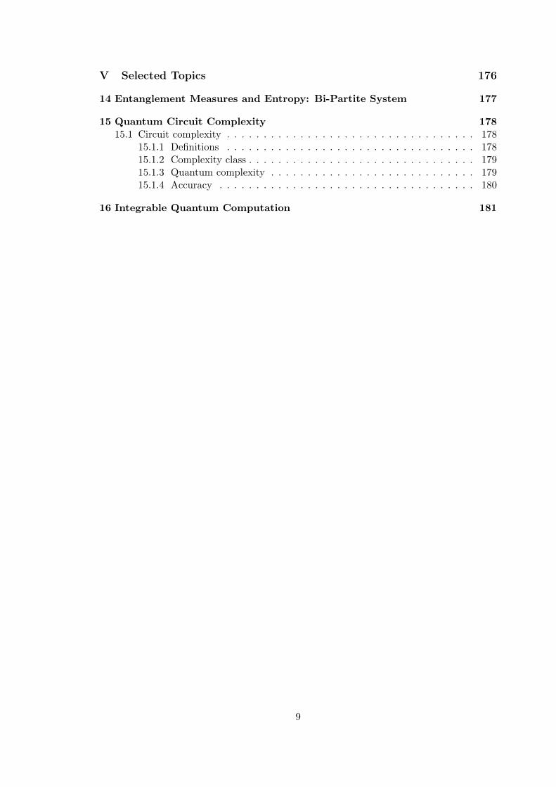
V Selected Topics 176
14 Entanglement Measures and Entropy: Bi-Partite System 177
15 Quantum Circuit Complexity 17815.1 Circuit complexity . . . . . . . . . . . . . . . . . . . . . . . . . . . . . . . . . . 178
15.1.1 Definitions . . . . . . . . . . . . . . . . . . . . . . . . . . . . . . . . . . 17815.1.2 Complexity class . . . . . . . . . . . . . . . . . . . . . . . . . . . . . . . 17915.1.3 Quantum complexity . . . . . . . . . . . . . . . . . . . . . . . . . . . . 17915.1.4 Accuracy . . . . . . . . . . . . . . . . . . . . . . . . . . . . . . . . . . . 180
16 Integrable Quantum Computation 181
9

Part I
Introduction to QuantumInformation and Computation
10

Chapter 1
Introduction
References:
[Preskill] Chapter 1: Introduction and overview;
[Nielsen & Chuang] Chapter 1: Introduction and overview.
1.1 Reasons to learn Quantum Information and Computa-tion
For an advanced undergraduate major in physics, he or she has to learn Quantum Infor-mation and Computation, because
• Quantum Information and Computation can be seen as a new type of advancedQuantum Mechanics between Quantum Mechanics and Quantum Field Theory;
• Quantum Information and Computation represents a further development of Quan-tum Mechanics;
• what Quantum Information and Computation focuses is the logic of the QuantumMechanics.
The reason for a graduate student major in physics to learn Quantum Information andComputation is that
• if a graduate want to do great in modern theoretical physics (especially in QuantumField Theory or High Energy Physics or Condensed Matter Physics), he or she hasto understand Quantum Information and Computation very well, because he or shemust understand Modern Quantum Mechanics which is represented by QuantumInformation and Computation.
1.2 What’s Quantum Information and Computation?
There are many different opinions about this question:
• In Michael A. Nielsen and Isaac L. Chuang’s opinion,
⋯ Quantum computation and quantum information is the study of theinformation process tasks that can be accomplished using quantum me-chanical systems (or using fundamentals of quantum mechanics) ⋯
1
• According to Rolf Landauer (1961),
⋯ Information is physical ⋯
which says that information is something that is encoded in the states of physicalsystems.
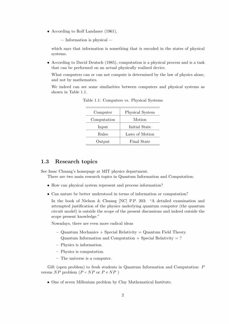
• According to David Deutsch (1985), computation is a physical process and is a taskthat can be performed on an actual physically realized device.
What computers can or can not compute is determined by the law of physics alone,and not by mathematics.
We indeed can see some similarities between computers and physical systems asshown in Table 1.1.
Table 1.1: Computers vs. Physical Systems
Computer Physical System
Computation Motion
Input Initial State
Rules Laws of Motion
Output Final State
1.3 Research topics
See Issac Chuang’s homepage at MIT physics department.There are two main research topics in Quantum Information and Computation:
• How can physical system represent and process information?
• Can nature be better understood in terms of information or computation?
In the book of Nielson & Chuang [NC] P.P. 203: “A detailed examination andattempted justification of the physics underlying quantum computer (the quantumcircuit model) is outside the scope of the present discussions and indeed outside thescope present knowledge.”
Nowadays, there are even more radical ideas
– Quantum Mechanics + Special Relativity = Quantum Field Theory.
Quantum Information and Computation + Special Relativity = ?
– Physics is information.
– Physics is computation.
– The universe is a computer.
Gift (open problem) to fresh students in Quantum Information and Computation: Pversus NP problem (P = NP or P ≠ NP )
• One of seven Millenium problem by Clay Mathematical Institute.
2

• Experts intend to believe P ≠ NP or P ⊂ NP , but no proof up to now.
• P ≠ NP means there may exist problems which can not be solved efficiently, and itmay put a new constraint on Nature like the light speed or the uncertainty principle.
• Google & Wiki for details
3

Chapter 2
Quantum Mechanics (I): Axioms
For those who are not shocked when they first come across quantum theorycan not possibly have understood it.
—Niels Bohr
I think I can safely say that nobody understands quantum mechanics.
—Richard Feynman
Quantum mechanics: Real black magic calculus
—Albert Einstein
References:
[Preskill] Chapter 2: Foundations I: states and ensembles;
[Nielsen & Chuang] Chapter 2: Introduction to quantum mechanics.
2.1 Axioms of quantum mechanics for closed system
Principles of quantum mechanics can be classified into two parts: the static part includes“States” and “Observables, and the dynamic part includes “Evolution” and “Measure-ment”.
When we talk about axioms of quantum mechanics, we introduce axioms for quantumclosed systems and axioms for quantum open systems respectively, see the following table.The axioms for quantum open system will be discussed in detail in Chapter 11.
2.1.1 State
Axiom 2.1.1. A state ∣ψ⟩ or a ray eiα ∣ψ⟩ , from the Hilbert space H , can make acomplete description of a physical system (with no hidden variable).
Ray is an equivalent class of vectors, where global phase has no physical meaning. But,notice that the relative phase however is of physical significance. For example, the s-tate vector ∣0⟩ + ∣1⟩ is physically different from ∣0⟩ + eiα∣1⟩ with eiα ≠ 1. Note that thesuperposition principle is defined only for state vectors, not for state rays.
4

Axioms of Quantum Mechanics
Closed Systems Open Systems
Eg: the entire universe Eg: subsystems of a composite system
Space Hilbert space H
Statepure state vector ∣φ⟩ ∈ H
density matrix (operator) ρpure state ray eiα ∣φ⟩ ∈ H called mixed state
Observableself-adjoint operator A = ∑n anP n
with an ⊂ R and P n being orthogonal projections
Measurement
projective measurement general measurement
(orthogonal) (non-orthogonal)
⟨A⟩ = ⟨φ∣A ∣φ⟩ ⟨A⟩ = tr(Aρ)
Dynamicsunitary evolution non-unitary evolution via superoperator
Eg: ih ddt
∣φ(t)⟩ =H ∣φ(t)⟩ Eg: ih ddtρ(t) = [H,ρ(t)]
2.1.2 Observable
An observable in physics is a property of a physical system that can be measured.
Axiom 2.1.2. With every observable, there exists an associated linear, self-adjoint oper-ator A, which acts in the Hilbert space H ,
A† =A⇐⇒ ⟨ψ∣Aφ⟩ = ⟨Aψ∣φ⟩ , with ∣ψ⟩ , ∣φ⟩ ∈H . (2.1.1)
Let an be one of the eigenvalues of A and ∣an⟩ is the associated eigenvector,
A ∣an⟩ = an ∣an⟩ . (2.1.2)
All the eigenvalues an of A are real, while the eigenvectors ∣an⟩ form a complete or-thogonal basis of the Hilbert space H .It would be easy to prove that the eigenvalues of the observable A is real, and the itseigenvectors are orthogonal.
Proof.
(i) The eigenvalues of the observable A are real.
A ∣an⟩ = an ∣an⟩( ⟨an∣A ∣an⟩ )
∗ = ⟨an∣A† ∣an⟩ = ⟨an∣A ∣an⟩ ⇒ a∗n = an, (2.1.3)
i.e., an is real.
(ii) The eigenvectors of the observable A are orthogonal.
• In the case of two eigenvectors with different eigenvalues, namely
A ∣ak⟩ = ak ∣ak⟩A ∣a`⟩ = a` ∣a`⟩
(2.1.4)
with k≠` and ak≠an. Therefore,
⟨ak∣A ∣a`⟩ = a` ⟨ak ∣a`⟩⟨ak∣A ∣a`⟩ = ak ⟨ak ∣a`⟩
⇒ (ak − a`) ⟨ak ∣a`⟩ = 0 ⇒ ⟨ak ∣a`⟩ = 0. (2.1.5)
5

• In the circumstance of degeneration, namely, there are at least two mutuallyindependent eigenvectors of A, but with the same eigenvalue. The set of al-l these eigenvectors of A associated with the specific eigenvalue would span asubspace of the Hilbert space H . Thus, we can employ the Schmidt orthogonal-ization process, to make an orthogonal basis for such a subspace, with the basisvectors still being the eigenvectors of the observable A and the correspondingeigenvalue unchanged.
The spectral theorem. We can define the orthogonal projection operators P n onto thesubspace associated with the eigenvalue an of the Hilbert space H , namely
Han ∶=A ∣φ⟩ = an ∣φ⟩ ∣ ∀ ∣φ⟩ ∈H , (2.1.6)
as
P n =Degeneracy
∑k=1
∣a(k)n ⟩ ⟨a(k)n ∣ , (2.1.7)
with ∣a(k)n ⟩ ∣ k = 1, . . . ,Degeneracy be an orthonormal basis for the subspace Han . It’s
easy to see that⎧⎪⎪⎪⎨⎪⎪⎪⎩
P †n = P n,
P 2n = P n,
P nPm = 0, if n ≠ m.
(2.1.8)
Hence, we can expand the operator A as
A =∑n
anP n, (2.1.9)
which is the spectral theorem.
2.1.3 Projective measurement
Axiom 2.1.3. For an observable A with eigenvalues an and eigenvectors ∣an⟩, given thesystem is in the state ∣ψ⟩, the probability of obtaining an (in the non-degeneration case)as the outcome of the measurement of A is
Prob(an) = ∣ ⟨an ∣ψ⟩ ∣2. (2.1.10)
And the expectation value (mean value) of the observable A would be
⟨A⟩ = ⟨ψ∣A ∣ψ⟩⟨ψ ∣ψ⟩
. (2.1.11)
After the measurement, the system is left in the state within the subspace correspondingto the eigenvalue an (the so called wavepacket collapse).
The name “ projection measurement” is evident as we shall see. For example, we cansee that the operator P n = ∣an⟩ ⟨an∣, itself is a self-adjoint operator, which has the meanvalue,
⟨ψ∣P n ∣ψ⟩ = ⟨ψ∣ ( ∣an⟩ ⟨an∣ ) ∣ψ⟩= ⟨ψ ∣an⟩ ⟨an ∣ψ⟩= ∣ ⟨an ∣ψ⟩ ∣2 = Prob(an), (2.1.12)
6
where ∣ψ⟩ is the normalized state vector of the physical system.
∣ψ⟩Pn=∣an⟩⟨an∣ÐÐÐÐÐÐÐ→ P n ∣ψ⟩√
⟨ψ∣P n ∣ψ⟩= ∣an⟩
⟨an ∣ψ⟩∣ ⟨an ∣ψ⟩ ∣
, (2.1.13)
which is the post-measurement state.
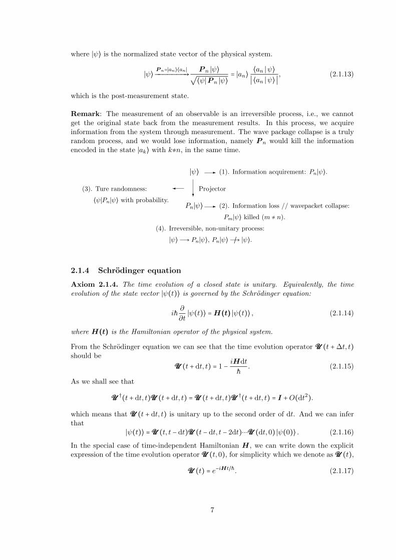
Remark: The measurement of an observable is an irreversible process, i.e., we cannotget the original state back from the measurement results. In this process, we acquireinformation from the system through measurement. The wave package collapse is a trulyrandom process, and we would lose information, namely P n would kill the informationencoded in the state ∣ak⟩ with k≠n, in the same time.
∣ψ⟩
?
Pn∣ψ⟩
- (1). Information acquirement: Pn∣ψ⟩.
- (2). Information loss // wavepacket collapse:
Pm∣ψ⟩ killed (m ≠ n).
Projector(3). Ture randomness:
⟨ψ∣Pn∣ψ⟩ with probability.
/(4). Irreversible, non-unitary process:
∣ψ⟩Ð→ Pn∣ψ⟩, Pn∣ψ⟩Ð→ ∣ψ⟩.
2.1.4 Schrodinger equation
Axiom 2.1.4. The time evolution of a closed state is unitary. Equivalently, the timeevolution of the state vector ∣ψ(t)⟩ is governed by the Schrodinger equation:
ih∂
∂t∣ψ(t)⟩ =H(t) ∣ψ(t)⟩ , (2.1.14)
where H(t) is the Hamiltonian operator of the physical system.
From the Schrodinger equation we can see that the time evolution operator UUU (t +∆t, t)should be
UUU (t + dt, t) = 1 − iHdt
h. (2.1.15)
As we shall see that
UUU †(t + dt, t)UUU (t + dt, t) =UUU (t + dt, t)UUU †(t + dt, t) = I +O(dt2).
which means that UUU (t + dt, t) is unitary up to the second order of dt. And we can inferthat
∣ψ(t)⟩ =UUU (t, t − dt)UUU (t − dt, t − 2dt)⋯UUU (dt,0) ∣ψ(0)⟩ . (2.1.16)
In the special case of time-independent Hamiltonian H, we can write down the explicitexpression of the time evolution operator UUU (t,0), for simplicity which we denote as UUU (t),
UUU (t) = e−iHt/h. (2.1.17)
7

In the case of time-dependent Hamiltonian H(t), we have to use the Dyson’s formula
UUU (t) = I +∞
∑n=1
1
n!(− ih)n
∫t
0dtn∫
t
0dtn−1⋯∫
t
0dt1H(tn)H(tn−1)⋯H(t1)
´¹¹¹¹¹¹¹¹¹¹¹¹¹¹¹¹¹¹¹¹¹¹¹¹¹¹¹¹¹¹¹¹¹¹¹¹¹¹¹¹¹¹¹¹¹¹¹¹¹¹¹¹¹¹¹¹¹¹¹¹¹¹¹¹¹¹¹¹¹¹¹¸¹¹¹¹¹¹¹¹¹¹¹¹¹¹¹¹¹¹¹¹¹¹¹¹¹¹¹¹¹¹¹¹¹¹¹¹¹¹¹¹¹¹¹¹¹¹¹¹¹¹¹¹¹¹¹¹¹¹¹¹¹¹¹¹¹¹¹¹¹¹¹¹¶tn>tn−1>⋯>t1
, (2.1.18)
see Google & Wiki for more details.
Remark: Why is the Schrodinger equation linear? Why is the time evolution unitary,but different with measurement which is a non-unitary process? Why we have two distinctevolutions in quantum mechanics?
2.1.5 Composite system
For system A, ∣ψ⟩A ∈ HA, and system B, ∣ϕ⟩B ∈ HB, the composite system of system A andsystem B is described by the tensor product of Hilbert spaces, i.e., ∣ψ⟩A⊗ ∣ϕ⟩B ∈ HA⊗HB.
8

Chapter 3
Single-Qubit and Two-QubitSystems
References:
[Preskill]Chapter 2: Foundations I: states and ensembles;
[Preskill] Chapter 4: Quantum entanglement;
[Nielsen & Chuang] Chapter 1: Introduction and overview;
[Nielsen & Chuang] Chapter 2: Introduction to quantum mechanics.
3.1 Overview
Classical computation vs. Quantum Computation
Classical Computation Quantum Computation
Information unit bit qubit
Operation gate quantum gate
For Classical Computation, the basic units that store the information and are manipulatedare the bits. The “tool” that can manipulate bits are the so-called classical logic gate.
• bit: the short name of “binary digit”, which can only take the value of 0 or 1.
• gate:
gate one-bit gate NOTtwo-bit gate AND, OR, . . .
NOT gate: a in mod 2. AND gate: a ∧ b ≡ a ⋅ b, OR gate: a ∨ b ≡ a⊕ b in mod 2.
While for Quantum computation, the counterpart for bit should be qubit, and for classicallogic gates are quantum gates.
• qubit: the short name of “quantum bit”, which can be considered as a state vectorin the two-dimensional Hilbert space H2:
(αβ) = α ∣0⟩ + β ∣1⟩ , with ∣α∣2 + ∣β∣2 = 1, α, β ∈ C, (3.1.1)
9

where ∣0⟩ could mean “spin up” and for ∣1⟩ mean “spin down”, i.e., this is a two-levelphysical system, and the spin-1
2 system is a typical example.
• quantum gate:
quantum gate
⎧⎪⎪⎪⎪⎪⎪⎪⎨⎪⎪⎪⎪⎪⎪⎪⎩
single-qubit gate: (αβ)
SU(2)ÐÐÐ→ (α
′
β′) ,
two-qubit gate: (α1
β1)⊗(α2
β2)
SU(4)ÐÐÐ→ (α
′1
β′1)⊗(α
′2
β′2) .
3.2 Pure state formalism of a qubit
The Hilbert space H2 can be spanned by basis ∣0⟩ , ∣1⟩ , i.e.,
∣ψ⟩ = α ∣0⟩ + β ∣1⟩ = (αβ) , ∀ ∣ψ⟩ ∈H2, with α,β ∈ C and ∣α∣2 + ∣β∣2 = 1.
We may notice that α and β being complex numbers means four real numbers (four degreesof freedom). With the constraint ∣α∣2 + ∣β∣2 = 1, we can cut down the degrees of freedominto three. And, if we ignore the global phase of the state vector (qubit), which has nophysical meaning, then we can reduce the degrees of freedom to be two. Therefore, thestate vector ∣ψ⟩ can be described by two real numbers (θ,ϕ), for example
∣ψ+(θ,ϕ)⟩ ∶= cosθ
2∣0⟩ + eiϕ sin
θ
2∣1⟩ = ( cos θ2
eiϕ sin θ2
) , with 0 ≤ θ < π, and 0 ≤ ϕ < 2π. (3.2.1)
The two real variables (θ,ϕ) can actually determine a unit vector in the three-dimensionalEuclidean R3, namely n = (sin θ cosϕ, sin θ sinϕ, cos θ), as shown in Figure 3.1. And we
x
y
z
ϕ
θn = (sin θ cosϕ, sin θ sinϕ, cos θ)
Figure 3.1: Bloch sphere
shall also see that with n pointing along different directions, namely different values of θand ϕ, the state vectors ∣ψ+(θ,ϕ)⟩ are different:
(1) n = ex = (1,0,0), θ = π2 , ϕ = 0, ⇒ ∣ψ+(π2 ,0)⟩ =
1√2( ∣0⟩ + ∣1⟩ );
(2) n = ey = (0,1,0), θ = π2 , ϕ = π
2 , ⇒ ∣ψ+(π2 ,π2 )⟩ =
1√2( ∣0⟩ + i ∣1⟩ );
(3) n = ez = (0,0,1), θ = 0, ϕ∈[0,2π),⇒ ∣ψ+(0, ϕ)⟩ = ∣0⟩ .
The vector n in three dimensional space is called Bloch vector, and the unit boundaryof the vector set is called Bloch sphere, i.e., ∣n∣ = 1.
10
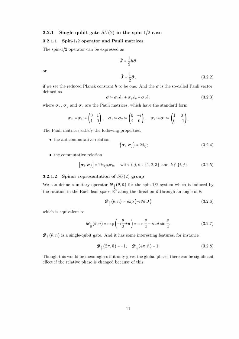
3.2.1 Single-qubit gate SU(2) in the spin-1/2 case
3.2.1.1 Spin-1/2 operator and Pauli matrices
The spin-1/2 operator can be expressed as
J = 1
2hσ
or
J = 1
2σ, (3.2.2)
if we set the reduced Planck constant h to be one. And the σ is the so-called Pauli vector,defined as
σ ∶=σxex +σy ey +σz ez (3.2.3)
where σx, σy and σz are the Pauli matrices, which have the standard form
σx ∶=σ1 ∶= (0 11 0
) , σx ∶=σ2 ∶= (0 −ii 0
) , σz ∶=σ3 ∶= (1 00 −1
) .
The Pauli matrices satisfy the following properties,
• the anticommutative relationσi,σj = 2δij ; (3.2.4)
• the commutative relation
[σi,σj] = 2iεijkσk, with i, j, k ∈ 1,2,3 and k ∉ i, j. (3.2.5)
3.2.1.2 Spinor representation of SU(2) group
We can define a unitary operator DDD 12(θ, n) for the spin-1/2 system which is induced by
the rotation in the Euclidean space R3 along the direction n through an angle of θ:
DDD 12(θ, n) ∶= exp (−iθn⋅J) (3.2.6)
which is equivalent to
DDD 12(θ, n) = exp(−iθ
2n⋅σσσ) = cos
θ
2− in⋅σσσ sin
θ
2. (3.2.7)
DDD 12(θ, n) is a single-qubit gate. And it has some interesting features, for instance
DDD 12(2π, n) = −1, DDD 1
2(4π, n) = 1. (3.2.8)
Though this would be meaningless if it only gives the global phase, there can be significanteffect if the relative phase is changed because of this.
11

3.2.2 Properties
Thm 3.2.2.1. If we define σσσn = σσσ⋅n, then
σσσn ∣ψ+(θ,ϕ)⟩ = ∣ψ+(θ,ϕ)⟩ , with n ∶= (sin θ cosϕ, sin θ sinϕ, cos θ). (3.2.9)
Proof. Let’s firstly express σσσn with the Pauli matrices,
σσσn = sin θ cosϕσσσ1 + sin θ sinϕσσσ2 + cos θσσσ3
= sin θ cosϕ(0 11 0
) + sin θ sinϕ(0 −ii 0
) + cos θ (1 00 −1
)
= ( cos θ sin θ cosϕ − i sin θ sinϕsin θ cosϕ + i sin θ sinϕ − cos θ
)
= ( cos θ sin θ(cosϕ − i sinϕ)sin θ(cosϕ + i sinϕ) − cos θ
) ,
namely
σσσn = ( cos θ sin θe−iϕ
sin θeiϕ − cos θ) . (3.2.10)
Therefore, we can calculate σσσn ∣ψ+(θ,ϕ)⟩ in the following way
σσσn ∣ψ+(θ,ϕ)⟩ = ( cos θ sin θe−iϕ
sin θeiϕ − cos θ)( cos θ2eiϕ sin θ
2
)
=⎛⎝
cos θ cos θ2 + sin θe−iϕeiϕ sin θ2
sin θeiϕ cos θ2 − cos θeiϕ sin θ2
⎞⎠
= ( cos θ2eiϕ sin θ
2
)
= ∣ψ+(θ,ϕ)⟩ . (3.2.11)
There we get E.Q. (3.2.9) proved.
Thm 3.2.2.2.⟨ψ+(θ,ϕ)∣ σσσ⋅m ∣ψ+(θ,ϕ)⟩ = n⋅m, (3.2.12)
with n ∶= (sin θ cosϕ, sin θ sinϕ, cos θ) and m ∈ R3, ∥m∥ = 1.
Proof. In analogy to E.Q.(3.2.10), we can get the expression for σ⋅m:
σσσ⋅m = ( cos θ′ sin θ′e−iϕ′
sin θ′eiϕ′ − cos θ′
) , with m ∶= (sin θ′ cosϕ′, sin θ′ sinϕ′, cos θ′). (3.2.13)
12

Therefore, we can get
⟨ψ+(θ,ϕ)∣ σσσ⋅m ∣ψ+(θ,ϕ)⟩
= (cos θ2 e−iϕ sin θ2)( cos θ′ sin θ′e−iϕ
′
sin θ′eiϕ′ − cos θ′
)( cos θ2eiϕ sin θ
2
)
= (cos θ2 e−iϕ sin θ2)(cos θ2 cos θ′ + sin θ
2 sin θ′ei(ϕ−ϕ′)
cos θ2 sin θ′eiϕ′ − sin θ
2 cos θ′eiϕ)
= cosθ
2( cos
θ
2cos θ′ + sin
θ
2sin θ′ei(ϕ−ϕ
′))
+e−iϕ sinθ
2( cos
θ
2sin θ′eiϕ
′
− sinθ
2cos θ′eiϕ)
= ( cos2 θ
2− sin2 θ
2) cos θ′ + sin
θ
2cos
θ
2sin θ′(ei(ϕ−ϕ
′) + e−i(ϕ−ϕ′))
= cos θ cos θ′ + sin θ sin θ′ cos(ϕ − ϕ′)
= n⋅m, (3.2.14)
where we have used the fact that
n⋅m= (sin θ cosϕ, sin θ sinϕ, cos θ)(sin θ′ cosϕ′, sin θ′ sinϕ′, cos θ′)T
= sin θ sin θ′ cosϕ cosϕ′ + sin θ sin θ′ sinϕ sinϕ′ + cos θ cos θ′
= sin θ sin θ′(cosϕ cosϕ′ + sinϕ sinϕ′) + cos θ cos θ′
= sin θ sin θ′ cos(ϕ − ϕ′) + cos θ cos θ′. (3.2.15)
There, E.Q. (3.2.12) is verified, too.
Remark: For the expression in terms of density matrix, we have
tr (ρ(σσσ⋅m)) = n⋅m, (3.2.16)
where ρ = ∣ψ+(θ,ϕ)⟩⟨ψ+(θ,ϕ)∣.
Thm 3.2.2.3. As we shall know from the definition of ∣ψ+(θ,ϕ)⟩ that
∣0⟩ = ∣↑z⟩ = ∣ψ+(0, ϕ)⟩ , (3.2.17)
then∣ψ+(θ,ϕ)⟩ =DDD(ez→n) ∣0⟩ , with n = (sin θ cosϕ, sin θ sinϕ, cosθ), (3.2.18)
where
DDD(ez→n) ∶= ( cos θ2 −e−iϕ sin θ2
eiϕ sin θ2 cos θ2
) . (3.2.19)
Proof. Firstly, we should realize that
DDD 12(ez→n) =DDD 1
2(θ, n′xy) = exp(−iθ
2σσσ⋅n′xy) , (3.2.20)
where we define
⎧⎪⎪⎨⎪⎪⎩
nxy ∶= (cosϕ, sinϕ,0),n′xy ∶= ( cos(ϕ + π
2 ), sin(ϕ +π2 ),0) = (− sinϕ, cosϕ,0), (3.2.21)
13
x
y
z
n = (sin θ cosϕ, sin θ sinϕ, cos θ)
nxy = (cosϕ, sinϕ,0)
n′xy = (− sinϕ, cosϕ,0)
ϕ
ϕ
θ
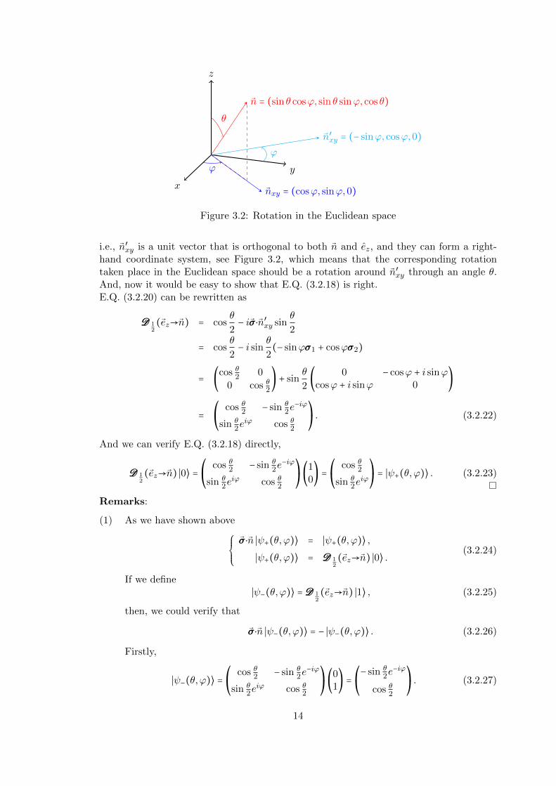
Figure 3.2: Rotation in the Euclidean space
i.e., n′xy is a unit vector that is orthogonal to both n and ez, and they can form a right-hand coordinate system, see Figure 3.2, which means that the corresponding rotationtaken place in the Euclidean space should be a rotation around n′xy through an angle θ.And, now it would be easy to show that E.Q. (3.2.18) is right.E.Q. (3.2.20) can be rewritten as
DDD 12(ez→n) = cos
θ
2− iσσσ⋅n′xy sin
θ
2
= cosθ
2− i sin θ
2(− sinϕσσσ1 + cosϕσσσ2)
= (cos θ2 0
0 cos θ2) + sin
θ
2( 0 − cosϕ + i sinϕ
cosϕ + i sinϕ 0)
=⎛⎝
cos θ2 − sin θ2e
−iϕ
sin θ2eiϕ cos θ2
⎞⎠. (3.2.22)
And we can verify E.Q. (3.2.18) directly,
DDD 12(ez→n) ∣0⟩ =
⎛⎝
cos θ2 − sin θ2e
−iϕ
sin θ2eiϕ cos θ2
⎞⎠(1
0) =
⎛⎝
cos θ2
sin θ2eiϕ
⎞⎠= ∣ψ+(θ,ϕ)⟩ . (3.2.23)
Remarks:
(1) As we have shown above
⎧⎪⎪⎨⎪⎪⎩
σσσ⋅n ∣ψ+(θ,ϕ)⟩ = ∣ψ+(θ,ϕ)⟩ ,∣ψ+(θ,ϕ)⟩ = DDD 1
2(ez→n) ∣0⟩ .
(3.2.24)
If we define∣ψ−(θ,ϕ)⟩ =DDD 1
2(ez→n) ∣1⟩ , (3.2.25)
then, we could verify that
σσσ⋅n ∣ψ−(θ,ϕ)⟩ = − ∣ψ−(θ,ϕ)⟩ . (3.2.26)
Firstly,
∣ψ−(θ,ϕ)⟩ =⎛⎝
cos θ2 − sin θ2e
−iϕ
sin θ2eiϕ cos θ2
⎞⎠(0
1) =
⎛⎝− sin θ
2e−iϕ
cos θ2
⎞⎠. (3.2.27)
14
Then,
σσσ⋅n ∣ψ−(θ,ϕ)⟩ = ( cos θ sin θe−iϕ
sin θeiϕ − cos θ)⎛⎝− sin θ
2e−iϕ
cos θ2
⎞⎠
=⎛⎝− sin θ
2e−iϕ cos θ + cos θ2 sin θe−iϕ
− sin θ2e
−iϕ sin θeiϕ − cos θ2 cos θ
⎞⎠
=⎛⎝
sin θ2e
−iϕ
− cos θ2
⎞⎠
= − ∣ψ−(θ,ϕ)⟩ . (3.2.28)
(2) The spinor representation of the SO(3) group, D(R), satisfies
D(R)x ⋅ σσσD†(R) = x′ ⋅ σσσ, (3.2.29)
in which the vector x is rotated under x′ = Rx, i.e., x′j = Rijxj .Example: D(R) ≡DDD 1
2(ez→n) gives
D(R)σ3D†(R) = σσσ ⋅ n. (3.2.30)
It implies that
σσσ ⋅ n∣n⟩ = D(R)σ3D†(R)D(R)∣ez⟩
= D(R)σ3∣0⟩= ∣n⟩. (3.2.31)
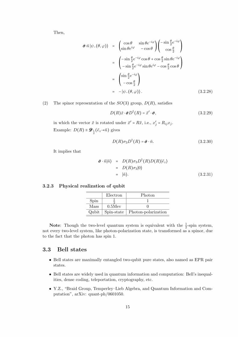
3.2.3 Physical realization of qubit
Electron Photon
Spin 12 1
Mass 0.5Mev 0
Qubit Spin-state Photon-polarization
Note: Though the two-level quantum system is equivalent with the 12 -spin system,
not every two-level system, like photon-polarization state, is transformed as a spinor, dueto the fact that the photon has spin 1.
3.3 Bell states
• Bell states are maximally entangled two-qubit pure states, also named as EPR pairstates.
• Bell states are widely used in quantum information and computation: Bell’s inequal-ities, dense coding, teleportation, cryptography, etc.
• Y.Z., “Braid Group, Temperley–Lieb Algebra, and Quantum Information and Com-putation”, arXiv: quant-ph/0601050.
15

• Y.Z., Jinglong Pang, “Space-Time Topology in Teleportation-Based Quantum Com-putation”, arXiv:1309.0955.
• Y.Z., Kun Zhang, “Bell Transform, Teleportation Operator and Teleportation-BasedQuantum Computation”, arXiv:1401.7009.
3.3.1 Notation
Pauli matrices are unitary matrices defined in spin-12 space:
⎧⎪⎪⎪⎪⎪⎪⎪⎪⎪⎪⎪⎪⎪⎨⎪⎪⎪⎪⎪⎪⎪⎪⎪⎪⎪⎪⎪⎩
σσσx ∶= XXX ∶= (0 11 0
) ;
σσσy ∶= −iYYY ∶= (0 −ii 0
) ;
σσσz ∶= ZZZ ∶= (1 00 −1
) .
(3.3.1)
There we get three quantum gates: quantum gate XXX, quantum gate ZZZ and quantum gateYYY = ZXZXZX.
Def 3.3.1 (Bell states). The following four double-qubit states
⎧⎪⎪⎪⎪⎪⎪⎪⎪⎪⎪⎪⎪⎪⎪⎨⎪⎪⎪⎪⎪⎪⎪⎪⎪⎪⎪⎪⎪⎪⎩
∣φ+⟩ ∶= ∣ψ(0,0)⟩ ∶= 1√2( ∣00⟩ + ∣11⟩ ),
∣φ−⟩ ∶= ∣ψ(0,1)⟩ ∶= 1√2( ∣00⟩ − ∣11⟩ ),
∣ψ+⟩ ∶= ∣ψ(1,0)⟩ ∶= 1√2( ∣01⟩ + ∣10⟩ ),
∣ψ−⟩ ∶= ∣ψ(1,1)⟩ ∶= 1√2( ∣01⟩ − ∣10⟩ ),
(3.3.2)
are the so called Bell states.
Lemma 3.3.1.1. All the four Bell states defined in E.Q. (3.3.2) can be expressed as
∣ψ(i, j)⟩ = (III2⊗XXXiZZZj) ∣ψ(0,0)⟩ , with i, j = 0,1. (3.3.3)
Proof. With the definition of the Bell states (3.3.2), we can check E.Q. (3.3.3) one by onefor all the four cases of i, j = 0,1.
(1) For the case of i = j = 0, E.Q (3.3.3) is absolutely right.
(2) For the case of i = 0, j = 1, the right-hand-side (RHS) of E.Q. (3.3.3) should be
RHS = (III2⊗ZZZ) ∣ψ(0,0)⟩
= (III2⊗ZZZ) 1√2(∣00⟩ + ∣11⟩)
= 1√2(∣00⟩ − ∣11⟩)
= ∣ψ(0,1)⟩ , (3.3.4)
which means E.Q (3.3.3) is correct in this case.
16

(3) For the case of i = 1, j = 0, we evaluate the right-hand-side (RHS) of E.Q. (3.3.3)
RHS = (III2⊗XXX) ∣ψ(0,0)⟩
= (III2⊗XXX) 1√2(∣00⟩ + ∣11⟩)
= 1√2(∣01⟩ + ∣10⟩)
= ∣ψ(1,0)⟩ , (3.3.5)
which also shows the legitimation of E.Q (3.3.3) in this circumstance.
(4) For the case of i = j = 1, we can get the right-hand-side (RHS) of E.Q. (3.3.3)
RHS = (III2⊗XXXZZZ) ∣ψ(0,0)⟩
= (III2⊗XXXZZZ) 1√2(∣00⟩ + ∣11⟩)
= (III2⊗XXX) 1√2(∣00⟩ − ∣11⟩)
= 1√2(∣01⟩ − ∣10⟩)
= ∣ψ(1,1)⟩ , (3.3.6)
which says E.Q (3.3.3) for the last situation.
Now, we can conclude that for all the four cases i, j = 0,1, E.Q (3.3.3) is valid.Remark: For four Bell states (3.3.2), we have the following geometric representations,
∣ψ(00)⟩ = ∣φ+⟩ = 1√2(∣00⟩ + ∣11⟩) = (3.3.7)
∣ψ(10)⟩ = ∣ψ+⟩ = (I2 ⊗XI2 ⊗XI2 ⊗X)∣ψ(00)⟩ = 1√2(∣01⟩ + ∣10⟩) = rXXX (3.3.8)
∣ψ(01)⟩ = ∣φ−⟩ = (I2 ⊗ZI2 ⊗ZI2 ⊗Z)∣ψ(00)⟩ = 1√2(∣00⟩ − ∣11⟩) = rZZZ (3.3.9)
∣ψ(11)⟩ = ∣ψ−⟩ = (I2 ⊗XZI2 ⊗XZI2 ⊗XZ)∣ψ(00)⟩ = 1√2(∣01⟩ − ∣10⟩) = rXZXZXZ (3.3.10)
The vertical line denotes one Hilbert space H2.
Lemma 3.3.1.2. The four Bell states can also be expressed as
∣ψ(i, j)⟩ = 1√2( ∣0i⟩ + (−1)j ∣1i⟩ ), (3.3.11)
where i = (i + 1) mod 2 and i = 0,1.
We can show in the following that E.Q. (3.3.11) is consistent with E.Q. (3.3.2).
17

Proof. From E.Q. (3.3.3) we can get
∣ψ(i, j)⟩ = 1√2(III2⊗XXXiZZZj)( ∣00⟩ + ∣11⟩ )
= 1√2( ∣0⟩⊗XXXiZZZj ∣0⟩ + ∣1⟩⊗XXXiZZZj ∣1⟩ )
= 1√2( ∣0⟩⊗XXXi ∣0⟩ + (−1)j ∣1⟩⊗XXXi ∣1⟩ )
= 1√2( ∣0⟩⊗ ∣i⟩ + (−1)j ∣1⟩⊗ ∣i⟩ ),
which is what exactly E.Q. (3.3.11) shows.
Remark: All the four Bell states defined in E.Q. (3.3.2) are normalized:
(i) ⟨ψ(0,0) ∣ψ(0,0)⟩ = 1, since
1√2( ⟨00∣ + ⟨11∣ ) 1√
2( ∣00⟩ + ∣11⟩ ) = 1
2(⟨00 ∣00⟩ + ⟨00 ∣11⟩ + ⟨11 ∣00⟩ + ⟨11 ∣11⟩)
= 1
2(1 + 0 + 0 + 1)
= 1.
(ii) ⟨ψ(i, j) ∣ψ(i, j)⟩ = 1, because
⟨ψ(i, j) ∣ψ(i, j)⟩ = ( ⟨ψ(0,0)∣III2⊗ZZZjXXXi)(III2⊗XXXiZZZj ∣ψ(0,0)⟩ )
= ⟨ψ(0,0) ∣III2⊗ZZZjXXXiXXXiZZZj ∣ψ(0,0)⟩= ⟨ψ(0,0) ∣ψ(0,0)⟩= 1.
Lemma 3.3.1.3. Let’s MMM denotes an arbitrary SU(2) matrix, namely single-qubit gate,and MMMT is the transpose of MMM . Then
(III2⊗MMM) ∣ψ(0,0)⟩ = (MMMT⊗III2) ∣ψ(0,0)⟩ , (3.3.12)
with the diagrammatical representation
rMMM = rMMMT (3.3.13)
18

Proof. Firstly, evaluate the left-hand-side (LHSLHSLHS) of E.Q. (3.3.12)
LHSLHSLHS = (III2⊗MMM) ∣ψ(0,0)⟩
= III2⊗MMM√2
1
∑i=0
∣ii⟩
= 1√2
1
∑i=0
∣i⟩⊗MMM ∣i⟩
= 1√2( ∣0⟩⊗(M00 ∣0⟩ +M10 ∣1⟩ ) + ∣1⟩⊗(M01 ∣0⟩ +M11 ∣1⟩ ))
= 1√2((M00 ∣0⟩ +M01 ∣1⟩ )⊗ ∣0⟩ + (M10 ∣0⟩ +M11 ∣1⟩ )⊗ ∣1⟩ )
= 1√2(MMMT ∣0⟩⊗ ∣0⟩ +MMMT ∣1⟩⊗ ∣1⟩ )
= MMMT⊗III2√2
( ∣0⟩⊗ ∣0⟩ + ∣1⟩⊗ ∣1⟩ ),
i.e.,
LHSLHSLHS = (MMMT⊗III2) ∣ψ(00)⟩ , (3.3.14)
which happens to be equal to the right-hand-side of E.Q. (3.3.12). In the derivation wehave assumed that MMM has the matrix form
MMM ∶= (M00 M01
M10 M11) ,
namely
MMMT = (M00 M10
M01 M11) .
We may notice that⎧⎪⎪⎪⎨⎪⎪⎪⎩
XXXT = XXX,
ZZZT = ZZZ,
(XZXZXZ)T = ZXZXZX.
(3.3.15)
Therefore, we can get the conclusion that
⎧⎪⎪⎪⎪⎪⎪⎨⎪⎪⎪⎪⎪⎪⎩
∣ψ+⟩ = (III2⊗XXX) ∣ψ(00)⟩ = (XXX⊗III2) ∣ψ(00)⟩ ,
∣φ−⟩ = (III2⊗ZZZ) ∣ψ(00)⟩ = (ZZZ⊗III2) ∣ψ(00)⟩ ,
∣ψ−⟩ = (III2⊗XZXZXZ) ∣ψ(00)⟩ = (ZXZXZX⊗III2) ∣ψ(00)⟩ .
(3.3.16)
∣ψ(10)⟩ = ∣ψ+⟩ = rXXX = rXXX (3.3.17)
∣ψ(01)⟩ = ∣φ−⟩ = rZZZ = rZZZ (3.3.18)
∣ψ(11)⟩ = ∣ψ−⟩ = rXZXZXZ = rZXZXZX (3.3.19)
19

3.3.2 Parity-bit (i) and Phase-bit (j)
• Parity-bit (i)
– i = 0, two spins are aligned, denoted by “φ”;
– i = 1, two spins are anti-aligned, denoted by “ψ”.
• Phase-bit (j)
– j = 0, superposition with “+”, i.e., with equal phase;
– j = 1, superposition with “−”, i.e., with opposite phase.
Table 3.1: Parity-bit (i) and Phase-bit (j)
PPPPPPPPPij
0 1
0 ∣φ+⟩ ∣φ−⟩
1 ∣ψ+⟩ ∣ψ−⟩
Lemma 3.3.2.1. Bell states are eigenstates of the two commutative operators:
1. parity-bit operator: ZZZ⊗ZZZ,
2. phase-bit operator: XXX⊗XXX,
namely⎧⎪⎪⎪⎨⎪⎪⎪⎩
(ZZZ⊗ZZZ) ∣ψ(i, j)⟩ = (−1)i ∣ψ(i, j)⟩ ,
(XXX⊗XXX) ∣ψ(i, j)⟩ = (−1)j ∣ψ(i, j)⟩ .(3.3.20)
Proof. The parity-bit operator and the phase-bit operator are commutative, because
(XXX⊗XXX) (ZZZ⊗ZZZ)= (XZXZXZ)⊗ (XZXZXZ)= (−ZXZXZX)⊗ (−ZXZXZX)= (ZXZXZX)⊗ (ZXZXZX)= (ZZZ⊗ZZZ) (XXX⊗XXX) , (3.3.21)
namely[XXX⊗XXX,ZZZ⊗ZZZ] = 0. (3.3.22)
We may examine the two operators separately.
20

(a) Parity-bit operator ZZZ⊗ZZZ.
(ZZZ⊗ZZZ) ∣ψ(i, j)⟩
= (ZZZ⊗ZZZ) 1√2[ ∣0i⟩ + (−1)j ∣1i⟩ ]
= 1√2[ZZZ ∣0⟩⊗ZZZ ∣i⟩ + (−1)jZZZ ∣1⟩⊗ZZZ ∣i⟩ ]
= 1√2[ ∣0⟩⊗(−1)i ∣i⟩ + (−1)j(−1) ∣1⟩⊗(−1)i−1 ∣i⟩ ]
= 1√2[(−1)i ∣0⟩⊗ ∣i⟩ + (−1)j(−1)i ∣1⟩⊗ ∣i⟩ ]
= (−1)i 1√2[ ∣0⟩⊗ ∣i⟩ + (−1)j ∣1⟩⊗ ∣i⟩ ],
i.e.,
(ZZZ⊗ZZZ) ∣ψ(i, j)⟩ = (−1)i ∣ψ(i, j)⟩ . (3.3.23)
In the derivation, we have used the facts that
⎧⎪⎪⎨⎪⎪⎩
ZZZ ∣i⟩ = (−1)i ∣i⟩ ,ZZZ ∣i⟩ = (−1)i−1 ∣i⟩ .
(3.3.24)
(b) Phase-bit operator XXX⊗XXX.
(XXX⊗XXX) ∣ψ(i, j)⟩
= (XXX⊗XXX) 1√2( ∣0i⟩ + (−1)j ∣1i⟩ )
= 1√2(XXX ∣0⟩⊗XXX ∣i⟩ + (−1)jXXX ∣1⟩⊗XXX ∣i⟩ )
= 1√2( ∣1⟩⊗ ∣i⟩ + (−1)j ∣0⟩⊗ ∣i⟩ )
= (−1)j 1√2( ∣0⟩⊗ ∣i⟩ + (−1)j ∣1⟩⊗ ∣i⟩ ),
namely
(XXX⊗XXX) ∣ψ(i, j)⟩ = (−1)j ∣ψ(i, j)⟩ . (3.3.25)
And we have used the facts in the following to go through the above derivation,
XXX ∣i⟩ = ∣i⟩ ,XXX ∣i⟩ = ∣i⟩ . (3.3.26)
With E.Q. (3.3.23) and E.Q. (3.3.25), we get E.Q. (3.3.20) proved.
3.3.3 Orthonormal basis of the two-qubit Hilbert space
Thm 3.3.3.1. Bell states form an orhonormal basis of two-qubit Hilber space, namely
∣φ+⟩ , ∣ψ+⟩ , ∣φ−⟩ , ∣ψ−⟩
is an orthonormal basis of two-qubit Hilbert space.
21

Proof. Firstly, we would prove that all the Bell states are mutually orthogonal and nor-malized. Secondly, the completeness of the set of the four Bell state vectors would beverified.
(a) The set of the four Bell state vectors make an orthonormal vector set. From E.Q.(3.3.3), we can derive that
⟨ψ(i, j) ∣ψ(i′, j′)⟩ = ⟨ψ(0,0)∣ (III2⊗ZZZjXXXi)(III2⊗XXXi′ZZZj′
) ∣ψ(0,0)⟩
= 1
2( ⟨00∣ + ⟨11∣ )(III2⊗ZZZjXXXi+i′ZZZj
′
)( ∣00⟩ + ∣11⟩ )
= 1
2
1
∑k,`=0
⟨kk∣ (III2⊗ZZZjXXXi+i′Zj′
) ∣``⟩
= 1
2
1
∑k,`=0
⟨k ∣ `⟩⊗ ⟨k∣ZZZjXXXi+i′ZZZj′
∣`⟩
= 1
2
1
∑k,`=0
δk` ⟨k∣ZZZjXXXi+i′ZZZj′
∣`⟩
= 1
2
1
∑k=0
⟨k∣ZZZjXXXi+i′Zj′
∣k⟩
= 1
2tr(ZZZjXXXi+i′ZZZj
′
)
= 1
2tr(ZZZj
′+jXXXi+i′).
BecauseZZZ2 =XXX2 = III2, trZZZ = trXXX = tr (ZXZXZX) = 0,
and i, j, i′, j′∈0,1, then we can obtain
⟨ψ(i, j) ∣ψ(i′, j′)⟩ = δjj′δii′ , (3.3.27)
which means that the four Bell states are mutually orthogonal and are all of unitlength.
In diagrammatical representation, we use the cup configuration for ket state, andcap configuration for bra state, shown as
∣ψ(i′j′)⟩ = rXi′Zj′Xi′Zj′Xi′Zj′ ⟨ψ(ij)∣ = rZjXiZjXiZjXi (3.3.28)
Therefore, the orhonormal relation has the diagrammatical representation
⟨ψ(ij)∣ψ(i′j′)⟩ = rXi′Zj′Xi′Zj′Xi′Zj′
rZjXiZjXiZjXi
(3.3.29)
From the diagrammatical rules, we would have the normalized trace of the single-qubit gates on the loop,
⟨ψ(ij)∣ψ(i′j′)⟩ = 1
2tr(ZZZjXXXiXXXi′ZZZj
′
)
= 1
2tr(ZZZj
′+jXXXi+i′)
= δjj′δii′ . (3.3.30)
22

(b) The vector set consisted of the four Bell states is complete. By utilizing E.Q. (3.3.11),we can get
1
∑i,j=0
∣ψ(i, j)⟩ ⟨ψ(i, j)∣
=1
∑i,j=0
1√2( ∣0i⟩ + (−1)j ∣1i⟩ )( ⟨0i∣ + (−1)j ⟨1i∣ ) 1√
2
= 1
2
1
∑i,j=0
( ∣0i⟩ ⟨0i∣ + (−1)j ∣1i⟩ ⟨0i∣ + (−1)j ∣0i⟩ ⟨1i∣ + ∣1i⟩ ⟨1i∣ ).
As we see that1
∑i,j=0
(−1)j ∣1i⟩ ⟨0i∣ = 0,1
∑i,j=0
(−1)j ∣0i⟩ ⟨1i∣ = 0, (3.3.31)
therefore
1
∑i,j=0
∣ψ(i, j)⟩ ⟨ψ(i, j)∣ = 1
2
1
∑i,j=0
( ∣0i⟩ ⟨0i∣ + ∣1i⟩ ⟨1i∣ )
=1
∑i=0
( ∣0i⟩ ⟨0i∣ + ∣1i⟩ ⟨1i∣ )
=1
∑i,j=0
∣ji⟩ ⟨ji∣
= III4,
i.e.,1
∑i,j=0
∣ψ(i, j)⟩ ⟨ψ(i, j)∣ = III4. (3.3.32)
Remark:
• ∣ψ(i, j)⟩ ∣ i, j = 0,1 is the Bell basis of H2⊗H2;
• ∣i, j⟩ ∣ i, j = 0,1 is the product basis of H2⊗H2.
3.3.4 How to distinguish (create) ∣ψ(i, j)⟩.
There are two different cases
(i) Alice and Bob are in the same lab, which means that the distance between themis very close. Therefore, they can do the measurement jointly, e.g. XXXA⊗XXXB andZZZA⊗ZZZB.
(ii) Alice and Bob are far away from each other, which leaves them two choices:
• perform local measurement, e.g. XXXA⊗IIIB, ZZZA⊗IIIB, IIIA⊗XXXB, and IIIA⊗ZZZB.
• classical communication (phone call).
But, with only local operation (LO) and classical communication (CC), it is impos-sible to distinguish/create ∣ψi,j⟩. The reason is that local operation changes ∣ψ(i, j)⟩,since ⎧⎪⎪⎨⎪⎪⎩
[XXX⊗III2,ZZZ⊗ZZZ] ≠ 0,
[ZZZ⊗III2,XXX⊗XXX] ≠ 0.(3.3.33)
23

Remark: Quantum entanglement cannot be created by remote pairs by using local op-eration and classical communication.
24

Chapter 4
No-Cloning, Dense Coding,Teleportation and Cryptography
Reference:
[Preskill] Chapter 4: Quantum entanglement.
[Nielsen & Chuang] Chapter 2: Introduction to quantum mechanics.
[Nielsen & Chuang] Chapter 12: quantum information theory.
4.1 No-cloning theorem
Def 4.1.1 (Cloning Machine). The cloning machine is a unitary transformation U , whichsatisfies
U( ∣φ⟩⊗ ∣0⟩ ) = ∣φ⟩⊗ ∣φ⟩ (4.1.1)
for arbitrary state ∣φ⟩. It can be represented in the diagram shown in Figure 4.1.
Target object ∣φ⟩UUU
∣φ⟩
Blank object ∣0⟩ ∣φ⟩
Figure 4.1: Copy machine in quantum mechanics
Thm 4.1.0.1 (No-cloning theorem 1). The cloning machine doesn’t exist (in QuantumMechanics).
Proof. For simplicity, we deal with the two-dimensional Hilbert space. As the definition(4.1.1) shows, we choose the blank object to be ∣0⟩ and the target object to be be ∣0⟩ or∣1⟩, and the copy machine satisfies the following equations:
⎧⎪⎪⎪⎨⎪⎪⎪⎩
U ∣0⟩⊗ ∣0⟩ = ∣0⟩⊗ ∣0⟩ ,
U ∣1⟩⊗ ∣0⟩ = ∣1⟩⊗ ∣1⟩ .(4.1.2)
25

For example, the most popular two-qubit quantum gate in quantum computation is theCNOT gate, which has the property,
⎧⎪⎪⎪⎨⎪⎪⎪⎩
CNOT ∣0⟩⊗ ∣0⟩ = ∣0⟩⊗ ∣0⟩ ,
CNOT ∣1⟩⊗ ∣0⟩ = ∣1⟩⊗ ∣1⟩ .(4.1.3)
For ∀ ∣φ⟩ ∈ H2, which has the form of
∣φ⟩ = a ∣0⟩ + b ∣1⟩ , with ∣a∣2 + ∣b∣2 = 1, (4.1.4)
we obtain
U ∣φ⟩⊗ ∣0⟩ = U(a ∣0⟩ + b ∣1⟩ )⊗ ∣0⟩= aU ∣0⟩⊗ ∣0⟩ + bU ∣1⟩⊗ ∣0⟩= a ∣0⟩⊗ ∣0⟩ + b ∣1⟩⊗ ∣1⟩ ,
i.e.,U ∣φ⟩⊗ ∣0⟩ = a ∣0⟩⊗ ∣0⟩ + b ∣1⟩⊗ ∣1⟩ . (4.1.5)
However, the copy machine (4.1.1) tells us another thing:
U ∣φ⟩⊗ ∣0⟩ = ∣φ⟩⊗ ∣φ⟩= (a ∣0⟩ + b ∣1⟩ )⊗(a ∣0⟩ + b ∣1⟩ )= a2 ∣0⟩⊗ ∣0⟩ + b2 ∣1⟩⊗ ∣1⟩ + ab ∣0⟩⊗ ∣1⟩ + ab ∣1⟩⊗ ∣0⟩ . (4.1.6)
In general, E.Q. (4.1.5) and E.Q. (4.1.6) are not consistent with one another. Therefore,the cloning machine is not available for ∀ ∣φ⟩ ∈ H2.
Remarks:
• The copy machine is a non-linear process, but Quantum Mechanics respects linearsuper-position principle.
• The no-cloning theorem is compatible with the Heisenberg uncertainty relation. Ifa state can be exactly copied, then it can be exactly measured, which violates theHeisenberg uncertainty relation.
Thm 4.1.0.2 (No-cloning theorem 2). There is no unitary transformation (cloning ma-chine) which can make copies on distinct non-orthogonal states.
Proof. We firstly consider that case that if such a unitary transformation U exists, whatwe can obtain. And choose two unital state vectors ∣φ⟩ and ∣ψ⟩: being distinct means that
⟨φ ∣ψ⟩ ≠ 1. (4.1.7)
While, being non-orthogonal means that
⟨φ ∣ψ⟩ ≠ 0. (4.1.8)
Because the copy machine U satisfies E.Q. (4.1.1), we find out
(⟨φ∣ ⟨0∣) (∣ψ⟩ ∣0⟩) = ⟨φ∣ ⟨0∣U †U ∣ψ⟩ ∣0⟩= (⟨φ∣ ⟨φ∣) (∣ψ⟩ ∣ψ⟩)= ⟨φ ∣ψ⟩2 ,
26
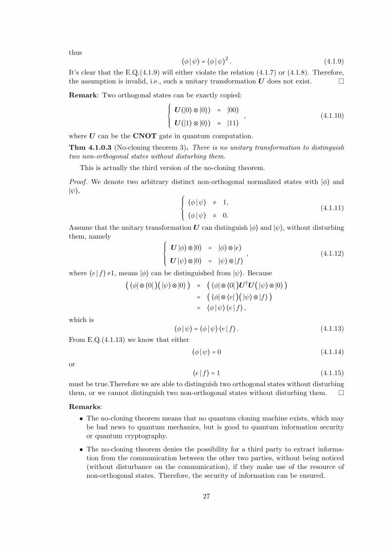
thus⟨φ ∣ψ⟩ = ⟨φ ∣ψ⟩2 . (4.1.9)
It’s clear that the E.Q.(4.1.9) will either violate the relation (4.1.7) or (4.1.8). Therefore,the assumption is invalid, i.e., such a unitary transformation U does not exist.
Remark: Two orthogonal states can be exactly copied:
⎧⎪⎪⎪⎨⎪⎪⎪⎩
U(∣0⟩⊗ ∣0⟩) = ∣00⟩
U(∣1⟩⊗ ∣0⟩) = ∣11⟩, (4.1.10)
where U can be the CNOT gate in quantum computation.
Thm 4.1.0.3 (No-cloning theorem 3). There is no unitary transformation to distinguishtwo non-orthogonal states without disturbing them.
This is actually the third version of the no-cloning theorem.
Proof. We denote two arbitrary distinct non-orthogonal normalized states with ∣φ⟩ and∣ψ⟩,
⎧⎪⎪⎪⎨⎪⎪⎪⎩
⟨φ ∣ψ⟩ ≠ 1,
⟨φ ∣ψ⟩ ≠ 0.(4.1.11)
Assume that the unitary transformation U can distinguish ∣φ⟩ and ∣ψ⟩, without disturbingthem, namely
⎧⎪⎪⎪⎨⎪⎪⎪⎩
U ∣φ⟩⊗ ∣0⟩ = ∣φ⟩⊗ ∣e⟩
U ∣ψ⟩⊗ ∣0⟩ = ∣ψ⟩⊗ ∣f⟩, (4.1.12)
where ⟨e ∣ f⟩≠1, means ∣φ⟩ can be distinguished from ∣ψ⟩. Because
( ⟨φ∣⊗ ⟨0∣ )( ∣ψ⟩⊗ ∣0⟩ ) = ( ⟨φ∣⊗ ⟨0∣ )U †U( ∣ψ⟩⊗ ∣0⟩ )= ( ⟨φ∣⊗ ⟨e∣ )( ∣ψ⟩⊗ ∣f⟩ )= ⟨φ ∣ψ⟩ ⟨e ∣ f⟩ ,
which is⟨φ ∣ψ⟩ = ⟨φ ∣ψ⟩ ⟨e ∣ f⟩ . (4.1.13)
From E.Q.(4.1.13) we know that either
⟨φ ∣ψ⟩ = 0 (4.1.14)
or⟨e ∣ f⟩ = 1 (4.1.15)
must be true.Therefore we are able to distinguish two orthogonal states without disturbingthem, or we cannot distinguish two non-orthogonal states without disturbing them.
Remarks:
• The no-cloning theorem means that no quantum cloning machine exists, which maybe bad news to quantum mechanics, but is good to quantum information securityor quantum cryptography.
• The no-cloning theorem denies the possibility for a third party to extract informa-tion from the communication between the other two parties, without being noticed(without disturbance on the communication), if they make use of the resource ofnon-orthogonal states. Therefore, the security of information can be ensured.
27

4.2 Dense coding
∣φ+⟩(1st qubit) Alice Bob (2nd qubit)
Alice sends a qubit
Bob gets two-bits of information
Dense coding is that, with the entangled resource, Alice sends Bob two classical bitsof information by transmitting a qubit to Bob1. Dense coding can be executed in thefollowing manner step by step:
Step 1: Experiment setup.Alice and Bob share a maximally entangled state, e.g.
Alice Bob∣φ+⟩AB
which is the cup representation for the Bell state ∣φ+⟩ defined in (3.3.7).
Step 2: Local unitary transformation.Alice chooses one of the four unitary transformation I2,X,Z,ZX and per-forms it on her qubit.
∣ψ(0,0)⟩ = 1√2( ∣00⟩ + ∣11⟩ ) (4.2.1)
Alice Bob
I2I2I2∣ψ(00)⟩AB =
Alice Bob
I2I2I2=
∣ψ(0,1)⟩ = 1√2( ∣00⟩ − ∣11⟩ )
= I2⊗Z ∣ψ(0,0)⟩ Bob
= Z⊗I2 ∣ψ(0,0)⟩ Alice (4.2.2)
Alice Bob
ZZZ∣ψ(01)⟩AB =
Alice Bob
ZZZ=
∣ψ(1,0)⟩ = 1√2( ∣01⟩ + ∣10⟩ )
= I2⊗X ∣ψ(0,0)⟩ Bob
= X⊗I2 ∣ψ(0,0)⟩ Alice (4.2.3)
1Note: The Holevo bound (Old Chapter 5.4.1, page 36, John Preskill’s lecture notes) says that withoutentanglement at most a classical bit information can be transmitted via sending a qubit.
28

Alice Bob
XXX∣ψ(10)⟩AB =
Alice Bob
XXX=
∣ψ(1,1)⟩ = 1√2( ∣01⟩ − ∣10⟩ )
= I2⊗XZ ∣ψ(0,0)⟩ Bob
= ZX⊗I2 ∣ψ(0,0)⟩ Alice (4.2.4)
Alice Bob
ZXZXZX∣ψ(11)⟩AB =
Alice Bob
XZXZXZ=
The texts “Bob” and “Alice” appearing in the above equations mean that thecorresponding systems, that are “Bob” and “Alice”, on which the associatednontrivial local unitary transformations are to be performed to obtain the rightfultarget states.
Step 3: Qubit transmission.Alice sends her qubit to Bob.
Alice Bob
XiZjXiZjXiZj
Bob
XiZjXiZjXiZj
Step 4: Bell measurements.Bob performs the Bell measurement:
(X⊗X) ∣ψ(ij)⟩ = (−1)j ∣ψ(ij)⟩ , (4.2.5)
which gives the parity bit i, and
(Z⊗Z) ∣ψ(ij)⟩ = (−1)i ∣ψ(ij)⟩ (4.2.6)
from which gives the phase bit j. With (i, j), Bob get two bits of information.
As we see that, for each two-bit (i, j) that Alice wants to send to Bob, she just modifiesthe qubit in her system with the corresponding local unitary transformation by utilizingthe protocol as illustrated in Table 4.1, and then transmits such the qubit to Bob.Remarks:
• On the one hand, the word “dense” in dense coding means that sending one qubitis to transmit two classical bits.
• On the other hand, we still have that sending two qubits is to transmit two classicalbits, if we think about it the following way: Alice prepares the entangled state ∣φ+⟩and then sends one qubit to Bob, so Alice sends two qubits to Bob in the entireprocedure.
29

Table 4.1: Dense coding
Local unitary transf. Final state Two bits
Alice Bob Bob
I2 ∣φ+⟩ = ∣ψ(0,0)⟩ (0,0)
X ∣ψ+⟩ = ∣ψ(1,0)⟩ (1,0)
Z ∣φ−⟩ = ∣ψ(0,1)⟩ (0,1)
ZX ∣ψ−⟩ = ∣ψ(1,1)⟩ (1,1)
4.3 Quantum teleportation
• Y.Z., “Braid Group, Temperley–Lieb Algebra, and Quantum Information and Com-putation”, arXiv: quant-ph/0601050.
• Y.Z., Jinglong Pang, “Space-Time Topology in Teleportation-Based Quantum Com-putation”, arXiv:1309.0955.
• Y.Z., Kun Zhang, “Bell Transform, Teleportation Operator and Teleportation-BasedQuantum Computation”, arXiv:1401.7009.
In some sense, Quantum Teleportation is a kind of inverse process of dense coding (seeTable 4.2).
∣φ+⟩(1st qubit) Alice Bob (2nd qubit)
Alice sends two classical bits to Bob
Bob gets one qubit from Alice
Table 4.2: Dense coding vs. Quantum teleportation
Resource Send transmit
Dense coding∣φ+⟩
1 qubit 2 bits
Quantum Teleportation 2 bits 1 qubit
Task: Alice wants to send an unknown qubit to Bob, who is far away from her.
Lemma 4.3.0.1.
∣ψ⟩⊗ ∣φ+⟩ = 1
2( ∣φ+⟩⊗ ∣ψ⟩ + (X⊗I2 ∣φ+⟩ )⊗X ∣ψ⟩ + (Z⊗I2 ∣φ+⟩ )⊗Z ∣ψ⟩
+ (ZX⊗I2 ∣φ+⟩ )⊗XZ ∣ψ⟩,) (4.3.1)
30

which can be represented in the diagram formulism also,
∣ψ⟩ ∣φ+⟩
= 12
⎧⎪⎪⎨⎪⎪⎩+ XXX XXX + ZZZ ZZZ + ZXZXZX XZXZXZ
⎫⎪⎪⎬⎪⎪⎭.
(4.3.2)
Proof. We can give an expression to unknown state ∣ψ⟩
∣ψ⟩ ∶=a ∣0⟩ + b ∣1⟩ , with a, b ∈ C and a2 + b2 = 1. (4.3.3)
From the definition of the four Bell states (3.3.2), we can get
⎧⎪⎪⎪⎪⎪⎪⎪⎪⎪⎪⎪⎪⎪⎨⎪⎪⎪⎪⎪⎪⎪⎪⎪⎪⎪⎪⎪⎩
∣00⟩ = 1√2( ∣φ+⟩ + ∣φ−⟩ ),
∣01⟩ = 1√2( ∣ψ+⟩ + ∣ψ−⟩ ),
∣10⟩ = 1√2( ∣ψ+⟩ − ∣ψ−⟩ ),
∣11⟩ = 1√2( ∣φ+⟩ − ∣φ−⟩ ).
(4.3.4)
With these materials we can make the following derivation
∣ψ⟩ ∣φ+⟩
= 1√2(a ∣0⟩ + b ∣1⟩ )( ∣00⟩ + ∣11⟩ )
= 1√2[a ∣0⟩ ( ∣00⟩ + ∣11⟩ ) + b ∣1⟩ ( ∣00⟩ + ∣11⟩ )]
= 1√2[a( ∣00
¯0⟩ + ∣01
¯1⟩ ) + b( ∣10
¯0⟩ + ∣11
¯1⟩ )]
= 1
2[a( ∣φ+⟩ + ∣φ−⟩ ) ∣0⟩ + b( ∣ψ+⟩ − ∣ψ−⟩ ) ∣0⟩
+ a( ∣ψ+⟩ + ∣ψ−⟩ ) ∣1⟩ + b( ∣φ+⟩ − ∣φ−⟩ ) ∣1⟩ ]
= 1
2[∣φ+⟩(a ∣0⟩ + b ∣1⟩ ) + ∣φ−⟩(a ∣0⟩ − b ∣1⟩ )
+ ∣ψ+⟩(a ∣1⟩ + b ∣0⟩ ) + ∣ψ−⟩(a ∣1⟩ − b ∣0⟩ )]
= 1
2[∣φ+⟩⊗∣ψ⟩ + (Z⊗I2∣φ+⟩)⊗(Z ∣ψ⟩ ) + (X⊗I2) ∣φ+⟩⊗(X ∣ψ⟩ )
+ (ZX⊗III2 ∣φ+⟩ )(XZ ∣ψ⟩ )],
which is equivalent to E.Q. (4.3.1). Therefore, Lemma 4.3.0.1 has been proved.
Remarks: Magic of QM.
• With the superposition principle in QM, for one state, it can be realized by thesuperposition of many other states, namely Lemma 4.3.0.1. (1→ N)
31

• In QM, wave function collapse due to the measurement process, i.e., measurementcan extract one state from the superposition of many other states. (N → 1)
The Quantum Telecportation can be accomplished with the following steps:
Step 1: State preparation.Alice and Bob share the entangled state ∣φ+⟩. And Alice has the unknown qubit∣ϕ⟩A in hand. This can also be represented in the form of diagram:
∣ϕ⟩A ∣φ+⟩A B.
Alice & Bob:
Step 2: Bell measurement by Alice.Alice makes joint measurement for the observables X⊗X and Z⊗Z, on thecomposite of the subsystem A and the unknown particle that Alice wants tosend to Bob. The measurement results and the two-bit information associatedwith the measurement datum, along with post measurement states, are listed inTable 4.3.
Table 4.3: Alice’s measurement result and the two-bit information
post-measurement state Z⊗Z X⊗X two-bit
∣φ+⟩ 1 1 (0,0)
∣φ−⟩ 1 −1 (0,1)
∣ψ+⟩ −1 1 (1,0)
∣ψ−⟩ −1 −1 (1,1)
It is transparent to that the measurement of the observables X⊗X and Z⊗Zare equivalent to the projection measurements for the Bell measurement, definedas
⎧⎪⎪⎪⎪⎪⎪⎪⎪⎪⎪⎨⎪⎪⎪⎪⎪⎪⎪⎪⎪⎪⎩
E00 ∶= ∣φ+⟩ ⟨φ+∣ ,
E01 ∶= ∣φ−⟩ ⟨φ−∣ ,
E10 ∶= ∣ψ+⟩ ⟨ψ+∣ ,
E11 ∶= ∣ψ−⟩ ⟨ψ−∣ ,
(4.3.5)
which can be represented in a diagrammatic formalism shown as
EEE00 = , EEE01 =XXX
XXX
,
EEE10 =ZZZZZZ
, EEE11 =ZXZXZX
XZXZXZ.
32

We now utilize Lemma 4.3.0.1, which actually means
∣ψ⟩⊗ ∣φ+⟩ = 1
2(∣φ+⟩⊗∣ψ⟩ + ∣φ−⟩⊗(Z ∣ψ⟩ ) + ∣ψ+⟩⊗(X ∣ψ⟩ )
+ ∣ψ−⟩ )(XZ ∣ψ⟩ )). (4.3.6)
Therefore, after the Bell measurement carried out on the qubit of Alice and theunknown state, we obtain
⎧⎪⎪⎪⎪⎪⎪⎪⎪⎪⎪⎪⎪⎪⎨⎪⎪⎪⎪⎪⎪⎪⎪⎪⎪⎪⎪⎪⎩
( ∣φ+⟩ ⟨φ+∣⊗I2)( ∣ψ⟩⊗ ∣φ+⟩ ) = 12 ∣φ+⟩⊗∣ψ⟩,
( ∣φ−⟩ ⟨φ−∣⊗I2)( ∣ψ⟩⊗ ∣φ+⟩ ) = 12 ∣φ−⟩⊗Z ∣ψ⟩,
( ∣ψ+⟩ ⟨ψ+∣⊗I2)( ∣ψ⟩⊗ ∣φ+⟩ ) = 12 ∣ψ+⟩⊗X ∣ψ⟩,
( ∣ψ−⟩ ⟨ψ−∣⊗I2)( ∣ψ⟩⊗ ∣φ+⟩ ) = 12 ∣ψ−⟩⊗XZ ∣ψ⟩.
(4.3.7)
E.Q.(4.3.7) can also be rewritten in the diagram language shown in the followingcontext:
• ( ∣φ+⟩ ⟨φ+∣⊗I2)( ∣ψ⟩⊗ ∣φ+⟩ ) = 12 ∣φ+⟩⊗∣ψ⟩
Measurement
A A B
=Preparation
12
BA A (4.3.8)
• ( ∣φ−⟩ ⟨φ−∣⊗I2)( ∣ψ⟩⊗ ∣φ+⟩ ) = 12 ∣φ−⟩⊗Z ∣ψ⟩
ZZZ
ZZZMeasurement
A A B
=Preparation
12
ZZZZZZ
BA A (4.3.9)
• ( ∣ψ+⟩ ⟨ψ+∣⊗I2)( ∣ψ⟩⊗ ∣φ+⟩ ) = 12 ∣ψ+⟩⊗X ∣ψ⟩
XXX
XXXMeasurement
A A B
=Preparation
12
XXX
XXX
BA A (4.3.10)
• ( ∣ψ−⟩ ⟨ψ−∣⊗I2)( ∣ψ⟩⊗ ∣φ+⟩ ) = 12 ∣ψ−⟩⊗XZ ∣ψ⟩
XZXZXZ
ZXZXZXMeasurement
A A B
=Preparation
12
ZXZXZX
XZXZXZ
BA A (4.3.11)
33
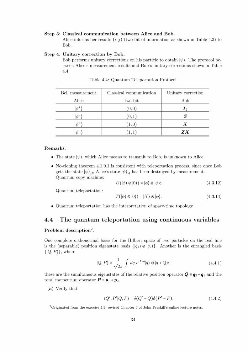
Step 3: Classical communication between Alice and Bob.Alice informs her results (i, j) (two-bit of information as shown in Table 4.3) toBob.
Step 4: Unitary correction by Bob.Bob performs unitary corrections on his particle to obtain ∣ψ⟩. The protocol be-tween Alice’s measurement results and Bob’s unitary corrections shows in Table4.4.
Table 4.4: Quantum Teleportation Protocol
Bell measurement Classical communication Unitary correction
Alice two-bit Bob
∣φ+⟩ (0,0) I2
∣φ−⟩ (0,1) Z
∣ψ+⟩ (1,0) X
∣ψ−⟩ (1,1) ZX
Remarks:
• The state ∣ψ⟩, which Alice means to transmit to Bob, is unknown to Alice.
• No-cloning theorem 4.1.0.1 is consistent with teleportation process, since once Bobgets the state ∣ψ⟩B, Alice’s state ∣ψ⟩A has been destroyed by measurement.Quantum copy machine:
U(∣φ⟩⊗ ∣0⟩) = ∣φ⟩⊗ ∣φ⟩; (4.3.12)
Quantum teleportation:T (∣φ⟩⊗ ∣0⟩) = ∣X⟩⊗ ∣φ⟩. (4.3.13)
• Quantum teleportation has the interpretation of space-time topology.
4.4 The quantum teleportation using continuous variables
Problem description2:
One complete orthonormal basis for the Hilbert space of two particles on the real lineis the (separable) position eigenstate basis ∣q1⟩ ⊗ ∣q2⟩. Another is the entangled basis∣Q,P ⟩, where
∣Q,P ⟩ = 1√2π∫ dq eiP ⋅q ∣q⟩⊗ ∣q +Q⟩; (4.4.1)
these are the simultaneous eigenstates of the relative position operator QQQ ≡ qqq2−qqq1 and thetotal momentum operator PPP ≡ ppp1 + ppp2.
(a) Verify that
⟨Q′, P ′∣Q,P ⟩ = δ(Q′ −Q)δ(P ′ − P ); (4.4.2)
2Originated from the exercise 4.3, revised Chapter 4 of John Preskill’s online lecture notes.
34

(b) Since the states ∣Q,p⟩ are a basis, we can expand a position eigenstate as
∣q1⟩⊗ ∣q2⟩ = ∫ dQdP ∣Q,P ⟩⟨Q,P ∣(∣q1⟩⊗ ∣q2⟩). (4.4.3)
Evaluate the coefficients ⟨Q,P ∣(∣q1⟩⊗ ∣q2⟩).
(c) Alice and Bob have prepared the entangled state of two particles A and B ; Alice haskept particle A ad Bob has particle B ; Now Alice has received an unknown singleparticle wavepacket ∣ψ⟩C = ∫ dq∣q⟩C C⟨q∣ψ⟩C that she intends to teleport to Bob.Design a protocol that they can execute to achieve the teleportation. What shouldAlice measure? What information should she send to Bob? What should Bob dowhen he receives this information, so that particle B will be prepared in the state∣ψ⟩B?
1) Background: Quantum teleportation is a quantum information protocol in whichAlice and Bob are space-like separated, but Alice can send Bob a qubit based on theapplication of both quantum entanglement and quantum measurement. This protocolusually consists of the four steps:
i) State preparation
ii) Bell measurement
iii) Classical communication
iv) Unitary correction
2) Notation:
∣Ω⟩ = ∫ dq∣qq⟩ = ∣Q = 0, P = 0⟩ =(4.4.4)
Define the U(1) phase operator as
UUUP = e−iP ⋅q = ∫ dq′e−iP ⋅q′
∣q′⟩⟨q′∣, (4.4.5)
UUU−P ∣q⟩ = eiP ⋅q ∣q⟩. (4.4.6)
The unitary formalism shows as
UUU †P = UUU−P , ⟨q∣UUU †
P = ⟨q∣UUU−P = ⟨q∣eiP ⋅q. (4.4.7)
Define the translation operator as
TTTQ = e−ip⋅Q = ∫ dq′∣q′ +Q⟩⟨q′∣, (4.4.8)
TTTQ∣q⟩ = ∣q +Q⟩. (4.4.9)
The unitary formalism shows as
TTT †Q = TTT−Q, ⟨q∣TTT †
Q = ⟨q∣TTT−Q = ⟨q +Q∣, (4.4.10)
⟨q∣∫ dq′∣q′ −Q⟩⟨q′∣ = ∫ dq′δq,q′−Q⟨q′∣ = ⟨q +Q∣. (4.4.11)
Note we have the relations
UUUPTTTQ∣q⟩ = UUUP ∣q +Q⟩ = e−iP ⋅(q+Q)∣q +Q⟩, (4.4.12)
35

TTTQUUUP ∣q⟩ = TTTQe−iP ⋅q ∣q⟩ = e−iP ⋅q ∣q +Q⟩, (4.4.13)
thereforeUUUPTTTQ = e−iP ⋅QTTTQUUUP . (4.4.14)
The entangled basis is defined as
∣Q,P ⟩ = (UUU−P ⊗TTTQ)∣Ω⟩ = ∫ dqeiP ⋅q ∣q, q +Q⟩ (4.4.15)
with the cup configuration
∣Q,P ⟩ = −P Q(4.4.16)
And the cap configuration expresses as
⟨Q,P ∣ = P −Q(4.4.17)
The normalization relation in diagrammatical language:
⟨Q′, P ′∣Q,P ⟩ = = δ(P − P ′)δ(Q −Q′).P ′
−P
−Q′
Q(4.4.18)
Other diagrammatical rules:
−P = −P Q = −Q(4.4.19)
−P Q = −P
Q
(4.4.20)
The product state has the diagrammatical representation:
∣q1, q2⟩ =∇∣q1⟩
∇∣q2⟩
The inner product of product state with the entangled state ∣Q,P ⟩ has the expression
⟨Q,P ∣q1, q2⟩ =∇∣q1⟩
∇∣q2⟩
P −Q = 1√2πe−iP ⋅q1δ(Q − (q2 − q1)).
Note that Q stands for the relative position of two particles, namely Q = q2 − q1.
3) Continuous teleportation:
36

i) State preparation
−P Q∇
∣ψ⟩C ∣Q,P ⟩AB (4.4.21)
where ∣ψ⟩C is the unknown state, expressed as
∣ψ⟩C = ∫ dq∣q⟩C⟨q∣ψ⟩C = ∫ dqψ(q)∣q⟩. (4.4.22)
ii) Bell measurement
−P ′ Q′
P ′ −Q′
C A B (4.4.23)
iii) Topological operation
−P ′ Q′
∇
P ′ −Q′
∣ψ⟩C ∣Q,P ⟩AB
−P Q
=
−P ′ Q′
∇
Q
−P
Q′
P ′
∣ψ⟩B
iv) Unitary correction
After Bell measurement, Bob will obtain the state
∣∣∣ψ⟩B = TTTQUUU−PTTTQ′UUUP ′ ∣ψ⟩B. (4.4.24)
Therefore, he is required to perform the unitary correction
UUU † = UUU−P ′TTT−Q′UUUPTTT−Q = e−iP ⋅Q′
UUUP−P ′TTT−Q−Q′ , (4.4.25)
where the commutative relation (4.4.14) has been applied.
4.5 Quantum cryptography (information security)
4.5.1 Classical cryptography
Alice and Bob want to communicate (transmit information) with each other.
1. To ensure information security, they choose to get an encryption key, e.g.
K ∶= (1 1 1 1 1).
2. Now, Alice wants to send Bob some information, e.g.
A ∶= (0 1 0 0 0).
For information security consideration, she would encrypt her information beforesending out, i.e.,
A +K = (1 0 1 1 1).
37
3. Bob then receives the message, namely
B ∶=A +K.
To read the message, Bob will have to decrypt it, i.e.,
B +K = A +K +K = A.
Remark: The encryption key is the most important thing for information security. Inclassical physics, the key can be copied without Alice and Bob’s notice, by a third partydifferent from Alice and Bob, who we can name “Eve”.
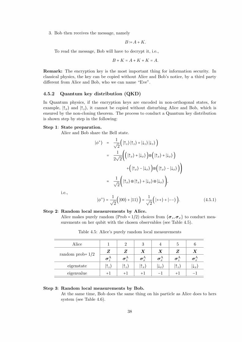
4.5.2 Quantum key distribution (QKD)
In Quantum physics, if the encryption keys are encoded in non-orthogonal states, forexample, ∣↑x⟩ and ∣↑z⟩, it cannot be copied without disturbing Alice and Bob, which isensured by the non-cloning theorem. The process to conduct a Quantum key distributionis shown step by step in the following:
Step 1: State preparation.Alice and Bob share the Bell state.
∣φ+⟩ = 1√2( ∣↑z⟩ ∣↑z⟩ + ∣↓z⟩ ∣↓z⟩ )
= 1
2√
2(( ∣↑x⟩ + ∣↓x⟩ )⊗( ∣↑x⟩ + ∣↓x⟩ )
+( ∣↑x⟩ − ∣↓x⟩ )⊗( ∣↑x⟩ − ∣↓x⟩ ))
= 1√2( ∣↑x⟩⊗ ∣↑x⟩ + ∣↓x⟩⊗ ∣↓x⟩ ),
i.e.,
∣φ+⟩ = 1√2( ∣00⟩ + ∣11⟩ ) = 1√
2( ∣++⟩ + ∣−−⟩ ). (4.5.1)
Step 2: Random local measurements by Alice.Alice makes purely random (Prob = 1/2) choices from σz,σx to conduct mea-surements on her qubit with the chosen observables (see Table 4.5).
Table 4.5: Alice’s purely random local measurements
Alice 1 2 3 4 5 6
random prob= 1/2 Z Z X X Z X
σAz σA
z σAx σA
x σAz σA
x
eigenstate ∣↑z⟩ ∣↑z⟩ ∣↑x⟩ ∣↓x⟩ ∣↑z⟩ ∣↓x⟩eigenvalue +1 +1 +1 −1 +1 −1
Step 3: Random local measurements by Bob.At the same time, Bob does the same thing on his particle as Alice does to herssystem (see Table 4.6).
38
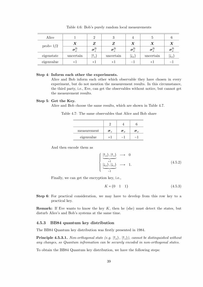
Table 4.6: Bob’s purely random local measurements
Alice 1 2 3 4 5 6
prob= 1/2 X Z Z X X X
σBx σB
z σBz σB
x σBx σB
x
eigenstate uncertain ∣↑z⟩ uncertain ∣↓x⟩ uncertain ∣↓x⟩eigenvalue +1 +1 +1 −1 +1 −1
Step 4: Inform each other the experiments.Alice and Bob inform each other which observable they have chosen in everyexperiment, but do not mention the measurement results. In this circumstance,the third party, i.e., Eve, can get the observables without notice, but cannot getthe measurement results.
Step 5: Get the Key.Alice and Bob choose the same results, which are shown in Table 4.7.
Table 4.7: The same observables that Alice and Bob share
2 4 6
measurement σz σx σx
eigenvalue +1 −1 −1
And then encode them as
⎧⎪⎪⎪⎪⎪⎪⎨⎪⎪⎪⎪⎪⎪⎩
∣↑x⟩ , ∣↑z⟩´¹¹¹¹¹¹¹¹¹¹¹¹¹¸¹¹¹¹¹¹¹¹¹¹¹¹¹¹¶
+1
Ð→ 0
∣↓x⟩ , ∣↓z⟩´¹¹¹¹¹¹¹¹¹¹¹¹¹¸¹¹¹¹¹¹¹¹¹¹¹¹¹¹¶
−1
Ð→ 1.(4.5.2)
Finally, we can get the encryption key, i.e.,
K = (0 1 1) (4.5.3)
Step 6: For practical consideration, we may have to develop from this row key to apractical key.
Remark: If Eve wants to know the key K, then he (she) must detect the states, butdisturb Alice’s and Bob’s systems at the same time.
4.5.3 BB84 quantum key distribution
The BB84 Quantum key distribution was firstly presented in 1984.
Principle 4.5.3.1. Non-orthogonal state (e.g. ∣↑x⟩ , ∣↑z⟩), cannot be distinguished withoutany changes, so Quantum infromation can be securely encoded in non-orthogonal states.
To obtain the BB84 Quantum key distribution, we have the following steps:
39

Step1: Alice randomly prepares one of the four states
∣↑z⟩ , ∣↓z⟩ , ∣↑x⟩ , ∣↓x⟩ ,
and labels∣↑z⟩ , ∣↓z⟩
with its observable Z, while∣↑x⟩ , ∣↓x⟩
with X.
Step2: Alice sends her state to Bob. Bob then makes a random measurement on observ-able X or Z.
Step3: Alice and Bob inform each other their observables, not including measurementoutcomes.
Step4: Alice and Bob keep states in which the same observable are exploited, and keepthe remaining outcomes as the raw key.
∣↑x⟩ , ∣↑z⟩ Ð→ 0∣↓x⟩ , ∣↓z⟩ Ð→ 1
.
Step5: Develop the row key to a practical key.
40

Chapter 5
Bell Inequalities
⋯what is proved by impossibility proofs is lack of imagination.
—John Bell
The true logic of this world is in the calculus of probabilities.
—James Clerk Maxwell
Reference:
[Preskill] Chapter 4: Quantum entanglement;
Lorenzo Maccone, “A simple proof of Bell’s inequality”, arXiv: 1212.5214v2.
5.1 Einstein’s quantum mechanics: local hidden variabletheory (LHV)
5.1.1 What hidden variable (HV) theory?
In Einstein’s opinion, quantum theory is not complete and the reason is that a completetheory should be deterministic. He explained further that quantum randomness is a resultof our ignorance of local hidden variables, and the local hidden variable theory is complete.In other words, quoting the famous statement by Einstein, “God does not play dice.” Wemay show it in the table 5.1. But, Bohr didn’t agree with him, and argued that the
Table 5.1: QM and LHV
Quantum theory Hidden variable theory
∣ψ⟩ = α ∣0⟩ + β ∣1⟩ (∣ψ⟩ , λ), λ: hidden variable
quantum theory is complete, and the measurement output has to be probabilistic, whichis the intrinsic character of quantum mechanics. They were the two greatest minds in the20th century, but held opposite opinions concerning quantum mechanics. Whose opinionis right? It should be answered by the experiment, and there is no other way. Up to now,experiments always agree with Bohr’s viewpoint.
41
5.1.2 What local theory?
As we know that one of the two axioms of Special Relativity is that there is no faster-than-light communication, which ensures the causality. We call this the “relativistic locality”.From that, we can infer that two events at space-like separated regions can not have anycausal connection. Einstein thought that if two subsystems A and B are space-like sepa-rated, measurements on subsystem A cannot modify subsystem B, neither measurementson subsystem B can modify subsystem A. We call this principle as Einstein’s locality.
Einstein’s locality can be violated in quantum mechanics, under a given circumstance.For example, when the two subsystems A and B share the Bell state ∣φ+⟩ (3.3.2), Alicemeasures her subsystem A along the z-axis, and Bob measures his subsystem B soon afterAlice’s measurements, and Bob’s results will be the same as Alice’s results. Afterwards,Alice measures her subsystem A along the x-axis, and Bob measures his subsystem Bsoon after Alice’s measurements, and Bob’s results will be still the same as Alice’s results.Hence, Bob’s measurement results can be modified by Alice’s measurements. With theGHJW theorem 9.4.2.1, we know that if two subsystems A and B share an entangled statein the composite system HA⊗HB, local measurements on subsystem (e.g., B) can leadto different state ensembles for another subsystem (e.g., A), even if the two subsystemsare space-like separated, but, which does not cause the faster-than-light information com-munication. Note that “information is physical”. If there are no classical communicationbetween Alice and Bob, then Alice’s measurements do not modify the ensemble descrip-tion for subsystem B. Therefore, the relativistic causality survives quantum mechanics butEinstein’s locality does not.
5.1.3 The rule to justify the rightful theory
The local hidden variable theory (LHV) contradicts with quantum mechanics, but whichof these two theories is right? Of course, it should be eventually answered by experiments.How can an experiment tell us which one is right, or what kind of experiments can distin-guish these two theories? Bell’s inequality is derived for this purpose, and we can directlycheck the Bell’s inequality in our experiment, from the result we will know which theoryis telling the truth.
5.2 Bell’s inequality in the local hidden variable theory
Let’s consider the following experiment:
(1) Alice has three coins, each with head or tail face. We can label the three coins,which Alice holds, with 1A, 2A and 3A respectively. For each coin we assign aspecific variable to describe the state of the coin, i.e., x for coin 1A, y for coin 2A
and z for coin 3A, and
x, y, z ∈H,T, with “H” for Head, and “T” for Tail.
(2) The local hidden theory allows us to assign the probability distribution of the threecoins faces, denoted as Prob(x, y, z), with x, y, z∈H,T. And we shall know thatthe total probability should be
∑x,y,z∈H,T
Prob(x, y, z) = 1.
42

The probability that the i-th coin and the j-th coin have the same value can bedenoted as Psame(i, j), e.g.
Psame(1,2) ∶=Prob(H,H,H)+Prob(H,H,T)+Prob(T,T,H)+Prob(T,T,T). (5.2.1)
Now,we can define
BI ∶=Psame(1,2) + Psame(1,3) + Psame(2,3), (5.2.2)
and evaluate it in the following way
BI = Prob(H,H,H) +Prob(H,H,T) +Prob(T,T,H) +Prob(T,T,T)+Prob(H,H,H) +Prob(H,T,H) +Prob(T,H,T) +Prob(T,T,T)+Prob(H,H,H) +Prob(T,H,H) +Prob(H,T,T) +Prob(T,T,T)
= 1 + 2(Prob(H,H,H) +Prob(T,T,T)) (5.2.3)
i.e.,BI = Psame(1,2) + Psame(1,3) + Psame(2,3) ≥ 1, (5.2.4)
which is the so-called Bell’s inequality.
In the logical of probabilities distribution, we have the following Venn diagram todescribe Prob(x, y, z), shown in Figure 5.1. For another method of calculation BI,with the help of the diagram, we obtain
BI ∶= Psame(1,2) + Psame(1,3) + Psame(2,3)= (A +C) + (B +C) + (C +D)= 1 + 2C
= 1 + 2(Prob(H,H,H) +Prob(T,T,T))
≥ 1, (5.2.5)
where, through derivation, we have applied the relation A +B + C +D = 1, due toevery time at leats two coins share the same face value.
Note: The Bell’s inequality actually says one simple thing, i.e., for three coinsplaced on the table, there would be at least two coins shown the same face up ordown, in any circumstances.
(3) Mutually Exclusive Experiments (MEE) or Complementary experiment: Each timeAlice is allowed to measure just one coin, namely, the other two coins are forbiddento measure. Then x, y and z are called complementary variables, which means youcannot have two values of them simultaneously.Remark: LHV agrees with MEE.
(4) Perfect correlation.
• Alice and Bob are space-like separated.
• Bob also has three coins, which is numbered with 1B, 2B, and 3B.
• Alice and Bob obtain the same results when measuring their coins with thesame label, i.e., when Alice measures the coin iA and Bob measures the coiniB, with i = 1,2,3, then their results are always coincide.
43

A
CB D
1 2
3
Figure 5.1: Venn diagram of probabilities distribution Prob(x, y, z). The circles labeledby 1, 2 and 3 represent the corresponding probabilities distribution of coin 1, 2 and 3.The overlap regions labeled by A, B, C and D stand for the probability of the coin i andj have the same face value, e.g. region A tells us that coin 1 and 2 share the same facevalue, whereas coin 1 and 3, coin 2 and 3, have the different values.
• This correlation can be proved by classical communications between Alice andBob.
Remark: LHV agrees with the perfection correlation because Alice and Bob arespace-like separated.
(5) With the perfect correlation, for a set of complementary variables, the Bell’s inequal-ities can be checked, and so the local hidden variable theory.
5.3 Bell’s inequality in quantum mechanics
(1) Experiment setup: Alice and Bob share the spin singlet state ∣ψ−⟩,
∣ψ−⟩ = 1√2( ∣01⟩ − ∣10⟩ ). (5.3.1)
Here, we replaced a coin with a spin polarization direction. For example, we canchoose the three orientations ai, i = 1,2,3, for Alice’s system, and bi, i = 1,2,3, forBob’s system, with
∥ai∥ = ∥bi∥ = 1, and ai≠aj , bi≠bj , if i ≠ j.
A spin pointing along the positive (negative) direction of an orientation correspondsto a coin with “Head” (“Tail”) face.
(2) Mutually Exclusive Experiment (MEE).Because ⎧⎪⎪⎨⎪⎪⎩
[σσσ⋅ai, σσσ⋅aj] ≠ 0, if i ≠ j,
[σσσ ⋅bi, σσσ ⋅bj] ≠ 0, if i ≠ j,
which means that σσσ⋅ai and σσσ⋅aj have no simultaneous eigenstates, neither σσσ ⋅ ai andσσσ ⋅bi. As an result, there comes some differences between the quantum mechanicsand the local hidden variable theory:
44

• QM: Complementary variables cannot be assigned values simultaneously, be-cause of uncertainty relation.
• LHV: Complementary variables can be assigned values simultaneously, andthen the classical logic can be applied, because LHV supports pre-existing vari-ables before measurement.
(3) Perfect correlation.
• QM: Perfect correlation exists and agrees with the Special Relativity causality.
• LHV: No information transformation in space-like regions, namely no classicalcommunication in space-like regions.
(4) Calculation on successive measurements
⎧⎪⎪⎪⎨⎪⎪⎪⎩
EEEA(a) ∶= ∣a⟩ ⟨a∣⊗ I2I2I2 ∶= 12(1 + a⋅σσσA),
EEEB(b) ∶= I2I2I2 ⊗ ∣b⟩ ⟨b∣ ∶= 12(1 + b⋅σσσB),
with ∥a∥ = ∥b∥ = 1, and a, b ∈ R3.
(5.3.2)The density matrix of the composite system is expressed as
ρρρAB ∶= ∣ψ−⟩AB ⟨ψ−∣ . (5.3.3)
The probability, that Alice’s spin is pointing along the direction a and Bob’s spinalong the orientation of b when we do the measurements, is calculated by
Prob(a, b)
= AB ⟨ψ−∣ (EEEA(a)EEEB(b)) ∣ψ−⟩AB
= 1
4AB ⟨ψ−∣ (1 + a⋅σσσA)(1 + b⋅σσσB) ∣ψ−⟩AB
= 1
4AB ⟨ψ−∣ (1 + a⋅σσσA + b⋅σσσB
´¹¹¹¹¹¹¹¹¹¹¹¹¹¹¹¹¹¹¹¹¹¹¹¹¹¹¹¹¹¹¹¹¹¹¹¹¹¸¹¹¹¹¹¹¹¹¹¹¹¹¹¹¹¹¹¹¹¹¹¹¹¹¹¹¹¹¹¹¹¹¹¹¹¹¹¹¶part I
+ (a⋅σσσA)(b⋅σσσB)´¹¹¹¹¹¹¹¹¹¹¹¹¹¹¹¹¹¹¹¹¹¹¹¹¹¹¹¹¹¹¹¹¸¹¹¹¹¹¹¹¹¹¹¹¹¹¹¹¹¹¹¹¹¹¹¹¹¹¹¹¹¹¹¹¹¶
part II
) ∣ψ−⟩AB . (5.3.4)
And we can calculate the two parts of expression separately. Firstly, for part I,
part I = 1 + AB ⟨ψ−∣ a⋅σσσA ∣ψ−⟩AB + AB ⟨ψ−∣ b⋅σσσB ∣ψ−⟩AB ,
where
AB ⟨ψ−∣ a⋅σσσA ∣ψ−⟩AB
= 1
2(AB ⟨01∣ − AB ⟨10∣ )a⋅σσσA( ∣01⟩AB − ∣10⟩AB )
= 1
2(A ⟨0∣ a⋅σσσA ∣0⟩A + A ⟨1∣ a⋅σσσA ∣1⟩A )
= 1
2trA(a⋅σσσA)
= 0, (5.3.5)
45

and
AB ⟨ψ−∣ b⋅σσσB ∣ψ−⟩AB
= 1
2(AB ⟨01∣ − AB ⟨10∣ )b⋅σσσB( ∣01⟩AB − ∣10⟩AB )
= 1
2(B ⟨1∣ b⋅σσσB ∣1⟩B + B ⟨0∣ b⋅σσσB ∣0⟩B
= 1
2trB(b⋅σσσB)
= 0, (5.3.6)
because Pauli matrices are traceless. Therefore,
part I = 1. (5.3.7)
Next, we come to part II,
part II = AB ⟨ψ−∣ (a⋅σσσA)(b⋅σσσB) ∣ψ−⟩AB
= 1
2(AB ⟨01∣ − AB ⟨10∣ )(a⋅σσσA)(b⋅σσσB)( ∣01⟩AB − ∣10⟩AB )
= 1
2[A ⟨0∣ a⋅σσσA ∣0⟩A B ⟨1∣ b⋅σσσB ∣1⟩B − A ⟨0∣ a⋅σσσA ∣1⟩A B ⟨1∣ b⋅σσσB ∣0⟩B
− A ⟨1∣ a⋅σσσA ∣0⟩A B ⟨0∣ b⋅σσσB ∣1⟩B + A ⟨1∣ a⋅σσσA ∣1⟩A B ⟨0∣ b⋅σσσB ∣0⟩B ]
= 1
2( − a3b3 − (a1 − ia2)(b1 + ib2) − (a1 + ia2)(b1 − ib2) − a3b3)
= 1
2(−a3b3 − 2a1b1 − 2a2b2 − a3b3)
= −a⋅b. (5.3.8)
In another method on the calculation of part II, from the physical point that Bellstate ∣ψ−⟩AB is a singlet state, namely spin-less state, we get
(σσσA + σσσB) ∣ψ−⟩AB = 0, (5.3.9)
therefore the part II can be rewritten as
part II = AB ⟨ψ−∣ (a⋅σσσA)(b⋅σσσB) ∣ψ−⟩AB
= −AB ⟨ψ−∣ (a⋅σσσA)(b⋅σσσA) ∣ψ−⟩AB
= −AB ⟨ψ−∣aiσσσAi bjσσσ
Aj ∣ψ−⟩AB
= −AB ⟨ψ−∣aibjδij ∣ψ−⟩AB − AB ⟨ψ−∣ iεijkaibjσσσAk ∣ψ−⟩AB
= −a⋅b, (5.3.10)
where the repeated indexes imply sum and the relation of the Pauli matrices isapplied,
σσσiσσσj = δijI2I2I2 + iεijkσσσk. (5.3.11)
Hence, integrating the calculation of part I and part II, we get
Prob(a, b) = 1
4− 1
4a⋅b
= 1
4[1 − cos(a, b)]. (5.3.12)
46

Following, we obtain the probability that Alice’s spin points along ai and Bob’sspin points along bj or Alice’s spin points along −ai and Bob’s spin −bj , namelymeasurement results are same,
P ijsame ∶= Prob(a, b) +Prob(−a,−b)
= 1
2[1 − cos(ai, bj)]. (5.3.13)
There, we can see that with bj = −ai, E.Q.(5.3.13) should be
P ijsame = 1,
i.e., physical systems Alice and Bob are perfectly anticorrelated. Now, we can cal-culate the quantity BI in Quantum Mechanics view point,
BI = P 12same + P 13
same + P 23same, with bi = −ai, i = 1,2,3. (5.3.14)
For the explanation of E.Q.(5.3.14), we may have some discussions.
• E.Q.(5.3.14) is derived from the Mutually Exclusive Experiments, due to thefact, in Quantum Mechanics, that we cannot get any two components of theangular momentum in different directions, simultaneously.
• With two subsystems, we still cannot find out the values of two complementaryvariables out of three in Mutually Exclusive Experiments, but with the helpfrom subsystem Bob, we can obtain the inequality (5.2.4) and relation (5.3.14)from the view point of LHV and QM respectively. But, of course, when weconsider all the matters in the frame of LHV or Quantum Mechanics, the resultsare different.
• The correlation between Alice and Bob is specified by the maximal entangledbipartite state, namely ∣ψ−⟩. The reason why we have to set the constraintbi = −ai, i = 1,2,3 is to ensure that, when Alice and Bob measure the sameaxis, or same coin, their results are perfect correlated.
Now, we can calculate out some special cases by specifically setting the orientationsof ai, i = 1,2,3.
Case 1: ai with different i ∈ 1,2,3 are mutually orthogonal, which is shown in Fig-ure 5.2a. Therefore, we can see
cos(a1, b2) = cos(a1, b3) = cos(a2, b3) = 0. (5.3.15)
Following, for BI,
BI = 1
2+ 1
2+ 1
2
= 3
2,
i.e.,BI ≥ 1. (5.3.16)
In this case, the Bell inequality (5.2.4) is correct, and it means QM and LHVare consistent with each other.
47

Case 2: ai, i = 1,2,3 are placed in a counterclockwise way on a plane, as is shown inFigure 5.2b.
cos(a1, b2) = cos(a1, b3) = cos(a2, b3) =1
2, (5.3.17)
BI = 1
4+ 1
4+ 1
4
= 3
4,
namelyBI ≤ 1, (5.3.18)
which violates the inequality (5.2.4), which implies QM and LHV disagrees witheach other at this time. The Bell’s inequality is violated in QM.
a1a2
a3
b1b2
b3
(a) Mutually orthogonal setting
a1
a2
a3
b1
b2
b3120
120 120
(b) Planar setting
Figure 5.2: Orientation settings for ai and bi, i = 1,2,3, where ai = −bi
5.4 The CHSH inequality
The CHSH inequality, instead of the Bell’s inequality, is often tested in experiment. Inexperiments, it often uses light polarization instead of spin polarization to stand for qubit.
(1) Experimental setup, see Table 5.2.
Table 5.2: Experiment setup
Alice ∣ψ−⟩ Bobobservables observables
AAA, BBB CCC, DDDAAA = ±1, BBB = ±1 CCC = ±1, DDD = ±1
(2) Local Hidden Variable theory
• Observables AAA,BBB,CCC,DDD can be assigned values simultaneously, because they arepre-determined or pre-existing.
AAA +BBB = 0AAA −BBB = 0
⇒ BBB = −AAABBB = AAA
⇒ AAA −BBB = 2AAAAAA +BBB = 2AAA
⇒ AAA −BBB = ±2.AAA +BBB = ±2.
Define the new observable, MMM
MMM ∶= (AAA +BBB)CCC + (AAA −BBB)DDD = ±2. (5.4.1)
48

• Since HV is unknown, we only have probability distribution.
MMM = ±2 ⇒ ∣ ⟨MMM⟩ ∣≤ ⟨∣MMM ∣⟩ = 2, (5.4.2)
i.e.,∣ ⟨MMM⟩ ∣ = ∣ ⟨ACACAC⟩ + ⟨BCBCBC⟩ + ⟨ADADAD⟩ − ⟨BDBDBD⟩ ∣ ≤ 2, (5.4.3)
which is called CHSH inequality.
(3) Quantum MechanicsWe can set these four observable AAA,BBB,CCC,DDD as
⎧⎪⎪⎪⎪⎪⎪⎨⎪⎪⎪⎪⎪⎪⎩
AAA = a⋅σσσA,BBB = a′⋅σσσA,
CCC = b⋅σσσB,
DDD = b′⋅σσσB.
(5.4.4)
The relative positions of a to a′ and that of b to b′ are shown in Figure 5.3.
aa′
θ
(a) Alice
bb′
θ′
(b) Bob
Figure 5.3: Choice of the operators
With the help of E.Q. (5.3.8), we can evaluate the left-hand-side of the CHSH in-equality,
∣ ⟨MMM⟩ ∣ = ∣ − cos(a, b) − cos(a′, b) − cos(a, b′) + cos(a′, b′)∣. (5.4.5)
Now considering the special case depicted in Figure 5.4, We can derive
BBB
AAACCCDDD
π/4π/4π/4
Figure 5.4: Special setting for AAA,BBB,CCC,DDD
⟨ACACAC⟩ = ⟨ADADAD⟩ = ⟨BCBCBC⟩ = − ⟨BDBDBD⟩ = −√
2
2. (5.4.6)
Therefore,
∣ ⟨MMM⟩ ∣ = 4×√
2
2= 2
√2 ≥ 2. (5.4.7)
It violates the CHSH inequaltiy (5.4.3).
Remarks:
• The CHSH inequality is violated for all entangled pure states, see Chapter 4.3.4,John Preskill’s lecture notes.
49
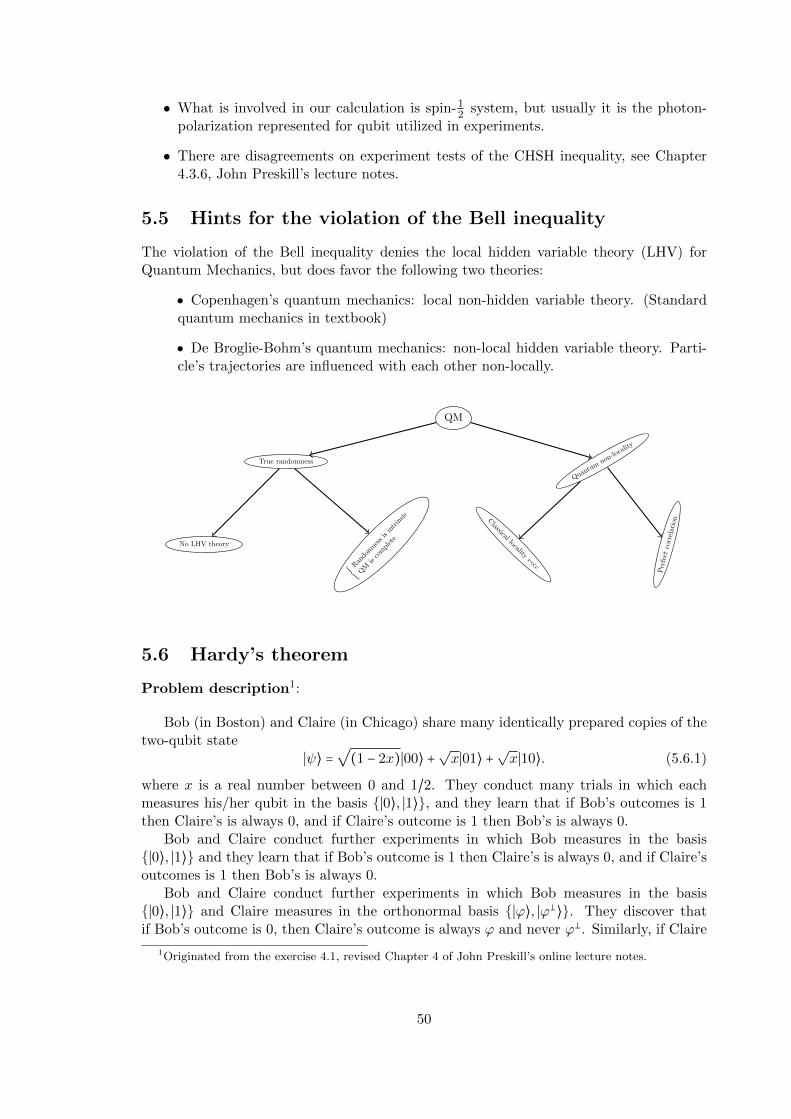
• What is involved in our calculation is spin-12 system, but usually it is the photon-
polarization represented for qubit utilized in experiments.
• There are disagreements on experiment tests of the CHSH inequality, see Chapter4.3.6, John Preskill’s lecture notes.
5.5 Hints for the violation of the Bell inequality
The violation of the Bell inequality denies the local hidden variable theory (LHV) forQuantum Mechanics, but does favor the following two theories:
Copenhagen’s quantum mechanics: local non-hidden variable theory. (Standardquantum mechanics in textbook)
De Broglie-Bohm’s quantum mechanics: non-local hidden variable theory. Parti-cle’s trajectories are influenced with each other non-locally.
QM
True randomness
Quantumnon-lo
cality
No LHV theory
Ran
dom
ness
isin
trin
sic
QM
isco
mpl
ete
Classical locality
v≪c
Per
fect
corr
elat
ion
5.6 Hardy’s theorem
Problem description1:
Bob (in Boston) and Claire (in Chicago) share many identically prepared copies of thetwo-qubit state
∣ψ⟩ =√
(1 − 2x)∣00⟩ +√x∣01⟩ +
√x∣10⟩. (5.6.1)
where x is a real number between 0 and 1/2. They conduct many trials in which eachmeasures his/her qubit in the basis ∣0⟩, ∣1⟩, and they learn that if Bob’s outcomes is 1then Claire’s is always 0, and if Claire’s outcome is 1 then Bob’s is always 0.
Bob and Claire conduct further experiments in which Bob measures in the basis∣0⟩, ∣1⟩ and they learn that if Bob’s outcome is 1 then Claire’s is always 0, and if Claire’soutcomes is 1 then Bob’s is always 0.
Bob and Claire conduct further experiments in which Bob measures in the basis∣0⟩, ∣1⟩ and Claire measures in the orthonormal basis ∣ϕ⟩, ∣ϕ⟩. They discover thatif Bob’s outcome is 0, then Claire’s outcome is always ϕ and never ϕ. Similarly, if Claire
1Originated from the exercise 4.1, revised Chapter 4 of John Preskill’s online lecture notes.
50

measures in the basis ∣0⟩, ∣1⟩ and Bob measures in the basis ∣ϕ⟩, ∣ϕ⟩, then if Claire’soutcome is 0, Bob’s outcome is always ϕ and never ϕ.
Bob and Claire now wonder what will happen if they both measure in the basis∣ϕ⟩, ∣ϕ⟩. Their friend Albert, a firm believer in local realism predicts that it is impos-sible for both to obtain the outcome ϕ(a prediction knows as Hardy’s theorem). Albertargues as follows:
When both Bob and Claire measures in the basis ∣ϕ⟩, ∣ϕ⟩, it is reasonable toconsider what might have happened if one or the other had measured in the basis∣0⟩, ∣1⟩ instead.
So suppose that Bob and Claire both measure in the basis ∣ϕ⟩, ∣ϕ⟩, and that theyboth obtain the outcome ϕ, Now if Bob had measured in the basis ∣0⟩, ∣1⟩ instead,we can be certain that his outcome would have been 1, since experiment has shownthat if Bob had obtain 0 then Claire could not have obtained ϕ. Similarly, if Clairehad measured in the basis ∣0⟩, ∣1⟩, then she certainly would have obtained theoutcome 1. We conclude that if Bob and Claire both measured in the basis ∣0⟩, ∣1⟩,both would have obtained the outcome 1. Bit this a contradiction, for experimenthas shown that it is not possible for both Bob and Claire to obtain the outcome 1 ifthey both measure in the basis ∣0⟩, ∣1⟩.
We are therefore forced to conclude that if Bob and Claire both measure in the basis∣ϕ⟩, ∣ϕ⟩, it is impossible for both to obtain the outcome ϕ.
Though impressed by Albert’s reasoning, Bob and Claire decide to investigate whatprediction can be inferred from quantum mechanics.
(a) Express the basis ∣ϕ⟩, ∣ϕ⟩ in terms of the basis ∣0⟩, ∣1⟩.
(b) If Bob and Claire both measure in the basis ∣ϕ⟩, ∣ϕ⟩, what is the quantum-mechanical prediction for the probability P (x) that both obtain the outcome ϕ?
(c) Find the ”maximal violation” of Hardy’s theorem: show that the maximal value ofP (x) is P [(3 −
√5)/2] = (5
√5 − 11)/2 ≈ .0902.
(d) Bob and Claire conduct an experiment that confirms the prediction of quantummechanics. What was wrong with Albert’s reasoning?
1) Motivation: Hardy’s theorem is able to make a suitable judgement on the conflictbetween the local hidden variable model and standard quantum mechanics, as well asthe Bell inequalities do.
2) In local hidden variable model, Bob and Charlie are space-like separated and perfectcorrelated.
Bob Charlie
The Box represents for the hidden variable that correlates Bob and Charlie.
• The observables ub and uc satisfy the experimental fact:
ubuc = 0, (5.6.2)
where ub, uc = 0,1.
51

• The observables wb and wc satisfy the experimental facts:
ub = 0 Ô⇒ wc = 0; (5.6.3)
uc = 0 Ô⇒ wb = 0. (5.6.4)
Conclusion:ubuc = 0Ô⇒ ub = 0 or uc = 0Ô⇒ wb = 0 or wc = 0. (5.6.5)
Therefore,Prob(wb ≠ 0 & wc ≠ 0∣ubuc = 0) LHV = 0, (5.6.6)
namelyProb(wb = 1 & wc = 1∣ubuc = 0) LHV = 0. (5.6.7)
In following, we will calculate it in quantum mechanics, and verify
Prob(wb = 1 & wc = 1∣ubuc = 0) QM ≠ 0. (5.6.8)
3) In quantum mechanics, Bob and Charlie are correlated by entangled state ∣ψ⟩BC .
∣ψ⟩BCBob Charlie
∣ψ⟩BC = ∣ϕ⟩B ∣0⟩C +√x∣0⟩B ∣1⟩C
= ∣0⟩B ∣ϕ⟩C +√x∣1⟩B ∣0⟩C
=√
1 − 2x∣00⟩BC +√x∣01⟩BC +
√x∣10⟩BC (5.6.9)
where 0 < x < 12 .
• The observables ub and uc (ub, uc = 0,1) are corresponding to the measurementsUUU b and UUU c defined as
UUU b = ∣0⟩B⟨0∣, UUU ′b = ∣1⟩B⟨1∣, (5.6.10)
UUU c = ∣0⟩C⟨0∣, UUU ′c = ∣1⟩C⟨1∣. (5.6.11)
Note thatUUU b +UUU ′
b = 112, UUU c +UUU ′c = 112. (5.6.12)
The value ub,c = 0 or ub,c = 1 is associated with the measurement result UUU b,c orUUU ′b,c respectively. We have ubuc = 0, because state ∣ψ⟩BC does not have the term
∣11⟩BC .
• The observables wb and wc (wb,wc = 0,1) are corresponding to the measurementsWWW b and WWW c defined as
WWW b = ∣ϕ⟩B⟨ϕ∣, WWW ′b = ∣ϕ⟩B⟨ϕ∣, (5.6.13)
WWW c = ∣ϕ⟩C⟨ϕ∣, WWW ′c = ∣ϕ⟩C⟨ϕ∣, (5.6.14)
where state ∣ϕ⟩ is the normalized state ∣ϕ⟩ defined in (5.6.9), and state ∣ϕ⟩ isorthogonal to the state ∣ϕ⟩. Note that
WWW b +WWW ′b = 112, WWW c +WWW ′
c = 112. (5.6.15)
The value wb,c = 0 or wb,c = 1 is associated with the measurement result WWW b,c orWWW ′
b,c respectively.
52
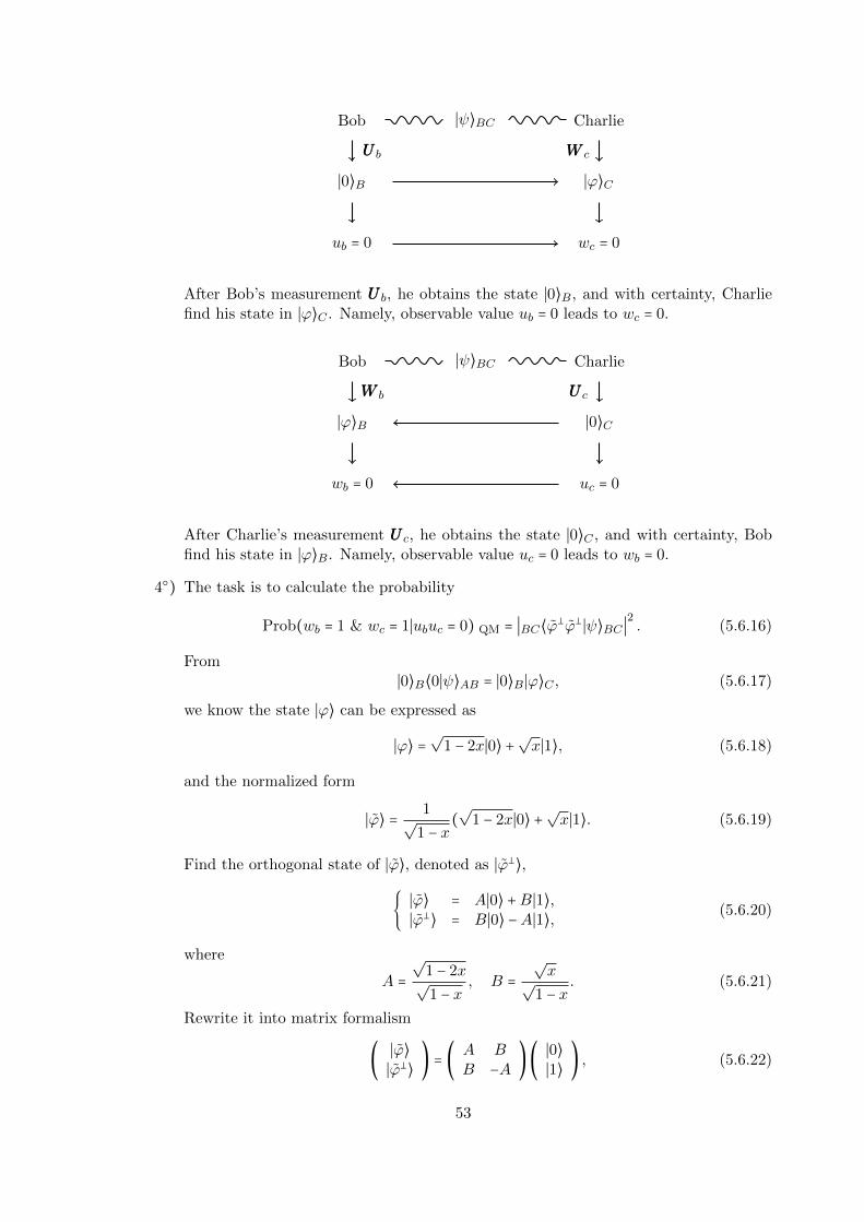
∣ψ⟩BCBob Charlie
UUU b
∣0⟩B
ub = 0
WWW c
∣ϕ⟩C
wc = 0
After Bob’s measurement UUU b, he obtains the state ∣0⟩B, and with certainty, Charliefind his state in ∣ϕ⟩C . Namely, observable value ub = 0 leads to wc = 0.
∣ψ⟩BCBob Charlie
WWW b
∣ϕ⟩B
wb = 0
UUU c
∣0⟩C
uc = 0
After Charlie’s measurement UUU c, he obtains the state ∣0⟩C , and with certainty, Bobfind his state in ∣ϕ⟩B. Namely, observable value uc = 0 leads to wb = 0.
4) The task is to calculate the probability
Prob(wb = 1 & wc = 1∣ubuc = 0) QM = ∣BC⟨ϕϕ∣ψ⟩BC ∣2. (5.6.16)
From∣0⟩B⟨0∣ψ⟩AB = ∣0⟩B ∣ϕ⟩C , (5.6.17)
we know the state ∣ϕ⟩ can be expressed as
∣ϕ⟩ =√
1 − 2x∣0⟩ +√x∣1⟩, (5.6.18)
and the normalized form
∣ϕ⟩ = 1√1 − x
(√
1 − 2x∣0⟩ +√x∣1⟩. (5.6.19)
Find the orthogonal state of ∣ϕ⟩, denoted as ∣ϕ⟩,
∣ϕ⟩ = A∣0⟩ +B∣1⟩,∣ϕ⟩ = B∣0⟩ −A∣1⟩, (5.6.20)
where
A =√
1 − 2x√1 − x
, B =√x√
1 − x. (5.6.21)
Rewrite it into matrix formalism
( ∣ϕ⟩∣ϕ⟩ ) = ( A B
B −A )( ∣0⟩∣1⟩ ) , (5.6.22)
53

where the transformation matrix is a real orthogonal matrix, namely
( A BB −A )( A B
B −A ) = ( A2 +B2 00 B2 +A2 ) = ( 1 0
0 1) . (5.6.23)
Therefore,
( ∣0⟩∣1⟩ ) = ( A B
B −A )( ∣ϕ⟩∣ϕ⟩ ) , (5.6.24)
∣0⟩ = A∣ϕ⟩ +B∣ϕ⟩,∣1⟩ = B∣ϕ⟩ −A∣ϕ⟩. (5.6.25)
Consider the term ∣ϕ⟩A∣ϕ⟩B solely in state ∣ψ⟩AB:
∣00⟩AB ∝ B2∣ϕ⟩A∣ϕ⟩B; (5.6.26)
∣01⟩AB ∝ −AB∣ϕ⟩A∣ϕ⟩B; (5.6.27)
∣10⟩AB ∝ −AB∣ϕ⟩A∣ϕ⟩B. (5.6.28)
Hence
∣ψ⟩AB ∝ (√
1 − 2xB2 − 2√xAB)∣ϕϕ⟩BC = −
√1 − 2x
x
1 − x∣ϕϕ⟩BC . (5.6.29)
Prob(wb = 1 & wc = 1∣ubuc = 0) QM = ∣BC⟨ϕϕ∣ψ⟩BC ∣2
= (1 − 2x) x2
(1 − x)2
= p(x). (5.6.30)
Find the maximal value of function p(x):
p′(x) = 2x
(1 − x)3(x2 − 3x + 1) = 0. (5.6.31)
And
x± =3 ±
√5
2, x0 = 0. (5.6.32)
Due to 0 < x < 12 , we have
pmax(x−) =5√
5 − 11
2≈ 0.0902 ≠ 0. (5.6.33)
The result is conflicted with local hidden variable theory.
5) Reason for conflict between quantum mechanics and local hidden variable theory:
[UUU b,WWW b] ≠ 0, [UUU c,WWW c] ≠ 0. (5.6.34)
Due to uncertainty relation, ub, wb and uc, wc can not be determined simultaneously.
Note:[XXX,ZZZ] ≠ 0⇏ [XXX ⊗XXX,ZZZ ⊗ZZZ] = 0. (5.6.35)
54

Table 5.3: A comparison between Bell’s inequalities, Hardy’s theorem and GHZ theorem
Parties Formalism Correlation Statement
Bell inequalities 2 Inequality Statistical
Hardy’s theorem 2 Equality Statistical LHV hypothesis is denied
GHZ theorem 3 Equality Perfect
5.7 The GHZ theorem
1) A comparison between Bell’s inequalities, Hardy’s theorem and GHZ theorem is shownin Table 5.3.
2) GHZ theorem (the 3-qubit system)
Step I: Alice, Bob and Charlie are space-like from each other and share the GHZstate, i.e.,
∣GHZ⟩3 =1√2( ∣000⟩ + ∣111⟩ ), (5.7.1)
as shown in the diagram formalism in Figure 5.5.
Alice(I) Bob(II)
Charlie(III)
∣GHZ⟩
Figure 5.5: 3-qubit GHZ state.
Step II: Chose four observables with the form of
AAA ∶=σσσ(1)x σσσ(2)y σσσ(3)y ; (5.7.2a)
BBB ∶=σσσ(1)y σσσ(2)x σσσ(3)y ; (5.7.2b)
⎧⎪⎪⎪⎪⎪⎪⎪⎪⎨⎪⎪⎪⎪⎪⎪⎪⎪⎩
CCC ∶=σσσ(1)y σσσ(2)y σσσ(3)x ; (5.7.2c)
DDD ∶=σσσ(1)x σσσ(2)x σσσ(3)x . (5.7.2d)
For these four observables, we may notice the following things:
• AAA2 =BBB2 =CCC2 =DDD2 = III8;
• AAA,BBB,CCC,DDD are mutually commutative;
• ABCDABCDABCD = −III8;
• DDD =XXX1XXX2XXX3, i.e. phase-bit operator,−ADADAD = −(σσσx)2⊗(σσσyσσσx)⊗(σσσyσσσx) = III2⊗ZZZ⊗ZZZ, i.e. the second parity-bit operator,−CDCDCD = −(σσσyσσσx)⊗(σσσyσσσx)⊗(σσσx)2 = ZZZ⊗ZZZ⊗III2, i.e. the first parity-bitoperator;
55

•
AAA ∣GHZ⟩3=− ∣GHZ⟩3 , (5.7.3a)
BBB ∣GHZ⟩3=− ∣GHZ⟩3 , (5.7.3b)
⎧⎪⎪⎪⎪⎪⎪⎪⎪⎨⎪⎪⎪⎪⎪⎪⎪⎪⎩
CCC ∣GHZ⟩3=− ∣GHZ⟩3 , (5.7.3c)
DDD ∣GHZ⟩3= ∣GHZ⟩3 , (5.7.3d)
since
AAA=XXX1⊗(−iZZZ2XXX2)⊗(−iZZZ3XXX3)=−XXX1⊗(ZZZ2XXX2)⊗(ZZZ3XXX3),BBB=(−iZZZ1XXX1)⊗XXX2⊗(−iZZZ3XXX3)=−(ZZZ1XXX1)⊗XXX2⊗(ZZZ3XXX3),
⎧⎪⎪⎪⎪⎪⎪⎪⎪⎨⎪⎪⎪⎪⎪⎪⎪⎪⎩
CCC=(−iZZZ1XXX1)⊗(−iZZZ2XXX2)⊗XXX3=−(ZZZ1XXX1)⊗(ZZZ2XXX2)⊗XXX3,
DDD=XXX1⊗XXX2⊗XXX3.
Step III: For LHV hypothesis, A,B,C,D can be exactly determined, i.e.
A=m(1)x m(2)y m(3)y ; (5.7.4a)
B=m(1)y m(2)x m(3)y ; (5.7.4b)
⎧⎪⎪⎪⎪⎪⎪⎪⎪⎨⎪⎪⎪⎪⎪⎪⎪⎪⎩
C=m(1)y m(2)y m(3)x ; (5.7.4c)
D=m(1)x m(2)x m(3)x ; (5.7.4d)
withm(i)x ,m(j)y = ±1, i, j = 1,2,3 . (5.7.5)
Thus,
ABCD = (m(1)x m(1)y m(2)x m(2)y m(2)y m(2)x )2
= 1. (5.7.6)
Step IV: While for QM, we can get from E.Q.(5.7.3a)∼(5.7.3d) that
ABCDABCDABCD ∣GHZ⟩ = − ∣GHZ⟩ , (5.7.7)
i.e.ABCD = −1. (5.7.8)
Step V: Experiment support E.Q.(5.7.8), which means LHV is denied.
Remark: In QM, [σσσ(i)x ,σσσ(i)y ] ≠ 0, with i = 1,2,3, thus m
(i)x and m
(i)y
cannot be determined simultaneously.
56

Part II
Quantum Computing andQuantum Algorithm
57

Chapter 6
Classical Circuit and QuantumCircuit
Computers are physical objects, and computations are physical processes.What computers can or can not compute is determined by the laws of physicsalone, and not by pure mathematics.
—David Deutsch
By raising these issues we wish to introduce the question of the completenessof the quantum circuit model, and reemphasize the fundamental point thatinformation is physical.
—Nielsen & Chuang
Whether physically reasonable models of computation exist, which beyond thequantum circuit model is a fascinating question which we leave open for you.
—Nielsen & Chuang
A detailed examination and attempted justification of the physics underlyingthe quantum circuit model is outside of the scope of the present discussions,and indeed outside the scope of the present knowledge.
—Nielsen & Chuang
In our attempts to formulate the models of information processing, we shouldalways attempt to go back to fundamental physical laws.
—Nielsen & Chuang
Reference:
[Preskill] New Chapter 5: Classical circuit and quantum circuit;
[Nielsen & Chuang] Chapter 3: Introduction to computer science;
[Nielsen & Chuang] Chapter 4: Quantum circuits.
6.1 Classical circuit
Def 6.1.1. Classical circuit, a circuit model of classical computation, is a finite sequenceof elementary gates applied to a finite string of input bits.
58

6.1.1 Universal gate set
6.1.1.1 Elementary logical gates
(1) NOT gate:NOT ∶ x ↦ x = 1 − x, (6.1.1)
from which we shall see thatNOTNOT = Id, (6.1.2)
i.e. “NOT” gate is a reversible gate. The truth table of the NOT gate is shown inTable 6.1.
Table 6.1: Truth table of NOT gate.
input output
0 1
1 0
(2) AND gate:AND ∶ (x, y) ↦ (x⋅y) mod 2 = x ∧ y. (6.1.3)
The “AND” gate is irreversible. Its truth table is Table 6.2.
Table 6.2: Truth table of AND gate.
input output
0 0 0
0 1 0
1 0 0
1 1 1
(3) OR gate:OR ∶ (x, y) ↦ x + y − xy = x ∨ y. (6.1.4)
As we can see that “OR” gate is irreversible. The corresponding truth table is Table6.3.
Table 6.3: Truth table of OR gate.
input output
0 0 0
0 1 1
1 0 1
1 1 1
59

6.1.1.2 Universal gate set
Def 6.1.2. An universal gate is a finite set of elementary gates which suffice to evaluateany function of a finite number of input bits.
Note: For a general function:
general function F ∶ 0,1n↦0,1n
typical function fi ∶ 0,1n↦0,1
⎫⎪⎪⎬⎪⎪⎭⇒ F = (f1, f2,⋯, fn),
i.e., the general function can be represented by typical functions.Examples:
• Thm1: NOT,AND is an universal gate set;
• Thm2: NOT,OR is an universal gate set;
• Thm3: NAND,COPY is an universal gate set;
Remark:NAND ∶=NOTAND, (6.1.5)
andCOPY ∶ x ↦ (x,x). (6.1.6)
Since
NOT(x) = 1 − x = 1 − x2 = 1 −AND(x) = NOTAND(x,x), (6.1.7)
thusNOT(x) = NAND(x,x) = NANDCOPY(x). (6.1.8)
• Thm4: NOR,COPY is an universal gate set.
NOR ∶=NOTOR. (6.1.9)
6.2 Reversible classical computation
6.2.1 Irreversible computation
Classical computation in terms of irreversible gates, such as AND, OR, NAND, NORgates, is irreversible.
Thm 6.2.1.1 (Landauer’s principle). Irreversible logic gates erase information with irre-ducible expenditure of power.
This means that if we want to erase information, we have to pay for it with work (energy),i.e., energy loss. On the other hand, the reversible gates would ensure that there is noexpenditure of power, i.e., there is no energy loss.
Quantum Computer is reversible, which is one of the reasons people prefer QuantumComputer.
60

Table 6.4: Irreversible and reversible computation
Computer Gates Erasure of information
Irreversible Irreversible gates Irreducible expenditure
Reversible Reversible gates No expenditure
6.2.2 Classical reversible gate
One-bit reversible gates:
NOT(x) = 1 − x = x, NOT gate,
Id(x) = x, Identity gate.
Two-bit reversible gate: XOR, i.e., Exclusive OR gate. The quantum analogy of XORis the CNOT gate.
XOR ∶ (x, y) ↦ (x,x⊕y). (6.2.1)
With three XOR gate, we can form a swap gate, which is defined as
SWAP ∶ (x, y) ↦ (y, x). (6.2.2)
And the construction should be
SWAP = XOR12XOR21XOR12. (6.2.3)
And, we can verify that,
XOR12XOR21XOR12(x, y)= XOR12XOR21(x,x⊕y)= XOR12(x⊕x⊕y, x⊕y)= (x⊕x⊕y, x⊕y⊕x⊕x⊕y)= (y, x).
Similarly, the quantum analogy should be
SWAP = CNOT12CNOT21CNOT12, (6.2.4)
with SWAP defined asSWAP ∶ ∣ψ⟩⊗ ∣φ⟩ ↦ ∣φ⟩⊗ ∣ψ⟩ . (6.2.5)
And in quantum circuit model, it has the diagrammatical expression
∣ψ⟩ × ∣φ⟩
∣φ⟩ × ∣ψ⟩Thm 6.2.2.1. One-bit gates and two-bit gates cannot suffice universal classical reversiblecomputation.
61

6.2.3 Three-bit Toffoli gate
Def 6.2.1 (Three-bit Toffoli gate).
Toffoli gate θ(3) ∶ (x, y, z) ↦ (x, y, z⊕xy). (6.2.6)
which can also be shown in the diagram formalism,
x xy y
z z⊕xy.
As we can see from the definition of the 3-bit Toffoli gate, it works as the controlled-controlled NOT gate with two control-bit and one target bit, besides it is a nonlineargate.
Thm 6.2.3.1. The 3-bit Toffoli gate with constant bits is universal for classical reversiblecomputation.
Proof. The strategy is by setting constant bits for the Toffli gate, we can obtain an uni-versal gate set made up of two-bit gates and one-bit gates.
1) Toffli gate with z = 1:
θ(3)(x, y,1)= (x, y,1 − xy)= (x, y,NAND(x, y)), (6.2.7)
here we get the NAND gate;
2) Toffli gate with x = 1, z = 0:
θ(3)(1, y,0)= (1, y,0 + y)= (1, y, y)= (1,COPY(y)), (6.2.8)
the COPY gate for this time;
3) Toffli gate with x = 1:
θ(3)(1, y, z)= (1, y, z⊕y)= (1,XOR(y, z)), (6.2.9)
and we get the XOR gate.
Actually, the NAND gate and COPY gate together can make an universal gate set, hencethey can construct a universal reversible computer, i.e., the 3-bit Toffoli gate with constantbits is universal for classical reversible computation, since the 3-bit Toffli gate is reversible:
[θ(3)]2(x, y, z)
= θ(3)(x, y, z⊕xy)= (x, y, z⊕xy⊕xy)= (x, y, z),
62

namely
[θ(3)]2= Id. (6.2.10)
Remark: To construct given classical gate, one may need the exponential number of θ(3)
gates, which is terrible in practice.
6.2.4 Three-bit Fredkin gate
Def 6.2.2 (Three-bit Fredkin gate). The three bit Fredkin gate is defined as
Fredkin gate ∶ (x, y, z) ↦ (x,xz + xy, xy + xz) (6.2.11)
This definition shows that the three-bit Fredkin gate is nonlinear, too.
Thm 6.2.4.1. The three-bit Fredkin gate with constant bits is universal for classical re-versible computation.
Proof. The strategy is the same as the proof that three-bit Toffoli gate is universal for theclassical reversible computation.
1) Fredkin gate with z = 0:
Fredkin(x, y,0)= (x, xy, xy)= (x, xy,AND(x, y)), (6.2.12)
here we get the AND gate;
2) Fredkin gate with y = 0, z = 1:
Fredkin(x,0,1)= (x,x, x)= (COPY(x),NOT(x)), (6.2.13)
and we obtain here the COPY gate and NOT gate;
3) Fredkin gate with x = 1:
Fredkin(1, y, z)= (1, z, y)= (1,SWAP(y, z)), (6.2.14)
and we get the SWAP gate.
Because the NAND gate can be constructed by using the NOT gate and the AND gate,and the NAND gate and COPY gate can make an universal gate set. Therefore, the AND
63
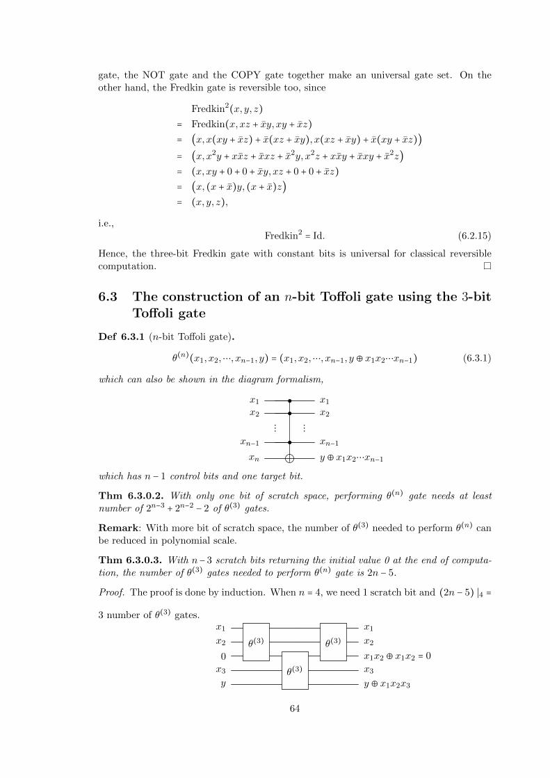
gate, the NOT gate and the COPY gate together make an universal gate set. On theother hand, the Fredkin gate is reversible too, since
Fredkin2(x, y, z)= Fredkin(x,xz + xy, xy + xz)= (x,x(xy + xz) + x(xz + xy), x(xz + xy) + x(xy + xz))= (x,x2y + xxz + xxz + x2y, x2z + xxy + xxy + x2z)= (x,xy + 0 + 0 + xy, xz + 0 + 0 + xz)= (x, (x + x)y, (x + x)z)= (x, y, z),
i.e.,Fredkin2 = Id. (6.2.15)
Hence, the three-bit Fredkin gate with constant bits is universal for classical reversiblecomputation.
6.3 The construction of an n-bit Toffoli gate using the 3-bitToffoli gate
Def 6.3.1 (n-bit Toffoli gate).
θ(n)(x1, x2,⋯, xn−1, y) = (x1, x2,⋯, xn−1, y ⊕ x1x2⋯xn−1) (6.3.1)
which can also be shown in the diagram formalism,
x1 x1
x2 x2
⋮ ⋮xn−1 xn−1
xn y ⊕ x1x2⋯xn−1
which has n − 1 control bits and one target bit.
Thm 6.3.0.2. With only one bit of scratch space, performing θ(n) gate needs at leastnumber of 2n−3 + 2n−2 − 2 of θ(3) gates.
Remark: With more bit of scratch space, the number of θ(3) needed to perform θ(n) canbe reduced in polynomial scale.
Thm 6.3.0.3. With n− 3 scratch bits returning the initial value 0 at the end of computa-tion, the number of θ(3) gates needed to perform θ(n) gate is 2n − 5.
Proof. The proof is done by induction. When n = 4, we need 1 scratch bit and (2n − 5) ∣4 =
3 number of θ(3) gates.x1
θ(3) θ(3)
x1
x2 x2
0
θ(3)x1x2 ⊕ x1x2 = 0
x3 x3
y y ⊕ x1x2x3
64

To prevent possible notation confusion and to maintain the notation consistence in follow-ing, in above quantum circuit diagram, we apply the notation of θ(3) gate as a three-qubitgate. And the new constructed gate functional as the θ(4) gate, we will denote it as θ′(4).Note gate θ′(4) is a 5-bit gate with scratch bit.
Assume we can construct θ(n) gate with n − 3 scratch bits and (2n − 5) number of θ(3)
gates. The gate we have constructed to perform n-bit Toffoli gate is denoted as θ′(n). Inthe manner of recursive construction, to construct θ(n+1) gate, we have
x1
θ(3) θ(3)
x1
x2 x2
0
θ′(n)
0x3 x3
0 0x4 x4
0 0x5 x5
⋮ ⋮xn xny y ⊕ x1x2x3⋯xn
Therefore, the number of scratch space needed to construct θ(n+1) gate is (n − 3) + 1 =(n + 1) − 3. And the number of θ(3) gates is 2n − 5 + 2 = 2(n + 1) − 5.
Thm 6.3.0.4. With n−3 scratch bits returning the initial value at the end of computation,the number of θ(3) gates needed to perform θ(n) gate is 4n − 12.
Proof. When n = 4, we need 1 scratch bit and (4n − 12) ∣4 = 4 number of θ(3) gates.
x1
θ′(4)
x1
x2 x2
s1
θ(3)
s1
x3 x3
y y ⊕ x1x2x3
After the first θ′(4) gate, we have
y′ = y ⊕ (x1x2 ⊕ s1)x3 = y ⊕ x1x2x3 ⊕ s1x3. (6.3.2)
After the second θ(3) gate, we obtain
y′′ = y ⊕ x1x2x3. (6.3.3)
In the case of construction θ(n) gate, we can find we need one θ′(n) gate and one θ′(n−1)
65

gate, shown asx1
θ′(n)
x1
x2 x2
s1
θ′(n−1)
s1
x3 x3
s2 s2
x4 x4
s3 s3
x5 x5
⋮ ⋮xn−1 xn−1
y y ⊕ x1x2x3⋯xn
After the first θ′(n) gate, we have
y′ = y ⊕ ((((x1x2 ⊕ s1)x3 ⊕ s2)x4 ⊕ s3)x5 ⊕⋯)xn−1
= y ⊕ x1x2x3⋯xn−1 ⊕ (((s1x3 ⊕ s2)x4 ⊕ s3)x5 ⊕⋯)xn−1
= y ⊕ x1x2x3⋯xn−1 ⊕ z. (6.3.4)
Note the redundant term z can be rewritten as
z = (((x′1x′2 ⊕ s′1)x′3 ⊕ s′2)x′4 ⊕⋯)x′n−2. (6.3.5)
Therefore, one more θ′(n−1) gate can wipe it out,
y′′ = y′ ⊕ z = y ⊕ x1x2x3⋯xn−1. (6.3.6)
We used totally n − 3 scratch bits and (2n − 5) + (2(n − 1) + 5) = 4n − 12 number of θ(3)
gates here.
6.4 Quantum circuit model
• A Quantum Circuit model is composed of a series of single-qubit-gates SU(2)/U(2)and two-qubit-gates SU(4)/U(4).
• Diagrammatic representation as shown in Figure 6.1.
∣x⟩ UUU ∣y⟩
(a) single-qubit gate
∣x1⟩UUU
∣y1⟩
∣x2⟩ ∣y2⟩(b) two-qubit gate
∣x1⟩
UUU
∣y1⟩
∣x2⟩ ∣y2⟩⋮ ⋮
∣xn⟩ ∣yn⟩(c) n-qubit gate
Figure 6.1: Quantum Circuit Model of single-qubit, two-qubit,and n-qubit gates
66
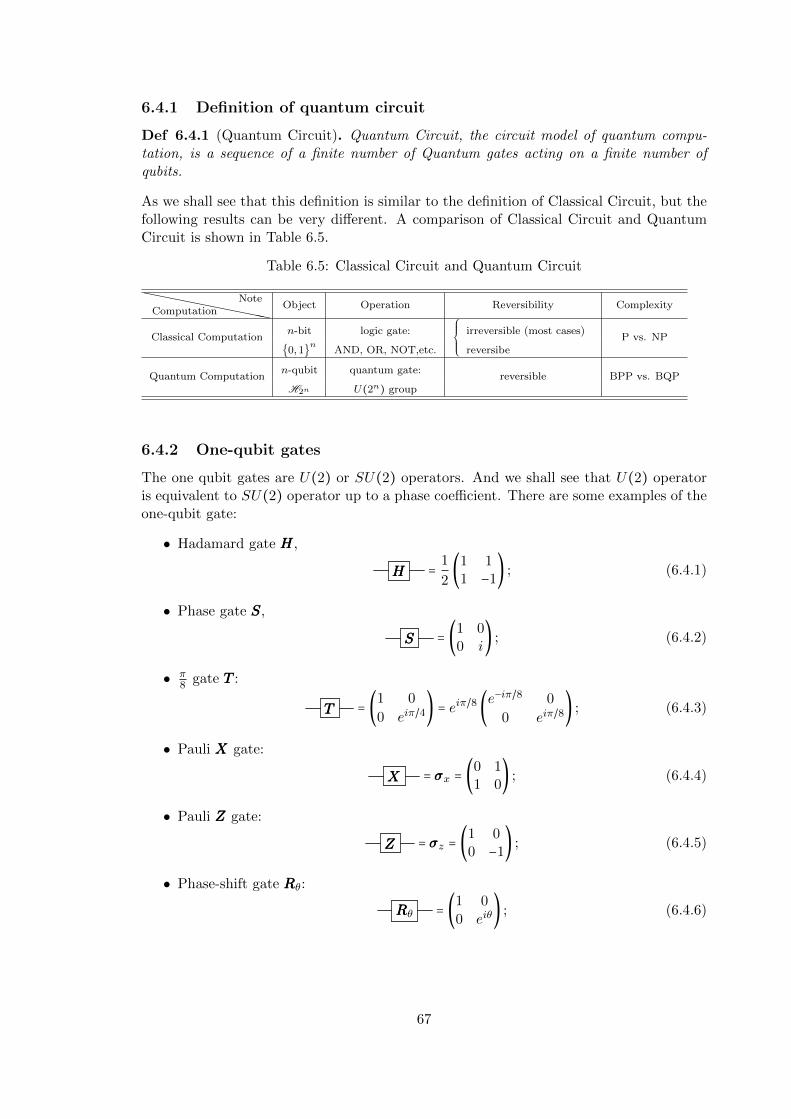
6.4.1 Definition of quantum circuit
Def 6.4.1 (Quantum Circuit). Quantum Circuit, the circuit model of quantum compu-tation, is a sequence of a finite number of Quantum gates acting on a finite number ofqubits.
As we shall see that this definition is similar to the definition of Classical Circuit, but thefollowing results can be very different. A comparison of Classical Circuit and QuantumCircuit is shown in Table 6.5.
Table 6.5: Classical Circuit and Quantum Circuit
`````````ComputationNote
Object Operation Reversibility Complexity
Classical Computationn-bit logic gate:
⎧⎪⎪⎪⎨⎪⎪⎪⎩
irreversible (most cases)
reversibeP vs. NP
0,1n
AND, OR, NOT,etc.
Quantum Computationn-qubit quantum gate:
reversible BPP vs. BQPH2n U(2n) group
6.4.2 One-qubit gates
The one qubit gates are U(2) or SU(2) operators. And we shall see that U(2) operatoris equivalent to SU(2) operator up to a phase coefficient. There are some examples of theone-qubit gate:
• Hadamard gate HHH,
HHH = 1
2(1 1
1 −1) ; (6.4.1)
• Phase gate SSS,
SSS = (1 00 i
) ; (6.4.2)
• π8 gate TTT :
TTT = (1 0
0 eiπ/4) = eiπ/8 (e
−iπ/8 0
0 eiπ/8) ; (6.4.3)
• Pauli XXX gate:
XXX = σσσx = (0 11 0
) ; (6.4.4)
• Pauli ZZZ gate:
ZZZ = σσσz = (1 00 −1
) ; (6.4.5)
• Phase-shift gate RRRθ:
RRRθ = (1 0
0 eiθ) ; (6.4.6)
67
Thm 6.4.2.1. Any U(2) group element can be expressed as
UUU = eiαDDDz(β)DDDy(γ)DDDz(δ), (6.4.7)
where DDDz(β),DDDy(γ), and DDDz(δ) are rotation gates defined as
DDDz(β) ∶= e−iσσσzβ/2=(e−iβ/2 0
0 eiβ/2) , (6.4.8a)
⎧⎪⎪⎪⎪⎪⎪⎪⎪⎪⎪⎪⎪⎪⎪⎨⎪⎪⎪⎪⎪⎪⎪⎪⎪⎪⎪⎪⎪⎪⎩
DDDy(γ) ∶= e−iσσσyγ/2=(cos γ2 − sin γ2
sinγ2 cos γ2) , (6.4.8b)
DDDz(δ) ∶= e−iσσσzδ/2=(e−iδ/2 0
0 eiδ/2) . (6.4.8c)
Proof. Now, we are going to prove the theorem 6.4.2.1 step by step.
Step 1. Any U(2) group element UUU should satisfy the unitary condition
UUUUUU † = UUU †UUU = III2. (6.4.9)
Let’s assume that
UUU ∶= (a′ b′
c′ d′) , with a′, b′, c′, d′ ∈ C. (6.4.10)
From E.Q. (6.4.9) we can get
∣detUUU ∣2 = det (UUUUUU †) = 1,
namelydetUUU = e2iα, with 0 ≤ α < 2π and α ∈ R. (6.4.11)
Step 2. With the E.Q. (6.4.11) in hand, we can denote UUU as
UUU = eiαUUU ′, (6.4.12)
withdetUUU ′ = 1, and UUU ′UUU ′† = UUU ′†UUU ′ = III2, (6.4.13)
and
UUU ′ ∶= (a bc d
) ∈ SU(2), with a, b, c, d ∈ C. (6.4.14)
Thus
(a b)(a∗
b∗)=aa∗ + bb∗=1, (6.4.15a)
(c d)(c∗
d∗)=cc∗ + dd∗=1, (6.4.15b)
⎧⎪⎪⎪⎪⎪⎪⎪⎪⎪⎪⎪⎪⎪⎪⎪⎪⎪⎪⎪⎪⎪⎨⎪⎪⎪⎪⎪⎪⎪⎪⎪⎪⎪⎪⎪⎪⎪⎪⎪⎪⎪⎪⎪⎩
(a b)(c∗
d∗)=ac∗ + bd∗=0, (6.4.15c)
det(a bc d
)= ad − bc =1. (6.4.15d)
Thus, we can conclude that
68

• E.Q.(6.4.15a) and E.Q.(6.4.15b) both can set a constraint on UUU ′, respectively.As we shall see that the imaginary parts of the both two equations are absolutely0.
• E.Q.(6.4.15c) can spell two constraint on UUU ′.
• It seems that E.Q.(6.4.15d) can also put two constraint on UUU ′. But, we canfind out that the constraint (6.4.15d) can be derived from the former threeequations (6.4.15a)∼(6.4.15c).
Therefore, the E.Q.(6.4.15a)∼(6.4.15d) would set totally five constraints on the pa-rameters of UUU ′. Consequently, there are only 8− 5 = 3 degrees of freedom left for theSU(2) group element UUU ′.
Step 3. From the constraint E.Q.(6.4.15c) we can derive
ac∗ + bd∗=0
a∗c + b∗d=0
⎫⎪⎪⎬⎪⎪⎭⇒
⎧⎪⎪⎨⎪⎪⎩
ac∗=−bd∗,a∗c=−b∗d,
namely∣a∣2∣c∣2 = ∣b∣2∣d∣2. (6.4.16)
Combine E.Q.(6.4.15a) and E.Q.(6.4.15b) with E.Q(6.4.16), and we obtain
∣a∣2(1 − ∣d∣2) = (1 − ∣a∣2)∣d∣2,
i.e.,∣a∣ = ∣d∣.
Therefore⎧⎪⎪⎪⎨⎪⎪⎪⎩
∣a∣ = ∣d∣,∣b∣ = ∣c∣,1 = ∣a∣2 + ∣b∣2.
(6.4.17)
Thus,
∣a∣=∣d∣, (6.4.18a)
∣b∣=∣c∣, (6.4.18b)
⎧⎪⎪⎪⎪⎪⎪⎪⎪⎨⎪⎪⎪⎪⎪⎪⎪⎪⎩
1=∣a∣2 + ∣b∣2, (6.4.18c)
0=ac∗ + bd∗, (6.4.18d)
1=ad − bc. (6.4.18e)
Hence, we can denote a, b, c, d in the form of
a=fa cosγ
2, (6.4.19a)
b=−fb sinγ
2, (6.4.19b)
⎧⎪⎪⎪⎪⎪⎪⎪⎪⎪⎪⎪⎪⎨⎪⎪⎪⎪⎪⎪⎪⎪⎪⎪⎪⎪⎩
c=fc sinγ
2, (6.4.19c)
d=fd cosγ
2. (6.4.19d)
69
Step 4. Then, we have
⎧⎪⎪⎪⎪⎨⎪⎪⎪⎪⎩
∣fa∣2 = ∣fb∣2 = ∣fc∣2 = ∣fd∣2 = 1, (6.4.20a)
f∗a fc = f∗b fd, (6.4.20b)
fafd = 1 = fbfc, (6.4.20c)
namely
⎧⎪⎪⎪⎪⎨⎪⎪⎪⎪⎩
∣fa∣ = ∣fb∣ = ∣fc∣ = ∣fd∣ = 1, (6.4.21a)
fc = f∗b , (6.4.21b)
fd = f∗a . (6.4.21c)
Therefore, we can assume that
fa=e−i(β+δ)/2, (6.4.22a)
fb=e−i(β−δ)/2, (6.4.22b)
⎧⎪⎪⎪⎪⎪⎪⎪⎪⎨⎪⎪⎪⎪⎪⎪⎪⎪⎩
fc=ei(β−δ)/2, (6.4.22c)
fd=ei(β+δ)/2, (6.4.22d)
i.e.,
UUU = eiα (e−i(β+δ)/2 cos γ2 −e−i(β−δ)/2 sin γ
2
ei(β−δ)/2 sin γ2 ei(β+δ)/2 cos γ2
)
= eiα (e−iβ 0
0 eiβ/2)(e
−iδ/2 cos γ2 −eiδ/2 sin γ2
e−iδ/2 sin γ2 eiδ/2 cos γ2
)
= eiα (e−iβ 0
0 eiβ/2)(cos γ2 − sin γ
2sin γ
2 cos γ2)(e
−iδ/2 0
0 eδ/2)
= eiαDDDz (β)DDDy (γ)DDDz (δ) . (6.4.23)
Notes:
• Relations between rotations:
DDDy (−π
2)DDDx(α)DDDy (
π
2)=DDDz(α) (6.4.24)⎧⎪⎪⎪⎨⎪⎪⎪⎩DDDz (
π
2)DDDx(α)DDDz (−
π
2)=DDDy(α) (6.4.25)
• Examples:
HHH=DDDx(π)DDDy (π
2)Ph(π
2) , Hadamard gate, (6.4.26)⎧⎪⎪⎪⎨⎪⎪⎪⎩NOT=DDDx(π)Ph(π
2) , NOT gate, (6.4.27)
withPh(θ) ∶= eiθIII2. (6.4.28)
These can be verified easily.
70

– Hadamard gate:
⎧⎪⎪⎪⎪⎪⎨⎪⎪⎪⎪⎪⎩
DDDx(π)=cos(π2) − i sin(π
2)σσσx=−iσσσx,
DDDy (π
2)=cos(π
4) − i sin(π
4)σσσy=
1√2(III2 − iσσσy) ,
from which we can get the left-hand-side of E.Q. (6.4.26)
DDDx(π)DDDy (π
2)Ph(π
2) = 1√
2σσσx (III2 − iσσσy)
= 1√2(σσσx − iσσσxσσσy)
= 1√2(σσσx +σσσz)
= HHH.
– NOT gate X:
DDDx(π)Ph(π2) = (cos
π
2− i sin π
2σσσx) i
= σσσx
= X.
Notes: For an arbitrary single-qubit gate, we exploit the symbol D to denote it, sincesuch the notation is often used to denote the spinor representation of the SU(2) group. Inthe literature, we may use another the symbol R instead of D , since this notation meansthe an arbitrary single-qubit gate may represent a rotation in three dimensional space.
6.4.3 Hadamard gate: HHH
Def 6.4.2 (Hadamard gate).
HHH HHH ∶= 1√2(XXX +ZZZ) = 1√
2(1 1
1 −1) , (6.4.29)
is named as Hadamard gate.
We can easily verify the following relations by utilizing the properties of the Pauli matrices,
HXHHXHHXH = ZZZ; (6.4.30)
HZHHZHHZH = XXX; (6.4.31)
HYHHYHHYH = −YYY ; (6.4.32)
HHH† = HHH; (6.4.33)
HHH2 = III2. (6.4.34)
As we can see that Hadamard gate HHH is not only a unitary transformation but also self-adjoint.
Proof. From the definition (6.4.29) of the Hadamard gate HHH, and the properties of thePauli matrices, we can derive the properties (6.4.30)∼(6.4.34) of the Hadamard gate.
71

(1) For E.Q. (6.4.30), we can evaluate its left-hand-side,
HXHHXHHXH = 1√2(XXX +ZZZ)XXX 1√
2(XXX +ZZZ)
= 1
2(XXX +ZZZ)XXX(XXX +ZZZ)
= 1
2(XXXXXXXXX +ZXXZXXZXX +XXZXXZXXZ +ZXZZXZZXZ)
= 1
2(XXX +ZZZ +ZZZ −XZZXZZXZZ)
= 1
2(XXX +ZZZ +ZZZ −XXX)
= ZZZ,
which is equivalent to the corresponding right-hand-side of E.Q. (6.4.30).
(2) As for E.Q. (6.4.31), we can get in the following manner
HZHHZHHZH = 1√2(XXX +ZZZ)ZZZ 1√
2(XXX +ZZZ)
= 1
2(XXX +ZZZ)ZZZ(XXX +ZZZ)
= 1
2(XZXXZXXZX +ZZXZZXZZX +XZZXZZXZZ +ZZZZZZZZZ)
= 1
2(−ZXXZXXZXX +XXX +XXX +ZZZ)
= 1
2(−ZZZ +XXX +XXX +ZZZ)
= XXX.
(3) We do the same trick as in the former two cases to derive E.Q. (6.4.32),
HYHHYHHYH = 1√2(XXX +ZZZ)YYY 1√
2(XXX +ZZZ)
= 1
2(XXX +ZZZ)YYY (XXX +ZZZ)
= 1
2(XYXXYXXYX +ZY XZY XZY X +XY ZXY ZXY Z +ZY ZZY ZZY Z)
= 1
2(−YYY − i + i −YYY )
= −YYY .
(4) Because the Pauli matricesXXX andZZZ are self-adjoint, therefore should be the Hadamardoperator HHH,
HHH† = 1√2(XXX +ZZZ)†
= 1√2(XXX† +Z†)
= 1√2(XXX +ZZZ)
= HHH.
72

(5) Still from the definition (6.4.29) of the Hadamard gate HHH, we can calculate thesquare of the Hadamard operator HHH,
HHH2 = 1
2(XXX +ZZZ)2
= 1
2(XXX2 +ZZZ2 + XXX,ZZZ)
= 1
2(III2 + III2 + 0)
= III2.
Therefore, we have shown that HHH gate is a self-adjoint unitary 2 × 2 matrix.
In the view point of rotation operator, we have
HHH = 1√2(σσσx +σσσz)
= 1√2(ex + ez) ⋅σ,
namely
HHH = n⋅σσσ, with n ∶= 1√2(ex + ey) ∈ R3. (6.4.35)
Thus,
iHHH = exp (−iθ2n⋅σσσ)∣
θ=π,
which we can put in another way
iHHH =DDD(n, π), (6.4.36)
namely a unitary transformation induced by the rotation along n through angle π in thethree-dimensional Euclidean space. As a matter of fact, the Hadmard gate HHH can make aunitary basis transformations between ZZZ basis and XXX basis:
HHH ∣0⟩ = ∣+⟩ ,HHH ∣1⟩ = ∣−⟩ , (6.4.37)
and
HHH ∣+⟩ = ∣0⟩ ,HHH ∣−⟩ = ∣1⟩ . (6.4.38)
E.Q. (6.4.37) can be easily derived by utilizing the definition (6.4.29) of the Hadamardgate HHH as shown in the following
HHH ∣0⟩ = 1√2(XXX +ZZZ) ∣0⟩
= 1√2(∣1⟩ + ∣0⟩)
= ∣+⟩ ,
and
HHH ∣1⟩ = 1√2(XXX +ZZZ) ∣1⟩
= 1√2(∣0⟩ − ∣1⟩)
= ∣−⟩ .
73

While E.Q. (6.4.38) can be deduced by applying HHH on both sides of E.Q. (6.4.37) andutilizing E.Q. (6.4.34).Furthermore, We can reformulate E.Q. (6.4.37) into one index form, expressed as
HHH ∣i⟩ = 1√2((−1)i ∣i⟩ + ∣i⟩ ), (6.4.39)
where i = 0,1.On the other hand we can also get
⎧⎪⎪⎨⎪⎪⎩
HHH ∣↑y⟩ = 1+i2 ∣↓y⟩ ,
HHH ∣↓y⟩ = 1−i2 ∣↑y⟩ ,
(6.4.40)
also as a consequence of E.Q. (6.4.37)
1√2HHH( ∣0⟩±i ∣1⟩ ) = 1√
2(HHH ∣0⟩±iHHH ∣1⟩ )
= 1√2( ∣+⟩±i ∣−⟩ )
= 1
2( ∣0⟩ + ∣1⟩±i ∣0⟩∓i ∣1⟩ )
= 1
2((1±i) ∣0⟩ + (1∓i) ∣1⟩ )
= 1±i2
( ∣0⟩ + 1∓i1±i
∣1⟩ )
= 1±i2
( ∣0⟩∓i ∣1⟩ ).
6.4.4 Controlled two-qubit gates and controlled three-qubit gates
Def 6.4.3 (Controlled two-qubit gates). Controlled operation is defined as
⎧⎪⎪⎨⎪⎪⎩
if A is true, then do B;
if A is false, then do C.
Controlled operation is essential in computer science.
Def 6.4.4 (Controlled UUU gate). Let’s denote the Controlled UUU gate as CUCUCU , then
CUCUCU ∶ ∣c⟩ ∣t⟩ ↦ ∣c⟩UUU c ∣t⟩ , (6.4.41)
which meansif c = 0, ∣0⟩ ∣t⟩ ↦ ∣0⟩ ∣t⟩ ,if c = 1, ∣1⟩ ∣t⟩ ↦ ∣1⟩UUU ∣t⟩ ,
where ∣c⟩ is the control qubit, and ∣t⟩ is the target qubit. This can also be represented inthe diagrammatical formalism:
CUCUCU =
UUU
One example of the Controlled UUU gate is the CNOT gate, i.e.,
=XXX .
74

6.4.4.1 CNOT gate
Def 6.4.5 (CNOT). The Controlled-Not gate, or CNOT gate for short, is defined as
CNOT ∶ ∣a⟩⊗ ∣b⟩ = ∣a, b⟩↦ ∣a, a⊕b⟩ , a⊕b = (a + b) mod 2, (6.4.42)
where we call ∣a⟩ as the controlled qubit, ∣b⟩ as the target qubit. The CNOT gate is usuallyrepresented with the diagram
∣a⟩ ∣a⟩CNOT ∣ab⟩ =
∣b⟩ ∣b⊕a⟩ .Remarks:
(1) With a = 0, thenCNOT ∣0⟩⊗ ∣b⟩ = ∣0⟩⊗ ∣b⟩ . (6.4.43)
With a = 1, thenCNOT ∣1⟩⊗ ∣b⟩ = ∣1⟩⊗ ∣b⟩ . (6.4.44)
It is the reason why the CNOT gate is called controlled not gate, namely if targetbit is 1, we do the NOT operation.
(2) The controlled-UUU gate is defined as
CUCUCU ∣c⟩ ∣t⟩ ∶= ∣c⟩UUU c ∣t⟩ . (6.4.45)
CUCUCU =
UUU
See more details and properties of the controlled-UUU gate in following section 6.4.4.
(3) From the definition of the CNOT gate, we can verify that
(CNOT)2 = III4, (6.4.46)
since
(CNOT)2 ∣a, b⟩ = CNOT ∣a, b⊕a⟩= ∣a, (b⊕a)⊕a⟩= ∣a, b⟩ ,
with a, b = 0,1.
(4) The CNOT gate can be expressed as
CNOT = ∣0⟩ ⟨0∣⊗III2 + ∣1⟩ ⟨1∣⊗XXX. (6.4.47)
by which we can get the matrix formalism,
CNOT = (1 00 0
)⊗(1 00 1
) + (0 00 1
)⊗(0 11 0
)
namely
CNOT =⎛⎜⎜⎜⎝
11
11
⎞⎟⎟⎟⎠. (6.4.48)
75

(5) CNOT gate is the quantum analogy of the classical gate XOR (the Exclusive ORgate):
⎧⎪⎪⎪⎪⎪⎪⎪⎪⎪⎨⎪⎪⎪⎪⎪⎪⎪⎪⎪⎩
XORXORXOR ∶ (a, b)²2 bits
→ a⊕b±1 bit
, irreversible,
CNOT ∶ (∣a⟩ , ∣b⟩)´¹¹¹¹¹¹¹¹¹¹¹¹¹¸¹¹¹¹¹¹¹¹¹¹¹¹¹¹¶
2 qubits
→ (∣a⟩ , ∣a⊕b⟩)´¹¹¹¹¹¹¹¹¹¹¹¹¹¹¹¹¹¹¹¹¹¹¹¹¸¹¹¹¹¹¹¹¹¹¹¹¹¹¹¹¹¹¹¹¹¹¹¹¹¹¶
2 qubits
, reversible.
(6) CNOT∈SU(4). Since we have derived the matrix formalism, we can see
detCNOT = 1, (6.4.49)
and(CNOT)† = CNOT. (6.4.50)
On the other hand, we know that (CNOT)2 = III4, thus
CNOT(CNOT)† = CNOT(CNOT)† = (CNOT)2 = III4.
Therefore, we can infer that CNOT ∈SU(4).
Lemma 6.4.4.1. The CNOT gate has the following properties
(XXX⊗XXX)CNOT=CNOT(XXX⊗III2), (6.4.51a)
(XXX⊗III2)CNOT=CNOT(XXX⊗XXX), (6.4.51b)
(III2⊗XXX)CNOT=CNOT(III2⊗XXX), (6.4.51c)
⎧⎪⎪⎪⎪⎪⎪⎪⎪⎪⎪⎪⎪⎪⎪⎨⎪⎪⎪⎪⎪⎪⎪⎪⎪⎪⎪⎪⎪⎪⎩
(ZZZ⊗ZZZ)CNOT=CNOT(III2⊗ZZZ), (6.4.51d)
(III2⊗ZZZ)CNOT=CNOT(ZZZ⊗ZZZ), (6.4.51e)
(ZZZ⊗III2)CNOT=CNOT(ZZZ⊗III2). (6.4.51f)
Proof. Now, we are going to verify E.Q.(6.4.51a)∼E.Q.(6.4.51f), one by one, from theexpression (6.4.47) of CNOT gate.
(a) (XXX⊗XXX)CNOT = CNOT(XXX⊗III2)
(XXX⊗XXX)CNOT = (XXX⊗XXX)( ∣0⟩ ⟨0∣⊗III2 + ∣1⟩ ⟨1∣⊗XXX)= XXX ∣0⟩ ⟨0∣⊗XXX +XXX ∣1⟩ ⟨1∣⊗XXX2
= ∣1⟩ ⟨1∣XXX⊗XXXIII2 + ∣0⟩ ⟨0∣XXX⊗III2III2
= ( ∣1⟩ ⟨1∣⊗XXX + ∣0⟩ ⟨0∣⊗III2)(XXX⊗III2)
= CNOT(XXX⊗III2). (6.4.52)
(b) (XXX⊗III2)CNOT = CNOT(XXX⊗XXX)
(XXX⊗III2)CNOT = (XXX⊗III2)( ∣0⟩ ⟨0∣⊗III2 + ∣1⟩ ⟨1∣⊗XXX)= XXX ∣0⟩ ⟨0∣⊗III2 +XXX ∣1⟩ ⟨1∣⊗XXX= ∣1⟩ ⟨1∣XXX⊗XXXXXX + ∣0⟩ ⟨0∣XXX⊗III2XXX
= ( ∣1⟩ ⟨1∣⊗XXX + ∣0⟩ ⟨0∣⊗III2)(XXX⊗XXX)
= CNOT(XXX⊗XXX). (6.4.53)
76

(c) (III2⊗XXX)CNOT = CNOT(III2⊗XXX)
(III2⊗XXX)CNOT = (III2⊗XXX)( ∣0⟩ ⟨0∣⊗III2 + ∣1⟩ ⟨1∣⊗XXX)= ∣0⟩ ⟨0∣⊗XXX + ∣1⟩ ⟨1∣⊗XXX2
= ∣0⟩ ⟨0∣⊗III2XXX + ∣1⟩ ⟨1∣⊗XXXXXX
= ( ∣0⟩ ⟨0∣⊗III2 + ∣1⟩ ⟨1∣⊗XXX)(III2⊗XXX)
= CNOT(III2⊗XXX). (6.4.54)
(d) (ZZZ⊗ZZZ)CNOT = CNOT(III2⊗ZZZ)
(ZZZ⊗ZZZ)CNOT = (ZZZ⊗ZZZ)( ∣0⟩ ⟨0∣⊗III2 + ∣1⟩ ⟨1∣⊗XXX)= ZZZ ∣0⟩ ⟨0∣⊗ZZZ +ZZZ ∣1⟩ ⟨1∣⊗ZXZXZX= ∣0⟩ ⟨0∣⊗ZZZ − ∣1⟩ ⟨1∣⊗(−XZXZXZ)= ∣0⟩ ⟨0∣⊗III2ZZZ + ∣1⟩ ⟨1∣⊗XZXZXZ
= ( ∣0⟩ ⟨0∣⊗III2 + ∣1⟩ ⟨1∣⊗XXX)(III2⊗ZZZ)
= CNOT(III2⊗ZZZ). (6.4.55)
(e) (III2⊗ZZZ)CNOT = CNOT(Z⊗ZZZ)
(III2⊗ZZZ)CNOT = (III2⊗ZZZ)( ∣0⟩ ⟨0∣⊗III2 + ∣1⟩ ⟨1∣⊗XXX)= ∣0⟩ ⟨0∣⊗ZZZ + ∣1⟩ ⟨1∣⊗ZXZXZX= ∣0⟩ ⟨0∣ZZZ⊗III2ZZZ + ∣1⟩ ⟨1∣ZZZ⊗XZXZXZ
= ( ∣0⟩ ⟨0∣⊗III2 + ∣1⟩ ⟨1∣⊗XXX)(ZZZ⊗ZZZ)
= CNOT(ZZZ⊗ZZZ). (6.4.56)
(f) (ZZZ⊗III2)CNOT = CNOT(ZZZ⊗III2)
(ZZZ⊗III2)CNOT = (ZZZ⊗III2)( ∣0⟩ ⟨0∣⊗III2 + ∣1⟩ ⟨1∣⊗XXX)= ZZZ ∣0⟩ ⟨0∣⊗III2 +ZZZ ∣1⟩ ⟨1∣⊗XXX= ∣0⟩ ⟨0∣ZZZ⊗III2
2 + ∣1⟩ ⟨1∣ZZZ⊗XXXIII2
= ( ∣0⟩ ⟨0∣⊗III2 + ∣1⟩ ⟨1∣⊗XXX)(ZZZ⊗III2)
= CNOT(ZZZ⊗III2). (6.4.57)
There we get all the six relations (6.4.51a)∼(6.4.51f) verified.
On the other hand, we can present these properties of the CNOT gate, namely the sixrelations (6.4.51a)∼(6.4.51f), in the form of quantum circuit diagram, which is shown inFigure 6.2.
Lemma 6.4.4.2. The Hadmard gate and CNOT gate have the following connection
(HHH⊗HHH)CNOT12(HHH⊗HHH) = CNOT21, (6.4.58)
with CNOT12 and CNOT21 defined as
CNOT12 ∶ ∣a, b⟩ ↦ ∣a, a⊕b⟩ ,CNOT21 ∶ ∣a, b⟩ ↦ ∣a⊕b, b⟩ . (6.4.59)
77

Proof. The prove is very simple. We can utilize the properties of the Hadmard gate asexpressed in E.Q.(6.4.30)∼(6.4.34) in the following way
(HHH⊗HHH)CNOT12(HHH⊗HHH)
= (HHH⊗HHH)( ∣0⟩ ⟨0∣⊗III2 + ∣1⟩ ⟨1∣⊗XXX)(HHH⊗HHH)
= HHH ∣0⟩ ⟨0∣HHH⊗HHH2 +HHH ∣1⟩ ⟨1∣HHH⊗HXHHXHHXH
= ∣+⟩ ⟨+∣⊗III2 + ∣−⟩ ⟨−∣⊗ZZZ
= ∣+⟩ ⟨+∣⊗( ∣0⟩ ⟨0∣ + ∣1⟩ ⟨1∣ ) + ∣−⟩ ⟨−∣⊗( ∣0⟩ ⟨0∣ − ∣1⟩ ⟨1∣ )
= ( ∣+⟩ ⟨+∣ + ∣−⟩ ⟨−∣ )⊗ ∣0⟩ ⟨0∣ + ( ∣+⟩ ⟨+∣ − ∣−⟩ ⟨−∣ )⊗ ∣1⟩ ⟨1∣
= III2⊗ ∣0⟩ ⟨0∣ +XXX⊗ ∣1⟩ ⟨1∣= CNOT21. (6.4.60)
In this derivation, we have also used the following facts
⎧⎪⎪⎨⎪⎪⎩
CNOT12 = ∣0⟩ ⟨0∣⊗III2 + ∣1⟩ ⟨1∣⊗XXX,CNOT12 = III2⊗ ∣0⟩ ⟨0∣ +XXX⊗ ∣1⟩ ⟨1∣ ,
and⎧⎪⎪⎪⎪⎪⎪⎪⎪⎨⎪⎪⎪⎪⎪⎪⎪⎪⎩
III2 = ∣0⟩ ⟨0∣ + ∣1⟩ ⟨1∣ ,III2 = ∣+⟩ ⟨+∣ + ∣−⟩ ⟨−∣ ,ZZZ = ∣0⟩ ⟨0∣ − ∣1⟩ ⟨1∣ ,XXX = ∣+⟩ ⟨+∣ − ∣−⟩ ⟨−∣ .
And we can also represent the relation (6.4.58) between the Hadmard gate and CNOTgate in the diagram formalism, see Figure 6.3:
XXX XXX=
XXX
(a) (XXX⊗XXX)CNOT = CNOT(XXX⊗III2)
XXX XXX=
XXX
(b) (XXX⊗III2)CNOT = CNOT(XXX⊗XXX)
=XXX XXX
(c) (III2⊗XXX)CNOT = CNOT(III2⊗XXX)
ZZZ =
ZZZ ZZZ
(d) (ZZZ⊗ZZZ)CNOT = CNOT(III2⊗ZZZ)
ZZZ=
ZZZ ZZZ
(e) (III2⊗ZZZ)CNOT = CNOT(ZZZ⊗ZZZ)
ZZZ ZZZ=
(f) (ZZZ⊗III2)CNOT = CNOT(ZZZ⊗III2)
Figure 6.2: Properties of the CNOT gate (6.4.51a)∼(6.4.51f).
78

HHH HHH=
HHH HHH
Figure 6.3: (HHH⊗HHH)CNOT12(HHH⊗HHH) = CNOT21
6.4.4.2 Quantum Toffoli gate and Fredkin gate
Remarks: Quantum Toffoli gate and Fredkin gate can be regarded as controlled-controlled-NOT gate and controlled-swap gate respectively.
Def 6.4.6. Analogy to the classical reversible gate, the Quantum Toffoli gate is defined as
θθθ(3) ∣x, y, z⟩ = ∣x, y, z⊕xy⟩ , (6.4.61)
where x, y, z = 0,1 and it has the diagram formalism,
∣x⟩ ∣x⟩∣y⟩ ∣y⟩∣z⟩ ∣z⊕xy⟩ .
Remark: Quantum Toffoli gate with the Hadamard gate and phase gate is the universalquantum gate set, namely these three gates can perform universal quantum computation.
Def 6.4.7. The Quantum Fredkin gate is defined as
θθθ(3) ∣x, y, z⟩ = ∣x,xz ⊕ xy, xy ⊕ xz⟩ , (6.4.62)
where x, y, z = 0,1 and it has the diagram formalism,
∣x⟩ ∣x⟩∣y⟩ × ∣xz ⊕ xy⟩∣z⟩ × ∣xy ⊕ xz⟩ .
6.4.5 Quantum circuit model of Bell states
Thm 6.4.5.1. With the help of the Hadmard gate and CNOT gate, we can construct theBell state ∣ψ(i, j)⟩ from the product state ∣j, i⟩
∣ψ(i, j)⟩ = CNOT(HHH⊗III2) ∣j, i⟩ , with i, j = 0,1, (6.4.63)
which can also be expressed in the Quantum circuit model
phase-bit ∣j⟩ HHH = ∣ψ(i, j)⟩ .
parity-bit ∣i⟩
Here we present two types of proofs.
Proof. The first type of proof.From the index formulation of the Hadamard gate E.Q. (6.4.39),
(HHH⊗III2) ∣j⟩ ∣i⟩ =1√2((−1)j ∣j⟩ ∣i⟩ + ∣j⟩ ∣i⟩ ). (6.4.64)
79

Following the CNOT gate, we get
CNOT(HHH⊗III2) ∣j⟩ ∣i⟩ =1√2((−1)j ∣j⟩ ∣i⊕ j⟩ + ∣j⟩ ∣i⊕ j⟩ ). (6.4.65)
And considering the case j = 0 and j = 1,
⎧⎪⎪⎪⎨⎪⎪⎪⎩
j = 0 ∶ 1√2( ∣0⟩ ∣i⟩ + ∣1⟩ ∣i⟩ ) = ∣ψ(i,0)⟩
j = 1 ∶ 1√2( ∣0⟩ ∣i⟩ − ∣1⟩ ∣i⟩ ) = ∣ψ(i,1)⟩
(6.4.66)
Conclusively, we haveCNOT(HHH⊗III2) ∣j⟩ ∣i⟩ = ∣ψ(i, j)⟩ . (6.4.67)
Proof. The second type of proof.To prove E.Q.(6.4.63), we may make use of the definition (3.3.2) of the Bell states and
E.Q. (3.3.3). We are going to reach our destination by two main steps.
Step 1: We will prove that ∣ψ(0,0)⟩ = CNOT(HHH⊗III2) ∣00⟩. As we can show that
CNOT(HHH⊗III2) ∣00⟩ = CNOT(HHH ∣0⟩⊗ ∣0⟩ )
= 1√2CNOT( ∣+⟩⊗ ∣0⟩ )
= 1√2CNOT( ∣00⟩ + ∣10⟩ )
= 1√2( ∣00⟩ + ∣11⟩ )
= ∣ψ(0,0)⟩ . (6.4.68)
Step 2: With the equation ∣ψ(i, j)⟩ = (III2⊗XXXiZZZj) ∣ψ(0,0)⟩, we can get
∣ψ(i, j)⟩ = (III2⊗XXXiZZZj) ∣ψ(0,0)⟩
= (III2⊗XXXiZZZj)(CNOT(HHH⊗III2) ∣00⟩ )
= (III2⊗XXX)i(III2⊗ZZZ)jCNOT(HHH⊗III2 ∣00⟩ )
= (III2⊗XXX)iCNOT(ZZZ⊗ZZZ)j(HHH⊗III2 ∣00⟩ )
= CNOT(III2⊗XXX)i(ZZZ⊗ZZZ)j(HHH⊗III2) ∣00⟩ ,
in the last two jumps, we have used the relations (6.4.51e) and (6.4.51c), which wecan verified in the following context:
(III2⊗XXX)iCNOT = (III2⊗XXX)i−1CNOT(I2⊗XXX)⋮= CNOT(III2⊗XXX)i,
and
(III2⊗ZZZ)jCNOT = (III2⊗ZZZ)i−1CNOT(ZZZ⊗ZZZ)⋮= CNOT(ZZZ⊗ZZZ)j .
80
And we should notice that
(III2⊗XXX)i(ZZZj⊗ZZZ)j = ZZZj⊗XXXiZZZj
= (−1)jZZZj⊗XXXi−1ZZZjXXX
⋮= (−1)ijZZZj⊗ZZZjXXXi
= (−1)ij(ZZZj⊗ZZZj)(III2⊗XXXi). (6.4.69)
Thus, we can infer that
∣ψ(i, j)⟩ = (−1)ijCNOT(ZZZj⊗ZZZj)(III2⊗XXXi)(HHH⊗III2) ∣00⟩= (−1)ijCNOT(ZZZj⊗ZZZj)(HHH⊗XXXi) ∣00⟩= (−1)ijCNOT(ZZZj⊗ZZZj)(HHH⊗III2)(III2⊗XXXi) ∣00⟩= (−1)ijCNOT(ZZZj⊗ZZZj)(HHH⊗III2) ∣0i⟩ .
On the other hand, if we’ve noticed that
HZHHZHHZH = XXXHHH2 = III2
⇒ ZHZHZH =HXHXHX, (6.4.70)
then
ZZZjHHH = ZZZj−1HXHXHX
⋮= HXHXHXj . (6.4.71)
Hence,
∣ψ(i, j)⟩ = (−1)ijCNOT(ZZZjHHH⊗ZZZj) ∣0i⟩= (−1)ijCNOT(HXHXHXj⊗ZZZj) ∣0i⟩= (−1)ijCNOT(HHH⊗III2)(XXXj⊗ZZZj) ∣0i⟩= (−1)ijCNOT(HHH⊗III2)(XXXj ∣0⟩⊗ZZZj ∣i⟩)= (−1)ijCNOT(HHH⊗III2)(∣j⟩⊗(−1)ij ∣i⟩)= CNOT(HHH⊗III2) ∣ji⟩ ,
which is equivalent to E.Q. (6.4.63).
6.4.6 Quantum circuit model of GHZ states
Bell states*-HHj
Two-qubit maximally entangled
Most important and popular state
Bell inequality
GHZ states*-HHj
Multi-qubit maximally entangled
Most important and popular state
GHZ theorem
81

Thm 6.4.6.1.
∣GHZ⟩n ∶= 1√2( ∣0x2x3⋯xn⟩ + (−1)x1 ∣1x2x3⋯xn⟩ )
= CNOT1nCNOT1(n−1)⋯CNOT12HHH1 ∣x1x2⋯xn⟩ , (6.4.72)
where CNOTij is the CNOT gate with the i-th qubit as the control qubit and j-th qubitas the target qubit. And this can be represented in the diagram formulism, shown in Figure6.4.
∣x1⟩ HHH
∣x2⟩∣x3⟩
∣GHZ⟩
⋮ ⋮ ⋮ ⋮∣xn⟩
Figure 6.4: ∣GHZ⟩ state generated by the CNOT and H gates.
e.g.1. Three qubit GHZ state.
∣GHZ⟩3 =1√2( ∣000⟩ + ∣111⟩ ). (6.4.73)
∣0⟩
∣0⟩
∣0⟩
HHH
∣GHZ⟩3
t0 t1 t2 t3
Figure 6.5: ∣GHZ⟩3 state generated by the CNOT and H gates.
• t0 ∶ ∣000⟩;
• t1 ∶1√2(∣000⟩ + ∣100⟩);
• t2 ∶1√2(∣000⟩ + ∣110⟩);
• t3 ∶1√2(∣000⟩ + ∣111⟩).
e.g.2. Four qubit GHZ state.
∣GHZ⟩4 =1√2( ∣0011⟩ − ∣1100⟩ ). (6.4.74)
82

∣1⟩
∣0⟩
∣1⟩
∣1⟩
HHH
∣GHZ⟩4
t0 t1 t2 t3 t4
Figure 6.6: ∣GHZ⟩4 state generated by the CNOT and H gates.
• t0 ∶ ∣1011⟩;
• t1 ∶1√2(∣0011⟩ − ∣1011⟩);
• t2 ∶1√2(∣0011⟩ + ∣1111⟩);
• t3 ∶1√2(∣0011⟩ + ∣1101⟩);
• t4 ∶1√2(∣0011⟩ − ∣1100⟩).
Let’s now consider the complete set of observables defining the GHZ state.
• The phase-bit operator XXX1⊗XXX2⊗⋯⊗XXXn:
(XXX1⊗XXX2⊗⋯⊗XXXn)CNOT1nCNOT1(n−1)⋯CNOT12HHH1 ∣x1x2⋯xn⟩= CNOT1n (XXX1⊗XXX2⊗⋯⊗XXXn−1⊗III2)CNOT1(n−1)⋯CNOT12HHH1 ∣x1x2⋯xn⟩= CNOT1nCNOT1(n−1)
(XXX1⊗⋯⊗XXXn−2⊗III2⊗III2)CNOT1(n−2)⋯CNOT12HHH1 ∣x1x2⋯xn⟩⋮= CNOT1nCNOT1(n−1)⋯CNOT12(XXX1⊗III2⊗⋯⊗III2
´¹¹¹¹¹¹¹¹¹¹¹¹¹¹¹¹¹¸¹¹¹¹¹¹¹¹¹¹¹¹¹¹¹¹¹¹¶n−1
)HHH1 ∣x1x2⋯xn⟩
= CNOT1nCNOT1(n−1)⋯CNOT12HHH1(ZZZ1⊗III2⊗⋯⊗III2´¹¹¹¹¹¹¹¹¹¹¹¹¹¹¹¹¹¸¹¹¹¹¹¹¹¹¹¹¹¹¹¹¹¹¹¹¶
n−1
) ∣x1x2⋯xn⟩ ,
i.e.,
(XXX1⊗XXX2⊗⋯⊗XXXn)CNOT1nCNOT1(n−1)⋯CNOT12HHH1 ∣x1x2⋯xn⟩= (−1)x1CNOT1nCNOT1(n−1)⋯CNOT12HHH1 ∣x1x2⋯xn⟩ , (6.4.75)
where we have utilized the relation (6.4.51a), namely
(XXX1⊗XXX2)CNOT12 = CNOT12 (XXX1⊗III2) ,
and the propertyHXHHXHHXH = ZZZ
HHH2 = III2 ⇒ XHXHXH =HZHZHZ.
83

• The first parity-bit operator ZZZ1⊗ZZZ2⊗III2⊗⋯⊗III2´¹¹¹¹¹¹¹¹¹¹¹¹¹¹¹¹¹¸¹¹¹¹¹¹¹¹¹¹¹¹¹¹¹¹¹¹¶
n−2
:
(ZZZ1⊗ZZZ2⊗III2⊗⋯⊗III2´¹¹¹¹¹¹¹¹¹¹¹¹¹¹¹¹¹¸¹¹¹¹¹¹¹¹¹¹¹¹¹¹¹¹¹¹¶
n−2
)CNOT1nCNOT1(n−1)⋯CNOT12HHH1 ∣x1x2⋯xn⟩
= CNOT1nCNOT1(n−1)⋯CNOT13
(ZZZ1⊗ZZZ2⊗III2⊗⋯⊗III2´¹¹¹¹¹¹¹¹¹¹¹¹¹¹¹¹¹¸¹¹¹¹¹¹¹¹¹¹¹¹¹¹¹¹¹¹¶
n−2
)CNOT12HHH1 ∣x1x2⋯xn⟩
= CNOT1nCNOT1(n−1)⋯CNOT12(III2⊗ZZZ2⊗III2⊗⋯⊗III2´¹¹¹¹¹¹¹¹¹¹¹¹¹¹¹¹¹¸¹¹¹¹¹¹¹¹¹¹¹¹¹¹¹¹¹¹¶
n−2
)HHH1 ∣x1x2⋯xn⟩
= CNOT1nCNOT1(n−1)⋯CNOT12HHH1(III2⊗ZZZ2⊗III2⊗⋯⊗III2´¹¹¹¹¹¹¹¹¹¹¹¹¹¹¹¹¹¸¹¹¹¹¹¹¹¹¹¹¹¹¹¹¹¹¹¹¶
n−2
) ∣x1x2⋯xn⟩
= (−1)x2CNOT1nCNOT1(n−1)⋯CNOT12HHH1 ∣x1x2⋯xn⟩ , (6.4.76)
where we have used the relations (6.4.51d) and (6.4.51f), namely
⎧⎪⎪⎨⎪⎪⎩
(ZZZ⊗ZZZ)CNOT12=CNOT12(III2⊗ZZZ),(ZZZ⊗III2)CNOT12=CNOT12(ZZZ⊗III2).
• The second parity-bit III2⊗ZZZ2⊗ZZZ3⊗III2⊗⋯⊗III2´¹¹¹¹¹¹¹¹¹¹¹¹¹¹¹¹¹¸¹¹¹¹¹¹¹¹¹¹¹¹¹¹¹¹¹¹¶
n−3
:
(III2⊗ZZZ2⊗ZZZ3⊗III2⊗III2´¹¹¹¹¸¹¹¹¹¶n−3
)CNOT1nCNOT1(n−1)⋯CNOT12HHH1 ∣x1x2⋯xn⟩
= CNOT1n⋯CNOT14(III2⊗ZZZ2⊗ZZZ3⊗III2⊗III2´¹¹¹¹¸¹¹¹¹¶n−3
)CNOT13CNOT12HHH1 ∣x1x2⋯xn⟩
= CNOT1nCNOT1(n−1)⋯CNOT13
(ZZZ1⊗ZZZ2⊗ZZZ3⊗III2⊗III2´¹¹¹¹¸¹¹¹¹¶n−3
)CNOT12HHH1 ∣x1x2⋯xn⟩
= CNOT1nCNOT1(n−1)⋯CNOT12(III2⊗ZZZ2⊗ZZZ3⊗III2⊗III2´¹¹¹¹¸¹¹¹¹¶n−3
)HHH1 ∣x1x2⋯xn⟩
= CNOT1nCNOT1(n−1)⋯CNOT12HHH1(III2⊗ZZZ2⊗ZZZ3⊗III2⊗III2´¹¹¹¹¸¹¹¹¹¶n−3
) ∣x1x2⋯xn⟩
= (−1)x2+x3CNOT1nCNOT1(n−1)⋯CNOT12HHH1 ∣x1x2⋯xn⟩ , (6.4.77)
to derive this result we have to employ the relations (6.4.51d) and (6.4.51f), i.e.,
⎧⎪⎪⎨⎪⎪⎩
(ZZZ⊗ZZZ)CNOT12=CNOT12(III2⊗ZZZ),(III2⊗ZZZ)CNOT12=CNOT12(ZZZ⊗ZZZ).
84
• The third parity-bit III2⊗III2⊗ZZZ3⊗ZZZ4⊗III2⊗III2´¹¹¹¹¸¹¹¹¹¶n−4
:
(III2⊗III2⊗ZZZ3⊗ZZZ4⊗III2⊗⋯⊗III2´¹¹¹¹¹¹¹¹¹¹¹¹¹¹¹¹¹¸¹¹¹¹¹¹¹¹¹¹¹¹¹¹¹¹¹¹¶
n−4
)CNOT1nCNOT1(n−1)⋯CNOT12HHH1 ∣x1x2⋯xn⟩
= CNOT1n⋯CNOT15
(III2⊗III2⊗ZZZ3⊗ZZZ4⊗III2⊗⋯⊗III2´¹¹¹¹¹¹¹¹¹¹¹¹¹¹¹¹¹¸¹¹¹¹¹¹¹¹¹¹¹¹¹¹¹¹¹¹¶
n−4
)CNOT14CNOT13CNOT12HHH1 ∣x1x2⋯xn⟩
= CNOT1n⋯CNOT14
(ZZZ1⊗III2⊗ZZZ3⊗ZZZ4⊗III2⊗⋯⊗III2´¹¹¹¹¹¹¹¹¹¹¹¹¹¹¹¹¹¸¹¹¹¹¹¹¹¹¹¹¹¹¹¹¹¹¹¹¶
n−4
)CNOT13CNOT12HHH1 ∣x1x2⋯xn⟩
= CNOT1n⋯CNOT13(III2⊗III2⊗ZZZ3⊗ZZZ4⊗III2⊗⋯⊗III2´¹¹¹¹¹¹¹¹¹¹¹¹¹¹¹¹¹¸¹¹¹¹¹¹¹¹¹¹¹¹¹¹¹¹¹¹¶
n−4
)CNOT12HHH1 ∣x1x2⋯xn⟩
= CNOT1n⋯CNOT12HHH1(III2⊗III2⊗ZZZ3⊗ZZZ4⊗III2⊗⋯⊗III2´¹¹¹¹¹¹¹¹¹¹¹¹¹¹¹¹¹¸¹¹¹¹¹¹¹¹¹¹¹¹¹¹¹¹¹¹¶
n−4
) ∣x1x2⋯xn⟩
= (−1)x3+x4CNOT1n⋯CNOT12H1 ∣x1x2⋯xn⟩ . (6.4.78)
• The (n − 1)-th parity-bit III2⊗⋯⊗III2´¹¹¹¹¹¹¹¹¹¹¹¹¹¹¹¹¹¸¹¹¹¹¹¹¹¹¹¹¹¹¹¹¹¹¹¹¶
n−2
⊗ZZZn−1⊗ZZZn:
(III2⊗⋯⊗III2´¹¹¹¹¹¹¹¹¹¹¹¹¹¹¹¹¹¸¹¹¹¹¹¹¹¹¹¹¹¹¹¹¹¹¹¹¶
n−2
⊗ZZZn−1⊗ZZZn)CNOT1nCNOT1(n−1)⋯CNOT12HHH1 ∣x1x2⋯xn⟩
= CNOT1n(ZZZ1⊗III2⊗⋯⊗III2´¹¹¹¹¹¹¹¹¹¹¹¹¹¹¹¹¹¸¹¹¹¹¹¹¹¹¹¹¹¹¹¹¹¹¹¹¶
n−3
⊗ZZZn−1⊗ZZZn)CNOT1(n−1)⋯CNOT12HHH1 ∣x1x2⋯xn⟩
= CNOT1nCNOT1(n−1)
(III2⊗⋯⊗III2´¹¹¹¹¹¹¹¹¹¹¹¹¹¹¹¹¹¸¹¹¹¹¹¹¹¹¹¹¹¹¹¹¹¹¹¹¶
n−2
⊗ZZZn−1⊗ZZZn)CNOT1(n−2)⋯CNOT12HHH1 ∣x1x2⋯xn⟩
= CNOT1n⋯CNOT12HHH1(III2⊗⋯⊗III2´¹¹¹¹¹¹¹¹¹¹¹¹¹¹¹¹¹¸¹¹¹¹¹¹¹¹¹¹¹¹¹¹¹¹¹¹¶
n−2
⊗ZZZn−1⊗ZZZn) ∣x1x2⋯xn⟩
= (−1)xn−1+xnCNOT1n⋯CNOT12HHH1 ∣x1x2⋯xn⟩ . (6.4.79)
6.5 Universal quantum computation
6.5.1 Quantum universal gate set
The definition of the Universal Quantum Gate set is analog to the Universal Classical gateset.
Def 6.5.1 (Universal Quantum Gate set). A set of quantum gates is universal if anyunitary operator UUU ∈ SU(2) (or UUU ∈ U(2), up to a global phase), can be expressed as aproduct of the elementary gates from this very set.
One example of the Universal Quantum Gate set is
CNOT,one-qubit gate ∈ SU(2) .
This is a Universal Quantum Gate set, but the number of the elementary gates in the setis infinity. Thus it is not practical to construct a Quantum Computer with this gate set.
85
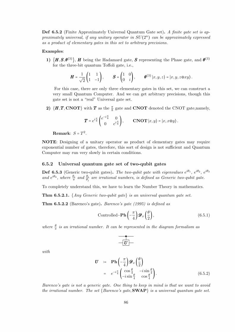
Def 6.5.2 (Finite Approximately Universal Quantum Gate set). A finite gate set is ap-proximately universal, if any unitary operator in SU(2n) can be approximately expressedas a product of elementary gates in this set to arbitrary precisions.
Examples:
1) HHH,SSS,θθθ(3), HHH being the Hadamard gate, SSS representing the Phase gate, and θθθ(3)
for the three-bit quantum Toffoli gate, i.e.,
HHH = 1√2(1 1
1 −1) , SSS = (1 0
0 i) , θθθ(3) ∣x, y, z⟩ = ∣x, y, z⊕xy⟩ .
For this case, there are only three elementary gates in this set, we can construct avery small Quantum Computer. And we can get arbitrary precisions, though thisgate set is not a “real” Universal gate set.
2) HHH,TTT ,CNOT with TTT as the π8 gate and CNOT denoted the CNOT gate,namely,
TTT = eiπ8 (e
−iπ8 0
0 eiπ8) , CNOT ∣x, y⟩ = ∣x,x⊕y⟩ .
Remark: S = T 2.
NOTE: Designing of a unitary operator as product of elementary gates may requireexponential number of gates, therefore, this sort of design is not sufficient and QuantumComputer may run very slowly in certain conditions.
6.5.2 Universal quantum gate set of two-qubit gates
Def 6.5.3 (Generic two-qubit gates). The two-qubit gate with eigenvalues eiθ1, eiθ2, eiθ3
and eiθ4, where θiπ and θi
θjare irrational numbers, is defined as Generic two-qubit gate.
To completely understand this, we have to learn the Number Theory in mathematics.
Thm 6.5.2.1. Any Generic two-qubit gate is an universal quantum gate set.
Thm 6.5.2.2 (Barenco’s gate). Barenco’s gate (1995) is defined as
Controlled−Ph(−π4)DDDx (
θ
2) , (6.5.1)
where θπ is an irrational number. It can be represented in the diagram formalism as
UUU
with
UUU ∶= Ph(−π4)DDDx (
θ
2)
= e−iπ4 ( cos θ4 −i sin θ
4
−i sin θ4 cos θ4
) . (6.5.2)
Barenco’s gate is not a generic gate. One thing to keep in mind is that we want to avoidthe irrational number. The set Barenco’s gate,SWAP is a universal quantum gate set.
86

Thm 6.5.2.3. CNOT,arbitrary single-qubit gates is a universal quantum gate set.
Proof. Since Barenco’s gate together with the SWAP gate can perform universal quantumcomputation, we describe the SWAP gate as
SWAP = CNOT12CNOT23CNOT12, (6.5.3)
and with the following Lemmas, reformulate Barenco’s gate as an expression in terms ofthe CNOT gate and single-qubit gates.
Lemma 6.5.2.1. Any single-qubit gate UUU , can be described in terms of Euler angles,namely
UUU = eiαDDDz(β)DDDy(γ)DDDz(δ), with α,β, γ, δ ∈R. (6.5.4)
Lemma 6.5.2.2. Any single-qubit gate UUU can be formulated as
UUU = Ph (α)AXBXCAXBXCAXBXC, with ABCABCABC = III2, AAA,BBB,CCC ∈ SU(2) and α ∈ R. (6.5.5)
Lemma 6.5.2.3. Any controlled two-qubit gate can be decomposed in the following way
UUU
= RRRα
CCC BBB AAA
(6.5.6)
with
RRRα = (1 00 eiα
) .
Proof. We are now going to prove the three lemmas 6.5.2.1, 6.5.2.2 and 6.5.2.3.
Lemma 1: The lemma 6.5.2.1 is proved in subsection 6.4.2, section 6.4, chapter 6.
Lemma 2: The lemma 6.5.2.2 can be proved through lemma 6.5.2.1. BecauseAAA,BBB,CCCare all elements of the SU(2) group, therefore, from lemma 6.5.2.1, we can constructAAA,BBB,CCC in the form of:
AAA=DDDz(φ)DDDy(ϕ)DDDz(ψ), (6.5.7a)⎧⎪⎪⎪⎪⎨⎪⎪⎪⎪⎩
BBB=DDDz(φ′)DDDy(ϕ′)DDDz(ψ′), (6.5.7b)
CCC=DDDz(φ′′)DDDy(ϕ′′)DDDz(ψ′′), (6.5.7c)
where we have introduced 9 parameters. The expressions (6.5.7a)∼(6.5.7c) ensuresthat AAA, BBB and CCC all belong to SU(2), therefore ABCABCABC ∈ SU(2). Since we can pa-rameterize an arbitrary SU(2) operator with only two independent real variables,the expressions (6.5.7a)∼(6.5.7c) have two constraints. And the relation
ABCABCABC = III2 (6.5.8)
gives rise to another constraint on the parameters that we have introduced in theexpressions (6.5.7a)∼(6.5.7c). Therefore, we actually have 6 independent variablesin the expressions (6.5.7a)∼(6.5.7c). We do not need that much of independent
87
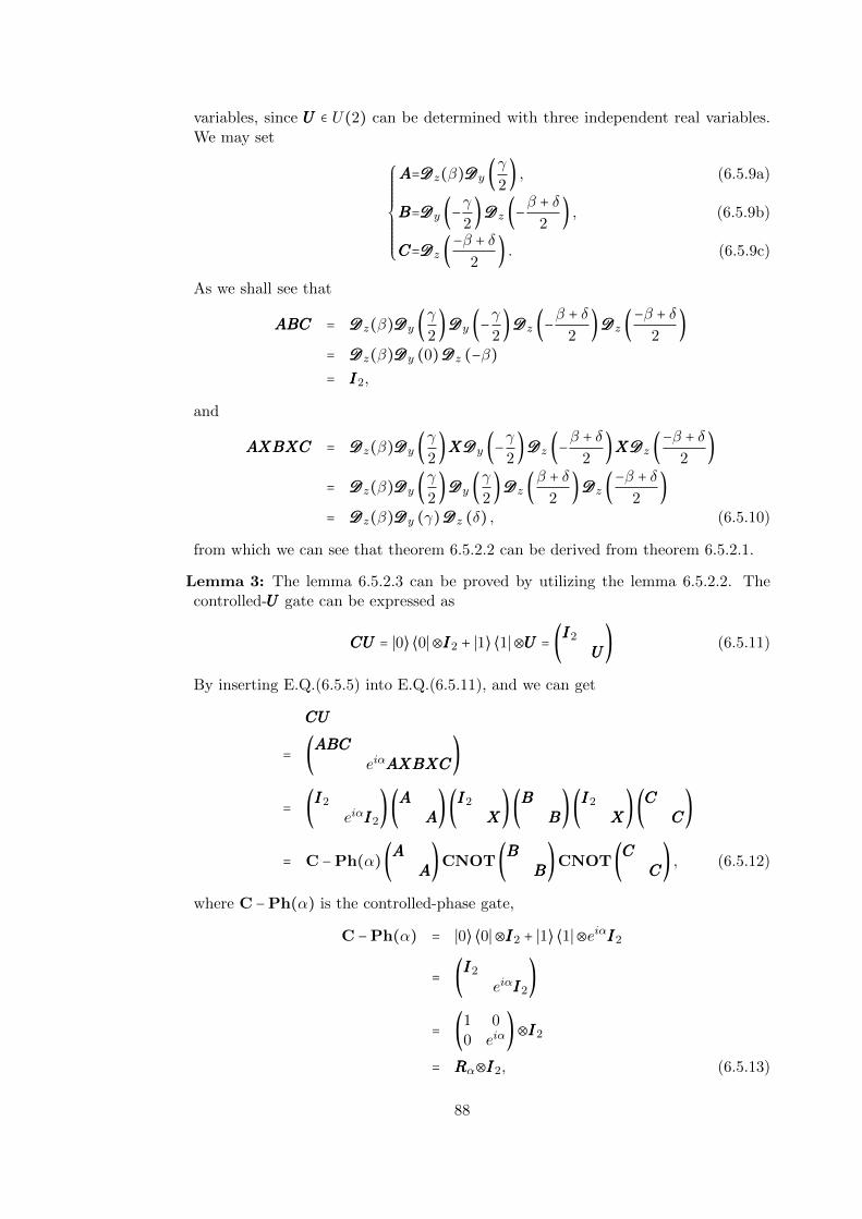
variables, since UUU ∈ U(2) can be determined with three independent real variables.We may set
AAA=DDDz(β)DDDy (γ
2) , (6.5.9a)⎧⎪⎪⎪⎪⎪⎪⎪⎪⎨⎪⎪⎪⎪⎪⎪⎪⎪⎩
BBB=DDDy (−γ
2)DDDz (−
β + δ2
) , (6.5.9b)
CCC=DDDz (−β + δ
2) . (6.5.9c)
As we shall see that
ABCABCABC = DDDz(β)DDDy (γ
2)DDDy (−
γ
2)DDDz (−
β + δ2
)DDDz (−β + δ
2)
= DDDz(β)DDDy (0)DDDz (−β)= III2,
and
AXBXCAXBXCAXBXC = DDDz(β)DDDy (γ
2)XXXDDDy (−
γ
2)DDDz (−
β + δ2
)XXXDDDz (−β + δ
2)
= DDDz(β)DDDy (γ
2)DDDy (
γ
2)DDDz (
β + δ2
)DDDz (−β + δ
2)
= DDDz(β)DDDy (γ)DDDz (δ) , (6.5.10)
from which we can see that theorem 6.5.2.2 can be derived from theorem 6.5.2.1.
Lemma 3: The lemma 6.5.2.3 can be proved by utilizing the lemma 6.5.2.2. Thecontrolled-UUU gate can be expressed as
CUCUCU = ∣0⟩ ⟨0∣⊗III2 + ∣1⟩ ⟨1∣⊗UUU = (III2
UUU) (6.5.11)
By inserting E.Q.(6.5.5) into E.Q.(6.5.11), and we can get
CUCUCU
= (ABCABCABCeiαAXBXCAXBXCAXBXC
)
= (III2
eiαIII2)(AAA
AAA)(III2
XXX)(BBB
BBB)(III2
XXX)(CCC
CCC)
= C −Ph(α)(AAAAAA)CNOT(BBB
BBB)CNOT(CCC
CCC) , (6.5.12)
where C −Ph(α) is the controlled-phase gate,
C −Ph(α) = ∣0⟩ ⟨0∣⊗III2 + ∣1⟩ ⟨1∣⊗eiαIII2
= (III2
eiαIII2)
= (1 00 eiα
)⊗III2
= RRRα⊗III2, (6.5.13)
88
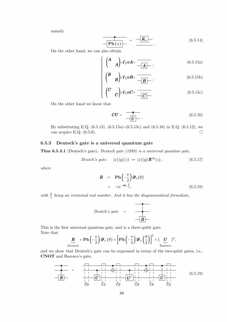
namely
Ph (α)
= RRRα.
(6.5.14)
On the other hand, we can also obtain
(AAAAAA)=III2⊗AAA=
AAA ;(6.5.15a)
⎧⎪⎪⎪⎪⎪⎪⎪⎪⎪⎪⎪⎪⎪⎪⎪⎪⎨⎪⎪⎪⎪⎪⎪⎪⎪⎪⎪⎪⎪⎪⎪⎪⎪⎩
(BBBBBB)=III2⊗BBB=
BBB ;(6.5.15b)
(CCCCCC)=III2⊗CCC=
CCC .(6.5.15c)
On the other hand we know that
CUCUCU = UUU .
(6.5.16)
By substituting E.Q. (6.5.13), (6.5.15a)∼(6.5.15c) and (6.5.16) in E.Q. (6.5.12), wecan acquire E.Q. (6.5.6).
6.5.3 Deutsch’s gate is a universal quantum gate
Thm 6.5.3.1 (Deutsch’s gate). Deutsch gate (1989) is a universal quantum gate,
Deutch’s gate ∶ ∣x⟩ ∣y⟩ ∣z⟩ ↦ ∣x⟩ ∣y⟩RRRxy ∣z⟩ , (6.5.17)
where
RRR ∶= Ph(−π2)DDDx(θ)
= −ie−iσσσxθ2 , (6.5.18)
with θπ being an irrational real number. And it has the diagrammatical formalism,
Deutch’s gate =
RRR
This is the first universal quantum gate, and is a three-qubit gate.Note that
RRR®
Deutsch
= Ph(−π2)DDDx (θ) = [Ph(−π
4)DDDx (
θ
2)]
2
= ( UUU®
Barenco
)2,
and we show that Deutsch’s gate can be expressed in terms of the two-qubit gates, i.e.,CNOT and Barenco’s gate,
=
RRR UUU UUU † UUUt0 t1 t2 t3 t4 t5
(6.5.19)
89
If we let the quantum circuit act on ∣x⟩⊗ ∣y⟩⊗ ∣z⟩ state, then we can get the tripartitestates in different steps as labeled in the right-hand-side of E.Q. (6.5.19):
(1) ∣ψ(t0)⟩ = ∣x⟩ ∣y⟩ ∣z⟩;
(2) ∣ψ(t1)⟩ = ∣x⟩ ∣y⟩UUUy ∣z⟩;
(3) ∣ψ(t2)⟩ = ∣x⟩ ∣x⊕y⟩UUUy ∣z⟩;
(4) ∣ψ(t3)⟩ = ∣x⟩ ∣x⊕y⟩ (UUU †)x⊕yUUUy ∣z⟩= ∣x⟩ ∣x⊕y⟩UUU−x⊕yUUUy ∣z⟩;
(5) ∣ψ(t4)⟩ = ∣x⟩ ∣x⊕y⊕x⟩UUU−x⊕yUUUy ∣z⟩= ∣x⟩ ∣y⟩UUU−x⊕yUUUy ∣z⟩;
(6) ∣ψ(t5)⟩ = ∣x⟩ ∣y⟩UUUxUUU−x⊕yUUUy ∣z⟩= ∣x⟩ ∣y⟩UUUx+y−x⊕y ∣z⟩= ∣x⟩ ∣y⟩UUUx+y−(x+y−2xy) ∣z⟩= ∣x⟩ ∣y⟩UUU2xy ∣z⟩= ∣x⟩ ∣y⟩RRRxy ∣z⟩.
Note: the calculation here is binary, namely
x⊕y ∶= (x + y) mode 2
= x + y − 2xy, (6.5.20)
where x, y ∈ 0,1.
90

Chapter 7
Quantum Algorithms
Quantum mechanics: Real Black Magic Calculus.
—Albert Einstein
Computer programming is an art of form, like the creation of poetry or music.
—Donald Knuth
Deutsch’s algorithm combines quantum parallelism with a property of quantummechanics known as interference.
—Nielsen & Chuang
The quantum search algorithm is essentially optimal, is both exciting anddisappointing. It is exciting because it tells us that for this problem, at least wehave fully plumbed the depths of quantum mechanics, no further improvementis possible. The disappointment arises because we might have hoped to domuch better than the square root speedup offered by the quantum searchalgorithm.
—Nielsen & Chuang
The essence of the design of many quantum algorithms is that a clever choiceof function and final transformation allows efficient determination of usefulglobal information about the function–information which can not be attainedquickly on a classical computer.
—Nielsen & Chuang
Reference:
[Preskill] Chapter 6: Quantum computation;
[Nielsen & Chuang] Chapter 6: Quantum search algorithms
7.1 Classical and quantum algorithm
Def 7.1.1 (Algorithm). An algorithm is
1. a well-defined procedure;
2. with finite descriptions;
91

3. designed for realising an information processing task;
4. designed to solve a computational problem.
This definition is proper for both classical algorithm and quantum algorithm. Theonly thing we have to notice is that, the classical algorithm is designed to process classicalinformation, while the quantum algorithm is designed to perform information processingtask using the fundamental principle’s of Quantum Mechanics.
But, what advantage can we get from the Quantum Algorithm? One of the benefit isthat Quantum Algorithm is more efficient than the Classical Algorithm in some specificproblems. And there are some examples, as shown in Table 7.1:
Table 7.1: Examples of Quantum Algorithm
Speed up Examples
Non-exponential speed up Grover’s search algorithm (Oracle model)
Relativized exponential speed up Simon’s algorithm (Oracle model)
Exponential speed up Shor’s factoring algorithm
7.2 Oracle model
Oracle model is the black-box model.
Def 7.2.1 (Oracle (black box)). A subroutine evaluating a function, but we have no ideaabout how this subroutine is performed. We are only concerned about how this subroutineis performed, or we only make a query, on the Oracle (Black-box).
Remark: For the oracle (black box), usually we don’t care about how the black boxworks, and we are only concerned about how to use it.
• We can make a query on UUUf .
• We are only concerned about the input and output.
• No idea about how UUUf is performed.
Examples:
(1) Classical black box:
x f f(x).
which may be not a reversible operation. And we can define the classical black boxwhich is a reversible gate to compute the function f(x) shown as
xUf
x
y y⊕f(x).
92

(2) Quantum black box is a quantum gate Uf computing f(x):
∣x⟩UUUf
∣x⟩∣y⟩ ∣y⊕f(x)⟩ ,
where ∣x⟩ is called the register qubit, and ∣y⟩ is called the ancilla qubit. Note thatquantum gate UUUf satisfies the unitary (reversible) condition given by
UUU †fUUUf = UUUfUUU
†f = IIId. (7.2.1)
The Query Complexity:
• In the oracle model, we only count the minimal number of the black box to char-acterize the circuit complexity. Because the time of performing UUUf gate takes fargreater than the time of performing other gates.
• Complexity is very abstract, but very important in computer science.
Note: Time of performing UUUf ≫ Time of perform other gates. For example
Time (UUUf) = 1 year;
Time (other gates) = 1 sec. (7.2.2)
7.3 Deutsch’s algorithm
The Deutsch’s algorithm is the first Quantum Algorithm, presented in 1989.
7.3.1 Definitions
Def 7.3.1 (Constant function and Balanced function). Let’s define a function f :
f ∶ ∀x ∈ 0,1 ↦ y = f(x) ∈ 0,1 . (7.3.1)
Then, the function f is
Constant function, if f(0)=f(1); (7.3.2)
Balanced function, if f(0)≠f(1). (7.3.3)
• In the case that f is constant, i.e., f(0) = f(1), we can acquire
f(0) = f(1) = 0, or f(0) = f(1) = 1. (7.3.4)
Therefore,f(0)⊕ f(1) = 0 (7.3.5)
with the binary addition.
• In the case that f is balanced, i.e., f(0) ≠ f(1), we can know
f(0) = 0, f(1) = 1, or f(0) = 1, f(1) = 0. (7.3.6)
Similarly,f(0)⊕ f(1) = 1 (7.3.7)
which suggests that the number of x which satisfies f(x) = 0 and x that f(x) = 1 issame, namely
1 = #x∣f(x) = 0,∀x∈0,1 = #x∣f(x) = 1,∀x∈0,1. (7.3.8)
93
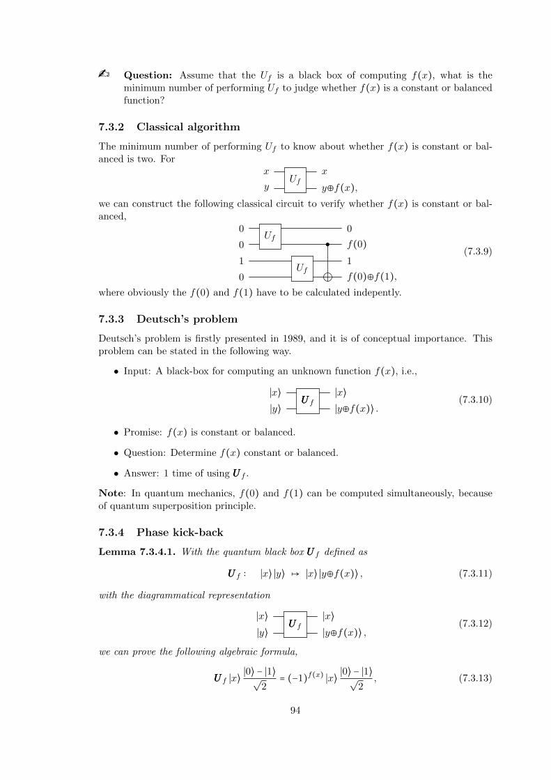
Question: Assume that the Uf is a black box of computing f(x), what is theminimum number of performing Uf to judge whether f(x) is a constant or balancedfunction?
7.3.2 Classical algorithm
The minimum number of performing Uf to know about whether f(x) is constant or bal-anced is two. For
xUf
x
y y⊕f(x),we can construct the following classical circuit to verify whether f(x) is constant or bal-anced,
0Uf
0
0 f(0)1
Uf1
0 f(0)⊕f(1),
(7.3.9)
where obviously the f(0) and f(1) have to be calculated indepently.
7.3.3 Deutsch’s problem
Deutsch’s problem is firstly presented in 1989, and it is of conceptual importance. Thisproblem can be stated in the following way.
• Input: A black-box for computing an unknown function f(x), i.e.,
∣x⟩UUUf
∣x⟩∣y⟩ ∣y⊕f(x)⟩ .
(7.3.10)
• Promise: f(x) is constant or balanced.
• Question: Determine f(x) constant or balanced.
• Answer: 1 time of using UUUf .
Note: In quantum mechanics, f(0) and f(1) can be computed simultaneously, becauseof quantum superposition principle.
7.3.4 Phase kick-back
Lemma 7.3.4.1. With the quantum black box UUUf defined as
UUUf ∶ ∣x⟩ ∣y⟩ ↦ ∣x⟩ ∣y⊕f(x)⟩ , (7.3.11)
with the diagrammatical representation
∣x⟩UUUf
∣x⟩∣y⟩ ∣y⊕f(x)⟩ ,
(7.3.12)
we can prove the following algebraic formula,
UUUf ∣x⟩∣0⟩ − ∣1⟩√
2= (−1)f(x) ∣x⟩ ∣0⟩ − ∣1⟩√
2, (7.3.13)
94

i.e., the quantum circuit model given by
∣x⟩UUUf
∣x⟩
∣0⟩−∣1⟩√
2(−1)f(x) ∣0⟩−∣1⟩√
2.
(7.3.14)
or equivalently
∣x⟩UUUf
(−1)f(x) ∣x⟩
∣0⟩−∣1⟩√
2
∣0⟩−∣1⟩√
2.
(7.3.15)
Note: Why is the above quantum circuit model called the phase kick-back? The glob-al phase (−1)f(x) can be kicked back from the target qubit to the control quibt, so that
the target qubit∣0⟩−∣1⟩√
2seems unchanged from the input to the output.
This lemma can be proved in the following manner.
Proof.
UUUf ∣x⟩∣0⟩ − ∣1⟩√
2=
UUUf ∣x⟩ ∣0⟩ −UUUf ∣x⟩ ∣1⟩√2
= ∣x⟩ ∣f(x)⟩ − ∣x⟩ ∣1⊕f(x)⟩√2
= ∣x⟩ ∣f(x)⟩ − ∣x⟩ ∣f(x)⟩√2
= ∣x⟩ ∣f(x)⟩ − ∣f(x)⟩√2
=⎧⎪⎪⎨⎪⎪⎩
if f(x) = 0, ∣x⟩ 1√2(∣0⟩ − ∣1⟩);
if f(x) = 1, ∣x⟩ 1√2(∣1⟩ − ∣0⟩) = (−1)∣x⟩ 1√
2(∣0⟩ − ∣1⟩);
= (−1)f(x) ∣x⟩ ∣0⟩ − ∣1⟩√2
. (7.3.16)
There we get E.Q. (7.3.13) verified.
Example: If f(x) = x, then UUUx = CNOT, since
UUUx ∣x⟩ ∣y⟩ = ∣x⟩ ∣y⊕f(x)⟩= ∣x⟩ ∣y⊕x⟩= CNOT ∣x⟩ ∣y⟩ . (7.3.17)
And we can see that
CNOT ∣x⟩ ∣0⟩ − ∣1⟩√2
= ∣x⟩ ∣x⟩ − ∣x⟩ ∣x⟩√2
= (−1)x ∣x⟩ ∣0⟩ − ∣1⟩√2
, (7.3.18)
so that in such the circumstance we have CNOT ∣x⟩ = (−1)x ∣x⟩.
Note: The phase kick-back is the key technique in the performance of such quantumalgorithms as Deutsch’s algoithm, Deutsch-Jozsa’a algorithm, Grover’s search algorithm,and so on.
95

7.3.5 Deutsch’s algorithm
This is the first quantum algorithm in quantum information science. Although this al-gorithm may be nonsense in practice, but is of conceptual importance. The associatedquantum circuit is of the form,
0 HHHUUUf
HHH
∣0⟩−∣1⟩√
2t1 t2 t3 t4
(7.3.19)
where we study it in the following five steps:
1. Input: state preparation.
∣ψ(t1)⟩ = ∣0⟩⊗ ∣0⟩−∣1⟩√2,
2. ∣ψ(t2)⟩ = (HHH⊗III2) ∣ψ(t1)⟩
= ∣0⟩+∣1⟩√2⊗ ∣0⟩−∣1⟩√
2,
We have utilized the relation that
HHH ∣0⟩= ∣0⟩ + ∣1⟩√2
HHH ∣1⟩= ∣0⟩ − ∣1⟩√2
⎫⎪⎪⎪⎪⎪⎬⎪⎪⎪⎪⎪⎭
⇐⇒HHH ∣i⟩ = 1√2
1
∑j=0
(−1)i⋅j ∣j⟩ (7.3.20)
where i ⋅ j is AND operation.
3. ∣ψ(t3)⟩ = UUUf ∣ψ(t2)⟩
= 1√2∑1i=0UUUf ∣i⟩⊗
∣0⟩−∣1⟩√
2
= 1√2∑1i=0(−1)f(i) ∣i⟩⊗ ∣0⟩−∣1⟩√
2,
4. ∣ψ(t4)⟩ = (HHH⊗III2) ∣ψ(t3)⟩
= 1√2∑1i=0(−1)f(i)(HHH⊗III2) ∣i⟩⊗ ∣0⟩−∣1⟩√
2
= 12 ∑
1i,j=0(−1)f(i)+i⋅j ∣j⟩⊗ ∣0⟩−∣1⟩√
2.
5. Output: quantum measurement.
And the icon
LL ________
_ _ _ _ _ _ _ _
stands for the measurement with respect to the standard basis∣0⟩ , ∣1⟩. If we perform the measurement ∣0⟩⟨0∣⊗III, there we can get the state aftermeasurement for the bipartite system as,
j = 0 ∶ ∣ψ(t4)⟩ =1
2
1
∑i=0
(−1)f(i) ∣0⟩⊗ ∣0⟩ − ∣1⟩√2
. (7.3.21)
And we can see that,
96

(1) if f is a constant function, i.e., f(0) = f(1), the probability that the first qubitis in the state ∣0⟩ is 1, since
(∣0⟩ ⟨0∣⊗III2) ∣ψ(t4)⟩ = (−1)f(0) ∣0⟩⊗ ∣0⟩ − ∣1⟩√2
, (7.3.22)
(∣1⟩ ⟨1∣⊗III2) ∣ψ(t4)⟩ = 1
2
1
∑i=0
(−1)f(i)+i ∣1⟩⊗ ∣0⟩ − ∣1⟩√2
= (−1)f(0) 12
1
∑i=0
(−1)i ∣1⟩⊗ ∣0⟩ − ∣1⟩√2
= 0; (7.3.23)
(2) if f is a balanced function, i.e., f(0)≠f(1), the probability that the first qubitis in the state ∣0⟩ is 0, due to
(∣0⟩ ⟨0∣⊗III2) ∣ψ(t4)⟩ = 1
2
1
∑i=0
(−1)f(i) ∣0⟩⊗ ∣0⟩ − ∣1⟩√2
= 0. (7.3.24)
Note: What is underlying Deutsch’s algorithm? The f(0) and f(1) are calculatedsimultaneously so that f(0)⊕f(1) is calculated using the black box Uf once. This is calledquantum parallelism due to quantum interference or quantum superposition principle.
7.4 Deutsch-Jozsa’s algorithm
As we have seen that the Deutsch’s algorithm uses the one-qubit register, we are going toconsider the Deutsch-Jozsa’s Algorithm which uses an n-qubit register.
7.4.1 Constant and balanced function in n-qubit
Def 7.4.1 (Constant and Balanced function (n-qubit)). Let’s define the function f to be
f ∶ ∀x ∈ 0,1n ↦ f(x) ∈ 0,1 . (7.4.1)
Then function f is
• Constant function, if f(x) = c, ∀x ∈ 0,1n, where c is a constant in 0,1;
• Balanced function, if the number of elements in the set x∣f(x) = 0,∀x∈0,1n is
the same as that in x∣f(x) = 1,∀x∈0,1n , i.e., the numbers both equal to 2n−1.
#x∣f(x) = 0,∀x∈0,1n = #x∣f(x) = 1,∀x∈0,1n = 2n−1. (7.4.2)
7.4.2 Constant or balanced function?
Question: If we know that f is either a Constant function or a Balanced function,how can we determine it? And, how many queries would have to be made?
There are some optional ways to solve this problem:
97
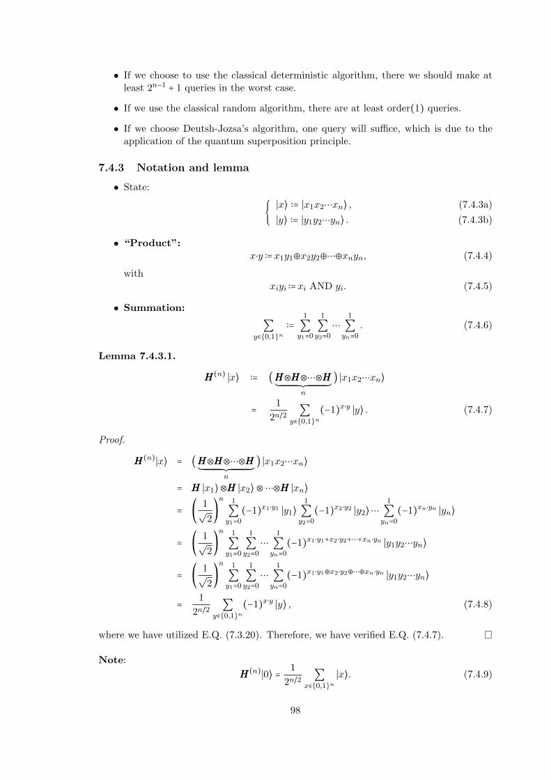
• If we choose to use the classical deterministic algorithm, there we should make atleast 2n−1 + 1 queries in the worst case.
• If we use the classical random algorithm, there are at least order(1) queries.
• If we choose Deutsh-Jozsa’s algorithm, one query will suffice, which is due to theapplication of the quantum superposition principle.
7.4.3 Notation and lemma
• State:
∣x⟩ ∶= ∣x1x2⋯xn⟩ , (7.4.3a)
∣y⟩ ∶= ∣y1y2⋯yn⟩ . (7.4.3b)
• “Product”:x⋅y ∶=x1y1⊕x2y2⊕⋯⊕xnyn, (7.4.4)
withxiyi ∶=xi AND yi. (7.4.5)
• Summation:
∑y∈0,1n
∶=1
∑y1=0
1
∑y2=0
⋯1
∑yn=0
. (7.4.6)
Lemma 7.4.3.1.
HHH(n) ∣x⟩ ∶= (HHH⊗HHH⊗⋯⊗HHH´¹¹¹¹¹¹¹¹¹¹¹¹¹¹¹¹¹¹¹¹¹¹¹¹¹¹¹¹¹¹¹¸¹¹¹¹¹¹¹¹¹¹¹¹¹¹¹¹¹¹¹¹¹¹¹¹¹¹¹¹¹¹¹¹¶
n
) ∣x1x2⋯xn⟩
= 1
2n/2∑
y∈0,1n(−1)x⋅y ∣y⟩ . (7.4.7)
Proof.
HHH(n)∣x⟩ = (HHH⊗HHH⊗⋯⊗HHH´¹¹¹¹¹¹¹¹¹¹¹¹¹¹¹¹¹¹¹¹¹¹¹¹¹¹¹¹¹¹¹¸¹¹¹¹¹¹¹¹¹¹¹¹¹¹¹¹¹¹¹¹¹¹¹¹¹¹¹¹¹¹¹¹¶
n
) ∣x1x2⋯xn⟩
= HHH ∣x1⟩⊗HHH ∣x2⟩⊗⋯⊗HHH ∣xn⟩
= ( 1√2)n 1
∑y1=0
(−1)x1⋅y1 ∣y1⟩1
∑y2=0
(−1)x2⋅y2 ∣y2⟩⋯1
∑yn=0
(−1)xn⋅yn ∣yn⟩
= ( 1√2)n 1
∑y1=0
1
∑y2=0
⋯1
∑yn=0
(−1)x1⋅y1+x2⋅y2+⋯+xn⋅yn ∣y1y2⋯yn⟩
= ( 1√2)n 1
∑y1=0
1
∑y2=0
⋯1
∑yn=0
(−1)x1⋅y1⊕x2⋅y2⊕⋯⊕xn⋅yn ∣y1y2⋯yn⟩
= 1
2n/2∑
y∈0,1n(−1)x⋅y ∣y⟩ , (7.4.8)
where we have utilized E.Q. (7.3.20). Therefore, we have verified E.Q. (7.4.7).
Note:
HHH(n)∣0⟩ = 1
2n/2∑
x∈0,1n∣x⟩. (7.4.9)
98

With the action of the n-fold Hadamard gates, we have the superposition of all the compu-tational basis vectors, namely, all product basis vectors. In other words, all computationalbasis vectors can be encoded in the one quantum state due to the quantum superpositionprinciple.
Lemma 7.4.3.2 (Phase kick-back for n-qubit). Let’s define UUUf as
UUUf ∶ ∣a⟩ ∣y⟩ ↦ ∣a⟩ ∣y⊕f(a)⟩ (7.4.10)
withf ∶ ∀a ∈ 0,1n ↦ f(a)∈0,1 ,
andy ∈ 0,1 .
And we call ∣a⟩ as the first register, which is an n-qubit state, and ∣y⟩ as the second register,which is a single qubit.Therefore,
UUUf ∣x⟩∣0⟩ − ∣1⟩√
2= (−1)f(x) ∣x⟩ ∣0⟩ − ∣1⟩√
2, (7.4.11)
with x ∈ 0,1n. This can also be presented in the diagram formalism:
∣x1⟩
UUUf
∣x1⟩∣x2⟩ ∣x2⟩⋮ ⋮
∣xn⟩ ∣xn⟩∣0⟩−∣1⟩√
2(−1)f(x) ∣0⟩−∣1⟩√
2.
(7.4.12)
Proof.
UUUf ∣x⟩∣0⟩ − ∣1⟩√
2
= ∣x⟩ ∣f(x)⟩ − ∣1 + f(x)⟩√2
= ∣x⟩∣f(x)⟩ − ∣f(x)⟩
√2
= (−1)f(x) ∣x⟩ ∣0⟩ − ∣1⟩√2
. (7.4.13)
We have made use of the same technique exploited to prove lemma 7.3.4.1, here.
7.4.4 Deutsch-Jozsa’s algorithm
Deutsch-Jozsa’s algorithm can be expressed in quantum circuit model:
∣0⟩1 HHH
UUUf
HHH
∣0⟩2 HHH HHH
⋮ ⋮ ⋮ ⋮∣0⟩n HHH HHH∣0⟩−∣1⟩√
2(−1)f(x) ∣0⟩−∣1⟩√
2,
t1 t2 t3 t4
(7.4.14)
where
99

(1) Input: state preparation.
∣ψ(t1)⟩ = ∣0⟩⊗n⊗ ∣0⟩−∣1⟩√2,
(2) ∣ψ(t2)⟩ = [(HHH⊗n)⊗III2] ∣ψ(t1)⟩
= 12n/2 ∑x∈0,1n ∣x⟩ ∣0⟩−∣1⟩√
2,
(3) The phase kick-back technique.
∣ψ(t3)⟩ = UUUf ∣ψ(t2)⟩
= 12n/2
UUUf ∑x∈0,1n ∣x⟩ ∣0⟩−∣1⟩√2
= 12n/2 ∑x∈0,1n(−1)f(x) ∣x⟩ ∣0⟩−∣1⟩√
2,
(4) ∣ψ(t4)⟩ = [(HHH⊗n)⊗III2] ∣ψ(t3)⟩
= 12n/2
[(HHH⊗n)⊗III2]∑x∈0,1n(−1)f(x) ∣x⟩ ∣0⟩−∣1⟩√2
= 12n ∑x,y∈0,1n(−1)f(x)+x⋅y ∣y⟩ ∣0⟩−∣1⟩√
2.
(5) Output: quantum measurement.
If the post-measurement state of the first n-qubit is ∣0⟩⊗n, then the correspondingstate of the n + 1-qubit system should be
∣ψ(t4)⟩ =1
2n∑
x∈0,1n(−1)f(x) ∣0⟩⊗n ∣0⟩ − ∣1⟩√
2. (7.4.15)
Then, we can infer that
• if f is a constant function, i.e.,
f(x) = f(x′),∀x,x′∈0,1n ,
then the probability to find out that the first n-qubit is in the state ∣0⟩⊗n is 1,since
(∣0⟩⊗n ⟨0∣⊗III2) ∣ψ(t4)⟩ = 1
2n∑
x∈0,1n(−1)f(0) ∣0⟩⊗n ∣0⟩ − ∣1⟩√
2
= (−1)f(0) ∣0⟩⊗n ∣0⟩ − ∣1⟩√2
, (7.4.16)
and
(∣1⟩⊗n ⟨1∣⊗III2) ∣ψ(t4)⟩ = 1
2n∑
x∈0,1n(−1)f(x)+x ∣1⟩⊗n ∣0⟩ − ∣1⟩√
2
= 1
2n∑
x∈0,1n(−1)f(0)+x ∣1⟩⊗n ∣0⟩ − ∣1⟩√
2
= (−1)f(0) 1
2n
⎡⎢⎢⎢⎢⎣∑
x∈0,1n(−1)x
⎤⎥⎥⎥⎥⎦∣1⟩⊗n ∣0⟩ − ∣1⟩√
2
= 0, (7.4.17)
with(−1)x ∶= (−1)x1+⋯+xn .
100

• if f is a balanced function, i.e.,
#x∣f(x) = 0,∀x∈0,1n = #x∣f(x) = 1,∀x∈0,1n ,
then the probability to find out that the first n-qubit is in the state ∣n⟩⊗n is 0,since
(∣0⟩⊗n ⟨0∣⊗III2) ∣ψ(t4)⟩ = 1
2n∑
x∈0,1n(−1)f(x) ∣0⟩⊗n ∣0⟩ − ∣1⟩√
2
= 1
2n
⎡⎢⎢⎢⎢⎣∑
x∈0,1n(−1)f(x)
⎤⎥⎥⎥⎥⎦∣0⟩⊗n ∣0⟩ − ∣1⟩√
2
= 0. (7.4.18)
Remark: Quantum superposition principle makes it possible that computing f(x) for allx∈0,1n simultaneously, which is impossible in classical computation.
7.5 Bernstein-Vazirani’s algorithm
Firstly, let’s introduce a lemma.
Lemma 7.5.0.1.
∑x∈0,1n
(−1)(a+y)⋅x = 2nδa,y, ∀a, y∈0,1n . (7.5.1)
This lemma can proved in the following way.
Proof.
∑x∈0,1n
(−1)(a+y)⋅x =1
∑x1=0
(−1)(a1+y1)⋅x11
∑x2=0
(−1)(a2+y2)⋅x2⋯1
∑xn=0
(−1)(an+yn)⋅xn
= 2nδa1,y1δa2,y2⋯δan,yn= 2nδa,y, (7.5.2)
which is equivalent to E.Q. (7.5.1).
Let’s assume that there is a function fa defined as
fa ∶ ∀x ∈ 0,1n ↦ fa(x) ∈ 0,1 . (7.5.3)
And we also know some facts about the function (black box) that
fa(x) = a⋅x= a1x1⊕a2x2⊕⋯⊕anxn. (7.5.4)
Question: How can we determine a, which is an n-bit string?
y Solution 1 With classical algorithm, we need totally n queries, i.e., n equations, toget a.
101

y Solution 2 With Quantum Algorithm, only one query is sufficient to obtain a. Forthe Quantum Algorithm, the corresponding Quantum Circuit model should be
∣0⟩1 HHH
UUUfa
HHHLL ________
_ _ _ _ _ _ _ _
∣0⟩2 HHH HHHLL ________
_ _ _ _ _ _ _ _
⋮ ⋮ ⋮ ⋮∣0⟩n HHH HHHHHHHHH
LL ________
_ _ _ _ _ _ _ _
∣0⟩−∣1⟩√
2(−1)f(x) ∣0⟩−∣1⟩√
2,
t1 t2 t3 t4
(7.5.5)
where
(1) ∣ψ(t1)⟩ = ∣0⟩⊗n⊗ ∣0⟩−∣1⟩√2,
(2) ∣ψ(t2)⟩ = [(HHH⊗n)⊗III2] ∣ψ(t1)⟩
= 12n/2 ∑x∈0,1n ∣x⟩ ∣0⟩−∣1⟩√
2,
(3) ∣ψ(t3)⟩ = UUUfa ∣ψ(t2)⟩
= 12n/2
UUUfa∑x∈0,1n ∣x⟩ ∣0⟩−∣1⟩√2
= 12n/2 ∑x∈0,1n(−1)a⋅x ∣x⟩ ∣0⟩−∣1⟩√
2,
(4) ∣ψ(t4)⟩ = [(HHH⊗n)⊗III2] ∣ψ(t3)⟩
= 12n/2
[(HHH⊗n)⊗III2]∑x∈0,1n(−1)a⋅x ∣x⟩ ∣0⟩−∣1⟩√2
= 12n ∑x,y∈0,1n(−1)x⋅(a+y) ∣y⟩ ∣0⟩−∣1⟩√
2
= ∑y∈0,1n δa,y ∣y⟩∣0⟩−∣1⟩√
2
= ∣a⟩⊗ ∣0⟩−∣1⟩√2.
With the quantum measurement on the n register qubits, we can get ∣a⟩, and equiv-alently we obtain a = (a1, a2,⋯, an).
7.6 Simon’s algorithm
Simon’s Algorithm
• has no phase kickback;
• is the 1-st algorithm that shows Quantum Algorithm can have exponential speed upfor apparently hard problems.
7.7 Grover’s algorithm
Let’s now consider a search problem, the unstructured database search, with N ≫ 1items. The unstructured database implies no special constrains or symmetries on thedatabase. The task is to locate one particular term amid an unstructured set, with Nitems. Metaphorically, we say the task is to find a needle in a haystack, or to catch aparticular fish in the sea.
102

7.7.1 Overview of the problem
Let’s assume that there is a black-box for computing an unknown function fω defined as
fω ∶ ∀x ∈ 0,1n ↦ fω(x) ∈ 0,1 . (7.7.1)
Question: How can we find a unique marked term x = ω∈0,1n such that
fω(x) = 1, if x = ω; (7.7.2a)
0, if x ≠ ω. (7.7.2b)
y Solution 1 With classical deterministic algorithm, we need N = 2n steps, in theorder of N , to find ω, namely checking the entire database item by item.
y Solution 2 With classical random algorithm, we need N2 = 2n−1 steps, in the order
of N , to find ω.
y Solution 3 With Grover’s algorithm which is a quantum algorithm, we only needthe order of (
√N) steps to find ω, which is a big speed up if considering a huge
database, like N = 1010 items.
7.7.2 Grover’s algorithm
Let’s denote that the size of the database Zn2 as N = #Zn2 = 2n. In Quantum Mechanics,it is possible to encode the entire database into one state, denoted as state ∣s⟩ given by
∣s⟩ ∶= 1√N
∑x∈0,1n
∣x⟩
= 1√N
∣ω⟩ + 1√N∑
x∈0,1x≠ω
∣x⟩
= 1√N
∣ω⟩ +√
N − 1
N∣ω⊥⟩ , (7.7.3)
(7.7.4)
where
∣ω⊥⟩ ∶= 1√N − 1
∑x≠ω
∣x⟩ . (7.7.5)
Rewrite the state ∣s⟩ into special type of two-dimensional Hilbert space H2 spanned by ∣ω⟩ , ∣ω⊥⟩ , namely, H2 = Span ∣ω⟩ , ∣ω⊥⟩ , where
⟨ω∣ω⊥⟩ = 0, ⟨ω⊥∣ω⊥⟩ = 1. (7.7.6)
As we can show in Figure 7.1, where
θ ∶= arcsin1√N. (7.7.7)
Therefore, we can also rewrite state ∣s⟩ in the form of
∣s⟩ = sin θ ∣ω⟩ + cos θ ∣ω⊥⟩ . (7.7.8)
103

∣ω⊥⟩
∣ω⟩
∣s⟩
θ
Figure 7.1: State ∣s⟩ as a state vector in the two-dimensional Hilbert space H2 =Span ∣ω⟩ , ∣ω⊥⟩ .
Question: How to get ∣ω⟩ from ∣s⟩? The quantum search problem becomes theproblem of how to rotate ∣s⟩ to ∣ω⟩ in the two-dimensional Hilbert space H2 =Span ∣ω⟩ , ∣ω⊥⟩ . The hint is that a geometric rotation can be decomposed as aproduct of two reflection operations.
Now, we will show the way to find ∣ω⟩ from ∣s⟩ in the following steps.
1 The first reflection operator UUUω is defined as
UUUω ∶=III2 − 2 ∣ω⟩ ⟨ω∣ . (7.7.9)
And we can get that
UUUω ∣ω⟩ = (III2 − 2 ∣ω⟩ ⟨ω∣) ∣ω⟩= ∣ω⟩ − 2 ∣ω⟩ = − ∣ω⟩ , (7.7.10)
UUUω ∣ω⊥⟩ = (III2 − 2 ∣ω⟩ ⟨ω∣) ∣ω⊥⟩= ∣ω⊥⟩ . (7.7.11)
And we can show that
UUU2ω = (III2 − 2 ∣ω⟩ ⟨ω∣)2
= III2 − 4 ∣ω⟩ ⟨ω∣ + (2 ∣ω⟩ ⟨ω∣)2
= III2. (7.7.12)
Thus, with UUUω acting on the state ∣s⟩, we can get
∣s′⟩ ∶= UUUω ∣s⟩= UUUω (sin θ ∣ω⟩ + cos θ ∣ω⊥⟩)= − sin θ ∣ω⟩ + cos θ ∣ω⊥⟩ , (7.7.13)
which can be shown in Figure 7.2, and the geometric implication of operator UUUω isreflecting the state ∣s⟩ around the ∣ω⊥⟩ axis.
2 The second reflection operator UUU s is defined as
UUU s ∶=2 ∣s⟩ ⟨s∣ − III2. (7.7.14)
104

∣ω⊥⟩
∣ω⟩
∣s⟩
∣s′⟩
θ
−θ
Figure 7.2: The first reflection operator UUUω in the geometrical picture. The state ∣s⟩ isreflected around the axis ∣ω⊥⟩.
As we can see that
UUU s ∣s⟩ = (2 ∣s⟩ ⟨s∣ − III2) ∣s⟩= 2 ∣s⟩ − ∣s⟩= ∣s⟩ , (7.7.15)
UUU s ∣s⊥⟩ = (2 ∣s⟩ ⟨s∣ − III2) ∣s⊥⟩= − ∣s⊥⟩ , (7.7.16)
where⟨s∣s⊥⟩ = 0 and ⟨s⊥∣s⊥⟩ = 1. (7.7.17)
With the second reflection operator acting on the first reflected state, we can get
∣s′1⟩ ∶= UUU s ∣s′⟩= UUU sUUUω ∣s⟩= (2 ∣s⟩ ⟨s∣ − III2) (− sin θ ∣ω⟩ + cos θ ∣ω⊥⟩)= −2 sin θ ∣s⟩ ⟨s∣ω⟩ + 2 cos θ ∣s⟩ ⟨s∣ω⊥⟩ + sin θ ∣ω⟩ − cos θ ∣ω⊥⟩= −2 sin2 θ ∣s⟩ + 2 cos2 θ ∣s⟩ + sin θ ∣ω⟩ − cos θ ∣ω⊥⟩= 2 cos 2θ ∣s⟩ + sin θ ∣ω⟩ − cos θ ∣ω⊥⟩= (2 cos 2θ + 1) sin θ ∣ω⟩ + (2 cos 2θ − 1) cos θ ∣ω⊥⟩= (cos 2θ + 2 cos2 θ) sin θ ∣ω⟩ + (cos 2θ − 2 sin2 θ) cos θ ∣ω⊥⟩= (cos 2θ sin θ + cos θ sin 2θ) ∣ω⟩ + (cos 2θ cos θ − sin 2θ sin θ) ∣ω⊥⟩= sin 3θ ∣ω⟩ + cos 3θ ∣ω⊥⟩ . (7.7.18)
And this can be shown in Figure 7.3, as a kind of geometrical interpretation. Thesecond reflection operator is defined as reflecting the state around ∣s⟩ axis.
3 Grover’s rotation is defined as
RRRgrov ∶=UUU s UUUω. (7.7.19)
Therefore, we can attain∣s′1⟩ =RRRgrov ∣s⟩ . (7.7.20)
105

∣ω⊥⟩
∣ω⟩
∣s⟩
∣s′⟩
∣s′1⟩
θ
−θ
3θ
Figure 7.3: The second reflection from the state ∣s′⟩ to the ∣s′1⟩ with the second reflectionoperator UUU s.
As we can see that the Rgrov rotates the original state ∣s⟩ by the angle 2θ. We candefine further that
RRRngrov =RRRgrov RRRgrov ⋯ RRRgrov´¹¹¹¹¹¹¹¹¹¹¹¹¹¹¹¹¹¹¹¹¹¹¹¹¹¹¹¹¹¹¹¹¹¹¹¹¹¹¹¹¹¹¹¹¹¹¹¹¹¹¹¹¹¹¹¹¹¹¹¹¹¹¹¹¹¹¹¹¹¹¹¹¹¹¹¹¹¹¸¹¹¹¹¹¹¹¹¹¹¹¹¹¹¹¹¹¹¹¹¹¹¹¹¹¹¹¹¹¹¹¹¹¹¹¹¹¹¹¹¹¹¹¹¹¹¹¹¹¹¹¹¹¹¹¹¹¹¹¹¹¹¹¹¹¹¹¹¹¹¹¹¹¹¹¹¹¹¹¶
n
. (7.7.21)
Therefore, we can infer that
RRRngrov ∣s⟩ = sin (2n + 1)θ ∣ω⟩ + cos (2n + 1)θ ∣ω⊥⟩ . (7.7.22)
This is the so-called Grover iteration.As we shall see that, in the Grover problem, the angle θ is very small, since
sin θ = 1√N
= 1
2n−1, with n ≫ 1. (7.7.23)
Suppose that with T -iteration we can get the marked ∣ω⟩, therefore
(2T + 1)θ=π2
sin θ= 1√N
⎫⎪⎪⎪⎪⎪⎬⎪⎪⎪⎪⎪⎭
⇒
⎧⎪⎪⎪⎪⎪⎨⎪⎪⎪⎪⎪⎩
T= π4θ
− 1
2,
θ≃ 1√N,
namely
T =√Nπ
4[1 +O(N−1/2)] ∝
√N. (7.7.24)
7.7.3 Example: N = 4
fω ∶ ∀x ∈ 0,12 ↦ fω(x) ∈ 0,1 , (7.7.25)
more explicitly, it can be rewritten as
⎧⎪⎪⎪⎪⎪⎪⎪⎪⎨⎪⎪⎪⎪⎪⎪⎪⎪⎩
(0,0) ↦ fω(0,0),(0,1) ↦ fω(0,1),(1,0) ↦ fω(1,0),(1,1) ↦ fω(1,1).
(7.7.26)
106

Suppose that ∣10⟩ is the marked item we are looking for in the database Z22, i.e.,
fω(1,0) = 1, fω(0,0) = f(0,1) = f(1,1) = 0, (7.7.27)
and the initial state encoded the database can be set as
∣s⟩ = sin θ ∣ω⟩ + cos θ ∣ω⊥⟩ , (7.7.28)
whereθ = π
6, and ∣ω⟩ = ∣10⟩ . (7.7.29)
With one Grover’s rotation RRRgrov, we can get the initial state rotated counterclockwisethrough the angle 2θ = π
3 , which will lead to the angle between second reflected state andthe state ∣ω⊥⟩ as
2θ + θ = 3θ = π2, (7.7.30)
which implies that the marked state ∣10⟩ is found through one Rgrov operation. Check theresult in algebraic approach
∣s⟩ = 1
2∣10⟩ +
√3
2∣10⊥⟩;
∣s′⟩ = UUUω ∣s⟩
= −1
2∣10⟩ +
√3
2∣10⊥⟩;
∣s′1⟩ = UUU sUUUω ∣s⟩
= sin(π6× 2 + π
6) ∣10⟩ + cos(π
6× 2 + π
6) ∣10⊥⟩;
= ∣10⟩ (7.7.31)
This can be shown in the Figure 7.4.
∣ω⊥⟩
∣ω⟩
∣s⟩
∣s′⟩
∣s′1⟩
π6
−π6
π3
Figure 7.4: One Grover’s Rotation with N = 4
Note: The other diagrammatical approach to quantum search algorithm is shown below.
∣s⟩ = 12(∣00⟩ + ∣01⟩ + ∣10⟩ + ∣11⟩)
= 12 ∣ -r r r r
00 01 10 11
⟩
(7.7.32)
107
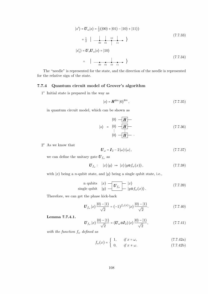
∣s′⟩ = UUUω ∣s⟩ = 12(∣00⟩ + ∣01⟩ − ∣10⟩ + ∣11⟩)
= 12 ∣ -r r r r
00 01
10
11
⟩
(7.7.33)
∣s′1⟩ = UUU sUUUω ∣s⟩ = ∣10⟩
= ∣ -r r r r00 01 10 11
⟩
(7.7.34)
The “needle” is represented for the state, and the direction of the needle is representedfor the relative sign of the state.
7.7.4 Quantum circuit model of Grover’s algorithm
1 Initial state is prepared in the way as
∣s⟩ =HHH⊗n ∣0⟩⊗n , (7.7.35)
in quantum circuit model, which can be shown as
∣s⟩ =
∣0⟩ HHH
∣0⟩ HHH⋮ ⋮
∣0⟩ HHH .
(7.7.36)
2 As we know thatUUUω = III2 − 2 ∣ω⟩ ⟨ω∣ , (7.7.37)
we can define the unitary gate UUUfω as
UUUfω ∶ ∣x⟩ ∣y⟩ ↦ ∣x⟩ ∣y⊕fω(x)⟩ , (7.7.38)
with ∣x⟩ being a n-qubit state, and ∣y⟩ being a single qubit state, i.e.,
n qubits ∣x⟩UUUfω
∣x⟩single qubit ∣y⟩ ∣y⊕fω(x)⟩ .
(7.7.39)
Therefore, we can get the phase kick-back
UUUfω ∣x⟩ ∣0⟩ − ∣1⟩√2
= (−1)fω(x) ∣x⟩ ∣0⟩ − ∣1⟩√2
. (7.7.40)
Lemma 7.7.4.1.
UUUfω ∣x⟩ ∣0⟩ − ∣1⟩√2
= (UUUω⊗III2) ∣x⟩∣0⟩ − ∣1⟩√
2, (7.7.41)
with the function fω defined as
fω(x) = 1, if x = ω, (7.7.42a)
0, if x ≠ ω. (7.7.42b)
108

This lemma can be represented in the form of Quantum Circuit diagram
∣0⟩1
HHH⊗n
UUUfω
∣0⟩2 UUUω ∣s⟩
⋮ ⋮ ⋮ ⋮
∣0⟩n∣0⟩−∣1⟩√
2
∣0⟩−∣1⟩√
2.
(7.7.43)
As we shall see that with ∣ω⟩ as an unknown state, UUUfω is actually an oracle.
Proof.
• In the case ∣x⟩ = ∣ω⟩.
UUUfω (∣ω⟩⊗ ∣0⟩ − ∣1⟩√2
) = (−1)f(ω)∣ω⟩⊗ ∣0⟩ − ∣1⟩√2
= −∣ω⟩⊗ ∣0⟩ − ∣1⟩√2
= UUUω ∣ω⟩⊗∣0⟩ − ∣1⟩√
2; (7.7.44)
• In the case ∣x⟩ ≠ ∣ω⟩.
UUUfω (∣x ≠ ω⟩⊗ ∣0⟩ − ∣1⟩√2
) = (−1)f(x≠ω)∣x ≠ ω⟩⊗ ∣0⟩ − ∣1⟩√2
= ∣x ≠ ω⟩⊗ ∣0⟩ − ∣1⟩√2
= UUUω ∣x ≠ ω⟩⊗∣0⟩ − ∣1⟩√
2. (7.7.45)
Note: How to perform Uω has to use of the black box Uf , which suggests thatperforming Uω takes the main part of the total performing time.
3 The second reflection operator
UUU s = 2 ∣s⟩ ⟨s∣ − III2, (7.7.46)
is at hand, because its realization does not involve the black-box and only includeselementary quantum gates. And we can derive that
UUU s = HHH⊗n (2 ∣0⟩⊗n ⟨0∣ − III⊗n2 )HHH⊗n
= HHH⊗nXXX⊗n (2 ∣1⟩⊗n ⟨1∣ − III⊗n2 )XXX⊗nHHH⊗n
= −HHH⊗nXXX⊗n (III⊗(n−1)2 ⊗HHH)θθθ(n) (III⊗(n−1)
2 ⊗HHH)XXX⊗nHHH⊗n, (7.7.47)
109
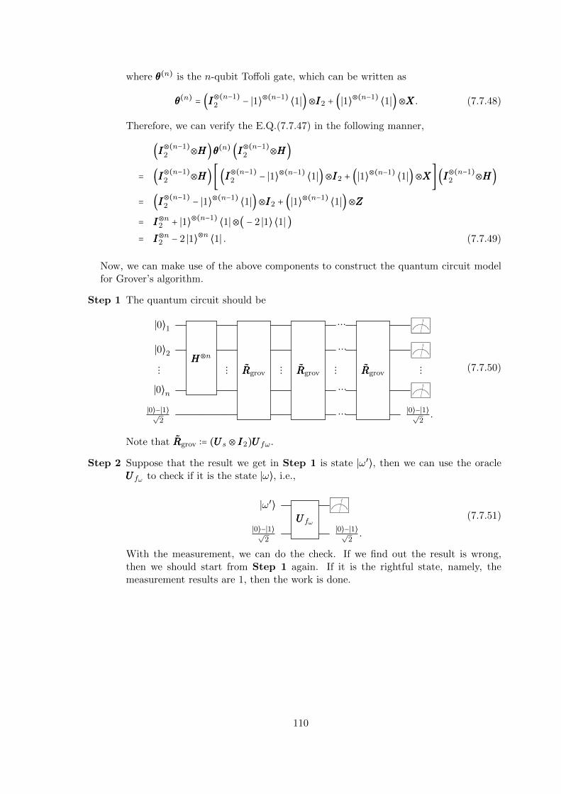
where θθθ(n) is the n-qubit Toffoli gate, which can be written as
θθθ(n) = (III⊗(n−1)2 − ∣1⟩⊗(n−1) ⟨1∣)⊗III2 + (∣1⟩⊗(n−1) ⟨1∣)⊗XXX. (7.7.48)
Therefore, we can verify the E.Q.(7.7.47) in the following manner,
(III⊗(n−1)2 ⊗HHH)θθθ(n) (III⊗(n−1)
2 ⊗HHH)
= (III⊗(n−1)2 ⊗HHH) [ (III⊗(n−1)
2 − ∣1⟩⊗(n−1) ⟨1∣)⊗III2 + (∣1⟩⊗(n−1) ⟨1∣)⊗XXX] (III⊗(n−1)2 ⊗HHH)
= (III⊗(n−1)2 − ∣1⟩⊗(n−1) ⟨1∣)⊗III2 + (∣1⟩⊗(n−1) ⟨1∣)⊗ZZZ
= III⊗n2 + ∣1⟩⊗(n−1) ⟨1∣⊗( − 2 ∣1⟩ ⟨1∣ )= III⊗n2 − 2 ∣1⟩⊗n ⟨1∣ . (7.7.49)
Now, we can make use of the above components to construct the quantum circuit modelfor Grover’s algorithm.
Step 1 The quantum circuit should be
∣0⟩1
HHH⊗n
RRRgrov RRRgrov
⋯
RRRgrov
LL ________
_ _ _ _ _ _ _ _
∣0⟩2⋯
LL ________
_ _ _ _ _ _ _ _
⋮ ⋮ ⋮ ⋮ ⋮
∣0⟩n ⋯LL ________
_ _ _ _ _ _ _ _
∣0⟩−∣1⟩√
2⋯ ∣0⟩−∣1⟩
√2.
(7.7.50)
Note that RRRgrov ∶= (UUU s ⊗ III2)UUUfω.
Step 2 Suppose that the result we get in Step 1 is state ∣ω′⟩, then we can use the oracleUUUfω to check if it is the state ∣ω⟩, i.e.,
∣ω′⟩UUUfω
LL ________
_ _ _ _ _ _ _ _
∣0⟩−∣1⟩√
2
∣0⟩−∣1⟩√
2.
(7.7.51)
With the measurement, we can do the check. If we find out the result is wrong,then we should start from Step 1 again. If it is the rightful state, namely, themeasurement results are 1, then the work is done.
110
Part III
Density Matrix and QuantumEntanglement
111

Chapter 8
Quantum Mechanics (II): DensityMatrix
References:
[Preskill] Chapter 2: Foundations I: states and ensembles;
[Nielsen & Chuang] Chapter 2: Introduction to quantum mechanics.
8.1 Density matrix as state of quantum open system
Density matrix (operator) describes the state of a quantum open system. It can be intro-duced in both physical and mathematical approaches. Usually, the quantum computer isan open subsystem, and with the environment by which suggests lots of noises, and theyform a closed system.
In the mathematical sense, we can view the projective measurement theory in termsof the density operator,
⟨ψ∣P n ∣ψ⟩ = ∑ak
⟨ψ∣P n ∣ak⟩ ⟨ak ∣ψ⟩
= ∑ak
⟨ak ∣ψ⟩ ⟨ψ∣P n ∣ak⟩
= tr(∣ψ⟩ ⟨ψ∣P n)= tr(ρPn), (8.1.1)
with the density operator defined as
ρ ∶= ∣ψ⟩ ⟨ψ∣ , (8.1.2)
and all ∣ak⟩ ∈ ∣aj⟩ ∣A ∣aj⟩ = aj ∣aj⟩ , ∣aj⟩ ∈H being normalized. Therefore,
⟨A⟩ = ⟨ψ ∣A ∣ψ⟩= ∑
n
an ⟨ψ ∣P n ∣ψ⟩
= ∑n
antr(ρP n)
= tr(ρA). (8.1.3)
We can claim that the probability to obtain the outcome an when measuring A is actually
Prob(an) = tr(ρP n). (8.1.4)
112

In the physical sense, for the quantum closed system with the initial state ∣ψ⟩,
∣ψ⟩ =∑n
cn ∣n⟩ ,
where ∣n⟩ is an orthonormal basis for the Hilbert space H . The probability to get thepost-measurement states ∣n⟩ is
Prob(∣n⟩) = ∣ ⟨n ∣ψ⟩ ∣2
∣ ⟨ψ ∣ψ⟩ ∣2. (8.1.5)
Question: What is the post-measurement state of an open system?
ρ ∶=∑n
pn ∣n⟩ ⟨n∣ , with ∑n
pn = 1 and pn ≥ 0. (8.1.6)
The ρ is the so-called density matrix, which will be defined later. And the density operatorρ is equivalent to state ensemble ∣n⟩ , pn, in the Quantum Mechanical sense.
Remark. In the description of the density matrix, the ambiguity of the global phasefactor with non-physical meaning is removed,
∣ψ⟩ ≅ eiα∣ψ⟩, (8.1.7)
ρ = ∣ψ⟩⟨ψ∣, ρα = eiα∣ψ⟩⟨ψ∣e−iα = ρ. (8.1.8)
8.1.1 State ensemble formalism of density matrix
Def 8.1.1. The state ensemble is a set of state ∣ψi⟩ each attached with a probability pi,namely
∣ψi⟩ , pi ∣ i = 1, . . ., n, with pi ∈ [0,1] andn
∑i=1
pi = 1. (8.1.9)
It means that the physical system has the probability of pi to be prepared in the state ∣ψi⟩.
For any observable A, the expectation value of A is
⟨A⟩ =n
∑i=1
pi ⟨ψi∣A ∣ψi⟩
=dim H
∑k=1
n
∑i=1
pi ⟨ψi ∣k⟩ ⟨k ∣A ∣ψi⟩
=dim H
∑k=1
n
∑i=1
⟨k∣A ∣ψi⟩pi ⟨ψi ∣k⟩
=dim H
∑k=1
⟨k∣An
∑i=1
( ∣ψi⟩pi ⟨ψi∣ ) ∣k⟩
=dim H
∑k=1
⟨k∣Aρ ∣k⟩
= tr(Aρ),
with ρ = ∑ni=1 pi ∣ψi⟩ ⟨ψi∣,
⟨A⟩ =n
∑i=1
pi ⟨ψi∣A ∣ψi⟩ = tr(Aρ), (8.1.10)
where ∣k⟩ ∣ k = 1, . . .,dimH is an orthonormal basis for the Hilbert space H .
113

Def 8.1.2. The density matrix for the system described by the state ensemble, as shownin E.Q. (8.1.9), is defined as
ρ ∶=n
∑i=1
pi ∣ψi⟩ ⟨ψi∣ , (8.1.11)
• if n = 1, this represents a pure state, and the system is completely specified;
• if n ≥ 2, this represents a mixed state, and the system is partially specified.
Thm 8.1.1.1. A sufficient and necessary condition to tell whether the density operator ρrepresents a pure state or a mixed state is
pure state ⇐⇒ ρ2 = ρ, trρ2 = 1;mixed state ⇐⇒ ρ2≠ρ, trρ2 < 1.
(8.1.12)
Proof. As we shall show later that the density operators are non-negative and self-adjointwith unit trace. It is always possible to use a set of orthonormal eigenvectors of the densityoperator ρ as the basis to expand the whole Hilbert space H . In that way, the densitymatrix ρ is diagonalized, with its eigenvalues λi lying along the diagonal position of thematrix:
ρ =dim H
∑i=1
λi ∣λi⟩ ⟨λi∣ . (8.1.13)
There we can also get ρ:
ρ2 =dim H
∑i,j=1
λiλj ∣λi⟩ ⟨λi ∣λj⟩ ⟨λj ∣
=dim H
∑i,j=1
λiλj ∣λi⟩ ⟨λj ∣ δij
=dim H
∑i=1
λ2i ∣λi⟩ ⟨λi∣ . (8.1.14)
trρ2 =dim H
∑i=1
λ2i ≤ (
dim H
∑i=1
λi)2
= 1. (8.1.15)
Therefore, the sufficient and necessary condition that ρ is equal to ρ2 should be
λi = λ2i , with i = 1, . . .,dimH . (8.1.16)
With ρ being self-adjoint and non-negative with unit trace, namely
dim H
∑i=1
λi = 1, with λi ∈ R and λi ≥ 0, i = 1, . . .,dimH , (8.1.17)
it then can be inferred that E.Q. (8.1.16) is equivalent to that there should be only one λjbeing 1 while all other λi with i ≠ j are vanishing. And it also says that the same thing asE.Q. (8.1.12), since with only one eigenvalue for the density operator, it is sufficient andnecessary to get the pure state.
Thm 8.1.1.2. The density operator ρ should be subject to the following time-evolutionequation
ih∂
∂tρ(t) = [H,ρ(t)]. (8.1.18)
114

Notice: We can see that E.Q. (8.1.18) is very similar to the Heisenberg equation, but it’snot a Heisenberg equation at all.This can be shown in the following way.
Proof. To get the time evolution of the physical system, we may start from the stateensemble as given in E.Q. (8.1.9). Every state vector ∣ψi⟩ within the state ensembleshould follow the Shrodinger equation
ih∂
∂t∣ψi(t)⟩ =H ∣ψi(t⟩ ,
or we can get the state ensemble at time t
∣ψi(t)⟩ , pi ∣ i = 1, . . ., n, (8.1.19)
with∣ψi(t)⟩ ∶=UUU (t) ∣ψi⟩ , (8.1.20)
where UUU (t) is defined in E.Q. (2.1.17). Therefore, the density operator at time t shouldbe
ρ(t) =n
∑i=1
pi ∣ψi(t)⟩ ⟨ψi(t)∣ . (8.1.21)
Now, we can derive the time-evolution equation for ρ:
ih∂
∂tρ(t) =
n
∑i=1
pi(ih∂
∂t∣ψi(t)⟩ ⟨ψi(t)∣ + ∣ψi(t)⟩ ih
∂
∂t⟨ψi(t)∣ )
=n
∑i=1
pi(H ∣ψi(t)⟩ ⟨ψi(t)∣ + ∣ψi(t)⟩ ⟨ψi(t)∣ (−H))
= [ρ,H]
which is equivalent to E.Q. (8.1.18).
8.1.2 Operator formalism of density matrix
Now, we come to discuss the properties of the density matrix.
Def 8.1.3. The density matrix ρ is a non-negative self-adjoint operator with unit trace,i.e.,
⎧⎪⎪⎪⎨⎪⎪⎪⎩
ρ† = ρ self-adjoint operator,ρ ≥ 0 non-negative,
trρ = 1 unit trace.(8.1.22)
Notice: ρ being non-negative means that all its eigenvalues are non-negative, which isalso equivalent to that given any state its expectation value should be non-negative.
Thm 8.1.2.1. The operator formalism of the density matrix ρ is equivalent to its stateensemble description.
Proof. To derive the three properties of the density operator ρ, we may start from thedefinition (8.1.11), for it not only represents the mixed state case, but also the pure statecase.
115
• Self-adjoint
ρ† = (n
∑i=1
pi ∣ψi⟩ ⟨ψi∣)†
(8.1.23)
=n
∑i=1
p∗i ∣ψi⟩ ⟨ψi∣ (8.1.24)
=n
∑i=1
pi ∣ψi⟩ ⟨ψi∣ (8.1.25)
= ρ, (8.1.26)
since pi ∈ R for i = 1, . . ., n.
• Non-negative
⟨φ ∣ρ ∣φ⟩ =n
∑i=1
pi ⟨φ ∣ψi⟩ ⟨ψi ∣φ⟩
=n
∑i=1
pi∣ ⟨ψi ∣φ⟩ ∣2, (8.1.27)
where ∣φ⟩ is an arbitrary vector in Hilbert space H . Given pi ≥ 0 for all i = 1, . . ., n,it’s obvious that ⟨φ ∣ρ ∣φ⟩ is non-negative, namely ρ is non-negative.
• Unit trace
trρ = tr(n
∑i=1
pi ∣ψi⟩ ⟨ψi∣) (8.1.28)
=n
∑i=1
pitr (∣ψi⟩ ⟨ψi∣) (8.1.29)
=n
∑i=1
pi (8.1.30)
= 1, (8.1.31)
because pi with i = 1, . . ., n would add up to 1 and all ∣ψi⟩ are assumed to be nor-malized.
8.1.3 Reduced density matrix (State for subsystem)
Let’s assume that the state of the composite physical system C consisted of subsystem Aand subsystem B, is in state ∣ψ⟩C. Then, we can get the density matrix for the compositephysical system C,
ρAB = ∣ψ⟩AB ⟨ψ∣ . (8.1.32)
That represents a pure state, as we consider the composite physical system as a whole.But, now we examine only the subsystem A (Alice) of the composite system. We can getthe observable MA for the subsystem of Alice, expressed in Hilbert space HAB of thecomposite system C as
MA⊗IB.
Therefore, the expectation value of the observable MA is then
⟨MA⟩ = AB ⟨ψ∣MA⊗IB ∣ψ⟩AB
= tr((MA⊗IB)ρAB)
= trA(MAρA), (8.1.33)
116
whereρA = trBρAB. (8.1.34)
And we have used the facts that
trOAB = trA (trBOAB) ,
tr (MAOAB) = trA (MAtrBOAB) ,(8.1.35)
which can be proved simply by expressing all the operators in the form of kets and bras.The reduced density matrix ρρρA can describe the subsystem A, given the density opera-
tor of the compound physical system is ρρρAB, in the following sense. IfOOOA is an operator cor-responding to an arbitrary observable defined in the subsystem A, namely OOOA ∈ B(HA),then we can express it in the total Hilbert space HAB ∶=HA⊗HB as
OOOA⊗IIIB. (8.1.36)
Therefore, the expectation value of the observable OOOA should be
⟨OOOA⟩ = trAB(OOOAρρρAB)= trA[trB(OOOAρρρAB)]= trA(OOOAtrBρρρAB)= trA(OOOAρρρA). (8.1.37)
On the other hand, it really makes a density operator because
• self-adjoint:
ρρρ†A = (trBρρρAB)†
= trBρρρ†AB
= trBρρρAB
= ρρρA; (8.1.38)
• unit trace:
trAρρρA = trA (trBρρρAB)= trABρρρAB
= 1; (8.1.39)
• nonnegative:
A ⟨ψ ∣ρρρA ∣ψ⟩A = trA (ρρρA ∣ψ⟩A ⟨ψ∣)= trAB [ρρρAB(∣ψ⟩A ⟨ψ∣⊗IIIB)]
namely
A ⟨ψ ∣ρρρA ∣ψ⟩A ≥ 0, ∀∣ψ⟩A ∈ HA (8.1.40)
since the probability for the compound system ρρρAB found in state ∣ψ⟩A ⟨ψ∣⊗IIIB shouldbe nonnegative.
E.g. Reduced density matrix ρρρA of the general bipartite system
∣ψ⟩AB =∑i∑µ
aiµ∣i⟩A ⊗ ∣µ⟩B, (8.1.41)
ρρρA = trBρρρAB ≡∑µ
⟨µ∣ρAB ∣µ⟩B =∑µ∑i∑j
aiµa∗iµ∣i⟩A⟨j∣, (8.1.42)
where the partial tracetrB (∣µ⟩B⟨ν∣) = ⟨ν∣µ⟩B = δµν . (8.1.43)
117

8.2 Mixed state formalism of a qubit
Thm 8.2.0.1. Density matrix in the two-dimension Hilbert space H2, can be representedas
ρρρ(p) ∶= 1
2(III2 + p⋅σσσ), (8.2.1)
with p ∈ R3 satisfying ∥p∥ ≤ 1. And we give the vector p the name of the “polarizationvector”.
Proof. Firstly, we would prove that any density matrix in the two-dimensional Hilbertspace H2 can be expressed in the form as E.Q. (8.2.1). Secondly, we would show thatwith the constraint ∥p∥ ≤ 1, E.Q. (8.2.1) is a density matrix.
a) Any density matrix in the 2-dimensional Hilbert space H2 can be represented in theform of E.Q. (8.2.1).The most general 2-dimensional matrix would have the form
ρρρ = (a bc d
) , (8.2.2)
which has 2×4 = 8 degrees of freedom. But to make a density matrix for a physicalsystem, the matrix ρ must satisfy three constraints.
(i) Self-adjoint: A density matrix must be self-adjoint, i.e., ρρρ† = ρρρ, whichmeans
(a∗ c∗
b∗ d∗) = (a b
c d) ⇐⇒
⎧⎪⎪⎪⎪⎪⎪⎪⎨⎪⎪⎪⎪⎪⎪⎪⎩
a∗ = ad∗ = db∗ = cc∗ = b
, (8.2.3)
which actually makes four constraints for ρ, that would reduce the degrees offreedom from eight to four.
(ii) Unit trace: The trace of a density matrix must be equal to one, i.e.,
trρρρ = 1 ⇐⇒ a + d = 1, (8.2.4)
which makes a fifth constraint to ρρρ. The degrees of freedom has come down tothree now.
(iii) Positive: The density matrix must have all its eigenvalues to be non-negative.This would appear as inequalities, namely “holonomic constraints” in the lan-guage of Classical Mechanics, which would never reduce a freedom but couldabsolutely set some kind of range for the parameters.
On the other hand, we know that, the density matrices for the Hilbert space H2
can actually be viewed as a vector space B(H2). The three Pauli matrices plusthe identity matrix can be the vector basis for B(H2), because they are linearlyindependent to each other. Therefore, it would be clear that any density matrix canbe expressed in the form of E.Q. (8.2.1).
118

b) Now, we set to prove that iff ∥p∥ ≤ 1, E.Q.(8.2.1) would be a density matrix. FromE.Q.(8.2.1) we get
ρρρ = 1
2( 1 + p3 p1 − ip2
p1 + ip2 1 − p3) with p1, p2, p3 ∈ R. (8.2.5)
This definition implies apparently that ρρρ is self-adjoint. And we can immediatelyget the trace and the determinant of ρρρ:
trρρρ = 1
2((1 + p3) + (1 − p3)) = 1, (8.2.6)
detρρρ = 1
4[(1 + p3)(1 − p3) − (p1 − ip2)(p1 + ip2)] =
1
4(1 − ∥p∥2). (8.2.7)
Let’s denote the two eigenvalues of ρρρ with λ1 and λ2, then
⎧⎪⎪⎨⎪⎪⎩
trρρρ = λ1 + λ2 = 1,
detρρρ = λ1λ2 = 14(1 − ∥p∥2),
from which we can infer that ρρρ being nonnegative is equivalent to
λ1 ≥ 0λ2 ≥ 0
⇐⇒ ∥p∥ ≤ 1. (8.2.8)
Therefore, ρρρ defined in E.Q. (8.2.1) is a density matrix iff ∥p∥ ≤ 1.
c) We can now claim that, any density operator for two-level system attached withHilbert space H2, can be written as E.Q. (8.2.1).
8.2.1 Why polarization vector?
We firstly calculate the expectation value ⟨σσσ⋅n⟩, given the physical system is in the statedescribed by the density operator ρρρ defined in E.Q. (8.2.1),
⟨σσσ⋅n⟩ = tr[(σσσ⋅n)ρρρ]
= tr [1
2(σσσ⋅n)(1 + p⋅σσσ)]
= 1
2tr(σσσ⋅n) + tr[(σσσ⋅n)(p⋅σσσ)]. (8.2.9)
Amid, we can get
tr(σσσ⋅n) = tr(n1σσσ1 + n2σσσ2 + n3σσσ3)= n1trσσσ1 + n2trσσσ2 + n3trσσσ3
= 0, (8.2.10)
where we have used the fact that
trσσσi = 0, with i = 1,2,3. (8.2.11)
119

And, we can also get
tr[(σσσ⋅n)(p⋅σσσ)] = tr⎛⎝
3
∑i,j=1
nipjσiσj⎞⎠
=3
∑i,j=1
nipjtr(σσσiσσσj)
= 23
∑i,j=1
nipjδij
= 2n⋅p. (8.2.12)
In the above derivation we have used the relation
tr(σσσiσσσj) = 2δij , (8.2.13)
which can be derived in the following manner
trσσσ2i = trIII2 = 2
i≠j ∶ tr(σσσiσσσj) = tr(i∑3k=1 εijkσσσk) = i∑
3k=1 εijktrσσσk = 0
⇒ tr(σσσiσσσj) = 2δij , i, j = 1,2,3.
Now, by substituting E.Q. (8.2.10) and E.Q. (8.2.12) into E.Q. (8.2.9), we can concludethat
⟨σσσ⋅n⟩ = n⋅p,
which is equivalent to
Thm 8.2.1.1.tr((σσσ⋅n)ρρρ(p)) = n⋅p, (8.2.14)
with n, p ∈ R3 and ∥n∥ = 1.
With this theorem, we can understand why we call p the “polarization vector”:
(i) ⟨σσσ⋅n⟩ = tr((σσσ⋅n)ρρρ(p)) = 0, for p n;
(ii) ⟨σσσ⋅n⟩ = tr((σσσ⋅n)ρρρ(p)) = 1, for p = n;
(iii) ⟨σσσ⋅n⟩ = tr((σσσ⋅n)ρρρ(p)) = −1, for p = −n;
(iv) ⟨σσσ⋅n⟩ = tr((σσσ⋅n)ρρρ(p)) = 0, for p = 0, ∀n ∈ R3.
We can see that p = 0 implies no polarization orientation, which shows “no information”.
8.2.2 Pure state and mixed state in two-dimensional Hilbert space H2
Thm 8.2.2.1. If the state in the two-dimensional Hilber space H2, which means that thestate has the density matrix defined in E.Q. (8.2.1). Then the state of the physical systemis
a pure state, if p is on the Bloch sphere, ∥p∥ = 1,a mixed state, if p is inside the Bloch sphere, ∥p∥ < 1.
120

We can show that
ρρρ2(p) = 1
4(1 + 2p⋅σσσ + (p⋅σσσ)2) = 1
4(1 + 2p⋅σσσ + p2), (8.2.15)
because
(p⋅σσσ)2 =3
∑i=1
p2iσσσ
2i +
3
∑i,j=1i>j
pipjσσσi,σσσj
=3
∑i=1
p2i + 0
= ∥p∥2. (8.2.16)
Therefore,
ρρρ2(p) = ρρρ(p), if p is on the Bloch sphere, ∥p∥ = 1;ρρρ2(p) ≠ ρρρ(p), if p is inside the Bloch sphere, ∥p∥ < 1.
(8.2.17)
Thus ρρρ2(p) ≠ ρρρ(p) or ∥p∥ < 1 is sufficient to claim that ρρρ(p) is a mixed state. On the otherhand, we can get some examples of case ∥p∥ = 1:
• p = ez, ρρρ(ez) = (1 00 0
) = ∣0⟩ ⟨0∣ = ∣↑z⟩ ⟨↑z ∣;
• p = ex, ρρρ(ex) = 12 (1 1
1 1) = 1
2( ∣0⟩ + ∣1⟩ )( ⟨0∣ + ⟨1∣ ) = ∣+⟩ ⟨+∣ = ∣↑x⟩ ⟨↑x∣ ;
• p = ey, ρρρ(ey) = 12 (1 −ii 1
) = 12( ∣0⟩ + i ∣1⟩ )( ⟨0∣ − i ⟨1∣ ) = ∣↑y⟩ ⟨↑y ∣ .
In general, if ∥p∥ = 1, we can express p as p = (sin θ cosϕ, sin θ sinϕ, cos θ),
ρρρ(p) = 1
2( 1 + cos θ sin θ cosϕ − i sin θ sinϕ
sin θ cosϕ + i sin θ sinϕ 1 − cos θ)
= 1
2(1 + cos θ sin θe−iϕ
sin θeiϕ 1 − cos θ)
=⎛⎝
cos2 θ2 sin θ
2 cos θ2e−iϕ
sin θ2 cos θ2e
iϕ sin2 θ2
⎞⎠
= ( cos θ2sin θ
2eiϕ)(cos θ2 sin θ
2e−iϕ)
= ∣ψ+(θ,ϕ)⟩ ⟨ψ+(θ,ϕ)∣= ∣↑p⟩ ⟨↑p∣ . (8.2.18)
Therefore, ∥p∥ = 1 is a sufficient condition for that ρρρ(p) is a pure state.Given that any state for a two-level physical system, such as spin-1/2 systems, which canbe described by ρρρ(p) as defined in E.Q. (8.2.1), we can conclude that now:
• ∥p∥ = 1 is a sufficient and necessary condition for that ρρρ(p) is a pure state;
• ∥p∥ < 1 is a sufficient and necessary condition for that ρρρ(p) is a mixed state.
121
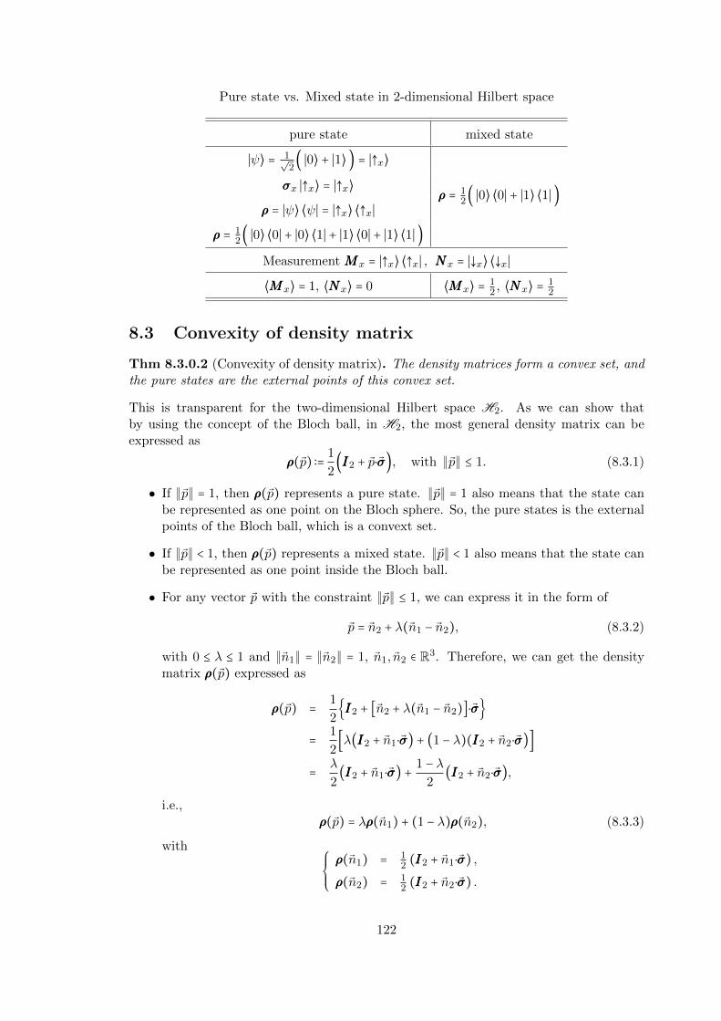
Pure state vs. Mixed state in 2-dimensional Hilbert space
pure state mixed state
∣ψ⟩ = 1√2( ∣0⟩ + ∣1⟩ ) = ∣↑x⟩
ρρρ = 12( ∣0⟩ ⟨0∣ + ∣1⟩ ⟨1∣ )
σσσx ∣↑x⟩ = ∣↑x⟩
ρρρ = ∣ψ⟩ ⟨ψ∣ = ∣↑x⟩ ⟨↑x∣
ρρρ = 12( ∣0⟩ ⟨0∣ + ∣0⟩ ⟨1∣ + ∣1⟩ ⟨0∣ + ∣1⟩ ⟨1∣ )
Measurement MMMx = ∣↑x⟩ ⟨↑x∣ , NNNx = ∣↓x⟩ ⟨↓x∣
⟨MMMx⟩ = 1, ⟨NNNx⟩ = 0 ⟨MMMx⟩ = 12 , ⟨NNNx⟩ = 1
2
8.3 Convexity of density matrix
Thm 8.3.0.2 (Convexity of density matrix). The density matrices form a convex set, andthe pure states are the external points of this convex set.
This is transparent for the two-dimensional Hilbert space H2. As we can show thatby using the concept of the Bloch ball, in H2, the most general density matrix can beexpressed as
ρρρ(p) ∶= 1
2(III2 + p⋅σσσ), with ∥p∥ ≤ 1. (8.3.1)
• If ∥p∥ = 1, then ρρρ(p) represents a pure state. ∥p∥ = 1 also means that the state canbe represented as one point on the Bloch sphere. So, the pure states is the externalpoints of the Bloch ball, which is a convext set.
• If ∥p∥ < 1, then ρρρ(p) represents a mixed state. ∥p∥ < 1 also means that the state canbe represented as one point inside the Bloch ball.
• For any vector p with the constraint ∥p∥ ≤ 1, we can express it in the form of
p = n2 + λ(n1 − n2), (8.3.2)
with 0 ≤ λ ≤ 1 and ∥n1∥ = ∥n2∥ = 1, n1, n2 ∈ R3. Therefore, we can get the densitymatrix ρρρ(p) expressed as
ρρρ(p) = 1
2III2 + [n2 + λ(n1 − n2)]⋅σσσ
= 1
2[λ(III2 + n1⋅σσσ) + (1 − λ)(III2 + n2⋅σσσ)]
= λ
2(III2 + n1⋅σσσ) +
1 − λ2
(III2 + n2⋅σσσ),
i.e.,ρρρ(p) = λρρρ(n1) + (1 − λ)ρρρ(n2), (8.3.3)
with ⎧⎪⎪⎨⎪⎪⎩
ρρρ(n1) = 12 (III2 + n1⋅σσσ) ,
ρρρ(n2) = 12 (III2 + n2⋅σσσ) .
122

Therefore, we can also get
ρρρ(p)⇐⇒ λ, ∣ψ+(n1)⟩ ; (1 − λ), ∣ψ+(n2)⟩ . (8.3.4)
Remark: The same mixed state density matrix may have different interpretations of stateensembles. We can make an easy example to demonstrate this, for instance
ρ ∶= 1
2I. (8.3.5)
The density matrix defined in this form can be interpreted as state ensemble consistedof an arbitrary orthonormal basis vector set for the Hilbert space H , with each statevector attached with the probability 1/dimH .
Question: Why can the same mixed state density matrices have different interpretationsof state ensembles?Information encoded in the density matrix of the mixed state (which may denotethe subsystem of the entangled pure state), can only be partially specified. Andthe entanglement information (as partial information of the composite system) cannot be reveled in the subsystem individually, which leads to the ambiguity of theinterpretation of state ensembles. As we could see, the state is more entangling, theinformation is more hidden.
8.4 Two-qubit system and its subsystem
Two-qubit system and its subsystem
entire system subsystem
two-qubit ∈H2⊗H2 one-qubit ∈H2
density matrix reduced density matrix
pure state (maybe) mixed state
(exactly known) (partially known or completely unkonwn)
8.4.1 Example: EPR pair (Bell state)
We consider a state of the composite physical system, which is made up of two subsystemsA (Alice) and B (Bob),
∣ψ⟩AB ∶= 1√2( ∣00⟩ + ∣11⟩ )
AB= 1√
2( ∣0⟩A⊗ ∣0⟩B + ∣1⟩A⊗ ∣1⟩B ). (8.4.1)
And the corresponding density matrix should be
ρρρAB ∶= ∣ψ⟩AB ⟨ψ∣ = 1
2( ∣00⟩AB ⟨00∣ + ∣00⟩AB ⟨11∣ + ∣11⟩AB ⟨00∣ + ∣11⟩AB ⟨11∣ ). (8.4.2)
We can check that ρρρ2AB = ρρρAB,
ρρρ2AB = ∣ψ⟩AB ⟨ψ ∣ψ⟩AB ⟨ψ∣ = ∣ψ⟩AB ⟨ψ∣ = ρρρAB, (8.4.3)
123

amid we have use the fact that
AB ⟨ψ ∣ψ⟩AB = 1
2(A ⟨0∣⊗B ⟨0∣ + A ⟨1∣A⊗B ⟨1∣ )( ∣0⟩A⊗ ∣0⟩B + ∣1⟩A⊗ ∣1⟩B )
= 1
2(A ⟨0 ∣0⟩A B ⟨0 ∣0⟩B + A ⟨0 ∣1⟩A B ⟨0 ∣1⟩B
+ A ⟨1 ∣0⟩A B ⟨1 ∣0⟩B + A ⟨1 ∣1⟩A B ⟨1 ∣1⟩B )
= 1
2(1 + 0 + 0 + 1)
= 1.
Therefore, the entire physical system is in pure state.Now, we consider the reduced density matrix for the subsystem A (Alice), which is aone-qubit system,
ρρρA ∶= trBρρρAB. (8.4.4)
From above definition, we can get
ρρρA =1
∑i=0
B ⟨i∣ρρρAB ∣i⟩B
= 1
2( ∣0⟩A ⟨0∣ + ∣1⟩A ⟨1∣ )
= 1
2III2. (8.4.5)
For an arbitrary orientation, n = (sin θ cosϕ, sin θ sinϕ, cos θ),
⟨n⋅σσσA⟩ = trA[(n⋅σσσA)ρρρA]
= 1
2trA(n⋅σσσA)
= 0. (8.4.6)
Therefore, in this case the polarization vector for the subsystem A should be a null vectorin R3, and we can extract “no information” from this subsystem.Remark: Generally, the composite system with pure state, is exactly known. While, forthe the subsystem, which is usually in mixed state, is often partially known or nothingknown.
Def 8.4.1 (Maximally entanglement). If a bipartite ρρρAB is a pure state with ρρρA = 12IIIA,
then ρρρAB is called maximally entangled.
8.4.2 Maximally entangled two-qubit pure states
Thm 8.4.2.1. All Bell states are maximally entangled.
Proof. This is transparent from E.Q. (3.3.11),
∣ψ(i, j)⟩AB = 1√2[∣0i⟩AB + (−1)j ∣1i⟩AB]
124

that
ρρρA = trB ∣ψ(i, j)⟩AB ⟨ψ(i, j)∣= B ⟨i ∣ψ(i, j)⟩AB ⟨ψ(i, j)∣ i⟩B + B ⟨i ∣ψ(i, j)⟩AB ⟨ψ(i, j)∣ i⟩B
= 1
2∣0⟩A ⟨0∣ + 1
2∣1⟩A ⟨1∣
= 1
2IIIA, (8.4.7)
and
ρρρB = trA ∣ψ(i, j)⟩AB ⟨ψ(i, j)∣= B ⟨0 ∣ψ(i, j)⟩AB ⟨ψ(i, j)∣0⟩B + B ⟨1 ∣ψ(i, j)⟩AB ⟨ψ(i, j)∣1⟩B
= 1
2∣i⟩A ⟨i∣ + 1
2∣⟨i∣⟩A ⟨i∣
= 1
2IIIB. (8.4.8)
Therefore, we can conclude now that every Bell state ∣ψ(i, j)⟩ is maximally entangled.
Remark:
(1) Local unitary transformations, e.g. III2⊗XXXiZZZj , preserve the entangling property;
(2) With ρρρA = ρρρB = 12III2, we cannot acquire any information from local measurement on
any one of the two subsystems.
(3) For product pure state, there is no entanglement. For example,
∣φ⟩AB = ∣n⟩A⊗ ∣m⟩B ,
has the corresponding reduced density matrices
ρρρA = ∣n⟩A ⟨n∣ ,ρρρB = ∣m⟩B ⟨m∣ ,
with ∣n∣ = ∣m∣ = 1. There is no information can be hidden in the subsystem in thiscase. We may say that the more entangled a state is, the more hidden of the quantuminformation is.
8.4.3 Monogamy of maximal entanglement
Alice and Bob share a maximal entangled state (e.g. the Bell state ∣φ+⟩). And here comesa third party, Eve. Eve wants to destroy the state shared by Alice and Bob, i.e., destroy∣φ+⟩.
∣φ+⟩AB⊗∣0⟩E´¹¹¹¹¹¹¹¹¹¹¹¹¹¹¹¹¹¹¹¹¹¹¹¹¹¹¹¹¸¹¹¹¹¹¹¹¹¹¹¹¹¹¹¹¹¹¹¹¹¹¹¹¹¹¹¹¹¶
separable
↓∣ψ⟩ABE´¹¹¹¹¹¹¹¹¸¹¹¹¹¹¹¹¹¶entangled
= ∣00⟩AB∣e00⟩E + ∣01⟩AB∣e01⟩E
+∣10⟩AB∣e10⟩E + ∣11⟩AB∣e11⟩E. (8.4.9)
But, Alice and Bob can avoid it by Bell measurements XA⊗XB and ZA⊗ZB and inform-ing each other their measurements results.
125

• After measuring ZA⊗ZB, they get the result of 1, then
∣ψ⟩ABE´¹¹¹¹¹¹¹¹¸¹¹¹¹¹¹¹¹¶entangled
↓∣ψ′⟩
ABE´¹¹¹¹¹¹¹¹¹¹¸¹¹¹¹¹¹¹¹¹¹¹¶entangled
= ∣00⟩AB∣e00⟩E + ∣11⟩AB∣e11⟩E (8.4.10)
• After measurement of XA⊗XB, the result is 1, then the final state has to be
∣ψ′⟩ABE
´¹¹¹¹¹¹¹¹¹¹¸¹¹¹¹¹¹¹¹¹¹¹¶entangled
↓
∣ψ′′⟩ABE
´¹¹¹¹¹¹¹¹¹¹¹¹¹¹¸¹¹¹¹¹¹¹¹¹¹¹¹¹¹¶separable
= 1√2(∣00⟩AB + ∣11⟩AB)⊗ ∣e⟩E . (8.4.11)
in which the state of Eve ∣e⟩E has been decoupled with ∣φ+⟩AB.
126

Chapter 9
Schmidt Decomposition,Purification and GHJW Theorem
References:
[Preskill] Chapter 2: Foundations I: states and ensembles;
[Nielsen & Chuang] Chapter 2: Introduction to quantum mechanics.
9.1 Introduction
Let’s consider a bipartite composite system with two subsystems A (Alice) and B(Bob), interacting with each other. The state of the composite system can be describedby the pure state ∣ψ⟩AB with the corresponding density matrix ρρρAB = ∣ψ⟩AB ⟨ψ∣. Andthe density matrix of the subsystem A should be ρρρA = trBρρρAB = trA( ∣ψ⟩AB ⟨ψ∣ ). Beforefurther talking about the measurement and quantum operation on the subsystem of thecomposite system, in this chapter, we would introduce some relations between subsystemand composite system. And Figure 9.1 illustrates the plan for this chapter.
Schmidt decomposition
Quantum entanglement Purification
GHJW theorem
Figure 9.1: Plan for chapter 14.
9.2 Schmidt decomposition and quantum entanglement
9.2.1 Schmidt decomposition
Thm 9.2.1.1 (Schmidt decomposition). In a bipartite system HA⊗HB, a bipartite purestate ∣ψ⟩AB can be expressed in the form of
∣ψ⟩AB =∑i
√pi ∣i⟩A⊗ ∣i′⟩
B, with pi ≥ 0, ∑
i
pi = 1, (9.2.1)
127

where ∣i⟩A and ∣i′⟩B are orthonormal basis for HA and HB respectively. This is theso-called Schmidt decomposition.
Example: Bell state (EPR state)
∣ψ⟩AB = 1√2( ∣00⟩ + ∣11⟩ )
AB
= 1√2
1
∑i=0
∣ii⟩AB
= 1√2
1
∑i=0
∣i⟩A⊗ ∣i⟩B , (9.2.2)
with√p0 =
√p1 = 1√
2. We can also get
⎧⎪⎪⎨⎪⎪⎩
ρρρA = 12IIIA,
ρρρB = 12IIIB.
(9.2.3)
Remark: For ∣ψ⟩AB = ∑i√pi ∣i⟩A⊗ ∣i′⟩B, we may have dimHA≠dimHB. But ρρρA and ρρρB
would have the same diagonalized formalism, i.e.,
ρρρA =∑i
pi ∣i⟩A ⟨i∣ , ρρρB =∑i
pi ∣i′⟩B⟨i′∣ . (9.2.4)
Def 9.2.1. Schmidt coefficient and Schmidt number:
1. The non-vanishing pi in E.Q. (9.2.1) are called Schmidt coefficients.
2. The number of Schmidt coefficients is called Schmidt number.
9.2.2 Quantum entanglement
Def 9.2.2. Separable and Entangled bipartite pure states:
• if the Schmidt number is 1, ∣ψ⟩AB is called separable, which means that the statevector of the composite physical system can be expressed as
∣ψ⟩AB = ∣φ⟩A⊗ ∣χ⟩B , (9.2.5)
which is the so-called product state;
• if the Schmidt number is greater than 1, then the state ∣ψ⟩AB is called entangledstate;
• if the reduced density matrices for the subsystems are all identity matrices, namely
⎧⎪⎪⎨⎪⎪⎩
ρρρA = 12IIIA,
ρρρB = 12IIIB,
(9.2.6)
then ∣ψ⟩AB is called maximally entangled. (We have actually mentioned this at theend of the last chapter (Ref. page 124).)
Note: We would discuss about the entanglement definition for bipartite mixed state andmultipartite mixed state later.
128

9.2.3 Proof for the theorem of the Schmidt decomposition
Proof. The key point to get the Schmidt decomposition of an arbitrary state ∣ψ⟩AB definedas
∣ψ⟩AB ∶=∑i,µ
biµ ∣i⟩A⊗ ∣µ⟩B , (9.2.7)
with ∣i⟩A and ∣µ⟩B being orthonormal basis for HA and HB respectively, is to get boththe reduced density matrices ρρρA and ρρρB diagonalized. And therefore the correspondingdensity matrix of the composite physical system should be
ρρρAB ∶= ∣ψ⟩AB ⟨ψ∣ = ∑i,j,µ,ν
biµb∗jν ∣i⟩A ⟨j∣⊗ ∣µ⟩B ⟨ν∣ . (9.2.8)
Now, we can go on step by step.
Step 1:Compute ρρρA by the taking the partial trace of ρρρAB over HB:
ρρρA = trBρρρAB
= ∑µ′
B ⟨µ′∣ρρρAB ∣µ′⟩B
= ∑i,µ,j,ν,µ′
biµb∗jν( ∣i⟩A ⟨j∣ )⊗( ⟨µ′ ∣µ⟩
B⟨ν ∣µ′⟩ )
= ∑i,µ,j,ν
biµb∗jν( ∣i⟩A ⟨j∣ )B ⟨ν ∣µ⟩B
= ∑i,µ,j
biµb∗jµ ∣i⟩A ⟨j∣ . (9.2.9)
Step 2:Diagonalize ρρρA by choosing another orthonormal basis ∣i⟩A, all vectors in whichare all eigenvectors of ρρρA, such that
ρρρA =∑i
pi ∣i⟩A ⟨i∣ , with ∑i
pi = 1 and pi ≥ 0, (9.2.10)
since ρρρA is the density matrix for the subsystem A, which should be nonnegativeand self-adjoint operator with unit trace. And ∣i⟩A and ∣i⟩A are associated witha unitary transformation.
Step 3:With the basis ∣i⟩A for HA and the basis ∣µ⟩B for HB, we can reformulate thestate vector for the composite system,
∣ψ⟩AB =∑i,µ
aiµ ∣i⟩A⊗ ∣µ⟩B . (9.2.11)
Now, we can choose another basis for HB to simplify the expression of ∣ψ⟩AB:
∣i⟩B∶=A ⟨i ∣ψ⟩AB =∑
j,µ
ajµA ⟨i ∣ j⟩A⊗ ∣µ⟩B =∑µ
aiµ ∣µ⟩B , (9.2.12)
with which we can rewrite the state vector ∣ψ⟩AB again,
∣ψ⟩AB =∑i
∣i⟩A⊗ ∣i⟩B. (9.2.13)
129

Correspondingly, the density matrix ρρρAB should take the form of
ρρρAB =∑i,j
∣i⟩A ⟨j∣⊗ ∣i⟩B⟨j∣ . (9.2.14)
Step 4:We can prove that the newly chosen basis ∣i⟩
B is orthogonal and we also could
normalize it. To accomplish those, again we can compute ρρρA through partial tracecalculation of ρρρAB over HB:
ρρρA = ∑µ
B ⟨µ∣ρρρAB ∣µ⟩B
= ∑i,j,µ
( ∣i⟩A ⟨j∣ )⊗(B ⟨µ ∣ i⟩B⟨j ∣µ⟩
B)
= ∑i,j
( ∣i⟩A ⟨j∣ )⊗(B ⟨j ∣ i⟩B). (9.2.15)
On the other hand, we know from E.Q. (9.2.10) that
ρρρA =∑i,j
piδij ∣i⟩A ⟨j∣ . (9.2.16)
By comparing E.Q. (9.2.15) with E.Q. (9.2.16), we can get that
B ⟨j ∣ i⟩B= piδij , (9.2.17)
which means that the basis ∣i⟩B is actually orthogonal.
Now we can normalize ∣i⟩B by defining
∣i′⟩B∶= 1
√pi
∣i⟩B, (9.2.18)
where pi > 0, which means that we are discussing in the subspaces of HA and HB
which ensures pi > 0.Now, with the basis ∣i⟩ for HA and ∣i′⟩ for HB we can rewrite the state vectorfor the third time
∣ψ⟩AB =∑i
√pi ∣i⟩A⊗ ∣i′⟩
B,
which is exactly the same as E.Q. (9.2.1).
9.3 Example for the Schmidt decomposition
As an example of the Schmidt decomposition, here we present the solution of the exercise2.2, Chapter 2 of John Preskill’s online lecture notes.
Problem: For the two-qubit state
∣Φ⟩ = 1√2∣ ↑⟩A (1
2∣ ↑⟩B +
√3
2∣ ↓⟩B) + 1√
2∣ ↓⟩A (
√3
2∣ ↑⟩B +
1
2∣ ↓⟩B) (9.3.1)
(a) Compute ρρρA = trB(∣Φ⟩⟨Φ∣) and ρρρB = trA(∣Φ⟩⟨Φ∣).
130
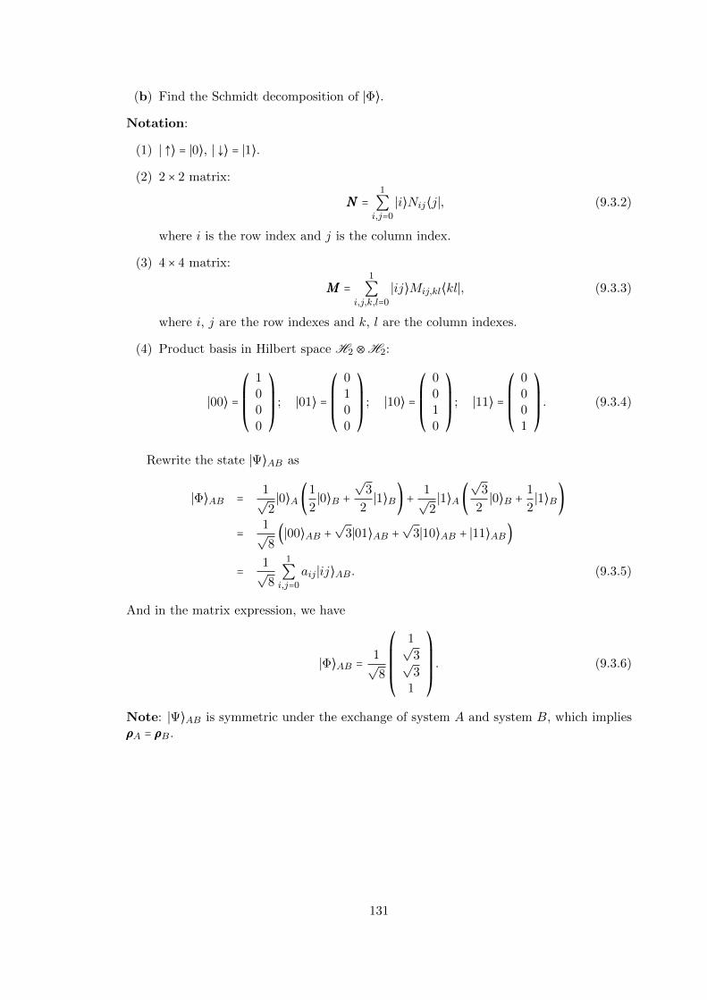
(b) Find the Schmidt decomposition of ∣Φ⟩.
Notation:
(1) ∣ ↑⟩ = ∣0⟩, ∣ ↓⟩ = ∣1⟩.
(2) 2 × 2 matrix:
NNN =1
∑i,j=0
∣i⟩Nij⟨j∣, (9.3.2)
where i is the row index and j is the column index.
(3) 4 × 4 matrix:
MMM =1
∑i,j,k,l=0
∣ij⟩Mij,kl⟨kl∣, (9.3.3)
where i, j are the row indexes and k, l are the column indexes.
(4) Product basis in Hilbert space H2 ⊗H2:
∣00⟩ =⎛⎜⎜⎜⎝
1000
⎞⎟⎟⎟⎠
; ∣01⟩ =⎛⎜⎜⎜⎝
0100
⎞⎟⎟⎟⎠
; ∣10⟩ =⎛⎜⎜⎜⎝
0010
⎞⎟⎟⎟⎠
; ∣11⟩ =⎛⎜⎜⎜⎝
0001
⎞⎟⎟⎟⎠. (9.3.4)
Rewrite the state ∣Ψ⟩AB as
∣Φ⟩AB = 1√2∣0⟩A (1
2∣0⟩B +
√3
2∣1⟩B) + 1√
2∣1⟩A (
√3
2∣0⟩B +
1
2∣1⟩B)
= 1√8(∣00⟩AB +
√3∣01⟩AB +
√3∣10⟩AB + ∣11⟩AB)
= 1√8
1
∑i,j=0
aij ∣ij⟩AB. (9.3.5)
And in the matrix expression, we have
∣Φ⟩AB = 1√8
⎛⎜⎜⎜⎜⎝
1√3√3
1
⎞⎟⎟⎟⎟⎠
. (9.3.6)
Note: ∣Ψ⟩AB is symmetric under the exchange of system A and system B, which impliesρρρA = ρρρB.
131

ρρρAB = ∣Ψ⟩AB⟨Ψ∣
=1
∑i,j,k,l=0
∣ij⟩AB⟨kl∣aija∗kl
=1
∑i,j,k,l=0
∣ij⟩AB⟨kl∣ρij,kl
= 1
8∣00⟩AB⟨00∣ +
√3
8∣00⟩AB⟨01∣ +
√3
8∣00⟩AB⟨10∣ + 1
8∣00⟩AB⟨11∣ (9.3.7)
+√
3
8∣01⟩AB⟨00∣ + 3
8∣01⟩AB⟨01∣ + 3
8∣01⟩AB⟨10∣ +
√3
8∣01⟩AB⟨11∣ (9.3.8)
+√
3
8∣10⟩AB⟨00∣ + 3
8∣10⟩AB⟨01∣ + 3
8∣10⟩AB⟨10∣ +
√3
8∣10⟩AB⟨11∣ (9.3.9)
+ 1
8∣11⟩AB⟨00∣ +
√3
8∣11⟩AB⟨01∣ +
√3
8∣11⟩AB⟨10∣ + 1
8∣11⟩AB⟨11∣. (9.3.10)
(9.3.11)
And in the matrix expression, we have
ρρρAB = 1
8
⎛⎜⎜⎜⎜⎝
1√3√3
1
⎞⎟⎟⎟⎟⎠
( 1√
3√
3 1 )
= 1
8
⎛⎜⎜⎜⎜⎝
1√
3√
3 1√3 3 3
√3√
3 3 3√
3
1√
3√
3 1
⎞⎟⎟⎟⎟⎠
. (9.3.12)
(a)
ρρρA = trBρρρAB
=1
∑m=0
B⟨m∣ρρρAB ∣m⟩B
=1
∑m=0
1
∑i,j,k,l=0
B⟨m∣ij⟩AB ρij,kl⟨kl∣m⟩B
=1
∑m=0
1
∑i,k=0
∣i⟩A⟨k∣ρim,km
= ( ρ00,00 + ρ01,01 ρ00,10 + ρ01,11
ρ10,00 + ρ11,01 ρ10,10 + ρ11,11)
= 1
8( 1 + 3
√3 +
√3√
3 +√
3 3 + 1)
= 1
2
⎛⎝
1√
32√
32 1
⎞⎠
= 1
2112 +
√3
4X, (9.3.13)
132

where X is the Pauli matrix,
X = σx = ( 0 11 0
) . (9.3.14)
ρρρB = trAρρρAB
=1
∑m=0
A⟨m∣ρρρAB ∣m⟩A
=1
∑m=0
1
∑i,j,k,l=0
A⟨m∣ij⟩AB ρij,kl⟨kl∣m⟩A
=1
∑m=0
1
∑i,k=0
∣j⟩B⟨l∣ρmj,ml
= ( ρ00,00 + ρ10,10 ρ00,01 + ρ10,11
ρ01,00 + ρ11,10 ρ01,01 + ρ11,11)
= 1
8( 1 + 3
√3 +
√3√
3 +√
3 3 + 1)
= 1
2
⎛⎝
1√
32√
32 1
⎞⎠
= 1
2112 +
√3
4X
= ρρρA. (9.3.15)
(b) Eigenstate of Pauli gate ZZZ.
ZZZ ∣0⟩ = ∣0⟩, ZZZ ∣1⟩ = −∣1⟩. (9.3.16)
Eigenstate of Pauli gate XXX.XXX ∣±⟩ = ±∣±⟩. (9.3.17)
⎧⎪⎪⎪⎪⎨⎪⎪⎪⎪⎩
∣±⟩ = 1√2(∣0⟩ ± ∣1⟩);
⟨+∣+⟩ = ⟨−∣−⟩ = 1, ⟨+∣−⟩ = ⟨−∣+⟩ = 0;III2 = ∣+⟩⟨+∣ + ∣−⟩⟨−∣.
(9.3.18)
Find the eigenstate of reduced density matrix ρρρA and ρρρB.
ρρρA,B ∣±⟩ = λ±∣±⟩, λ± =1
2±
√3
4, (9.3.19)
ρρρA,B = λ+∣+⟩A,B⟨+∣ + λ−∣−⟩A,B⟨−∣. (9.3.20)
Therefore
∣Ψ⟩AB = ∣+⟩A⟨+∣Ψ⟩AB + ∣−⟩A⟨−∣Ψ⟩AB= ∣+⟩A∣ϕ1⟩B + ∣−⟩A∣ϕ2⟩B, (9.3.21)
where
∣ϕ1⟩B =A ⟨+∣Ψ⟩AB =√
6 +√
2
4∣+⟩B =
√λ+∣+⟩B,
∣ϕ2⟩B =A ⟨−∣Ψ⟩AB = −√
6 −√
2
4∣−⟩B = −
√λ−∣−⟩B.
(9.3.22)
Thus, the Schmidt decomposition of state ∣Ψ⟩AB shows as
∣Ψ⟩AB =√λ+∣+⟩A∣+⟩B −
√λ−∣−⟩A∣−⟩B. (9.3.23)
133

9.4 The purification theorem and GHJW theorem
9.4.1 Purification
Thm 9.4.1.1 (Purification). For any given mixed state ρρρA for system A, there is a bipar-tite pure state ∣Φ⟩AB such that
ρρρA = trB( ∣Φ⟩AB ⟨Φ∣ ). (9.4.1)
Then ∣Φ⟩AB is called the purification of ρρρA.
For example, the density matrix
ρρρA = 1
2IIIA,
as we have shown in E.Q. (8.4.5), has the purification
∣ψ⟩AB = 1√2( ∣00⟩AB + ∣11⟩AB ).
Proof. The key point is the Schmidt decomposition. Suppose that
ρρρA ∶=∑i
pi ∣ϕi⟩A ⟨ϕi∣ , with ∑i
pi = 1,and pi > 0, (9.4.2)
where ∣ϕi⟩ is an orthonormal basis of HA.Now, we introduce another system B and construct the following state for the compositephysical system HA⊗HB,
∣Φ⟩AB =∑i
√pi ∣ϕi⟩A⊗ ∣αi⟩B , with ∑
i
pi = 1, (9.4.3)
amid, ∣αi⟩B is the orhonormal basis of HB. And we can show that ∣Φ⟩AB is a pure state,which is self-convincing, and it is also normalized since
AB ⟨Φ ∣Φ⟩AB = ∑i,j
√pjpi(A ⟨ϕj ∣⊗B ⟨αj ∣ )( ∣ϕi⟩A⊗ ∣αi⟩B )
= ∑i,j
√pipjA ⟨ϕj ∣ϕi⟩A B ⟨αj ∣αi⟩B
= ∑i,j
√pipjδijδij
= ∑i
pi
= 1.
We can also verify that ∣Φ⟩AB defined in E.Q. (9.4.3) is truly purification of the state ρρρA
as defined in E.Q. (9.4.2). As we can see that
trBρρρAB = ∑i
B ⟨αi∣ρρρAB ∣αi⟩B
= ∑i,j,k
√pjpkB ⟨αi∣ ( ∣ϕj⟩A⊗ ∣αj⟩B )(A ⟨ϕk∣⊗B ⟨αk∣ ) ∣αi⟩B
= ∑i,j,k
√pjpk( ∣ϕj⟩A ⟨ϕk∣ )⊗(B ⟨αi ∣αj⟩B ⟨αk ∣αi⟩B )
= ∑i,j,k
√pjpk( ∣ϕj⟩A ⟨ϕk∣ )δijδki
= ∑i
pi ∣ϕi⟩A ⟨ϕi∣
= ρρρA,
134
i.e.,ρρρA = trBρρρAB. (9.4.4)
Therefore, ∣Φ⟩AB is a purification of ρρρA.
There are some things that we should remark:
• ρρρA can be prepared as ensembles of pure states in many different ways. This can beinferred directly from the theorem of purification, since based on any state ensembleinterpretation of the ρρρA, we can always construct the corresponding purification,which can be different from each other.
• All these purification are experimentally indistinguishable, if one only observes thesystem A. Because for any measurement MMMA on the subsystem A, we have
⟨MMMA⟩ = trA(MMMAρρρA).
• Different purifications are associated with a local unitary transformation UUUB on thesubsystem B, which we will prove in the next subsection and introduce the GHJWtheorem.
9.4.2 The GHJW theorem
Thm 9.4.2.1 (GHJW). Consider many ensembles that realising ρρρA. There is a Hilbertspace HB and a bipartite pure state ∣Φ⟩AB, by which any one of these ensembles can berealized measuring a suitable observable of B.
Proof. Firstly, we would show that two arbitrary purification of ρρρA, e.g. ∣Φ⟩1 and ∣Φ⟩2,are connected with a local unitary transformation on the subsystem B. Let’s denote that
⎧⎪⎪⎨⎪⎪⎩
∣Φ1⟩A ∶= ∑i√pi ∣ϕi⟩A⊗ ∣αi⟩B ,
∣Φ2⟩A ∶= ∑i√qi ∣ψi⟩A⊗ ∣βi⟩B ,
(9.4.5)
where (pi, ∣ϕi⟩A) and (qi, ∣ψi⟩A) are two state ensemble interpretations of ρρρA and∣αi⟩B and ∣βi⟩B are two orthonormal basis for HB.Assume that ρρρA has the following eigenvectors and the associated eigenvalues
ρρρA ∣k⟩A = λk ∣k⟩A , with ∑k
λk = 1, and λk ≥ 0. (9.4.6)
Since ∣Φ1⟩AB and ∣Φ2⟩AB are two different purification of ρρρA, it’s apparent that
trA ∣Φ1⟩AB = trA ∣Φ2⟩AB = ρρρA. (9.4.7)
With E.Q. (9.4.7) in mind, we can see that the respective Schmidt decompositions for∣Φ1⟩AB and ∣Φ2⟩AB are
⎧⎪⎪⎨⎪⎪⎩
∣Φ1⟩AB = ∑k√λk ∣k⟩⊗ ∣k′1⟩B ,
∣Φ2⟩AB = ∑k√λk ∣k⟩⊗ ∣k′2⟩B .
(9.4.8)
Therefore, ∣Φ1⟩AB and ∣Φ2⟩AB are connected with the local unitary translation
∣Φ1⟩AB = (IIIA⊗UUUB) ∣Φ2⟩AB , (9.4.9)
135

withUUUB =∑
k
∣k′1⟩B⟨k′2∣ . (9.4.10)
Substitute E.Q. (9.4.5) into E.Q. (9.4.9), and we can get that
∣Φ1⟩AB =∑i
√qi ∣ψi⟩A⊗UUUB ∣βi⟩B ,
namely∣Φ1⟩AB =∑
i
√qi ∣ψi⟩A⊗ ∣γi⟩B , (9.4.11)
where∣γi⟩B ∶=UUUB ∣βi⟩B . (9.4.12)
Surely, ∣γi⟩B makes an orthonormal basis for HB, too.Secondly, let’s consider two observablesMMMB and NNNB defined in the subsystem B. And weconsider that case the two vector basis ∣αi⟩B and ∣γi⟩B respectively are eigenvectorsofMMMB and NNNB, namely
MMMB ∣αi⟩B = Mi ∣αi⟩B ,NNNB ∣γj⟩B = Nj ∣γj⟩B ,
with i, j = 1, . . .,dimHB.
Therefore, we can conclude that:
• After the measurement ofMMMB, there would be a probability of pi for the subsystemB in the state ∣αi⟩B, namely the subsystem A in the state ∣ϕi⟩A. Hence, measuringMMMB in the subsystem B would prepare the subsystem A in the mixed state ρρρA withthe state ensemble (pi, ∣ϕi⟩A).
• After the measurement of NNNB, there would be a probability of qj for the subsystemB in the state ∣γj⟩B, namely the subsystem A in the state of ∣ψi⟩A. Thus, themeasurement of NNNB in the subsystem B would prepare the subsystem A in themixed state ρρρA with the state ensemble (pi, ∣ψi⟩A).
Therefore, we get the GHJW theorem.
9.5 Information is physics
Ambiguities in the concept of density matrix
(a) A density matrix has many different interpretations of state ensemble.
(b) A density matrix can have many different interpretations of purification.
Here we discuss an example of bipartite system which is made up of two subsystemsAlice and Bob. Alice and Bob share a pure state of the form
∣ψ⟩AB = 1√2( ∣00⟩AB + ∣11⟩AB ). (9.5.1)
136

We can easily get the reduced density matrices for Alice and Bob respectively,
ρρρA = trBρρρAB
=1
∑i=0
B ⟨i∣ρρρAB ∣i⟩B
= 1
2
1
∑i,j,j′=0
B ⟨i∣ (∣j⟩A⊗ ∣j⟩B)(A ⟨j′∣⊗B ⟨j′∣) ∣i⟩B
= 1
2
1
∑i,j,j′=0
(∣j⟩A⊗B ⟨i ∣ j⟩B)(A ⟨j′∣⊗B ⟨j′ ∣ i⟩B)
= 1
2
1
∑i,j,j′=0
∣j⟩A ⟨j′∣ δijδj′i
= 1
2
1
∑i=0
∣i⟩A ⟨i∣ ,
i.e.,
ρρρA = 1
2III2. (9.5.2)
Reasoning in the same manner, we can get
ρρρB = 1
2III2. (9.5.3)
Now, let’s consider the following processes:
• The first process:
– Bob performs a measurement along the z-direction on his system but doesn’t tellAlice via classical communication (e.g. phone call). Therefore, no informationtransfer between Alice and Bob. In this case, we can get ρρρA = 1
2III2, which is amixed state.
– Bob performs a measurement along the z-direction on his system and phonecalls Alice about his measurement result (e.g. ∣0⟩B). There is informationtransferred between Alice and Bob. And, in this case ρρρA = ∣0⟩A ⟨0∣, which is apure state.
From this process, we can conclude that information (via classical communication)changes the physics of the system of Alice.
• The second process:
– Bob measures his qubit along the z-axis, and phone calls Alice but only tellsher that he has measured his qubit along the z-direction. Therefore, Alice’ssystem is prepared in state ensemble
(1
2, ∣0⟩) ,(1
2, ∣1⟩) . (9.5.4)
– Bob measures his qubit along the x-axis, and phone calls Alice but only tellsher that he has measured his qubit along the x-direction. Therefore, Alice’ssystem is prepared in state ensemble
(1
2, ∣+⟩) ,(1
2, ∣−⟩) . (9.5.5)
137

The two state ensembles described by (9.5.4) and (9.5.5) respectively, are not dis-tinguished by any conceivable measurement on the subsystem A only. The reason isthat both these two state ensemble are corresponding to the same density operatorρρρA = 1
2III2.
138

Chapter 10
Mixed State Entanglement andMulti-partite Entanglement
⋯ entanglement is a fundamentally new resource in the world that goes essen-tially beyond classical resources; iron to the classical world’s bronze age.
—Nielsen & Chuang
A major task of quantum computation and quantum information is to beexploit this new resource (quantum entanglement) to do information processingtasks impossibility or much more difficult with classical information.
—Nielsen & Chuang
A lot of mileage in quantum computation, and especially quantum information,has come from asking the simple question: “what would some entanglementbuy me in this problem?”.
—Nielsen & Chuang
References:
[Preskill] Chapter 4: Quantum entanglement;
[Nielsen & Chuang] Chapter 12: Quantum information theory.
10.1 Bipartite mixed state entanglement
10.1.1 Separability
10.1.1.1 Bipartite pure states
A bipartite pure state is separable if it is a tensor product of two pure states, i.e.,
∣ψ⟩AB = ∣α⟩A⊗ ∣β⟩B , (10.1.1)
which is equivalent to say that the bipartite pure state has the Schmidt number as 1 isseparable.
139

10.1.1.2 Bipartite mixed state
A bipartite mixed state ρρρAB is separable if it admits the ensemble description given by
ρρρAB =∑i,j
pijρρρA,i⊗ρρρB,j , (10.1.2)
where
∑i,j
pij = 1, pij ≥ 0
and ρρρA,i ∣ ∀ i are density operators for subsystem A, while ρρρB,j ∣ ∀ j for subsystem B.Example: This is a separable mixed state
ρρρAB =∑i
pi∣αi⟩ ⟨αi∣⊗∑j
qj ∣βj⟩ ⟨βj ∣ (10.1.3)
where pij = piqj∑i
pi = 1, with pi ≥ 0, ∀i,
and
∑i
qj = 1, with qj ≥ 0, ∀j.
10.1.2 Quantum bipartite entanglement
A bipartite state is entangled if it is not a separable state. Here is one separable state
ρρρ1 =1
4I2⊗I2. (10.1.4)
And another separable state shows as
ρρρ2 = 1
4
1
∑i=0
∣i⟩A ⟨i∣⊗1
∑j=0
∣j⟩B ⟨j∣
= 1
4
1
∑i,j=0
∣ij⟩AB ⟨ij∣
= 1
4(∣00⟩AB ⟨00∣ + ∣01⟩AB ⟨01∣ + ∣10⟩AB ⟨10∣ + ∣11⟩AB ⟨11∣). (10.1.5)
And for the state ρρρ3, is expressed as
ρρρ3 =1
4(∣φ+⟩ ⟨φ+∣ + ∣φ−⟩ ⟨φ−∣ + ∣ψ+⟩ ⟨ψ+∣ + ∣ψ−⟩ ⟨ψ−∣), (10.1.6)
which is hard to determine whether it is separable or entangled.However, as we shall see that ρρρ1, ρρρ2 and ρρρ3 are actually same, since both four product
states ∣ij⟩ ∣ i, j = 0,1 and four Bell states ∣ψ(ij)⟩ ∣ i, j = 0,1 can span the Hilbert spaceH2⊗H2, namely
ρρρ1 = ρρρ2 = ρρρ3. (10.1.7)
Remarks: Quantum entanglement is a very important but difficult issue in quantumphysics. How to quantify multi-particle entanglement is an open problem up to now.
140

10.1.3 Positive-partial transpose (PPT) criterion for quantum bipartiteseparability
Thm 10.1.3.1. If ρρρAB is separable, namely be of the form (10.1.2), then the partialtranspose of ρρρAB, defined as
(ρρρAB)PT
= (I2⊗T )ρρρAB
= ∑i,j
pijρρρA,i⊗(ρρρB,j)T, (10.1.8)
is still non-negative, where T denotes the transpose of matrix, namely
T ( ∣i⟩ ⟨j∣ ) = ∣j⟩ ⟨i∣ . (10.1.9)
Proof. As we shall know that ρρρB,j ∣ ∀ j are density operators of the subsystem B. There-fore, for an arbitrary ρρρB,j , the eigenvectors can span the local Hilbert space HB. If wecan diagonalize ρρρB,j with the basis being the complete set of independent orthonormaleigenvectors of ρρρB,j . After ρρρB,j being diagonalized, we can get that its transpose is diago-nalized, too. It would obvious that, that the transpose would preserve the eigenvalues ofρρρB,j . In another worlds, (ρρρB,j)T should also be nonnegative, namely
(ρρρB,j)T ≥ 0, ∀ j. (10.1.10)
On the other hand, the fact that ρρρA,i ∣ ∀ i being the density operators of the subsystem
A, ensures that they are all nonnegative. Therefore, (ρρρAB)PT
is nonnegative.
Corollary 10.1.3.1. If (ρρρAB)PT
is not positive, then ρρρAB is an entangled state.
This is a direct corollary of the theorem 10.1.3.1.
10.1.4 Example: the Werner state and the PPT criterion
Werner State, firstly presented in 1989 by Reinhard F. Werner, is defined as
ρρρ(λ) ∶= 1
4(1 − λ)I4 + λ∣φ+⟩ ⟨φ+∣ (10.1.11)
with λ being a real number. We can show that if ρρρ(λ) with definition (10.1.11) is a densitymatrix, iff
• Unit trace.
tr [ρρρ(λ)] = tr [1
4(1 − λ)I4 + λ∣φ+⟩ ⟨φ+∣]
= 1
4(1 − λ) tr (I4) + λtr (∣φ+⟩ ⟨φ+∣)
= (1 − λ) + λ= 1.
141
• Self-adjoint.
[ρρρ(λ)]† = [1
4(1 − λ)I4 + λ∣φ+⟩ ⟨φ+∣]
†
= [1
4(1 − λ)I4]
†+ (λ∣φ+⟩ ⟨φ+∣)†
= 1
4(1 − λ)∗I†
4 + λ∗ (∣φ+⟩ ⟨φ+∣)†
= 1
4(1 − λ)I4 + λ∣φ+⟩ ⟨φ+∣
= ρρρ(λ),
since λ ∈ R.
• Nonnegative.
ρρρ(λ) ≥ 0 ⇐⇒ the eigenvalues of ρρρ(λ) ≥ 0.
And it would be easy to verify that the Bell’s states ∣ψ(i, j)⟩ ∣ i, j = 1,2 are foureigenstates of ρρρ(λ).
ρρρ(λ) ∣ψ(0,0)⟩ = ρ(λ) ∣φ+⟩
= [1
4(1 − λ)I4 + λ∣ψ−⟩ ⟨ψ−∣] ∣φ+⟩
= 1
4(1 + 3λ) ∣φ+⟩ . (10.1.12)
and with i ≠ 0 and j ≠ 0, we can get
ρρρ(λ) ∣ψ(i, j)⟩ = ρρρ(λ) ∣ψ(i, j)⟩
= (1
4(1 − λ)I4 + λ∣ψ(0,0)⟩ ⟨ψ(0,0)∣) ∣ψ(i, j)⟩
= 1
4(1 − λ) ∣ψ(i, j)⟩ , (10.1.13)
as we know that ∣ψ(i, j)⟩, with (i, j = 0,1), are mutually independent. Therefore,we’ve gotten the complete set of mutually independent eigenvectors of ρρρ(λ).
Therefore, for the constrain of nonnegative:
ρρρ(λ) ≥ 0⇐⇒⎧⎪⎪⎪⎨⎪⎪⎪⎩
14(1 + 3λ) ≥ 0
14(1 − λ) ≥ 0
⇐⇒ −1
3≤ λ ≤ 1. (10.1.14)
When λ = −13
ρρρ(−1
3) = 1
3(I4 − ∣φ+⟩ ⟨φ+∣) = 1
3(∣φ−⟩⟨φ−∣ + ∣ψ+⟩⟨ψ+∣ + ∣ψ−⟩⟨ψ−∣),
therefore
ρρρ(−1
3) ∣φ+⟩ = 1
3(I4 − ∣φ+⟩ ⟨φ+∣)∣φ+⟩ = 0∣φ+⟩, (10.1.15)
142

and
ρρρ(−1
3) ∣ψ(i, j)⟩ = 1
3(I4 − ∣ψ(0,0)⟩ ⟨ψ(0,0)∣) ∣ψ(i, j)⟩ = 1
3∣ψ(i, j)⟩ (10.1.16)
with i ≠ 0 and j ≠ 0.When λ = 1
ρρρ(1) = ∣φ+⟩ ⟨φ+∣ ,which is a pure state with the relations
ρρρ (1) ∣φ+⟩ = (∣φ+⟩ ⟨φ+∣)∣φ+⟩ = ∣φ+⟩. (10.1.17)
andρρρ (1) ∣ψ(i, j)⟩ = (∣φ+⟩ ⟨φ+∣)∣ψ(i, j)⟩ = 0∣ψ(i, j)⟩ (10.1.18)
with i ≠ 0 and j ≠ 0.
Calculate the partial transpose of Werner state ρρρ(λ).
[ρρρ(λ)]PT = (I2⊗T )ρρρ(λ)
= (I2⊗T ) [1
4(1 − λ)I4 + λ∣φ+⟩ ⟨φ+∣]
= 1
4(1 − λ) (I2⊗T )I4 + λ(I2⊗T )∣φ+⟩ ⟨φ+∣
= 1
4(1 − λ)I4 +
1
2λ(I2⊗T ) (∣00⟩ ⟨00∣ + ∣00⟩ ⟨11∣ + ∣11⟩ ⟨00∣ + ∣11⟩ ⟨11∣)
= 1
4(1 − λ)I4 +
1
2λ (∣00⟩ ⟨00∣ + ∣01⟩ ⟨10∣ + ∣10⟩ ⟨01∣ + ∣11⟩ ⟨11∣) , (10.1.19)
from which we can see that
[ρρρ(λ)]PT ∣φ+⟩ = [ρρρ(λ)]PT ∣00⟩ + ∣11⟩√2
= [1
4(1 − λ) + 1
2λ] ∣φ+⟩
= 1
4(1 + λ) ∣φ+⟩ , (10.1.20)
[ρρρ(λ)]PT ∣φ−⟩ = [ρρρ(λ)]PT ∣00⟩ − ∣11⟩√2
= [1
4(1 − λ) + 1
2λ] ∣φ−⟩
= 1
4(1 + λ) ∣φ−⟩ , (10.1.21)
[ρρρ(λ)]PT ∣ψ+⟩ = [ρρρ(λ)]PT ∣01⟩ + ∣10⟩√2
= [1
4(1 − λ) + 1
2λ] ∣ψ+⟩
= 1
4(1 + λ) ∣ψ+⟩ , (10.1.22)
[ρρρ(λ)]PT ∣ψ−⟩ = [ρρρ(λ)]PT ∣01⟩ − ∣10⟩√2
= [1
4(1 − λ) − 1
2λ] ∣ψ−⟩
= 1
4(1 − 3λ) ∣ψ−⟩ . (10.1.23)
143

In another viewpoint, we can see
(112 ⊗TTT )∣φ+⟩⟨φ+∣ = (112 ⊗TTT )1
2
1
∑i,j=0
∣ii⟩⟨jj∣
= 1
2
1
∑i,j=0
(112 ⊗TTT )(∣i⟩⟨j∣⊗ ∣i⟩⟨j∣)
= 1
2
1
∑i,j=0
∣i⟩⟨j∣⊗TTT (∣i⟩⟨j∣)
= 1
2
1
∑i,j=0
∣i⟩⟨j∣⊗ ∣j⟩⟨i∣
= 1
2
1
∑i,j=0
∣ij⟩⟨ji∣
= 1
2SWAP (10.1.24)
where the Swap gate is defined in (6.2.4) and has the matrix expression
SWAP ≡1
∑i,j=0
∣ij⟩⟨ji∣ =⎛⎜⎜⎜⎝
1 0 0 00 0 1 00 1 0 00 0 0 1
⎞⎟⎟⎟⎠. (10.1.25)
Note that the SWAP gate is identical with its inverse, namely
SWAP SWAP = III4, (10.1.26)
which implies the characteristic equation
SWAP2 − III4 = 0. (10.1.27)
Thus, we can see the eigenvalue of the SWAP gate is ±1. In two electrons system, i.e., twospin-1
2 system, triplet states are eigenstate of SWAP gate with eigenvalue 1, expressed as
SWAP∣φ+⟩∣φ−⟩∣ψ+⟩
⎫⎪⎪⎪⎬⎪⎪⎪⎭=
∣φ+⟩∣φ−⟩∣ψ+⟩
⎫⎪⎪⎪⎬⎪⎪⎪⎭. (10.1.28)
For singlet state, it is the eigenstate of SWAP gate with eigenvalue −1,
SWAP∣ψ−⟩ = −∣ψ−⟩. (10.1.29)
Therefore, rewrite the SWAP gate as
SWAP = ∣φ+⟩⟨φ+∣ + ∣φ−⟩⟨φ−∣ + ∣ψ+⟩⟨ψ+∣ − ∣ψ−⟩⟨ψ−∣ = III4 − 2∣ψ−⟩⟨ψ−∣. (10.1.30)
And the partial transpose of Werner state ρρρ(λ) can be calculated as
[ρρρ(λ)]PT = (I2⊗T )ρρρ(λ)
= (I2⊗T ) [1
4(1 − λ)I4 + λ∣φ+⟩ ⟨φ+∣]
= 1
4(1 − λ)III4 +
λ
2SWAP
= 1
4(1 − λ)III4 +
1
2λIII4 − λ∣ψ−⟩⟨ψ−∣
= 1
4(1 + λ)III4 − λ∣ψ−⟩⟨ψ−∣. (10.1.31)
144

And the eigenvalues can be obtained by the way
[ρρρ(λ)]PT∣ψ−⟩ = (1
4(1 + λ) − λ)∣ψ−⟩ = 1 − 3λ
4∣ψ−⟩, (10.1.32)
[ρρρ(λ)]PT∣φ+⟩∣φ−⟩∣ψ+⟩
⎫⎪⎪⎪⎬⎪⎪⎪⎭= 1
4(1 + λ)
∣φ+⟩∣φ−⟩∣ψ+⟩
⎫⎪⎪⎪⎬⎪⎪⎪⎭. (10.1.33)
Therefore, ρρρ(λ) has the eigenvalues 14(1 + λ),
14(1 − 3λ), and the eigenstates
∣φ+⟩ , ∣φ−⟩ , ∣ψ+⟩´¹¹¹¹¹¹¹¹¹¹¹¹¹¹¹¹¹¹¹¹¹¹¹¹¹¹¹¹¹¹¹¹¹¹¹¹¹¹¸¹¹¹¹¹¹¹¹¹¹¹¹¹¹¹¹¹¹¹¹¹¹¹¹¹¹¹¹¹¹¹¹¹¹¹¹¹¹¶14(1+λ), triplet state
, ∣ψ−⟩±
14(1−3λ), singlet state
. (10.1.34)
For the partial transpose criterion, we have the constrain for the parameter λ
[ρρρ(λ)]PT ≥ 0⇐⇒⎧⎪⎪⎪⎨⎪⎪⎪⎩
14(1 + λ) ≥ 0
14(1 − 3λ) ≥ 0
⇐⇒ −1 ≤ λ ≤ 1
3. (10.1.35)
From inequality (10.1.14) and inequality (10.1.35), we can infer that
ρρρ(λ) ≥ 0 ⇐⇒ −1
3≤ λ ≤ 1,
[ρρρ(λ)]PT ≥ 0 ⇐⇒ −1 ≤ λ ≤ 1
3.
That means
ρρρ(λ) is separable ⇐⇒ −1
3≤ λ≤ 1
3,
ρρρ(λ) is entangled ⇐⇒ 1
3< λ≤1.
10.1.5 Example: the Werner state and the CHSH inequality
Now let’s consider the CHSH inequality for the bipartite Werner states. We may set thefour observables to be A = σσσA⋅a1 and B = σσσA⋅a2 in subsystem Alice, and C = σσσB ⋅b1 andD = σσσB ⋅b2 in subsystem Bob.Firstly, we can calculate
⟨(σσσA⋅a) (σσσB ⋅b)⟩ = trAB [(σσσA⋅a) (σσσB ⋅b)ρρρ(λ)]
= trAB [(σσσA⋅a) (σσσB ⋅b)(1
4(1 − λ)III4 + λ ∣φ+⟩ ⟨φ+∣)]
= 1 − λ4
trA (σσσA⋅a) trB (σσσB ⋅b) + λ ⟨φ+∣ (σσσA⋅a) (σσσB ⋅b) ∣φ+⟩
= λ ⟨φ+∣ (σσσA⋅a) (σσσB ⋅b) ∣φ+⟩= λa⋅b. (10.1.36)
Therefore, we can get
∣ ⟨ACACAC⟩ + ⟨BCBCBC⟩ + ⟨ADADAD⟩ − ⟨BDBDBD⟩ ∣ = ∣λ∣ ∣a1 ⋅b1 + a2 ⋅b1 + a1 ⋅b2 − a2 ⋅b2∣= ∣λ∣ ∣(a1 + a2)⋅b1 + (a1 − a2)⋅b2∣ . (10.1.37)
145

Since (a′1 + a′2) and (a′1 − a′2) are mutually orthogonal,therefore
0 ≤ ∣(a1 + a2)⋅b1 + (a1 − a2)⋅b2∣ ≤ 2√
2. (10.1.38)
To ensure the CHSH inequality
∣ ⟨ACACAC⟩ + ⟨BCBCBC⟩ + ⟨ADADAD⟩ − ⟨BDBDBD⟩ ∣ ≤ 2 (10.1.39)
being correct, we only need
∣ ⟨ACACAC⟩ + ⟨BCBCBC⟩ + ⟨ADADAD⟩ − ⟨BDBDBD⟩ ∣max ≤ 2, (10.1.40)
i.e.,
2√
2∣λ∣ ≤ 2, ⇐⇒ − 1√2≤ λ ≤ 1√
2. (10.1.41)
Combine above constrain of parameter λ with the inequality (10.1.14) which ensures ρρρ(λ)nonnegative namely a density operator, and we can get
−1
3≤ λ ≤ 1√
2. (10.1.42)
As we shall see that with λ ∈ [−1/3,1], the operator ρρρ(λ) is ensured to be a possible densityoperator, and
• if λ ∈ (1/3,1], the Werner state ρρρ(λ) is entangled;
• if λ ∈ [−1/3,1/√
2],the Werner state ρρρ(λ) obeys the CHSH inequality;
• if λ ∈ [1/3,1/√
2], the Werner state ρρρ(λ) is entangled but compatible with the CHSHinequality.
Since the CHSH inequality is actually a kind of Bell’s inequality, which is the criterion oflocal hidden variable theorem, we can conclude that entanglement is not always contra-dicted with the local hidden variable theorem, namely the entanglement can exist in thelocal hidden variable theory in some case.
10.2 Multi-partite entanglement
10.2.1 Definition
Def 10.2.1. We define the multi-partite separability and entanglement in the following.
1 The N -partite state is fully separable iff
• Pure state:∣ψ⟩A1A2⋯An
= ∣ψ⟩A1⊗ ∣ψ⟩A2
⊗⋯⊗ ∣ψ⟩An; (10.2.1)
• Mixed state:ρρρA1A2⋯An =∑
i=1
piρρρiA1⊗ρρρiA2
⊗⋯⊗ρρρiAn . (10.2.2)
• A fully separable tripartite is shown in a diagram form in Figure 10.1, wherethe dashed lines represent separable states and Ai denote the i-th particle, withi = 1,2,3.
146

A1
A2 A3
Figure 10.1: Fully separable tripartite
A2
A1
A3
(a)
A2
A1
A3
(b)
A1
A2 A3
(c)
Figure 10.2: Full entangled tripartite
2 N -partite fully entangled iff it’s not fully separable. We can also represent this ina diagram. We still take the tripartite system as an example, as shown in Figure10.2 are the three cases of the fully entangled tripartite state, where the solid linesrepresents the entangled states.
3 N -partite genuinely entangled iff all bipartite partitions are entangled. We can takethe tripartite for an example, as shown in Figure 10.3.
A1
A2 A3
Figure 10.3: Genuinely entangled tripartite
10.2.2 The GHZ state
Def 10.2.2 (N -qubit GHZ states). The state defined as
∣GHZ±⟩N = 1√2( ∣x⟩± ∣x⟩ ), (10.2.3)
is the so called N -qubit GHZ state, where x is an N -bit string of 0 and 1 and x + x =(1 0⋯0
±N
)binary
.
From this definition we can see that
1 n = 1:
∣±⟩ = 1√2(∣0⟩± ∣1⟩) ,
which are eigenstates of XXX with eigenvalues of ±1;
147

2 n = 2:
∣ψ(0,0)⟩= 1√2(∣00⟩ + ∣11⟩)
∣ψ(0,1)⟩= 1√2(∣00⟩ − ∣11⟩)
∣ψ(1,0)⟩= 1√2(∣01⟩ + ∣10⟩)
∣ψ(1,1)⟩= 1√2(∣01⟩ − ∣10⟩)
⎫⎪⎪⎪⎪⎪⎪⎪⎪⎪⎪⎪⎪⎪⎪⎪⎪⎬⎪⎪⎪⎪⎪⎪⎪⎪⎪⎪⎪⎪⎪⎪⎪⎪⎭
⇐⇒ Bell states ∣φ±⟩ , ∣ψ±⟩ ,
all of which are eigenvectors of the parity-bit operator ZZZ⊗ZZZ and that of the phase-bitoperator XXX⊗XXX.
3 n = 3:⎧⎪⎪⎪⎪⎪⎪⎪⎪⎪⎪⎪⎪⎪⎪⎪⎪⎨⎪⎪⎪⎪⎪⎪⎪⎪⎪⎪⎪⎪⎪⎪⎪⎪⎩
∣Φ1⟩=1√2( ∣000⟩ + ∣111⟩ ), ∣Φ8⟩=
1√2( ∣000⟩ − ∣111⟩ ),
∣Φ2⟩=1√2( ∣001⟩ + ∣110⟩ ), ∣Φ7⟩=
1√2( ∣001⟩ − ∣110⟩ ),
∣Φ3⟩=1√2( ∣010⟩ + ∣101⟩ ), ∣Φ6⟩=
1√2( ∣010⟩ − ∣101⟩ ),
∣Φ4⟩=1√2( ∣011⟩ + ∣100⟩ ), ∣Φ5⟩=
1√2( ∣011⟩ − ∣100⟩ ),
with the phase-bit operator XXX⊗XXX⊗XXX and
• 1st parity-bit operator: ZZZ⊗ZZZ⊗III2,
• 2nd parity-bit operator: III2⊗ZZZ⊗ZZZ.
4 n-qubit: ∣GHZ⟩n =1√2( ∣00⋯0²
n
⟩ + ∣11⋯1²
n
⟩ ), with n observables
nobservables
⎧⎪⎪⎪⎪⎪⎪⎪⎪⎪⎪⎪⎪⎪⎪⎪⎪⎪⎪⎪⎪⎨⎪⎪⎪⎪⎪⎪⎪⎪⎪⎪⎪⎪⎪⎪⎪⎪⎪⎪⎪⎪⎩
phase-bit ∶ XXX⊗XXX⊗⋯⊗XXX´¹¹¹¹¹¹¹¹¹¹¹¹¹¹¹¹¹¹¹¹¹¹¹¹¹¹¹¹¹¹¹¸¹¹¹¹¹¹¹¹¹¹¹¹¹¹¹¹¹¹¹¹¹¹¹¹¹¹¹¹¹¹¹¹¶
n
,
1st parity-bit ∶ ZZZ⊗ZZZ⊗III2⊗⋯⊗III2´¹¹¹¹¹¹¹¹¹¹¹¹¹¹¹¹¹¸¹¹¹¹¹¹¹¹¹¹¹¹¹¹¹¹¹¹¶
n−2
,
2nd parity-bit ∶ III2⊗ZZZ⊗ZZZ⊗III2⊗⋯⊗III2´¹¹¹¹¹¹¹¹¹¹¹¹¹¹¹¹¹¸¹¹¹¹¹¹¹¹¹¹¹¹¹¹¹¹¹¹¶
n−3
,
⋮(n − 1)-th parity-bit ∶ III2⊗III2⊗⋯⊗III2
´¹¹¹¹¹¹¹¹¹¹¹¹¹¹¹¹¹¹¹¹¹¹¹¹¹¹¹¹¹¹¹¹¸¹¹¹¹¹¹¹¹¹¹¹¹¹¹¹¹¹¹¹¹¹¹¹¹¹¹¹¹¹¹¹¹¹¶n−2
⊗ZZZ⊗ZZZ;
(XXX1⊗XXX2⊗⋯⊗XXXn) ∣GHZ⟩n= (XXX1⊗XXX2⊗⋯⊗XXXn)
1√2[∣0x2x3⋯xn⟩ + (−1)x1 ∣1x2x3⋯xn⟩]
= 1√2[ ∣1x2x3⋯xn⟩ + (−1)x1 ∣0x2x3⋯xn⟩ ]
= (−1)x1 1√2[ ∣0x2x3⋯xn⟩ + (−1)x1 ∣1x2x3⋯xn⟩ ]
= (−1)x1 ∣GHZ⟩n .
148

[ZZZ1⊗ZZZ2⊗III2⊗⋯⊗III2´¹¹¹¹¹¹¹¹¹¹¹¹¹¹¹¹¹¸¹¹¹¹¹¹¹¹¹¹¹¹¹¹¹¹¹¹¶
n−2
] ∣GHZ⟩n
= [ZZZ1⊗ZZZ2⊗III2⊗⋯⊗III2´¹¹¹¹¹¹¹¹¹¹¹¹¹¹¹¹¹¸¹¹¹¹¹¹¹¹¹¹¹¹¹¹¹¹¹¹¶
n−2
] 1√2( ∣0x2x3⋯xn⟩ + (−1)x1 ∣1x2x3⋯xn⟩ )
= 1√2[(−1)x2 ∣0x2x3⋯xn⟩ + (−1)x1(−1)(−1)x2+1 ∣1x2x3⋯xn⟩ ]
= (−1)x2 1√2[ ∣0x2x3⋯xn⟩ + (−1)x1 ∣1x2x3⋯xn⟩ ]
= (−1)x2 ∣GHZ⟩n .
(III2⊗ZZZ2⊗ZZZ3⊗III2⊗III2´¹¹¹¹¸¹¹¹¹¶n−3
) ∣GHZ⟩n
= (III2⊗ZZZ2⊗ZZZ3⊗III2⊗III2´¹¹¹¹¸¹¹¹¹¶n−3
) 1√2[ ∣0x2x3⋯xn⟩ + (−1)x1 ∣1x2x3⋯xn⟩ ]
= 1√2[(−1)x2+x3 ∣0x2x3⋯xn⟩ + (−1)x1(−1)x2+1(−1)x3+1 ∣1x2x3⋯xn⟩ ]
= (−1)x2+x3 1√2[ ∣0x2x3⋯xn⟩ + (−1)x1 ∣1x2x3⋯xn⟩ ]
= (−1)x2+x3 ∣GHZ⟩n .
(III2⊗III2⊗ZZZ3⊗ZZZ4⊗III2⊗⋯⊗III2´¹¹¹¹¹¹¹¹¹¹¹¹¹¹¹¹¹¸¹¹¹¹¹¹¹¹¹¹¹¹¹¹¹¹¹¹¶
n−4
) ∣GHZ⟩n
= (III2⊗III2⊗ZZZ3⊗ZZZ4⊗III2⊗⋯⊗III2´¹¹¹¹¹¹¹¹¹¹¹¹¹¹¹¹¹¸¹¹¹¹¹¹¹¹¹¹¹¹¹¹¹¹¹¹¶
n−4
) 1√2[ ∣0x2x3⋯xn⟩ + (−1)x1 ∣1x2x3⋯xn⟩ ]
= 1√2[(−1)x3+x4 ∣0x2x3⋯xn⟩ + (−1)x1(−1)x3+1(−1)x4+1 ∣1x2x3⋯xn⟩ ]
= (−1)x3+x4 1√2[ ∣0x2x3⋯xn⟩ + (−1)x1 ∣1x2x3⋯xn⟩ ]
= (−1)x3+x4 ∣GHZ⟩n .
(III2⊗⋯⊗III2´¹¹¹¹¹¹¹¹¹¹¹¹¹¹¹¹¹¸¹¹¹¹¹¹¹¹¹¹¹¹¹¹¹¹¹¹¶
n−2
⊗ZZZn−1⊗ZZZn) ∣GHZ⟩n
= (III2⊗⋯⊗III2´¹¹¹¹¹¹¹¹¹¹¹¹¹¹¹¹¹¸¹¹¹¹¹¹¹¹¹¹¹¹¹¹¹¹¹¹¶
n−2
⊗ZZZn−1⊗ZZZn)1√2[ ∣0x2x3⋯xn⟩ + (−1)x1 ∣1x2x3⋯xn⟩ ]
= 1√2[(−1)xn−1+xn ∣0x2x3⋯xn⟩ + (−1)x1(−1)xn−1+1(−1)xn+1 ∣1x2x3⋯xn⟩ ]
= (−1)xn−1+xn 1√2[ ∣0x2x3⋯xn⟩ + (−1)x1 ∣1x2x3⋯xn⟩ ]
= (−1)xn−1+xn ∣GHZ⟩n .
149

We can then conclude that with the input qubit ∣x1x2⋯xn⟩, we can get the outputqubit ∣GHZ⟩n which is the common eigenvector of the phase-bit operator, the 1stparity-bit operator, the 2nd parity-bit operator, ⋯ and the (n − 1)-th parity bitoperator, with the corresponding eigenvalues (x1, x2, x2 + x3,⋯, xn−1 + xn).
5 n → large number,
∣GHZ⟩n =1√2(∣live⟩ + ∣dead⟩) (cat state),
which means the macroscopically distinguished states used in Schrodinger’s cat ex-periment.
10.2.3 Properties of GHZ states
1 For the GHZ states ∣GHZ±⟩, each qubit is maximally entangled with the other n− 1qubit, e.g.
ρρρA1∶= trA2A3⋯An ∣GHZ±⟩n ⟨GHZ±∣
= 1
2trA2A3⋯An( ∣0y⟩n ± ∣1y⟩n )(n ⟨0y∣±n ⟨1y∣ ),
with y being a (n − 1)-bit string of 0 and 1, thus
ρρρA1 = 1
2∑y′
A2A3⋯An ⟨y′∣ ( ∣0y⟩n ± ∣1y⟩n )(n ⟨0y∣±n ⟨1y∣ ) ∣y′⟩A2A3⋯An
= 1
2∑y′
( ∣0⟩ δy′y± ∣1⟩ δy′y)( ⟨0∣ δyy′± ⟨1∣ δyy′)
= 1
2( ∣0⟩ ⟨0∣ + ∣1⟩ ⟨1∣ ),
i.e.
ρρρA1 =1
2III2. (10.2.4)
2 Cutting one-qubit gives rise to separable (n − 1)-qubit mixed state with rank 2.
ρρρA2⋯An = trA1 ∣GHZ±⟩n ⟨GHZ±∣
= 1
2
1
∑i=0
A1 ⟨i∣ ( ∣0y⟩n + ∣1y⟩n )(n ⟨0y∣ + n ⟨1 ⟨y∣∣ ) ∣i⟩A1
namely
ρρρA2⋯An =1
2( ∣y⟩n−1 ⟨y∣ + ∣y⟩n−1 ⟨y∣), (10.2.5)
from which it would be obvious that ρρρA2⋯An can be rewritten in the form as illus-trated in E.Q. (10.2.2), namely ρρρA2⋯An is separable. Note that we can apply thePPT criterion in this case since
ρρρPTA2⋯An = (Id⊗ T )ρρρA2⋯An = ρρρA2⋯An ≥ 0 (10.2.6)
which is the necessary condition for quantum separability.
3 n-qubit GHZ states ∣GHZ±⟩n =12 form an orthonormal basis of n-qubit Hilber space,
i.e.
4 Given a n-qubit ∣GHZ⟩n, other (2n−1) ∣GHZ±⟩n states can be generated via LOCC,e.g. for the case of n = 2, the other Bell states can be get from ∣φ+⟩, as shown inFigure 10.4
150

Table 10.1: ∣GHZ±⟩n makes an orthonormal basis for n-qubit Hilbert space.
n GHZ states (orthnormal basis) n-qubit Hilbert space
n = 1 ∣±⟩ H2
n = 2 ∣ψ(i, j)⟩ , i, j = 0,1 H2⊗H2
n = 3 ∣Φi⟩ , i = 1,2,⋯,8 H2⊗H2⊗H2
⋮
n ∣GHZ±⟩n H2⊗H2⊗⋯⊗H2´¹¹¹¹¹¹¹¹¹¹¹¹¹¹¹¹¹¹¹¹¹¹¹¹¹¹¹¹¹¹¹¹¹¹¹¹¹¹¹¹¹¹¹¹¸¹¹¹¹¹¹¹¹¹¹¹¹¹¹¹¹¹¹¹¹¹¹¹¹¹¹¹¹¹¹¹¹¹¹¹¹¹¹¹¹¹¹¹¹¹¶
n
∣φ+⟩III 4
∣φ+⟩III 2⊗ZZZ
∣φ−⟩
III2⊗XXX
∣ψ+⟩
III2⊗XZXZXZ
∣ψ−⟩
Figure 10.4: Bell states generated from ∣φ+⟩
151
Part IV
Quantum Open System andQuantum Error Correction Codes
152

Chapter 11
Quantum Mechanics (III):Quantum Open System
Real systems suffer from unwanted interactions with the outside world. Theseunwanted interactions show up as noise in quantum information processingsystems. We need to understand and control such noise processes in order tobuild useful quantum information processing systems.
—Nielsen & Chuang
No quantum systems are ever perfectly closed, and especially not quantumcomputers, which must be delicately programmed by an external system toperform some desired set of operations.
—Nielsen & Chuang
An open system is nothing more than one which has interactions with someother environment system, whose dynamics we wish to neglect or average over.
—Nielsen & Chuang
The mathematical formalism of quantum operations is the key tool for ourdescription of the dynamics of open quantum systems.
—Nielsen & Chuang
Another advantage of quantum operations in applications to quantum com-putation and quantum information is that they are especially well adaptedto describe discrete state changes, that is, transformations between an initialstate ρ and ρ′, without explicit reference to the passage of time.
—Nielsen & Chuang
We will construct an artificial example of a system whose evolution is notdescribed by a quantum operation, ⋯. It is an interesting problem for furtherstudy to study quantum information processing beyond the quantum operationformalism.
—Nielsen & Chuang
References:
[Preskill] Chapter 2: Foundations II: measurement and evolution;
[Nielsen & Chuang] Chapter 8: Quantum noise and quantum operation.
153
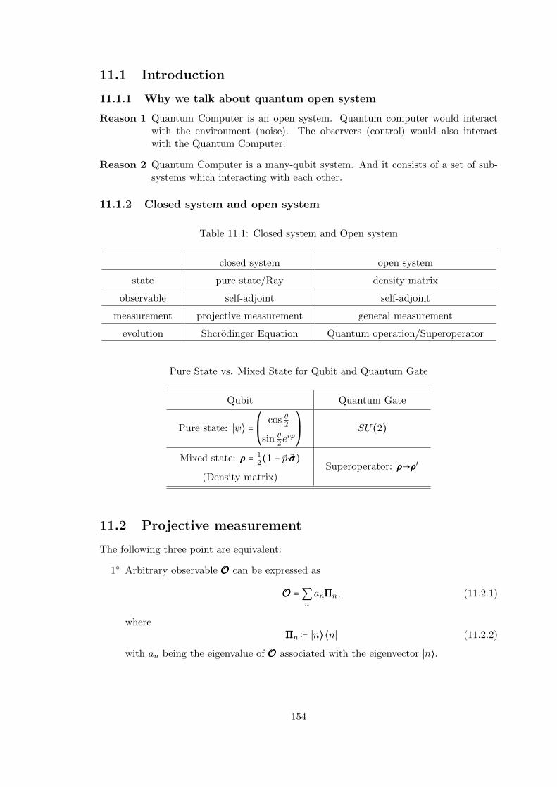
11.1 Introduction
11.1.1 Why we talk about quantum open system
Reason 1 Quantum Computer is an open system. Quantum computer would interactwith the environment (noise). The observers (control) would also interactwith the Quantum Computer.
Reason 2 Quantum Computer is a many-qubit system. And it consists of a set of sub-systems which interacting with each other.
11.1.2 Closed system and open system
Table 11.1: Closed system and Open system
closed system open system
state pure state/Ray density matrix
observable self-adjoint self-adjoint
measurement projective measurement general measurement
evolution Shcrodinger Equation Quantum operation/Superoperator
Pure State vs. Mixed State for Qubit and Quantum Gate
Qubit Quantum Gate
Pure state: ∣ψ⟩ =⎛⎜⎝
cos θ2
sin θ2eiϕ
⎞⎟⎠
SU(2)
Mixed state: ρρρ = 12(1 + p⋅σσσ) Superoperator: ρρρ→ρρρ′
(Density matrix)
11.2 Projective measurement
The following three point are equivalent:
1 Arbitrary observable OOO can be expressed as
OOO =∑n
anΠΠΠn, (11.2.1)
whereΠΠΠn ∶= ∣n⟩ ⟨n∣ (11.2.2)
with an being the eigenvalue of OOO associated with the eigenvector ∣n⟩.
154

The mean value of the observable should be
⟨OOO⟩ = ⟨ψ ∣OOO ∣ψ⟩= ⟨ψ∣∑
n
anΠΠΠn∣ψ⟩
= ∑n
an ⟨ψ ∣n⟩ ⟨n ∣ψ⟩
= ∑n
anPn, (11.2.3)
withPn ∶= ∣ ⟨ψ ∣n⟩ ∣2 (11.2.4)
2 In the orthonormal basis ∣n⟩, observables can be determined by the basis.
The probability, that the post-measurement is ∣n⟩, should be
Prob(n) = ∣⟨n ∣ψ⟩∣2
= ⟨ψ ∣n⟩ ⟨n ∣ψ⟩= ⟨ψ ∣ΠΠΠn ∣ψ⟩= tr(ρρρΠΠΠn). (11.2.5)
The post-measurement state should be
∣ψ⟩ → ∣n⟩ ⟨n∣ψ⟩√Prob(n)
, (11.2.6)
or
ρρρ ∶= ∣ψ⟩ ⟨ψ∣ → ΠΠΠn ∣ψ⟩ ⟨ψ∣ΠΠΠ†n
Prob(n)= ΠΠΠnρρρΠΠΠn
Prob(n). (11.2.7)
That is for the pure state.
3 Complete set of orthogonal projection ΠΠΠn.
And we know that ΠΠΠn should satisfy
⎧⎪⎪⎪⎪⎪⎪⎪⎪⎨⎪⎪⎪⎪⎪⎪⎪⎪⎩
ΠΠΠnΠΠΠm = δmn,orthonormal;
ΠΠΠ†n = ΠΠΠn, Hermition;
∑n
ΠΠΠn = Id, completeness.
(11.2.8)
Now, if we consider a mixed state described by the density matrix, then
ρρρ → ρρρ′ =∑n
Prob(n) ΠΠΠnρρρΠΠΠn
Prob(n)=∑
n
ΠΠΠnρρρΠΠΠn (11.2.9)
which defines the ensemble
ρρρ′ = Prob(n), ΠΠΠnρρρΠΠΠn
Prob(n)
.Example: A single-qubit density matrix is defined as
ρρρ(p) ∶= 1
2(1 + p⋅σσσ) , with p ∈ R3, and 0 ≤ ∥p∥ ≤ 1. (11.2.10)
155

The projectors are defined as,
⎧⎪⎪⎪⎪⎨⎪⎪⎪⎪⎩
ΠΠΠ1 ∶=1
2(1 + n⋅σσσ) = ∣n⟩ ⟨n∣ , (11.2.11a)
ΠΠΠ2 ∶=1
2(1 − n⋅σσσ) = ∣−n⟩ ⟨−n∣ . (11.2.11b)
It would be obvious that⎧⎪⎪⎪⎨⎪⎪⎪⎩
ΠΠΠ1 +ΠΠΠ2 = Id,ΠΠΠiΠΠΠj = δijId,
ΠΠΠ†i = ΠΠΠi.
(11.2.12)
The probabilities that the post-measurement state should be ∣n⟩, and that for ∣−n⟩, are
⎧⎪⎪⎪⎪⎨⎪⎪⎪⎪⎩
P1 = tr(ρρρΠΠΠ1) =1
2(1 + p⋅n) , (11.2.13a)
P2 = tr(ρρρΠΠΠ2) =1
2(1 − p⋅n) (11.2.13b)
11.3 General measurement theory
1 Measurement operators
• measurement operators MMMm;
• the measurements can be represented by measurement operators;
• measurement operator MMMm is labeled by m;
• completeness relation ∑mMMM†mMMMm = Id.
The projectors is defined asΠΠΠn ∶= ∣n⟩ ⟨n∣ . (11.3.1)
The measurement operatorsMMMn ∶=ΠΠΠn. (11.3.2)
Therefore,MMM †
nMMMn = ΠΠΠn (11.3.3)
namely
∑n
MMM †nMMMn = ∑
n
ΠΠΠn
= ∑n
∣n⟩ ⟨n∣
= Id. (11.3.4)
2 State
• pure state ∣ψ⟩;• mixed state ρρρ.
3 Measurement statistics
• pure state: Prob(m) = ⟨ψ∣MMM †mMMMm ∣ψ⟩;
• mixed state: Prob(m) = tr (MMM †mMMMmρρρ);
156
4 total probability:
• pure state:
∑m
Prob(m) = ∑m
⟨ψ∣MMM †mMMMm ∣ψ⟩
= ⟨ψ∣∑m
MMM †mMMMm ∣ψ⟩
= ⟨ψ∣ψ⟩= 1; (11.3.5)
• mixed state:
∑m
Prob(m) = ∑m
tr (MMM †mMMMmρρρ)
= tr(∑m
MMM †mMMMmρρρ)
= trρρρ
= 1. (11.3.6)
5 post-measurement state:
• pure state:
∣ψ⟩ → MMMm ∣ψ⟩√Prob(m)
;
• mixed state:
ρρρ → MMMmρρρMMM†m
Prob(m).
11.4 Definition of POVM
“POVM” means “Positive Operator-Valued Measurement”.There are two things that we care most at the present time:
• measurement probability;
• the post measurement state.
The post measurement states may be destroyed in experiments immediately.
Def 11.4.1. General Measurement with negligible post-measurement state,
FFF a ∶=MMM †aMMMa, (11.4.1)
with
FFF †a = MMM †
a (MMM †a)
†
= MMM †aMMMa
= FFF a, (11.4.2)
FFF a ≥ 0, (11.4.3)
157
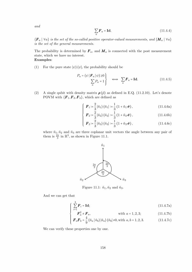
and
∑a
FFF a = Id. (11.4.4)
FFF a ∣ ∀a is the set of the so-called positive operator-valued measurements, and MMMa ∣ ∀ais the set of the general measurements.
The probability is determined by FFF a, and MMMa is connected with the post measurementstate, which we have no interest.Examples:
(1) For the pure state ∣ψ⟩ ⟨ψ∣, the probability should be
Pa = ⟨ψ ∣FFF a ∣ψ⟩≥0
∑a
Pa = 1
⎫⎪⎪⎪⎬⎪⎪⎪⎭⇐⇒ ∑
a
FFF a = Id. (11.4.5)
(2) A single qubit with density matrix ρρρ (p) as defined in E.Q. (11.2.10). Let’s denotePOVM with FFF 1,FFF 2,FFF 3, which are defined as
⎧⎪⎪⎪⎪⎪⎪⎪⎪⎪⎨⎪⎪⎪⎪⎪⎪⎪⎪⎪⎩
FFF 1 ∶=2
3∣n1⟩ ⟨n1∣ ∶=
1
3(1 + n1⋅σσσ) , (11.4.6a)
FFF 2 ∶=2
3∣n2⟩ ⟨n2∣ ∶=
1
3(1 + n2⋅σσσ) , (11.4.6b)
FFF 3 ∶=2
3∣n3⟩ ⟨n3∣ ∶=
1
3(1 + n3⋅σσσ) , (11.4.6c)
where n1, n2 and n3 are three coplanar unit vectors the angle between any pair ofthem is 2π
3 in R3, as shown in Figure 11.1.
n1
n2 n3
2π3
2π3
2π3
Figure 11.1: n1, n2 and n3.
And we can get that
3
∑i=1
FFF i = Id; (11.4.7a)⎧⎪⎪⎪⎪⎪⎪⎪⎪⎨⎪⎪⎪⎪⎪⎪⎪⎪⎩
FFF 2a ≠ FFF a, with a = 1,2,3; (11.4.7b)
FFF aFFF b =4
9⟨na ∣ nb⟩ ∣na⟩ ⟨nb∣≠0,with a, b = 1,2,3. (11.4.7c)
We can verify these properties one by one.
158

a)
3
∑i=1
FFF i = 1
3(1 + n1⋅σσσ) +
1
3(1 + n2⋅σσσ) +
1
3(1 + n3⋅σσσ)
= 1
3[3 + (n1 + n2 + n3) ⋅σσσ]
= 1
3(3 + 0)
= Id. (11.4.8)
b)
FFF aFFF a = (2
3)
2
∣na⟩ ⟨na ∣ na⟩ ⟨na∣
= (2
3)
2
∣na⟩ ∣na⟩
= 2
3FFF a. (11.4.9)
c)
FFF aFFF b = 1
9(1 + na⋅σσσ) (1 + nb⋅σσσ)
= 1
9[1 + (na + nb) ⋅σσσ + (na⋅σσσ) (nb⋅σσσ)]
= 1
9[1 + (na + nb) ⋅σσσ + na⋅nb] , (11.4.10)
thereforeFFF aFFF b ≠ 0, (11.4.11)
since FFF aFFF b vanishes iffnb = −na. (11.4.12)
11.5 More on POVM
11.5.1 Dimensional analysis
For a Hilbert space H , the number of projectors should be
#ΠΠΠn = dimH , (11.5.1)
while the number of POVM should satisfy
#FFFn ≥ dimH . (11.5.2)
11.5.2 POVM on subsystem can be viewed as projective measurementson the entire system
POVM can be viewed as projective measurement on a larger Hilbert space.‘With EEEAa
being the projective measurement on the original Hilbert space HA and FFFAa being the
POVM on the HA. There is a larger Hilbert space HA′ with HA ⊆ HA′ , such that FFFAa
are the projective measurements on HA′ .
159

11.5.3 Tensor product realization of POVM
Thm 11.5.3.1. Given one dimension non-negative POVM FFFAa on HA, there exist HB
such thatProb(a) = trAB [EEEAB
a (ρρρA⊗ρρρB)] = trA (FFFAa ρρρA) , (11.5.3)
where EEEABa are the projective measurements on HA⊗HB.
We would construct FFFAa from EEEAB
a , namely
Pa = A
ρρρA FFFAa
=
AρρρA
EEEa⊗ρρρB
B ,
(11.5.4)
where the circles mean traces.Let’s assume that ∣i⟩A = ∣j⟩A is an orthonormal basis of the Hilbert space HA, and∣µ⟩B = ∣ν⟩B is an orthonormal basis of the Hilbert space HB. Then ∣iµ⟩AB = ∣jν⟩ABis an orthonormal basis of the Hilbert space HA⊗HB.
11.5.3.1 Operator formula of FFF a
ρρρB = IIIA⊗ρρρB, and trBρρρB = trAB (IIIA⊗ρρρB) = 1, (11.5.5)
and
trA (FFFAa ρρρA) = trAB [EEEAB
a (ρρρA⊗ρρρB)]= trA trB [EEEAB
a (IIIA⊗ρρρB)]ρρρA (11.5.6)
Therefor,FFFAa = trB [EEEAB
a (IIIA⊗ρρρB)] . (11.5.7)
11.5.3.2 Matrix formalism of Fa
trA (FFF aρρρA) = ∑j
⟨j ∣FFF aρρρA ∣ j⟩
= ∑i,j
⟨j ∣FFF a ∣ i⟩ ⟨i ∣ρρρA ∣ j⟩ , (11.5.8)
trAB [EEEABa (ρρρA⊗ρρρB)] = ∑
j,νi,µ
⟨jν ∣EEEABa ∣ iµ⟩ ⟨iµ ∣ρρρA⊗ρρρB ∣ jν⟩
= ∑j,νi,µ
⟨jν ∣EEEABa ∣ iµ⟩ ⟨i ∣ρρρA ∣ j⟩ ⟨µ ∣ρρρB ∣ν⟩ (11.5.9)
Therefor, we can get that
⟨j ∣FFFAa ∣ i⟩ =∑
µ,ν
⟨jν ∣EEEABa ∣EEEAB
a ∣ iµ⟩ ⟨µ ∣ρρρB ∣ν⟩ . (11.5.10)
160

11.5.3.3 The properties of FFFAa
1) Hermitian. With E.Q.(11.5.7) and E.Q.(11.5.10), we can infer from
(EEEABa )† =EEEa and ρρρ†
B = ρρρB,
thatFFF †a = FFF a. (11.5.11)
2) Positivity, i.e. FFFAa ≥ 0. We can get the diagonal form of ρρρB, i.e.
ρρρB =∑µ
Pµ ∣µ⟩B ⟨µ∣ , with ∑µ
Pµ = 1, and 0 ≤ Pµ ≤ 1. (11.5.12)
Combine this with E.Q.(11.5.7), and we can get
A ⟨ψ ∣FFFAa ∣ψ⟩
A= A ⟨ψ ∣ trB [EEEAB
a (IIIA⊗ρρρB)] ∣ψ⟩A
= ∑µ,ν
A ⟨ψ∣B ⟨ν ∣EEEABa ∣µ⟩
B∣ψ⟩A B ⟨µ ∣ρρρB ∣ν⟩B
= ∑µ,ν
A ⟨ψ∣B ⟨ν ∣EEEABa ∣µ⟩
B∣ψ⟩A Pµδµν
= ∑µ
A ⟨ψ∣B ⟨µ ∣EEEABa ∣µ⟩
B∣ψ⟩A Pµ. (11.5.13)
Thus,
A ⟨ψ ∣FFFAa ∣ψ⟩
A≥ 0, (11.5.14)
sinceEEEABa ≥ 0, and Pµ ≥ 0.
3) Completeness.
∑a
FFFAa = ∑
a
trB [EEEABa (IIIA⊗ρρρB)]
= trB [∑a
EEEABa (IIIA⊗ρρρB)]
= trB(IIIA⊗ρρρB)= IIIA⊗trBρρρB
= IIIA. (11.5.15)
11.5.3.4 Example
We are going to talking about an example that has been discussed at the beginning ofsection 11.4. The POVM are FFFA
a ∣ a = 1,2,3, and the explicit expression should be
FFFAa = 2
3∣na⟩ ⟨na∣ , with a = 1,2,3. (11.5.16)
And the vectors na∣a = 1,2,3. are shown in Figure 11.1, from which we can concludethat
n1 + n2 + n3 = 0. (11.5.17)
161

Now, we introduce an auxiliary Hilbert space HB and the density matrix ρB on HB. Thedensity matrix of the subsystem B is
ρρρB ∶= ∣0⟩B ⟨0∣ . (11.5.18)
Which makes the density matrix of the compound Hilbert space HA⊗HB be
ρρρAB ∶= ρρρA⊗ρρρB
= ρρρA⊗ ∣0⟩B ⟨0∣ . (11.5.19)
We can also define that
∣Φa⟩AB ∶=√
2
3∣na⟩A ∣0⟩B +
√1
3∣0⟩A ∣1⟩B , with a = 1,2,3. (11.5.20)
It can easily verify that ∣Φa⟩AB ∣a = 1,2,3. makes an orthonormal basis for the compoundHilbert space HA⊗HB.
AB ⟨Φa′ ∣Φa⟩AB
=⎛⎝
√2
3A ⟨na′ ∣B ⟨0∣ +
√1
3A ⟨0∣B ⟨1∣
⎞⎠⎛⎝
√2
3∣na⟩A ∣0⟩B +
√1
3∣0⟩A ∣1⟩B
⎞⎠
= 2
3A ⟨na′ ∣ na⟩A + 1
3,
where we have the power to set
A ⟨na′ ∣ na⟩A =
⎧⎪⎪⎪⎪⎨⎪⎪⎪⎪⎩
− 1
2, if a ≠ a′;
1, if a = a′.(11.5.21)
If we define further that∣Φ0⟩AB ∶= ∣1⟩A⊗ ∣1⟩B , (11.5.22)
then we can get⟨Φa′ ∣Φa⟩ = δaa′ , ∀a, a′ ∈ 0,1,2,3 . (11.5.23)
With the orthonormal basis ∣Φa⟩AB ∣a = 0,1,2,3. , we can construct the projectors in thefollowing manner
EEEABa = ∣Φa⟩AB ⟨Φa∣
=⎛⎝
√2
3∣na⟩A ∣0⟩B +
√1
3∣0⟩A ∣1⟩B
⎞⎠⎛⎝
√2
3A ⟨na∣B ⟨0∣ +
√1
3A ⟨0∣B ⟨1∣
⎞⎠
= 2
3∣na⟩A ∣0⟩B A ⟨na∣B ⟨0∣ + 1
3∣0⟩A ∣1⟩B A ⟨0∣B ⟨1∣
+√
2
3∣na⟩A ∣0⟩B A ⟨0∣B ⟨1∣ +
√2
3∣0⟩A ∣1⟩B A ⟨na∣B ⟨0∣ ,
namely
EEEABa = 2
3∣na⟩A ⟨na∣⊗ ∣0⟩B ⟨0∣ + 1
3∣0⟩A ⟨0∣⊗ ∣1⟩B ⟨1∣
+√
2
3∣na⟩A ⟨0∣⊗ ∣0⟩B ⟨1∣ +
√2
3∣0⟩A ⟨na∣⊗ ∣1⟩B ⟨0∣ , (11.5.24)
162
for a = 1,2,3. And EEEAB0 on the other hand, is defined as
EEEAB0 ∶= ∣Φ0⟩AB ⟨Φ0∣
= ∣1⟩A ⟨1∣⊗ ∣1⟩B ⟨1∣ . (11.5.25)
Therefore,
EEEABa (IIIA⊗ρρρB)
= EEEABa (IIIA⊗ ∣0⟩B ⟨0∣)
= 2
3∣na⟩A ⟨na∣⊗ ∣0⟩B ⟨0∣ +
√2
3∣0⟩A ⟨na∣⊗ ∣1⟩B ⟨0∣ , (11.5.26)
for a = 1,2,3, andEEEABa (IIIA⊗ρρρB) = 0. (11.5.27)
Thus,
FFFAa = trB [EEEAB
a (IIIA⊗ρρρB)] = 2
3∣na⟩A ⟨na∣ , (11.5.28)
for a = 1,2,3, andFFFA
0 = 0. (11.5.29)
Therefore, the relation 11.5.7 is verified in this special case.
11.5.4 Direct-sum realization of POVM
11.5.5 POVM as quantum operation (superoperator)
11.6 Quantum operation (superoperator)
11.6.1 Definition of the superoperator
Question: What’s the evolution equation of density matrix?
y As we know, for the pure state, ∣ψ⟩, ρ = ∣ψ⟩ ⟨ψ∣, ∣ψ⟩ satisfies the Shrodinger Equation,which means it would evolve under unitary transformation, i.e.
∣ψ⟩ UUU→ UUU ∣ψ⟩ , (11.6.1)
ρρρ ∶= ∣ψ⟩ ⟨ψ∣ UUU→ UUU ∣ψ⟩ ⟨ψ∣UUU † = UUUρρρUUU †. (11.6.2)
y As for the mixed state described by ρρρ, let’s assume that
ρρρSSS→ ρρρ′ = SSS(ρρρ), (11.6.3)
where SSS is the so-called “superoperator”. We are now going to explore some prop-erties of the superoperator S.As we shall see that both ρρρ and ρρρ′ are density matrices. Therefore, SSS is a mappingbetween density matrices. We can assume that the superoperator is
• a linear mapping on density matrices, i.e.
SSS(λ1ρρρ1 + λ2ρρρ2) = λ1SSS(ρρρ1) + λ2SSS(ρρρ2), with λ1, λ2 ∈ C; (11.6.4)
163

• trace-preserving mapping (TP), namely
tr [SSS(ρρρ)] = tr(ρρρ) = 1; (11.6.5)
• positive mapping (P), i.e.SSS(ρρρ) ≥ 0. (11.6.6)
Therefore, SSS should be a linear positive trace-preserving operator.
11.6.2 The wonderful theorem
The following are equivalent.
1) SSS(ρρρ) is a CPTP mapping (Complete-Positive-trace-preserving).
⎧⎪⎪⎨⎪⎪⎩
SSS(ρρρ) ≥ 0, Positive;
(SSS⊗Id)ρρρAB ≥ 0, Complete Positive.(11.6.7)
2) The Kraus representation theorem.
Thm 11.6.2.1 (Kraus representation). A CPTP mapping SSS(ρρρ) has the operatorsum representation,
SSS(ρρρ) =∑µ
MMMµρρρMMM†µ, (11.6.8)
with the Kraus operators MMMµ satisfying
∑µ
MMM †µMMMµ = Id. (11.6.9)
3) The Stinespring representation
SSS(ρρρA) = trB [UUUAB(ρρρA⊗ ∣0⟩B ⟨0∣)UUU †AB] , (11.6.10)
or in the diagram representation
A ∶ ρρρAUUUAB
SSS(ρρρA)B ∶ ∣0⟩B ⟨0∣
.
(11.6.11)
The symbol stands for the recycle bin, which means that the correspondingoutput qubit is within our interest.Math tool: Function Analysis.
4) The Choi-Jamiolkowski representation
164
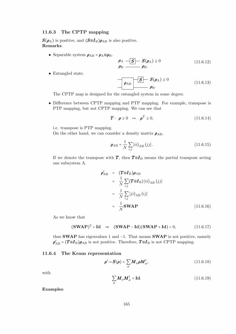
11.6.3 The CPTP mapping
SSS(ρρρA) is positive, and (SSS⊗IIIB)ρρρAB is also positive.Remarks:
• Separable system ρρρAB = ρρρA⊗ρρρB.
ρρρA SSS SSS(ρρρA) ≥ 0ρρρB ρρρB.
(11.6.12)
• Entangled state.
ρρρABSSS SSS(ρρρA) ≥ 0
ρρρB.(11.6.13)
The CPTP map is designed for the entangled system in some degree.
• Difference between CPTP mapping and PTP mapping. For example, transpose isPTP mapping, but not CPTP mapping. We can see that
TTT ∶ ρρρ ≥ 0 ↦ ρρρT ≥ 0, (11.6.14)
i.e. transpose is PTP mapping.On the other hand, we can consider a density matrix ρρρAB,
ρρρAB = 1
N∑i,j
∣ii⟩AB ⟨jj∣ . (11.6.15)
If we denote the transpose with TTT , then TTT⊗IIIB means the partial transpose actingone subsystem A.
ρρρ′AB = (TTT⊗IIIB)ρρρAB
= 1
N∑i,j
(TTT⊗IIIB) ∣ii⟩AB ⟨jj∣
= 1
N∑i,j
∣ji⟩AB ⟨ij∣
= 1
NSWAP (11.6.16)
As we know that
(SWAP)2 = Id ⇒ (SWAP − Id)(SWAP + Id) = 0, (11.6.17)
thus SWAP has eigenvalues 1 and −1. That means SWAP is not positive, namelyρρρ′AB = (TTT⊗IIIB)ρρρAB is not positive. Therefore, TTT⊗IIIB is not CPTP mapping.
11.6.4 The Kraus representation
ρρρ′ ∶=SSS(ρρρ) =∑µ
MMMµρρρMMM†µ, (11.6.18)
with
∑µ
MMMµMMM†µ = Id. (11.6.19)
Examples:
165

(i) Unitary evolution of closed system,
ρρρ ↦ UUUρρρUUU †, (11.6.20)
with ⎧⎪⎪⎨⎪⎪⎩
MMM1 = UUU, MMM †1 = UUU
†;
MMM2 = 0, MMM †2 = 0.
(11.6.21)
It can be easily verified that
MMM †1MMM1 +MMM †
2MMM2 = Id. (11.6.22)
(ii) Projective measurement.
ΠΠΠn = ∣n⟩ ⟨n∣ , ∑n
ΠΠΠ†nΠΠΠn = Id. (11.6.23)
ρρρ ∶= ∣ψ⟩ ⟨ψ∣ΠΠΠnÐ→ ρρρ′ = SSS(ρρρ) =∑
n
ΠΠΠnρρρΠΠΠ†n. (11.6.24)
(iii) POVM with one-dimensional operators FFF a.
ρρρ ↦ ρρρ′ =∑a
√FFF aρρρ
√FFF a, with FFF a ≥ 0, and ∑
a
FFF a = 1. (11.6.25)
11.6.5 The Stinespring representation
A ∶ ρρρAUUUAB
SSS(ρρρA)B ∶ ∣0⟩B ⟨0∣
.
(11.6.26)
The Stinespring representation is actually equivalent to Kraus representation.
ρρρAB ∶=ρρρA⊗ ∣0⟩B ⟨0∣ ↦ ρρρ′AB ∶=UUUABρρρABUUU†AB, (11.6.27)
i.e.
ρρρ′A = trBρρρ′AB
= trB (UUUABρρρABUUU†AB)
= ∑µ
B ⟨µ∣UUUABρρρABUUU†AB ∣µ⟩B
= ∑µ
B ⟨µ∣UUUAB(ρρρA⊗ ∣0⟩B ⟨0∣ )UUU †AB ∣µ⟩B
= ∑µ
B ⟨µ∣UUUAB ∣0⟩B (ρρρA)B ⟨0∣U †AB ∣µ⟩B . (11.6.28)
We can denote that
MMMµ = B ⟨µ∣UUUAB ∣0⟩B , MMM †µ = B ⟨0∣UUU †
AB ∣µ⟩B , (11.6.29)
then
∑µ
MMM †µMMMµ = ∑
µB ⟨0∣UUU †
AB ∣µ⟩B ⟨µ∣UUUAB ∣0⟩B
= B ⟨0∣UUU †ABUUUAB ∣0⟩B
= IIIA. (11.6.30)
166

11.6.6 Remarks on quantum operation
11.7 Quantum channel
Example for Quantum Operation:ρρρ SSS ρρρ′ = SSS(ρρρ), (11.7.1)
where the superoperator SSS is a channel.
11.7.1 The bit-flip channel
The Quantum Bit-flip:
∣0⟩ XXX↦ ∣1⟩ , ∣1⟩ XXX↦ ∣0⟩ , with XXX = σσσx. (11.7.2)
This means Quantum error-model:
∣1⟩
∣0⟩
∣0⟩
p
1 − p,
∣0⟩
∣1⟩
∣1⟩
p
1 − p, (11.7.3)
where p is the error-probability, 0 ≤ p ≤ 1, namely
SSS(∣0⟩ ⟨0∣) = (1 − p) ∣0⟩ ⟨0∣ + p ∣1⟩ ⟨1∣ ; (11.7.4a)
SSS(∣1⟩ ⟨1∣) = p ∣0⟩ ⟨0∣ + (1 − p) ∣1⟩ ⟨1∣ . (11.7.4b)
Thereforeρρρ ↦ ρρρ′ ∶=SSS(ρρρ) = (1 − p)ρρρ + pXXXρρρXXX (11.7.5)
We can then get the Kraus operators
⎧⎪⎪⎪⎪⎪⎪⎨⎪⎪⎪⎪⎪⎪⎩
MMM0 =√
1 − pIII2 =√
1 − p(1 00 1
) ;
MMM1 =√pXXX = √
p(0 11 0
) .(11.7.6)
And we can verify that
MMM †0MMM0 +MMM †
1MMM1 = (1 − p)(III2)2 + pXXX2
= (1 − p)III2 + pIII2
= III2. (11.7.7)
1) Unitary Representation (Stine Spring representation).
A ∶ ∣ψ⟩AUUUAB
SSS (∣ψ⟩A ⟨ψ∣)B ∶ ∣0⟩B
,
(11.7.8)
where
UUUAB (∣ψ⟩A⊗ ∣0⟩B) ∶= (MMM0⊗III2 + iMMM1⊗XXX) ∣ψ⟩A⊗ ∣0⟩B
=√
1 − p ∣ψ⟩A⊗ ∣0⟩B + i√pXXX ∣ψ⟩A⊗ ∣1⟩B (11.7.9)
167

Then,
ρρρ′A
= SSS(ρρρA)= trB (UUUAB( ∣ψ⟩A ⟨ψ∣⊗ ∣0⟩B ⟨0∣ )UUU †
AB)
= trB[(√
1 − p ∣ψ⟩A⊗ ∣0⟩B + i√pXXX ∣ψ⟩A⊗ ∣1⟩B)
(√
1 − pA ⟨ψ∣⊗B ⟨0∣ − i√pA ⟨ψ∣XXX⊗B ⟨1∣)]
= trB[(1 − p) ∣ψ⟩A ⟨ψ∣⊗ ∣0⟩B ⟨0∣ + pXXX ∣ψ⟩A ⟨ψ∣XXX⊗ ∣1⟩B ⟨1∣)]
+i√p(1 − p)trB( − ∣ψ⟩A ⟨ψ∣XXX⊗ ∣0⟩B ⟨1∣ +XXX ∣ψ⟩A ⟨ψ∣⊗ ∣1⟩B ⟨0∣ )
= (1 − p) ∣ψ⟩A ⟨ψ∣ + pXXX ∣ψ⟩A ⟨ψ∣XXX, (11.7.10)
and
UUU †ABUUUAB = (MMM0⊗III2 + iMMM1⊗XXX)†(MMM0⊗III2 + iMMM1⊗XXX)
= MMM †0MMM0⊗III2 +MMM †
1MMM1⊗XXX2 − i(MMM †1MMM0⊗XXX −MMM †
0MMM1⊗XXX)
= (MMM †0MMM0 +MMM †
1MMM1)⊗III2 − i(MMM1MMM0⊗XXX −MMM0MMM1⊗XXX)= III2⊗III2 − i(MMM1MMM0⊗XXX −MMM1MMM0⊗XXX)= III4, (11.7.11)
where we have used the fact that for this special case the Kraus operators satisfies
⎧⎪⎪⎨⎪⎪⎩
MMM †0 =MMM0, (11.7.12a)
MMM †1 =MMM1, (11.7.12b)
as is shown in E.Q.(11.7.6). Thus, we can also verify in a similar manner that
UUUABUUU†AB = III4. (11.7.13)
Therefore,UUUAB ∶=MMM0⊗III2 + iMMM1⊗XXX (11.7.14)
is unitary.
2) The Bloch sphere representation.
ρρρ = 1
2(Id + p3ZZZ) (11.7.15)
with∣p3∣ ≤ 1, p = p3e3, (11.7.16)
andZZZ = σσσ3. (11.7.17)
Therefore,
SSS(ρρρ) = (1 − p)ρρρ + pXXXρρρXXX
= 1
2(Id + p′3ZZZ), (11.7.18)
168

withp′3 ∶= (1 − 2p)p3, (11.7.19)
since
(1 − p)ρρρ + pXXXρρρXXX = 1 − p2
(Id + p3ZZZ) + p2XXX (Id + p3ZZZ)XXX
= 1 − p2
(Id + p3ZZZ) + p2(Id − p3ZZZ)
= 1
2[Id + (1 − 2p)p3ZZZ] . (11.7.20)
Because ∣1 − 2p∣ ≤ 1, we may conclude here that the inflation is not permitted here inQuantum Mechanics.
11.7.2 The phase-flip channel
Next, we are going to discuss the Phase-flip error, which exists in Quantum Mechanicsand there is no Classical analogy.Phase-flip error:
∣0⟩ → ∣0⟩ , ∣1⟩ → − ∣1⟩ . (11.7.21)
Therefore, the Phase-flip channel should be of the form of
SSS(ρρρ) = (1 − p)ρρρ + pZZZρρρZZZ. (11.7.22)
And we can define the bit-phase-flip error as
SSS(ρρρ) = (1 − p)ρρρ + pYYY ρρρYYY , with YYY = σσσy. (11.7.23)
11.7.3 Depolarizing channel
Depolarizing means that
Polarization(ρρρ) ↦ Non − polarization(ρρρ). (11.7.24)
AndSSS(ρρρ) = (1 − p)ρρρ + p
3(XXXρρρXXX +YYY ρρρYYY +ZZZρρρZZZ) , (11.7.25)
and the Kraus operators
MMM0 ∶=√
1 − pIII2, MMM1 ∶=√p
3XXX, MMM2 ∶=
√p
3YYY , MMM3 ∶=
√p
3ZZZ. (11.7.26)
We can verify that
3
∑i=0
MMM †iMMM i = MMM †
0MMM0 +MMM †1MMM1 +MMM †
2MMM2 +MMM †3MMM3
= (1 − p)III2 +p
3III2 +
p
3III2 +
p
3III2
= III2.
The Bloch Sphere representation.
ρρρ = 1
2(Id + p⋅σσσ) , with ∥p∥ ≤ 1 and p ∈ R3. (11.7.27)
169

Therefore,
SSS(ρρρ) = 1
2SSS(1 + p⋅σσσ)
= 1
2[SSS(III2) +SSS(p⋅σσσ)]
= 1
2[III2 + (1 − p)p⋅σσσ + p
3(XXXp⋅σσσXXX +YYY p⋅σσσYYY +ZZZp⋅σσσZZZ)]
= 1
2III2 + (1 − p)p⋅σσσ + p
3[(p1 − p1 − p1)XXX + (−p2 + p2 − p2)YYY + (−p3 − p3 + p3)ZZZ]
= 1
2[III2 + (1 − p)p⋅σσσ − 2p
3p⋅σσσ]
= 1
2(III2 + p′⋅σσσ) , (11.7.28)
with
p′ ∶= (1 − 4p
3) p. (11.7.29)
11.7.4 The phase-damping channel
ρρρSSS↦ SSS(ρρρ) =
2
∑i=0
MMM iρρρMMM†i , (11.7.30)
withMMM0 ∶=
√1 − pIII2, MMM1 ∶=
√p ∣0⟩ ⟨0∣ , MMM2 ∶=
√p ∣1⟩ ⟨1∣ . (11.7.31)
Therefore, with the matrix expression of the density matrix ρρρ,
ρρρ ∶= (ρ00 ρ01
ρ10 ρ11) , (11.7.32)
we can get
SSS(ρρρ) = (1 − p)ρρρ + p(ρ00 00 ρ11
)
= ( ρ00 (1 − p)ρ01
(1 − p)ρ10 ρ11) . (11.7.33)
As we shall see that from ρρρ to SSS(ρρρ),
• the diagonal terms are unchanged;
• the non-diagonal terms decay with the factor (1 − p).
Therefore, we can get that
SSSn(ρρρ) ∶= SSS0SSS0⋯SSS0´¹¹¹¹¹¹¹¹¹¹¹¹¹¹¹¹¹¸¹¹¹¹¹¹¹¹¹¹¹¹¹¹¹¹¹¹¶
n
ρρρ
= ( ρ00 (1 − p)nρ01
(1 − p)nρ10 ρ11) . (11.7.34)
We can conclude immediately that with n → ∞, then (1−p)n → 0, there we can get finallyget
SSSn(ρρρ) n→∞Ð→ (ρ00 00 ρ11
) , (11.7.35)
i.e. the non-diagonal terms vanish.
170

11.7.5 The amplitude-damping channel
ρρρSSS↦ SSS(ρρρ) =MMM0ρρρMMM
†0 +MMM1ρρρMMM
†1, (11.7.36)
with
MMM0 ∶= (1 00
√1 − p) , MMM1 = (0
√p
0 0) . (11.7.37)
We can verify that
MMM †0MMM0 +MMM †
1MMM0 = (1 00
√1 − p)(1 0
0√
1 − p) + ( 0 0√p 0
)(0√p
0 0)
= (1 00 1 − p) + (0 0
0 p)
= (1 00 1
)
= III2. (11.7.38)
Therefore,
SSS(ρρρ) = (1 00
√1 − p)(ρ00 ρ01
ρ10 ρ11)(1 0
0√
1 − p)
+(0√p
0 0)(ρ00 ρ01
ρ10 ρ11)( 0 0√
p 0)
= ( ρ00√
1 − pρ01√1 − pρ10 (1 − p)ρ11
) + (pρ11 00 0
)
= (ρ00 + pρ11√
1 − pρ01√1 − pρ10 (1 − p)ρ11
) , (11.7.39)
i.e.
SSS(ρρρ) = (ρ00 + ρ11 − (1 − p)ρ11√
1 − pρ01√1 − pρ10 (1 − p)ρ11
) . (11.7.40)
Thus
SSSn(ρρρ) = (ρ00 + ρ11 − (1 − p)nρ11 (1 − p)n/2ρ01
(1 − p)n/2ρ10 (1 − p)nρ11) , (11.7.41)
with n→∞, (1 − p)n→0, i.e.
SSSn(ρρρ) n→∞Ð→ (ρ00 + ρ11 00 0
) . (11.7.42)
Example: Ifρρρ ∶= ∣a∣2 ∣0⟩ ⟨0∣ + ∣b∣2 ∣1⟩ ⟨1∣ , with ∣a∣2 + ∣b∣2 = 1, (11.7.43)
we can get
SSSn(ρρρ) n→∞Ð→ (∣a∣2 + ∣b∣2 0
0 0) = (1 0
0 0) = ∣0⟩ ⟨0∣ . (11.7.44)
Therefore, we can get the pure state ∣0⟩ ⟨0∣ from the mixed state ρρρ = ∣a∣2 ∣0⟩ ⟨0∣ + ∣b∣2 ∣1⟩ ⟨1∣.
171

11.8 The master equation
The master Equation is also called Lindblud’s Equation.In general, Quantum Operation, CPTP mapping.In special cases, Markovin process:
tm−1 tm tm+1 , (11.8.1)
where state at time ti+1 only depends on state at time ti. Therefor, in Makovin process,ρρρA(t + dt) depends only on ρρρA(t). From Figure 11.2 we can see that, we have three time
open system A with ∆tA
observer ∆tOenvironment ∆tE
interactio
n interaction
Figure 11.2: Three time scale
scales, i.e. ∆tA,∆tO and ∆tE. In Markovin process, we have
∆tA ≫ ∆tO ≫ ∆tE, (11.8.2)
which means that for the observer, the physical system is changing very slowly while theenvironment is changing very fast. This ensures that ρρρA(t + dt) depends on ρρρA(t).
1 First-order approximation.
ρρρ(dt) = ρρρ(0) +O(dt) = ρρρ(0) + dρρρ(0) (11.8.3)
2 Kraus representation.
ρρρ(dt) = SSS (ρρρ(0)) =∑µ
MMMµ(dt)ρρρ(0)MMM †µ(dt), (11.8.4)
with
∑µ
MMM †µ(dt)MMMµ(dt) = Id.
3 Assume
MMM0 = Id + (−iHHH +KKK)dt, with HHH† =HHH,KKK† =KKK; (11.8.5a)
MMMν = LLLν√
dt, with ν = 1,2,3, . . .. (11.8.5b)
4
ρρρ(0)+dρρρ(0) = [Id + (−iHHH +KKK)dt]ρρρ(0) [Id + (iHHH +KKK)dt]+∑ν
LLL†kρρρ(0)LLLkdt, (11.8.6)
thendρρρ = (−iHHH +KKK)ρρρdt + ρρρ(iHHH +KKK)dt +∑
ν=1
LLL†kρρρLLLkdt, (11.8.7)
172

i.e.dρρρ
dt= 1
i[HHH,ρρρ] + KKK,ρρρ +∑
ν
LLL†kρρρLLLk. (11.8.8)
With
∑µ
MMM †µMMMµ = Id, (11.8.9)
we infer that(−iHHH +KKK) + (iHHH +KKK) +∑
ν
LLL†νLLLν = 0, (11.8.10)
i.e.
KKK = −1
2∑ν
LLL†νLLLν . (11.8.11)
Hence, we can obtain
dρρρ
dt= 1
i[HHH,ρρρ] +∑
ν
(LLL†νρρρLLLν −
1
2LLL†
νLLLν ,ρρρ) . (11.8.12)
For the special case of KKK = 0 and LLLν = 0, ν = 1,2,3, . . ., we can get
dρρρ
dt= 1
i[HHH,ρρρ], (11.8.13)
which is the case of the closed system.
173
Chapter 12
Notes on Finite Group Theory
174

Chapter 13
Notes on Stabilizer Formalism ofQuantum Error Correction Codes
175

Part V
Selected Topics
176

Chapter 14
Entanglement Measures andEntropy: Bi-Partite System
The main problem is that we do not understand fully what entanglement is.
—Horodecki
Then the usefulness of entanglement emerges because it allows us to overcomea particular constraint that will be the LOCC constraint.
—Plenio and Virmani
It is the constraint to LOCC operations that entanglement to the status of aresource.
—Plenio and Virmani
We will simply accept the non-uniqueness of entanglement measures as anexpression of the fact that they correspond to different operational tasks underwhich different forms of entanglement may have different degree of usefulness.
—Plenio and Virmani
Reference:
[Preskill] New Chapter 4: Quantum entanglement;
177
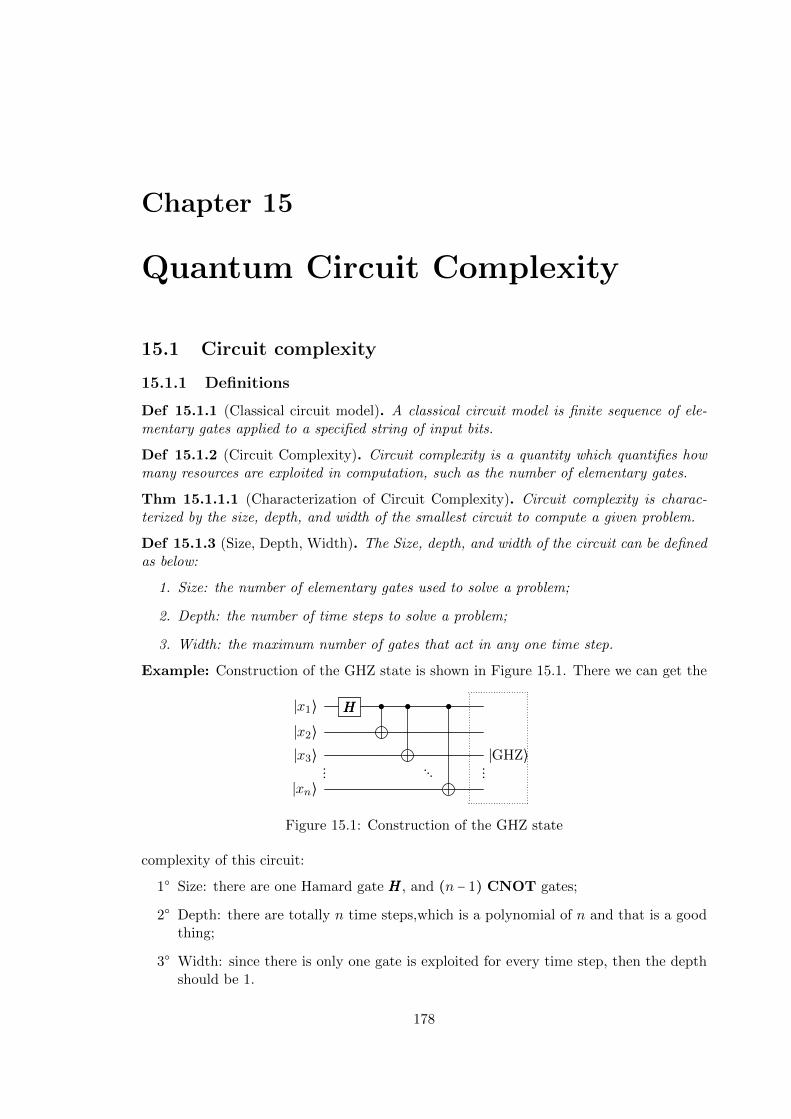
Chapter 15
Quantum Circuit Complexity
15.1 Circuit complexity
15.1.1 Definitions
Def 15.1.1 (Classical circuit model). A classical circuit model is finite sequence of ele-mentary gates applied to a specified string of input bits.
Def 15.1.2 (Circuit Complexity). Circuit complexity is a quantity which quantifies howmany resources are exploited in computation, such as the number of elementary gates.
Thm 15.1.1.1 (Characterization of Circuit Complexity). Circuit complexity is charac-terized by the size, depth, and width of the smallest circuit to compute a given problem.
Def 15.1.3 (Size, Depth, Width). The Size, depth, and width of the circuit can be definedas below:
1. Size: the number of elementary gates used to solve a problem;
2. Depth: the number of time steps to solve a problem;
3. Width: the maximum number of gates that act in any one time step.
Example: Construction of the GHZ state is shown in Figure 15.1. There we can get the
∣x1⟩ HHH
∣x2⟩∣x3⟩ ∣GHZ⟩
⋮ ⋱ ⋮∣xn⟩
Figure 15.1: Construction of the GHZ state
complexity of this circuit:
1 Size: there are one Hamard gate HHH, and (n − 1) CNOT gates;
2 Depth: there are totally n time steps,which is a polynomial of n and that is a goodthing;
3 Width: since there is only one gate is exploited for every time step, then the depthshould be 1.
178

15.1.2 Complexity class
We can classify the circuit into different categories according to the size the circuit:
size ∝ poly(n) excellent,
size ∝ Exp(n) the worst case.
Def 15.1.4 (Decision problem). A decision problem is a “yes” or “no” problem.
Def 15.1.5 (P-problem).
P-problem = decision problems which can be solved by polynomial size circuit family.
Def 15.1.6 (NP-problem).
NP-problem = decision problems which can be verified by polynomial size circuit family.
Note: verifying a problem is very different from solving a problem. For example, it wouldbe very difficult to work out a password, but with a password in hand, it would be veryeasy to verify if it works.
Question: What’s the relation between N-problem and NP-problem? It is widelybelieved, but not solved, that these two categories of problems is not equivalent toeach other. But, how can we prove or falsify that kind of consensus?
Thm 15.1.2.1 (Cock’s theorem(1971)). Every problem in NP is polynomially reducibleto NP-Completeness (NPC) problem.
Some relations between the different types of problems expressed in diagram formalismshown in Figure 15.2
NPCNPI
PNP
Decision problems
(a)
P CO-NPNP
NPC
Decision problems
(b)
Figure 15.2: Decision problem, NP, NPC, NPI and P
To be clarified in the future (2015).
15.1.3 Quantum complexity
There are two kinds of classical circuit, namely the deterministic circuits and the proba-bilistic circuit with probabilistic gates:
Classical Circuitdeterministic circuits,
probabilistic circuits with probabilistic gates,
Probabilistic gatesAND with probability ε,
OR with probability 1 − ε,e.g. simulation Monto Carlo Annealing. Classical circuit model is described by Bounded-error Probabilistic Polynomial size (BPP) problem. Quantum circuit, on the other hand,is described by Bounded-error Quantum Probabilistic Polynomial size (BQP) problem.
179

15.1.4 Accuracy
For the exact Quantum Computer, we need infinite number of quantum gates. But, thatis impossible to realize in practice. For practical consideration, we would turn to FiniteQuantum Approximately Universal Gate set, with which we can get the result in arbitraryaccuracy. So the precision is an important topics.
180

Chapter 16
Integrable Quantum Computation
Interested readers are invited to refer to two documents on the same homepage: the one isthe published paper with the title of “Integrable Quantum Computation”; and the otherone is the associated .ppt file of interpreting the published one.
181