lecture notes for math 417-517 multivariable...
TRANSCRIPT
Lecture notes for Math 417-517Multivariable Calculus
J. DimockDept. of Mathematics
SUNY at BuffaloBuffalo, NY 14260
December 4, 2012
Contents
1 multivariable calculus 31.1 vectors . . . . . . . . . . . . . . . . . . . . . . . . . . . . . . . . . . . . 31.2 functions of several variables . . . . . . . . . . . . . . . . . . . . . . . . 51.3 limits . . . . . . . . . . . . . . . . . . . . . . . . . . . . . . . . . . . . . 61.4 partial derivatives . . . . . . . . . . . . . . . . . . . . . . . . . . . . . . 61.5 derivatives . . . . . . . . . . . . . . . . . . . . . . . . . . . . . . . . . . 81.6 the chain rule . . . . . . . . . . . . . . . . . . . . . . . . . . . . . . . . 111.7 implicit function theorem -I . . . . . . . . . . . . . . . . . . . . . . . . 141.8 implicit function theorem -II . . . . . . . . . . . . . . . . . . . . . . . . 181.9 inverse functions . . . . . . . . . . . . . . . . . . . . . . . . . . . . . . 211.10 inverse function theorem . . . . . . . . . . . . . . . . . . . . . . . . . . 231.11 maxima and minima . . . . . . . . . . . . . . . . . . . . . . . . . . . . 261.12 differentiation under the integral sign . . . . . . . . . . . . . . . . . . . 291.13 Leibniz’ rule . . . . . . . . . . . . . . . . . . . . . . . . . . . . . . . . . 301.14 calculus of variations . . . . . . . . . . . . . . . . . . . . . . . . . . . . 32
2 vector calculus 362.1 vectors . . . . . . . . . . . . . . . . . . . . . . . . . . . . . . . . . . . . 362.2 vector-valued functions . . . . . . . . . . . . . . . . . . . . . . . . . . . 402.3 other coordinate systems . . . . . . . . . . . . . . . . . . . . . . . . . . 432.4 line integrals . . . . . . . . . . . . . . . . . . . . . . . . . . . . . . . . . 482.5 double integrals . . . . . . . . . . . . . . . . . . . . . . . . . . . . . . . 512.6 triple integrals . . . . . . . . . . . . . . . . . . . . . . . . . . . . . . . . 552.7 parametrized surfaces . . . . . . . . . . . . . . . . . . . . . . . . . . . . 57
1
2.8 surface area . . . . . . . . . . . . . . . . . . . . . . . . . . . . . . . . . 602.9 surface integrals . . . . . . . . . . . . . . . . . . . . . . . . . . . . . . . 622.10 change of variables in R2 . . . . . . . . . . . . . . . . . . . . . . . . . . 642.11 change of variables in R3 . . . . . . . . . . . . . . . . . . . . . . . . . 672.12 derivatives in R3 . . . . . . . . . . . . . . . . . . . . . . . . . . . . . . 702.13 gradient . . . . . . . . . . . . . . . . . . . . . . . . . . . . . . . . . . . 722.14 divergence theorem . . . . . . . . . . . . . . . . . . . . . . . . . . . . . 742.15 applications . . . . . . . . . . . . . . . . . . . . . . . . . . . . . . . . . 782.16 more line integrals . . . . . . . . . . . . . . . . . . . . . . . . . . . . . 832.17 Stoke’s theorem . . . . . . . . . . . . . . . . . . . . . . . . . . . . . . . 872.18 still more line integrals . . . . . . . . . . . . . . . . . . . . . . . . . . . 922.19 more applications . . . . . . . . . . . . . . . . . . . . . . . . . . . . . . 972.20 general coordinate systems . . . . . . . . . . . . . . . . . . . . . . . . . 99
3 complex variables 1063.1 complex numbers . . . . . . . . . . . . . . . . . . . . . . . . . . . . . . 1063.2 definitions and properties . . . . . . . . . . . . . . . . . . . . . . . . . . 1073.3 polar form . . . . . . . . . . . . . . . . . . . . . . . . . . . . . . . . . . 1103.4 functions . . . . . . . . . . . . . . . . . . . . . . . . . . . . . . . . . . . 1113.5 special functions . . . . . . . . . . . . . . . . . . . . . . . . . . . . . . . 1133.6 derivatives . . . . . . . . . . . . . . . . . . . . . . . . . . . . . . . . . . 1153.7 Cauchy-Riemann equations . . . . . . . . . . . . . . . . . . . . . . . . . 1183.8 analyticity . . . . . . . . . . . . . . . . . . . . . . . . . . . . . . . . . . 1203.9 complex line integrals . . . . . . . . . . . . . . . . . . . . . . . . . . . . 1213.10 properties of line integrals . . . . . . . . . . . . . . . . . . . . . . . . . 1233.11 Cauchy’s theorem . . . . . . . . . . . . . . . . . . . . . . . . . . . . . . 1253.12 Cauchy integral formula . . . . . . . . . . . . . . . . . . . . . . . . . . 1273.13 higher derivatives . . . . . . . . . . . . . . . . . . . . . . . . . . . . . . 1313.14 Cauchy inequalities . . . . . . . . . . . . . . . . . . . . . . . . . . . . . 1323.15 real integrals . . . . . . . . . . . . . . . . . . . . . . . . . . . . . . . . . 1343.16 Fourier and Laplace transforms . . . . . . . . . . . . . . . . . . . . . . 137
2

1 multivariable calculus
1.1 vectors
We start with some definitions. A real number x is positive, zero, or negative and isrational or irrational. We denote
R = set of all real numbers x (1)
The real numbers label the points on a line once we pick an origin and a unit of length.Real numbers are also called scalars
Next defineR2 = all pairs of real numbers x = (x1, x2) (2)
The elements of R2 label points in the plane once we pick an origin and a pair oforthogonal axes. Elements of R2 are also called (2-dimensional) vectors and can berepresented by arrows from the origin to the point represented.
Next defineR3 = all triples of real numbers x = (x1, x2, x3) (3)
The elements of R3 label points in space once we pick an origin and three orthogonalaxes. Elements of R3 are (3-dimensional) vectors. Especially for R3 one might em-phasize that x is a vector by writing it in bold face x = (x1, x2, x3) or with an arrow~x = (x1, x2, x3) but we refrain from doing this for the time being.
Generalizing still further we define
Rn = all n-tuples of real numbers x = (x1, x2, . . . , xn) (4)
The elements of Rn are the points in n-dimensional space and are also called (n-dimensional) vectors
Given a vector x = (x1, . . . , xn) in Rn and a scalar α ∈ R the product is the vector
αx = (αx1, . . . , αxn) (5)
Another vector y = (y1, . . . , yn) can to added to x to give a vector
x+ y = (x1 + y1, . . . , xn + yn) (6)
Because elements of Rn can be multiplied by a scalar and added it is called a vectorspace. We can also subtract vectors defining x− y = x+ (−1)y and then
x− y = (x1 − y1, . . . , xn − yn) (7)
For two or three dimensional vectors these operations have a geometric interpreta-tion. αx is a vector in the same direction as x (opposite direction if α < 0) with length
3

Figure 1: vector operations
increased by |α|. The vector x + y can be found by completing a parallelogram withsides x, y and taking the diagonal, or by putting the tail of y on the head of x anddrawing the arrow from the tail of x to the head of y. The vector x − y is found bydrawing x+ (−1)y. Alternatively if the tail of x− y put a the head of y then the arrowgoes from the head of y to the head of x. See figure 1.
A vector x = (x1, . . . , xn) has a length which is
|x| = length of x =√x2
1 + · · ·+ x2n (8)
Since x−y goes from the point y to the point x, the length of this vector is the distancebetween the points:
|x− y| = distance between x and y =√
(x1 − y1)2 + · · ·+ (xn − yn)2 (9)
One can also form the dot product of vectors x, y in Rn. The result is a scalar givenby
x · y = x1y1 + x2y2 + · · ·+ xnyn (10)
Then we havex · x = |x|2 (11)
4
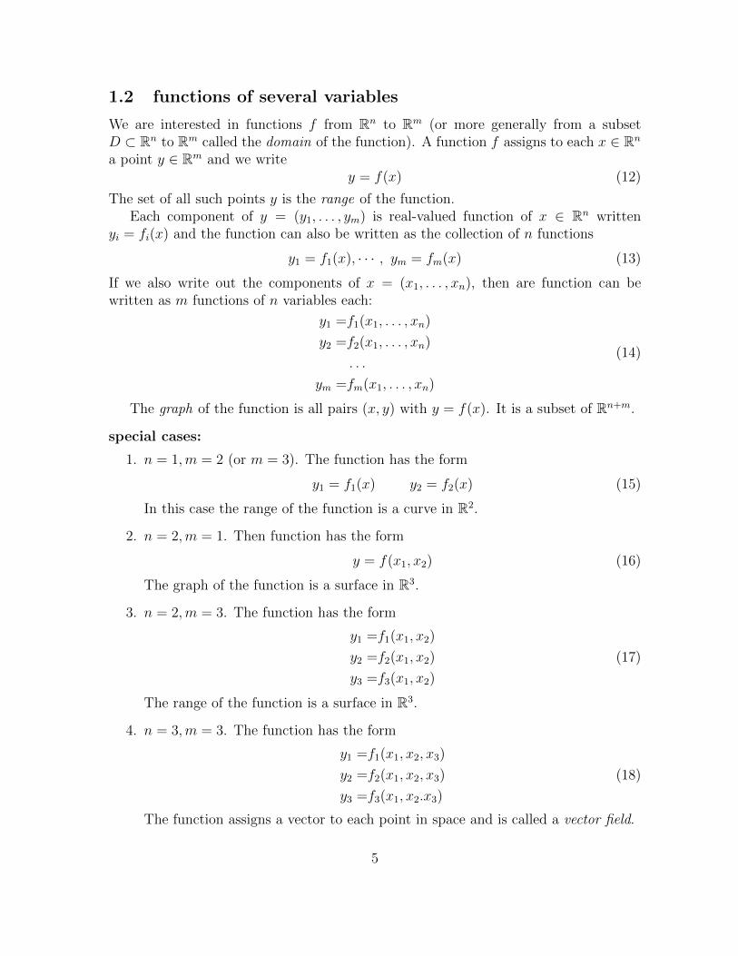
1.2 functions of several variables
We are interested in functions f from Rn to Rm (or more generally from a subsetD ⊂ Rn to Rm called the domain of the function). A function f assigns to each x ∈ Rn
a point y ∈ Rm and we writey = f(x) (12)
The set of all such points y is the range of the function.Each component of y = (y1, . . . , ym) is real-valued function of x ∈ Rn written
yi = fi(x) and the function can also be written as the collection of n functions
y1 = f1(x), · · · , ym = fm(x) (13)
If we also write out the components of x = (x1, . . . , xn), then are function can bewritten as m functions of n variables each:
y1 =f1(x1, . . . , xn)
y2 =f2(x1, . . . , xn)
. . .
ym =fm(x1, . . . , xn)
(14)
The graph of the function is all pairs (x, y) with y = f(x). It is a subset of Rn+m.
special cases:
1. n = 1,m = 2 (or m = 3). The function has the form
y1 = f1(x) y2 = f2(x) (15)
In this case the range of the function is a curve in R2.
2. n = 2,m = 1. Then function has the form
y = f(x1, x2) (16)
The graph of the function is a surface in R3.
3. n = 2,m = 3. The function has the form
y1 =f1(x1, x2)
y2 =f2(x1, x2)
y3 =f3(x1, x2)
(17)
The range of the function is a surface in R3.
4. n = 3,m = 3. The function has the form
y1 =f1(x1, x2, x3)
y2 =f2(x1, x2, x3)
y3 =f3(x1, x2.x3)
(18)
The function assigns a vector to each point in space and is called a vector field.
5
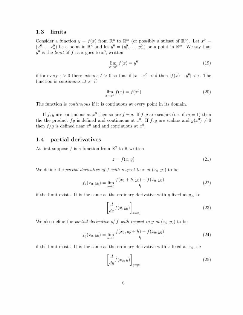
1.3 limits
Consider a function y = f(x) from Rn to Rm (or possibly a subset of Rn). Let x0 =(x0
1, . . . x0n) be a point in Rn and let y0 = (y0
1, . . . , y0m) be a point in Rm. We say that
y0 is the limit of f as x goes to x0, written
limx→x0
f(x) = y0 (19)
if for every ε > 0 there exists a δ > 0 so that if |x− x0| < δ then |f(x)− y0| < ε. Thefunction is continuous at x0 if
limx→x0
f(x) = f(x0) (20)
The function is continuous if it is continuous at every point in its domain.
If f, g are continuous at x0 then so are f ± g. If f, g are scalars (i.e. if m = 1) thenthe the product fg is defined and continuous at x0. If f, g are scalars and g(x0) 6= 0then f/g is defined near x0 and and continuous at x0.
1.4 partial derivatives
At first suppose f is a function from R2 to R written
z = f(x, y) (21)
We define the partial derivative of f with respect to x at (x0, y0) to be
fx(x0, y0) = limh→0
f(x0 + h, y0)− f(x0, y0)
h(22)
if the limit exists. It is the same as the ordinary derivative with y fixed at y0, i.e[d
dxf(x, y0)
]x=x0
(23)
We also define the partial derivative of f with respect to y at (x0, y0) to be
fy(x0, y0) = limh→0
f(x0, y0 + h)− f(x0, y0)
h(24)
if the limit exists. It is the same as the ordinary derivative with x fixed at x0, i.e[d
dyf(x0, y)
]y=y0
(25)
6

We also use the notation
fx =∂z
∂x
(or
∂f
∂xor zx
)fy =
∂z
∂y
(or
∂f
∂yor zy
) (26)
If we let (x0, y0) vary the partial derivatives are also functions and we can takesecond partial derivatives like
(fx)x ≡ fxx also written∂
∂x
(∂z
∂x
)=∂2z
∂x2(27)
The four second partial derivatives are
fxx =∂2z
∂x2fxy =
∂2z
∂y∂x
fyx =∂2z
∂x∂yfyy =
∂2z
∂y2
(28)
Usually fxy = fyx for we have
Theorem 1 If fx, fy, fxy, fyx exist and are continuous near (x0, y0) (i.e in a little disccentered on (x0, y0) ) then
fxy(x0, y0) = fyx(x0, y0) (29)
Example: Consider f(x, y) = 3x2y + 4xy3. Then
fx = 6xy + 4y3 fy = 3x2 + 12xy2
fxy = 6x+ 12y2 fyx = 6x+ 12y2 (30)
We also have partial derivatives for a function f from Rn to R written y = f(x1, . . . xn).The partial derivative with respect to xi at (x0
1, . . . x0n) is
fxi(x01, . . . x
0n) = lim
h→0
f(x01, . . . , x
0i + h, . . . , x0
n)− f(x01, . . . x
0n)
h(31)
It is also written
fxi =∂y
∂xi(32)
7
1.5 derivatives
A function z = f(x, y) is said to be differentiable at (x0, y0) if it can be well-approximatedby a linear function near that point. This means there should be constants a, b suchthat
f(x, y) = f(x0, y0) + a(x− x0) + b(y − y0) + ε(x, y) (33)
where the error term ε(x, y) is continuous at (x0, y0) and ε(x, y)→ 0 as (x, y)→ (x0, y0)faster than the distance between the points:
lim(x,y)→(x0,y0)
ε(x, y)
|(x, y)− (x0, y0)|= 0 (34)
Note that differentiable implies continuous.Suppose it is true and take (x, y) = (x0 + h, y0). Then
f(x0 + h, y0) = f(x0, y0) + ah+ ε(x0 + h, y0) (35)
and sof(x0 + h, y0)− f(x0, y0)
h= a+
ε(x0 + h, y0)
h(36)
Taking the limit h→ 0 we see that fx(x0, y0) exists and equals a. Similarly if we take(x, y) = (x0, y0 + h) we find that fy(x0, y0) exists and equals b.
Thus if f is differentiable then
f(x, y) = f(x0, y0) + fx(x0, y0)(x− x0) + fy(x0, y0)(y − y0) + ε(x, y) (37)
where ε satisfies the above condition. The linear approximation is the function
z = f(x0, y0) + fx(x0, y0)(x− x0) + fy(x0, y0)(y − y0) (38)
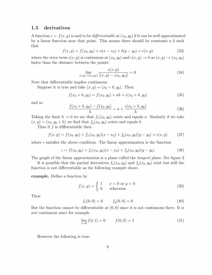
The graph of the linear approximation is a plane called the tangent plane. See figure 2It is possible that the partial derivatives fx(x0, y0) and fy(x0, y0) exist but still the
function is not differentiable as the following example shows
example. Define a function by
f(x, y) =
{1 x = 0 or y = 00 otherwise
(39)
Thenfx(0, 0) = 0 fy(0, 0) = 0 (40)
But the function cannot be differentiable at (0, 0) since it is not continuous there. It isnot continuous since for example
limt→0
f(t, t) = 0 f(0, 0) = 1 (41)
However the following is true:
8
Figure 2: tangent plane
Theorem 2 If the partial derivatives fx, fy exist and are continuous near (x0, y0) (i.ein a little disc centered on (x0, y0)) then f is differentiable at (x0, y0).
problem: Show the function f(x, y) = y3 + 3x2y2 is differentiable at any point andfind the linear approximation (tangent plane) at (1, 1).
solution: This has partial derivatives
fx(x, y) = 6xy2 fy(x, y) = 3y2 + 6x2y (42)
at any point and they are continuous. Thus the function is differentiable. The tangentplane at (1, 1) is
z =f(1, 1) + fx(1, 1)(x− 1) + fy(1, 1)(y − 1)
=4 + 6(x− 1) + 9(y − 1)
=6x+ 9y − 11
(43)
Next consider a function from Rn to R written y = f(x) = f(x1, . . . , xn). We say fis differentiable at x0 = (x0
1, . . . x0n) if there is a vector a = (a1, . . . , an) such that
f(x) = f(x0) + a · (x− x0) + ε(x) (44)
9

where as before
limx→x0
ε(x)
|x− x0|= 0 (45)
If it is true then we find as before that the vector must be
a = (fx1(x0), . . . , fxn(x0)) ≡ (∇f)(x0) (46)
also called the gradient of f at x0. Thus we have
f(x) = f(x0) + (∇f)(x0) · (x− x0) + ε(x) (47)
Finally consider a function y = f(x) from Rn to Rm. We write the points and thefunction as column vectors:
y =
y1...ym
=
f1(x)...
fm(x)
x =
x1...xn
(48)
The function is differentiable at x0 is there is an m× n matrix (m rows, n columns) Asuch that
f(x) = f(x0) + A(x− x0) + ε(x) (49)
where the error ε(x) ∈ Rm satisfies
limx→x0
|ε(x)||x− x0|
= 0 (50)
By considering each component separately we find that the ith row of A must be thethe gradient of fi at x0. Thus
A = Df(x0) ≡
f1,x1(x0) · · · f1,xn(x0)
......
fm,x1(x0) · · · fm,xn(x0)
(51)
This matrix Df(x0) made up of all the partial derivatives of f at x0 is the derivativeof f at x0. Thus we have
f(x) = f(x0) +Df(x0)(x− x0) + ε(x) (52)
The derivative is also written
Df ≡
∂y1/∂x1 · · · ∂y1/∂xn...
...∂ym/∂x1 · · · ∂ym/∂xn
(53)
10

problem: Consider the function from R2 to R2 given by(y1
y2
)=
(f1(x)f2(x)
)=
((x1 + x2 + 1)2
x1(x2 + 3)
)(54)
Find the linear approximation at (0, 0)
solution: The derivative is
Df =
(∂y1/∂x1 ∂y1/∂x2
∂y2/∂x1 ∂y2/∂x2
)=
(2(x1 + x2 + 1) 2(x1 + x2 + 1)
x2 + 3 x1
)(55)
The linear approximation is
y = f(0) +Df(0)(x− 0) (56)
or (y1
y2
)=
(10
)+
(2 23 0
)(x1
x2
)=
(2x1 + 2x2 + 1
3x1
)(57)
1.6 the chain rule
If f : Rn → Rm (i.e. f is a function from Rn to Rm) and p : Rk → Rn, then there is acomposite function h : Rk → Rm defined by
h(x) = f(p(x)) (58)
and we also write h = f ◦ p. We can represent the situation by the diagram:
Rk -p
Rn
?
f
Rm
@@@@Rh
The chain gives a formula for the derivatives of the composite function h in termsof the derivatives of f and p. We start with some special cases.
k=1,n=2,m=1 In this case the functions have the form
u =f(x, y)
x =p1(t) y = p2(t)(59)
and the composite isu = h(t) = f(p1(t), p2(t)) (60)
11

Theorem 3 (chain rule) If f and p are differentiable, then so is the composite h = f ◦pand the derivative is
h′(t) = fx(p1(t), p2(t))p′1(t) + fy(p1(t), p2(t))p′1(t) (61)
The idea of the proof is as follows. Since f is differentiable
h(t+ ∆t)− h(t) =f((p1(t+ ∆t), p2(t+ ∆t))− f(p1(t), p2(t))
=fx(p1(t), p2(t))(p1(t+ ∆t)− p2(t)
)+ fy(p1(t), p2(t))
(p2(t+ ∆t)− p2(t)
)+ε(p1(t+ ∆t), p2(t+ ∆t))
(62)
Now divide by ∆t and let ∆t → 0. One has to show that the error term goes to zeroand the result follows.
This form of the chain rule can also be written in the concise form
du
dt=∂u
∂x
dx
dt+∂u
∂y
dy
dt(63)
But one must keep in mind that ∂u/∂x and ∂u/∂y are to be evaluated at x = p1(t), y =p2(t). Also note that on the left u stands for the function u = h(t) while on the rightit stands for the function u = f(x, y).
example: Suppose u = x2 + y2 and x = cos t , y = sin t. Find du/dt. We have
du
dt=∂u
∂x
dx
dt+∂u
∂y
dy
dt
=2x(− sin t) + 2y cos t
=2 cos t(− sin t) + 2 sin t cos t
=0
(64)
(This is to be expected since the composite is u = 1).
example: Suppose u =√
2 + x2 + y2 and x = et , y = e2t. Find du/dt at t = 0. Att = 0 we have x = 1, y = 1 and so
du
dt=∂u
∂x
dx
dt+∂u
∂y
dy
dt
=x√
2 + x2 + y2et +
y√2 + x2 + y2
2e2t
=1
2· 1 +
1
2· 2 =
3
2
(65)
12
k=1,n,m=1 In this case the functions have the form
u = f(x1, . . . xn)
x1 = p1(t), . . . , xn = pn(t)(66)
and the composite isu = h(t) = f(p1(t), · · · , pn(t)) (67)
The chain rule says
h′(t) = fx1(p1(t), · · · , pn(t))p′1(t) + · · ·+ fxn(p1(t), · · · , pn(t))p′n(t) (68)
It can also be writtendu
dt=
∂u
∂x1
dx1
dt+ · · ·+ ∂u
∂xn
dxndt
(69)
k=2,n=2,m=2 In this case the functions have the form
u = f1(x, y) v = f2(x, y)
x = p1(s, t) y = p2(s, t)(70)
and the composite is
u = h1(s, t) = f1(p1(s, t), p2(s, t)) v = h2(s, t) = f2(p1(s, t), p2(s, t)) (71)
Taking partial derivatives with respect to s, t we can use the formula from the casek=1,n=2,m=1 to obtain
∂u
∂s=∂u
∂x
∂x
∂s+∂u
∂y
∂y
∂s∂u
∂t=∂u
∂x
∂x
∂t+∂u
∂y
∂y
∂t∂v
∂s=∂v
∂x
∂x
∂s+∂v
∂y
∂y
∂s∂v
∂t=∂v
∂x
∂x
∂t+∂v
∂y
∂y
∂t
(72)
Here derivatives with respect to x, y are to be evaluated at x = p1(s, t), y = p2(s, t).This can also be written as a matrix product:(
∂u/∂s ∂u/∂t∂v/∂s ∂v/∂t
)=
(∂u/∂x ∂u/∂y∂v/∂x ∂v/∂y
)(∂x/∂s ∂x/∂t∂y/∂s ∂y/∂t
)(73)
13
These matrices are just the derivatives of the various functions and the last equationcan be written
(Dh)(s, t) = (Df)(p(s, t))(Dp)(s, t) (74)
The last form holds in the general case. If p : Rk → Rn and f : Rn → Rm aredifferentiable then the composite function h = f ◦ p : Rk → Rm is differentiable and
(Dh)(x)︸ ︷︷ ︸m×k matrix
= (Df)(p(x))︸ ︷︷ ︸m×n matrix
(Dp)(x)︸ ︷︷ ︸n×k matrix
(75)
In other words the derivative of a composite is the matrix product of the derivatives ofthe two elements. All forms of the chain rule are special cases of this equation.
1.7 implicit function theorem -I
Suppose we have an equation of the form
f(x, y, z) = 0 (76)
Can we solve it for z?. More precisely, is it the case that for each x, y in some domainthere is a unique z so that f(x, y, z) = 0? If so one can define an implicit functionby z = φ(x, y). Geometrically points satisfying f(x, y, z) = 0 are a surface and we areasking whether the surface is the graph of a function.
Suppose there is an implicit function. Then
f(x, y, φ(x, y)) = 0 (77)
Assuming everything is differentiable we can take partial derivatives of this equation.By the chain rule we have
0 =∂
∂x[f(x, y, φ(x, y))] =fx(x, y, φ(x, y)) + fz(x, y, φ(x, y))φx(x, y)
0 =∂
∂y[f(x, y, φ(x, y))] =fy(x, y, φ(x, y)) + fz(x, y, φ(x, y))φy(x, y)
(78)
Solve this for φx(x, y) and φy(x, y) and get
φx(x, y) =− fx(x, y, φ(x, y))
fz(x, y, φ(x, y))
φy(x, y) =− fy(x, y, φ(x, y))
fz(x, y, φ(x, y))
(79)
14

This can also be written in the form
∂z
∂x=− ∂f/∂x
∂f/∂z
∂z
∂y=− ∂f/∂y
∂f/∂z
(80)
keeping in mind that the right side is evaluated at z = φ(x, y).For this to work we need that ∂f/∂z 6= 0. If this holds and if we restrict attention
to a small region then there always is an implicit function. This is the content of thefollowing
Theorem 4 (implicit function theorem) Let f(x, y, z) have continuous partial deriva-tives near some point (x0, y0, z0). If
f(x0, y0, z0) =0
fz(x0, y0, z0) 6=0(81)
Then for every (x, y) near (x0, y0) there is a unique z near z0 such that f(x, y, z) = 0.The implicit function z = φ(x, y) satisfies z0 = φ(x0, y0) and has continuous partialderivatives near (x0, y0) which satisfy the equations (79).
The theorem does not tell you what φ is or how to find it, only that it exists.However if we take the equations (79) at the special point (x0, y0) we find
φx(x0, y0) =− fx(x0, y0, z0)
fz(x0, y0, z0)
φx(x0, y0) =− fx(x0, y0, z0)
fz(x0, y0, z0)
(82)
and these quantities can be computed.
example: Suppose the equation is
f(x, y, z) = x2 + y2 + z2 − 1 = 0 (83)
which describes the surface of a sphere. Is there an implicit function z = φ(x, y) neara particular point (x0, y0, z0) on the sphere?
We have the derivatives
fx(x, y, z) = 2x fy(x, y, z) = 2y fz(x, y, z) = 2z (84)
15
Then fz(x0, y0, z0) = 2z0 is not zero if z0 6= 0. So by the theorem there is an implicitfunction z = φ(x, y) near a point with z0 6= 0 and
∂z
∂x=− fx
fz= −x
z∂z
∂y=− fy
fz= −y
z
(85)
This example is special in that we can find the implicit function exactly and socheck these results. The implicit function is
z = ±√
1− x2 − y2 (86)
with the plus sign if z0 > 0 and the minus sign if z0 < 0. In either case we have theexpected result
∂z
∂x=± 1
2(1− x2 − y2)−1/2(−2x) = −x
z∂z
∂y=± 1
2(1− x2 − y2)−1/2(−2y) = −y
z
(87)
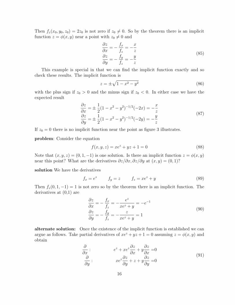
If z0 = 0 there is no implicit function near the point as figure 3 illustrates.
problem: Consider the equation
f(x, y, z) = xez + yz + 1 = 0 (88)
Note that (x, y, z) = (0, 1,−1) is one solution. Is there an implicit function z = φ(x, y)near this point? What are the derivatives ∂z/∂x, ∂z/∂y at (x, y) = (0, 1)?
solution We have the derivatives
fx = ez fy = z fz = xez + y (89)
Then fz(0, 1,−1) = 1 is not zero so by the theorem there is an implicit function. Thederivatives at (0,1) are
∂z
∂x=− fx
fz= − ez
xez + y= −e−1
∂z
∂y=− fy
fz= − z
xez + y= 1
(90)
alternate solution: Once the existence of the implicit function is established we canargue as follows. Take partial derivatives of xez + yz+ 1 = 0 assuming z = φ(x, y) andobtain
∂
∂x: ez + xez
∂z
∂x+ y
∂z
∂x=0
∂
∂y: xez
∂z
∂y+ z + y
∂z
∂y=0
(91)
16
Figure 3: There is an implicit function near points with z0 6= 0, but not near pointswith z0 = 0.
Now put in the point (x, y, z) = (0, 1,−1) and get
e−1 +∂z
∂x=0
−1 +∂z
∂y=0
(92)
Solving for the derivatives gives the same result.
Some remarks:
1. Why is the implicit function theorem true? Instead of solving f(x, y, z) = 0 forz near (x0, y0, z0) one could make a linear approximation and try to solve that.Taking into account that f(x0, y0, z0) = 0 the linear approximation is
fx(x0, y0, z0)(x− x0) + fy(x0, y0, z0)(y − y0) + fz(x0, y0, z0)(z − z0) = 0 (93)
If fz(x0, y0, z0) 6= 0 this can be solved by
z = z0 −fx(x0, y0, z0)
fz(x0, y0, z0)(x− x0)− fy(x0, y0, z0)
fz(x0, y0, z0)(y − y0) (94)
17

and this has the expected derivatives. To prove the theorem one has to arguethat since the actual function is near the linear approximation there is an implicitfunction in that case as well.
2. Here are some variations of the implicit function theorem
(a) If f(x, y) = 0 one can solve for y = φ(x) near any point where fy 6= 0 anddy/dx = −fx/fy.
(b) If f(x, y, z) = 0 one can solve for x = φ(y, z) near any point where fx 6= 0and ∂x/∂y = −fy/fx and ∂x/∂z = −fz/fx
(c) If f(x, y, z, w) = 0 one can solve for w = φ(x, y, z) near any point wherefw 6= 0 and ∂w/∂x = −fx/fw, etc.
3. One can also find higher derivatives of the implicit function. If f(x, y, z) = 0defines z = φ(x, y) and
φx(x, y) = −fx(x, y, φ(x, y))
fz(x, y, φ(x, y))(95)
then one can find φxx, φxy by further differentiation.
example: f(x, y, z) = x2 + y2 + z2 − 1 = 0 defines z = φ(x, y) which satisfies
∂z
∂x= −x
z(96)
Keeping in mind that z is a function of x, y further differentiation yields
∂2z
∂x2= −
(z − x ∂z/∂x
z2
)= −
(z − x(−x/z)
z2
)=−z2 − x2
z3(97)
Since x2 + y2 + z2 = 1 this can also be written as (y2 − 1)/z3. Similarly
∂2z
∂x∂y=−xyz3
(98)
1.8 implicit function theorem -II
We give another version of the implicit function theorem. Suppose we have a pair ofequations of the form
F (x, y, u, v) =0
G(x, y, u, v) =0(99)
18
Can we solve them for u, v as functions of x, y? More precisely is it the case that foreach x, y in some domain there is a unique u, v so that the equations are satisfied. If itis so we can define implicit functions
u =f(x, y)
v =g(x, y)(100)
If the implicit functions exist we have
F (x, y, f(x, y), g(x, y)) =0
G(x, y, f(x, y), g(x, y)) =0(101)
Take partial derivatives with respect to x and y and get
Fx + Fufx + Fvgx =0
Gx +Gufx +Gvgx =0
Fy + Fufy + Fvgy =0
Gy +Gufy +Gvgy =0
(102)
These equations can be written as the matrix equations(Fu FvGu Gv
)(fxgx
)=
(−Fx−Gx
)(Fu FvGu Gv
)(fygy
)=
(−Fy−Gy
) (103)
Note that the matrix on the left is the derivative of the function
(u, v)→ (F (x, y, u, v), G(x, y, u, v)) (104)
for fixed (x, y). If the determinant of this matrix is not zero we can solve for the partialderivatives fx, gx, fy, gy. One finds for example
fx =
det
(−Fx Fv−Gx Gv
)det
(Fu FvGu Gv
) (105)
The determinant of the matrix is called the Jacobian determinant and is given aspecial symbol
∂(F,G)
∂(u, v)≡ det
(Fu FvGu Gv
)≡ FuGv − FvGu (106)
19

With this notation the equations for the four partial derivatives can be written
∂u
∂x=− ∂(F,G)
∂(x, v)/∂(F,G)
∂(u, v)
∂v
∂x=− ∂(F,G)
∂(u, x)/∂(F,G)
∂(u, v)
∂u
∂y=− ∂(F,G)
∂(y, v)/∂(F,G)
∂(u, v)
∂v
∂y=− ∂(F,G)
∂(u, y)/∂(F,G)
∂(u, v)
(107)
where u = f(x, y), v = g(x, y) on the right. This holds provided ∂(F,G)/∂(u, v) 6= 0and this is the key condition in the following theorem which guarantees the existenceof the implicit functions.
Theorem 5 (implicit function theorem) Let F,G have continuous partial derivativesnear some point (x0, y0, u0, v0). If
F (x0, y0, u0, v0) =0
G(x0, y0, u0, v0) =0(108)
and [∂(F,G)
∂(u, v)
](x0, y0, u0, v0) 6= 0 (109)
Then for every (x, y) near (x0, y0) there is a unique (u, v) near (u0, v0) such thatF (x, y, u, v) = 0 and G(x, y, u, v) = 0. The implicit functions u = f(x, y), v = g(x, y)satisfy u0 = f(x0, y0), v0 = g(x0, y0) and have continuous partial derivative which satisfythe equations (107).
problem: Consider the equations
F (x, y, u, v) = x2 − y2 + 2uv − 2 =0
G(x, y, u, v) = 3x+ 2xy + u2 − v2 =0(110)
Note that (x, y, u, v) = (0, 0, 1, 1) is a solution. Are there implicit functions u =f(x, y), v = g(x, y) near (0, 0)? What are the derivatives ∂u/∂x, ∂v/∂x at (x, y) =(0, 0)?
solution: First compute
∂(F,G)
∂(u, v)= det
(Fu FvGu Gv
)= det
(2v 2u2u −2v
)= −4(u2 + v2) = −8 (111)
20

Since this is not zero the implicit functions exist by the theorem. We also compute
∂(F,G)
∂(x, v)= det
(Fx FvGx Gv
)= det
(2x 2u
3 + 2y −2v
)= −4xv − 2u(3 + 2y) = −6
(112)
and
∂(F,G)
∂(u, x)= det
(Fu FxGu Gx
)= det
(2v 2x2u 3 + 2y
)= 2v(3 + 2y)− 4ux = 6 (113)
Then∂u
∂x= −−6
−8= −3
4
∂v
∂x= − 6
−8=
3
4(114)
alternate solution: Assuming the implicit functions exist differentiate the equationsF = 0, G = 0 with respect to x assuming u = f(x, y), v = g(x, y). This gives
2x+ 2v∂u
∂x+ 2u
∂v
∂x=0
3 + 2y + 2u∂u
∂x− 2v
∂v
∂x=0
(115)
Now put in the point (0, 0, 1, 1) and get
2∂u
∂x+ 2
∂v
∂x=0
3 + 2∂u
∂x− 2
∂v
∂x=0
(116)
This again has the solution ∂u/∂x = −3/4, ∂v/∂x = 3/4.
1.9 inverse functions
Suppose we have a function f from U ⊂ R2 to V ⊂ R2 which we write in the form
x =f1(u, v)
y =f2(u, v)(117)
Suppose further for every (x, y) in V there is a unique (u, v) in U such that x =f1(u, v), y = f2(u, v). (0ne says the function is one-to-one and onto.) Then there is aan inverse function g from V to U defined by
u =g1(x, y)
v =g2(x.y)(118)
21

Figure 4: inverse function
So g sends every point back where it came from. See figure 4. We have
(g ◦ f)(u, v) =(u, v)
(f ◦ g)(x, y) =(x, y)(119)
We write g = f−1.
example: Suppose the function is
x =au+ bv
y =cu+ dv(120)
defined on all of R2. This can also be written in matrix form(xy
)=
(a bc d
)(uv
)(121)
This is invertible if we can solve the equation for (u, v) which is possible if and only if
det
(a bc d
)= ad− bc 6= 0 (122)
22
The inverse function is given by the inverse matrix(uv
)=
(a bc d
)−1(xy
)(123)
where (a bc d
)−1
=1
ad− bc
(d −b−c a
)(124)
example: Consider the function
x =r cos θ
y =r sin θ(125)
fromU = {(r, θ) : r > 0, 0 ≤ θ < 2π} (126)
toV = {(x, y) : (x, y) 6= 0} (127)
This function sends (r, θ) to the point with polar coordinates (r, θ). See figure 5. Thefunction is invertible since every point (x, y) in V has unique polar coordinates (r, θ)in U . (It would not be invertible if we took U = R2 since (r, θ) and (r, θ+ 2π) are sentto the same point ). For (x, y) in the first quadrant the inverse is
r =√x2 + y2
θ = tan−1(yx
) (128)
1.10 inverse function theorem
Continuing the discussion of the previous section suppose that f has an inverse functiong and that both are differentiable. Then differentiating (f ◦ g)(x, y) = (x, y) we find bythe chain rule
(Df)(g(x, y)) (Dg)(x, y) = I I =
(1 00 1
)(129)
and so the derivative of the inverse function is the matrix inverse
(Dg)(x, y) = [(Df)(g(x, y))]−1 (130)
It is not always easy to tell whether an inverse function exists. The followingtheorem can be helpful.
23
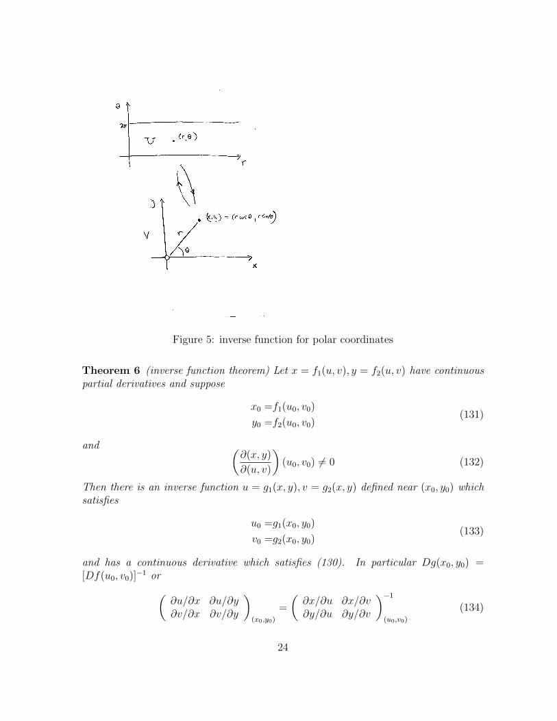
Figure 5: inverse function for polar coordinates
Theorem 6 (inverse function theorem) Let x = f1(u, v), y = f2(u, v) have continuouspartial derivatives and suppose
x0 =f1(u0, v0)
y0 =f2(u0, v0)(131)
and (∂(x, y)
∂(u, v)
)(u0, v0) 6= 0 (132)
Then there is an inverse function u = g1(x, y), v = g2(x, y) defined near (x0, y0) whichsatisfies
u0 =g1(x0, y0)
v0 =g2(x0, y0)(133)
and has a continuous derivative which satisfies (130). In particular Dg(x0, y0) =[Df(u0, v0)]−1 or(
∂u/∂x ∂u/∂y∂v/∂x ∂v/∂y
)(x0,y0)
=
(∂x/∂u ∂x/∂v∂y/∂u ∂y/∂v
)−1
(u0,v0)
(134)
24
Proof. The inverse exists if for each (x, y) near (x0, y0) there is a unique (u, v) near(u0, v0) such that
F (x, y, u, v) ≡ f1(u, v)− x =0
G(x, y, u, v) ≡ f2(u, v)− y =0(135)
This follows by the implicit functions theorem since (x0, y0, u0, v0) is one solution andat this point
∂(F,G)
∂(u, v)= det
(Fu FvGu Gv
)= det
(f1,u f1,v
f2,u f2,v
)=∂(x, y)
∂(u, v)6= 0
The differentiability of the inverse also follows from the implicit function theorem.
problem: Consider the function
x =u+ v2
y =u2 + v(137)
which sends (u, v) = (1, 2) to (x, y) = (5, 3). Show that the function is invertible near(1, 2) and find the partial derivatives of the inverse function at (5, 3).
solution: We have(∂x/∂u ∂x/∂v∂y/∂u ∂y/∂v
)=
(1 2v
2u 1
)=
(1 42 1
)at (1, 2) (138)
Therefore∂(x, y)
∂(u, v)= det
(1 42 1
)= −7 at (1, 2) (139)
This is not zero so the inverse exists by the theorem and sends (5, 3) to (1, 2). We havefor the derivatives(
∂u/∂x ∂u/∂y∂v/∂x ∂v/∂y
)(5,3)
=
(∂x/∂u ∂x/∂v∂y/∂u ∂y/∂v
)−1
(1,2)
=
(1 42 1
)−1
=
(−1/7 4/72/7 −1/7
) (140)
alternate solution: Differentiate x = u + v2, y = u2 + v assuming u, v are functionsof x, y, then put in the point.
25

1.11 maxima and minima
Let f(x) = f(x1, . . . , xn) be a function from Rn to R and let x0 = (x01, . . . x
0n) be a point
in Rn. We say that f has a local maximum at x0 if f(x) ≤ f(x0) for all x near x0. Wesay that f has a local minimum at x0 if f(x) ≥ f(x0) for all x near x0.
Theorem 7 If f is differentiable at x0 and f has a local maximum or minimum at x0
then all partial derivatives vanish at the point, i.e.
fx1(x0) = · · · = fxn(x0) = 0 (141)
Proof. For any h = (h1, . . . , hn) ∈ Rn consider the function F (t) = f(x0 + th) ofthe single variable t. If f has a local maximum or minimum at x0 then F has a localmaximum or minimum at t = 0. By the chain rule F (t) is differentiable and and it isa result of elementary calculus that F ′(0) = 0. But the chain rule says
F ′(t) =n∑i=1
fxi(x0 + th)
d(x0i + thi)
dt=
n∑i=1
fxi(x0 + th)hi (142)
Thus
0 = F ′(0) =n∑i=1
fxi(x0)hi (143)
Since this is true for any h it must be that fxi(x0) = 0.
A point x0 with fxi(x0) = 0 is called a critical point for f . We have seen that if f
is has a local maximum or minimum at x0 then it is a critical point. We are interestedwhether the converse is true. If x0 is a critical point is it a local maximum or minimumfor f? Which is it?
To answer this question consider again F (t) = f(x0 + th) and suppose f is manytimes differentiable. By Taylor’s theorem for one variable we have
F (1) = F (0) + F ′(0) +1
2F ′′(0) +
1
6F ′′′(s) (144)
for some s between 0 and 1. But F ′(t) is computed above, and similarly we have
F ′′(t) =n∑i=1
n∑j=1
fxixj(x0 + th)hihj
F ′′′(t) =n∑i=1
n∑j=1
n∑k=1
fxixjxk(x0 + th)hihjhk
(145)
26
Then the Taylor’s expansion becomes
f(x0 + h) = f(x0) +n∑i=1
fxi(x0)hi +
1
2
n∑i=1
n∑j=1
fxixj(x0)hihj +R(h) (146)
This is an example of a multivariable Taylor’s theorem with remainder. The remainderR(h) = F ′′′(s)/6 is small if h is small and one can show that there is a constant C suchthat for h small |R(h)| ≤ C|h|3.
Now suppose x0 is a critical point so the first derivatives vanish. Also define amatrix of second derivatives
A =
fx1,x1(x0) · · · fx1,xn(x0)
......
fxn,x1(x0) · · · fxn,xn(x0)
(147)
called the Hessian of f at x0. Then we can write our expansion as
f(x0 + h) = f(x0) +1
2h · Ah+R(h) (148)
We are interested in whether f(x0 + h) is greater than or less than f(x0) for |h| small.Then idea is that since R(h) is much smaller than 1
2h · Ah it is the latter term which
determines the answer.A n×n matrix A is called positive definite if there is a constant M so h·Ah > M |h|2
for all h 6= 0. It is called negative definite if h · Ah < −M |h|2 for all h 6= 0.
Theorem 8 Let x0 be a critical point for f and suppose the Hessian A has detA 6= 0.
1. If A is positive definite then f has a local minimum at x0.
2. If A is negative definite then f has a local maximum at x0.
3. Otherwise f has a saddle point at x0, i.e f increases in some directions anddecreases in other directions as you move away from x0.
Proof. We prove the first statement. We have h · Ah > M |h|2. If also |h| ≤ M/4C.then
|R(h)| ≤ C|h|3 ≤ 1
4M |h|2 (149)
Therefore
f(x0 + h) ≥ f(x0) +1
2M |h|2 − 1
4M |h|2 (150)
or
f(x0 + h) ≥ f(x0) +1
4M |h|2 (151)
27
Thus f(x0 + h) > f(x0) for 0 < |h| ≤ M/4C which means we have a strict localmaximum at x0.
Thus our problem is to decide whether or not A is positive or negative definite.For any symmetric matrix A one can show that A is positive definite if and only ifall eigenvalues are postive and A is negative definite if and only if all eigenvalues arenegative. Recall that λ is an eigenvalue if there is a vector v 6= 0 such that Av = λv.One can find the eigenvalues by solving the equation
det(A− λI) = 0 (152)
where I is the identity matrix.
example: Consider the function
f(x, y) = exp
(−x
2
2− y2
2+ x+ y
)(153)
The critical points are solutions of
fx =(−x+ 1) exp
(−x
2
2− y2
2+ x+ y
)= 0
fy =(−y + 1) exp
(−x
2
2− y2
2+ x+ y
)= 0
(154)
Thus the only critical point is (x, y) = (1, 1). The second derivatives at this point are
fxx =(x2 − 2x) exp
(−x
2
2− y2
2+ x+ y
)= −e
fxy =(−x+ 1)(−y + 1) exp
(−x
2
2− y2
2+ x+ y
)= 0
fyy =(y2 − 2y) exp
(−x
2
2− y2
2+ x+ y
)= −e
(155)
Thus the Hessian is
A =
(fxx fxyfyx fyy
)=
(−e 00 −e
)(156)
It has eigenvalues −e,−e which are negative. Hence A is negative definite and thefunction has a local maximum at (1, 1).
example: Consider the function
f(x, y) = x sin y (157)
28

The critical points are solutions of
fx = sin y = 0
fy =x cos y = 0(158)
These are points with x = 0 and y = 0,±π,±2π, · · · . The Hessian is
A =
(fxx fxyfyx fyy
)=
(0 cos y
cos y −x sin y
)(159)
At points (0,±π), (0,±3π), . . . this is
A =
(0 −1−1 0
)(160)
At points (0, 0), (0,±2π), . . . this is
A =
(0 11 0
)(161)
In either case the eigenvalues are solutions of
det(A− λI) = det
(−λ ±1±1 −λ
)= λ2 − 1 = 0 (162)
Thus the eigenvalues are λ = ±1. Since they have both signs every critical point is asaddle point.
1.12 differentiation under the integral sign
Theorem 9 If f(t, x), (∂f/∂t)(t, x) exist and are continuous
d
dt
[∫ b
a
f(t, x)dx
]=
∫ b
a
∂f
∂t(t, x) dx (163)
Proof. Form the difference quotient∫ baf(t, x+ h)−
∫ baf(t, x)
h=
∫ b
a
f(t, x+ h)− f(t, x)
h(164)
and take the limit h → 0. The only issue is whether we can take the limit under theintegral sign on the right. This can be justified under the hypotheses of the theorem.
29

example:
d
dt
[∫ 1
0
log(x2 + t2)dx
]=
∫ 1
0
2t
x2 + t2dx
=[2 tan−1
(xt
)]x=1
x=0
=2 tan−1
(1
t
) (165)
problem: Find ∫ 1
0
√x− 1
log xdx (166)
solution: We solve a more general problem which is to evaluate
φ(t) =
∫ 1
0
xt − 1
log xdx (167)
Then φ(1/2) is the answer to the original problem. Differentiating under the integralsign and taking account that d(xt)/dt = xt log x we have
φ′(t) =
∫ 1
0
xt dx =
[xt+1
t+ 1
]x=1
x=0
=1
t+ 1(168)
Henceφ(t) = log(t+ 1) + C (169)
for some constant C. But we know φ(0) = 0 so we must have C = 0. Thus φ(t) =log(t+ 1) and the answer is φ(1/2) = log(3/2).
1.13 Leibniz’ rule
The following is a generalization of the previous result where we allow the endpointsto be functions of t.
Theorem 10
d
dt
[∫ b(t)
a(t)
f(t, x)dx
]= f
(t, b(t)
)b′(t)− f
(t, a(t)
)a′(t) +
∫ b(t)
a(t)
∂f
∂t(t, x) dx (170)
30
Proof. Let
F (b, a, t) =
∫ b
a
f(t, x) dx (171)
What we want is the derivative of F (b(t), a(t), t) and by the chain rule this is
d
dt[F (b(t), a(t), t)]
= Fb(b(t), a(t), t)b′(t) + Fa(b(t), a(t), t)a′(t) + Ft(b(t), a(t), t)(172)
But
Fb(b, a, t) = f(t, b) Fa(b, a, t) = −f(t, a) Ft(b, a, t) =
∫ b
a
∂f
∂t(t, x) dx (173)
which gives the result.
example:
d
dt
[∫ t2
t
sin(t2 + x2)dx
]
= sin(t2 + x2)|x=t2d(t2)
dt− sin(t2 + x2)|x=t
d(t)
dt+
∫ t2
t
∂
∂tsin(t2 + x2)dx
= sin(t2 + t4)2t− sin(2t2) + 2t
∫ t2
t
cos(t2 + x2)dx
(174)
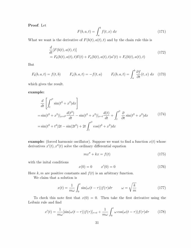
example: (forced harmonic oscillator). Suppose we want to find a function x(t) whosederivatives x′(t), x′′(t) solve the ordinary differential equation
mx′′ + kx = f(t) (175)
with the inital conditionsx(0) = 0 x′(0) = 0 (176)
Here k,m are positive constants and f(t) is an arbitrary function.We claim that a solution is
x(t) =1
mω
∫ t
0
sin(ω(t− τ))f(τ)dτ ω =
√k
m(177)
To check this note first that x(0) = 0. Then take the first derivative using theLeibniz rule and find
x′(t) =1
mω[sin(ω(t− τ))f(τ)]τ=t +
1
mω
∫ t
0
ω cos(ω(t− τ))f(τ)dτ (178)
31

The first term is zero and we also note that x′(0) = 0. Taking one more derivativeyields
x′′(t) =1
m[cos(ω(t− τ))f(τ)]τ=t +
1
mω
∫ t
0
(−ω2) sin(ω(t− τ))f(τ)dτ (179)
which is the same as
x′′(t) =1
mf(t)− ω2x(t) (180)
Now multiply by m, use mω2 = k and we recover the differential equation.
1.14 calculus of variations
We consider the problem of finding maximima and minima for a functional - i.e. for afunction of functions.
As an example consider the problem of finding the curve between two points (x0, y0)and (x1, y1) which has the shortest length. We assume that there is such a curve andthat it it is the graph of a function y = y(x) with y(x0) = y0 and y(x1) = y1. Thelength of such a curve is
I(y) =
∫ x1
x0
√1 + y′(x)2dx (181)
and we seek to find the function y = y(x) which gives the minimum value.More generally suppose we have a function F (x, y, y′) of three real variables (x, y, y′).
For any differentiable function y = y(x) satisfying y(x0) = y0 and y(x1) = y1 form theintegral
I(y) =
∫ x1
x0
F (x, y(x), y′(x))dx (182)
The question is which function y = y(x) minimizes (or maximizes) the functional I(y).We are looking for a local minimum (or maximum), that is we want to find a functiony such that I(y) ≥ I(y) for all functions y near to y in the sense that y(x) is close toy(x) for all x0 ≤ x ≤ x1.
Theorem 11 If y = y(x) is a local maximum or minimum for I(y) with fixed endpointsthen it satisfies
Fy(x, y(x), y′(x))− d
dx(Fy′(x, y(x), y′(x)) = 0 (183)
Remarks.
1. The equation is called Euler’s equation and is abreviated as
Fy −d
dxFy′ = 0 (184)
32

2. Note that y, y′ mean two different things in Euler’s equation. First one evaluatesthe partial derivatives Fy, Fy′ treating y, y′ as independent variables. Then incomputing d/dx one treats y, y′ as a function and its derivative.
3. The converse may not be true, i.e solutions of Euler’s equation are not necessarilymaxima or minima. They are just candidates and one should decide by othercriteria.
proof: Suppose y = y(x) is a local minimum. Pick any differentiable function η(x)defined for x0 ≤ x ≤ x1 and satisfying η(x0) = η(x1) = 0. Then for any real number tthe function
yt(x) = y(x) + tη(x) (185)
is differentiable with respect to x and satisfies yt(x0) = yt(x1) = 0. Consider thefunction
J(t) = I(yt) =
∫ x1
x0
F (x, yt(x), y′t(x))dx (186)
Since yt is near y0 = y for t small, and since y0 is a local minimum for I, we have
J(t) = I(yt) ≥ I(y0) = J(0) (187)
Thus t = 0 is a local minimum for J(t) and it follows that J ′(0) = 0.To see what this says we differentiate under the integral sign and compute
J ′(t) =
∫ x1
x0
∂
∂tF (x, yt(x), y′t(x))dx
=
∫ x1
x0
(Fy(x, yt(x), y′t(x))
∂
∂t(yt(x)) + Fy′(x, yt(x), y′t(x))
∂
∂t(y′t(x))
)dx
=
∫ x1
x0
(Fy(x, yt(x), y′t(x))η(x) + Fy′(x, yt(x), y′t(x))η′(x)) dx
(188)
Here in the second step we have used the chain rule. Now in the second term integrateby parts taking the derivative off η′(x) = (d/dx)η and putting it on Fy′(x, yt(x), y′t(x))The term involving the endpoints vanishes because η(x0) = η(x1) = 0. Then we have
J ′(t) =
∫ x1
x0
(Fy(x, yt(x), y′t(x))− d
dxFy′(x, yt(x), y′t(x))
)η(x)dx (189)
Now put t = 0 and get
0 = J ′(0) =
∫ x1
x0
(Fy(x, y(x), y′(x))− d
dxFy′(x, y(x), y′(x))
)η(x)dx (190)
33

Since this is true for an arbitrary function η it follows that the expression in parenthesesmust be zero which is our result. 1
example: We return to the problem of finding the curve between two points with theshortest length. That is we seek to minimize
I(y) =
∫ x1
x0
√1 + y′(x)2dx (191)
This has the form (182) with
F (x, y, y′) =√
1 + (y′)2 (192)
The minimizer must satisfy Euler’s equation. Since Fy = 0 and Fy′ = y′/√
1 + (y′)2
this says
Fy −d
dxFy′ =
d
dx
[y′√
1 + (y′)2
]= 0 (193)
Evaluating the derivatives yields√1 + (y′)2y′′ − (y′)2y′′/
√1 + (y′)2
1 + (y′)2= 0 (194)
Now multiple by (1 + (y′)2)3/2 and get
(1 + (y′)2)y′′ − (y′)2y′′ = 0 (195)
which is the same as y′′ = 0. Thus the minimizer must have the form y = ax + b forsome constants a, b. So the shortest distance between two points is along a straight lineas expected.
example: The problem is to find the function y = y(x) with y(0) = 0 and y(1) = 1which minimizes the integral
I(y) =1
2
∫ 1
0
(y(x)2 + (y′(x))2)dx (196)
and again we assume there is such a minimizer. The integral has the form (182) with
F (x, y, y′) =1
2(y2 + (y′)2) (197)
1In general if f is a continuous function∫ b
af(x)dx = 0 does not imply that f ≡ 0. However it is
true if f(x) ≥ 0. If∫ b
af(x)η(x)dx = 0 for any continuous function η then we can take η(x) = f(x)
and get∫ b
af(x)2dx = 0, hence f(x)2 = 0, hence f(x) = 0. This is not quite the situation above since
we also restriced η to vanish at the endpoints. But the conclusion is stil valid.
34
Then Euler’s equation says
Fy −d
dx(Fy′) = y − d
dxy′ = y − y′′ = 0 (198)
Thus we must solve the second order equation y − y′′ = 0. Since the equation hasconstant coefficients one can find solutions by trying y = erx. One finds that r2 = 1and so y = e±x are solutions The general solution is
y(x) = c1ex + c2e
−x (199)
The constants c1, c2 are fixed by the condition y(0) = 0 and y(1) = 1 and one finds
y(x) =e
e2 − 1(ex − e−x) =
2e
e2 − 1sinhx (200)
example : Suppose that an object moves on a line and its position at time t is givenby a function x(t). Suppose also we know that x(t0) = x0 and x(t1) = x1 and that it ismoving in a force field F (x) = −dV/dx determined by some potential function V (x).What is the trajectory x(t)?
One way to proceed is to form a function called the Lagrangian by taking thedifference of the kinetic and potential energy:
L(x, x′) =1
2m(x′)2 − V (x) (201)
For any trajectory x = x(t) one forms the action
A(x) =
∫ t1
t0
L(x(t), x′(t))dt (202)
According to D’Alembert’s principle the actual trajectory is the one that minimizes theaction. This is also called the principle of least action.
To see what it says we observe that this problem has the form (182) with new namesfor the variables. Euler’s equation says
Lx −d
dtLx′ = 0 (203)
But Lx = −dV/dx = F and Lx′ = mx′ so this is
F −mx′′ = 0 (204)
which is Newton’s second law. Thus the principle of least action is an alternative toNewton’s second law. This turns out to be true for many dynamical problems.
35

2 vector calculus
2.1 vectors
We continue our survey of multivariable caculus but now put special emphasis on R3
which is a model for physical space.Vectors in R3 will now be indicated by arrows or bold face type as in u = (u1, u2, u3).
Any such vector can be written
u =(u1, u2, u3)
=u1(1, 0, 0) + u2(0, 1, 0) + u3(0, 0, 1)
=u1i + u2j + u3k
(205)
where we have defined
i = (1, 0, 0) j = (0, 1, 0) k = (0, 0, 1) (206)
Any vector can be written as a linear combination of the independent vectors i, j,k sothese form a basis for R3 called the standard basis.
We consider several products of vectors:
dot product: The dot product is defined either by
u · v = u1v1 + u2v2 + u3v3 (207)
or byu · v = |u||v| cos θ (208)
where θ is the angle between u and v. Note that u · u = |u|2. Also note that u isorthogonal (perpendicular) to v if and only if u · v = 0.
The dot product has the properties
u · v =v · u(αu) · v =α(u · v) = u · (αv)
(u1 + u2) · v =u1 · v + u2 · v(209)
Examples are
i · i = 1 j · j = 1 j · j = 1
i · j = 0 j · k = 0 k · i = 0(210)
This says that i, j,k are orthogonal unit vectors. They are an example of an orthonormalbasis for R3.
36

Figure 6: cross product
cross product: (only in R3) The cross product of u and v is a vector u×v which haslength
|u× v| = |u||v| sin θ (211)
Here θ is the positive angle between the vectors. The direction of u× v is specified byrequiring that it be perpendicular to u and v in such a way that u,v,u × v form aright-handed system. (See figure 6)
The length |u× v| is interpreted as the area of the parallelogram spanned by u,v.This follows since the parallelogram has base |u| and height |v| sin θ (See figure 6) andso
area = base × height
=|u| |v| sin θ=|u× v|
(212)
An alternate definition of the cross-product uses determinants. Recall that
det
a1 a2 a3
b1 b2 b3
c1 c2 c3
=a1 det
(b2 b3
c2 c3
)− a2 det
(b1 b3
c1 c3
)+ a3 det
(b1 b2
c1 c2
)=a1(b2c3 − b3c2) + a2(b3c1 − b1c3) + a3(b1c2 − b2c1)
(213)
37

The other definition is
u×v = det
i j ku1 u2 u3
v1 v2 v3
= i(u2v3− u3v2) + j(u3v1− u1v3) + k(u1v2− u2v1) (214)
The cross product has the following properties
u× u =0
u× v =− v × u
(αu)× v =α(u× v) = u× (αv)
(u1 + u2)× v =u1 × v + u2 × v
(215)
Examples arei× j = k j× k = i k× i = j (216)
triple product: The triple product of vectors w,u,v is defined by
w · (u× v) =w1(u2v3 − u3v2) + w2(u3v1 − u1v3) + w3(u1v2 − u2v1)
= det
w1 w2 w3
u1 u2 u3
v1 v2 v3
(217)
The absolute value |w · (u × v)| is the volume of the parallelopiped spanned byu,v,w (see figure 16). This is so because if φ is the angle between w and u× v then
volume = (area of base) × height
=(|u× v|
)(|w| cosφ
)=|w · (u× v)|
(218)
problem: Find the volume of the parallelopiped spanned by i + j, j, i + j + k.
solution:
det
1 1 00 1 01 1 1
= 1 (219)
38
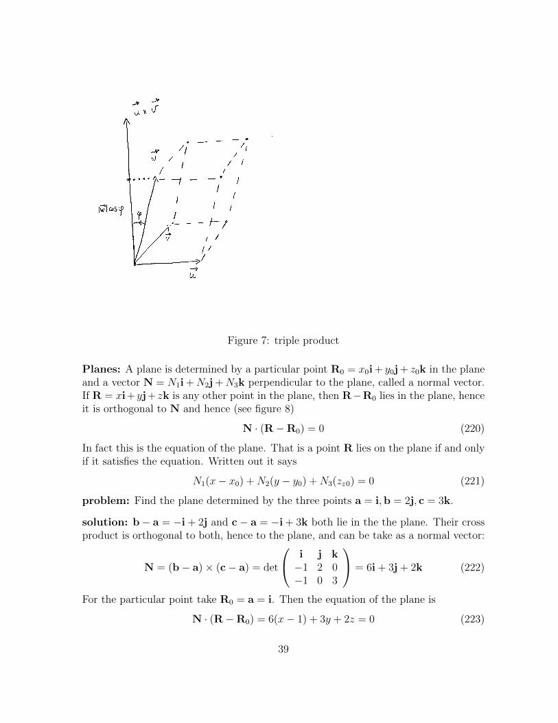
Figure 7: triple product
Planes: A plane is determined by a particular point R0 = x0i + y0j + z0k in the planeand a vector N = N1i +N2j +N3k perpendicular to the plane, called a normal vector.If R = xi+yj+ zk is any other point in the plane, then R−R0 lies in the plane, henceit is orthogonal to N and hence (see figure 8)
N · (R−R0) = 0 (220)
In fact this is the equation of the plane. That is a point R lies on the plane if and onlyif it satisfies the equation. Written out it says
N1(x− x0) +N2(y − y0) +N3(zz0) = 0 (221)
problem: Find the plane determined by the three points a = i,b = 2j, c = 3k.
solution: b− a = −i + 2j and c− a = −i + 3k both lie in the the plane. Their crossproduct is orthogonal to both, hence to the plane, and can be take as a normal vector:
N = (b− a)× (c− a) = det
i j k−1 2 0−1 0 3
= 6i + 3j + 2k (222)
For the particular point take R0 = a = i. Then the equation of the plane is
N · (R−R0) = 6(x− 1) + 3y + 2z = 0 (223)
39

Figure 8:
2.2 vector-valued functions
A vector-valued function is a function from R to R3 (or more generally Rn). It is written
R(t) = (x(t), y(t), z(t)) = x(t)i + y(t)j + z(t)k (224)
To say R(t) has limitlimt→t0
R(t) = R0 (225)
means thatlimt→t0|R(t)−R0| = 0 (226)
If R0 = x0i + y0j + z0j then
|R(t)−R0| =√
(x(t)− x0)2 + (y(t)− y0)2 + (z(t)− z0)2 (227)
Hence limt→t0 R(t) = R0 is the same as the three limits
limt→t0
x(t) = x0 limt→t0
y(t) = y0 limt→t0
z(t) = z0 (228)
The function R(t) is continuous if
limt→t0
R(t) = R0 (229)
40

Figure 9: tangent vector to a curve
This is the same as saying that the components x(t), y(t), z(t) are all continuous.The function R(t) is differentiable if
R′(t) =dR
dt= lim
h→0
R(t+ h)−R(t)
h(230)
exists. Since
R(t+ h)−R(t)
h=x(t+ h)− x(t)
hi +
y(t+ h)− y(t)
hj +
z(t+ h)− z(t)
hk (231)
this is the same as saying that the components x(t), y(t), z(t) are all differentiable, inwhich case the derivative is
R′(t) = x′(t)i + y′(t)j + z′(t)k (232)
41
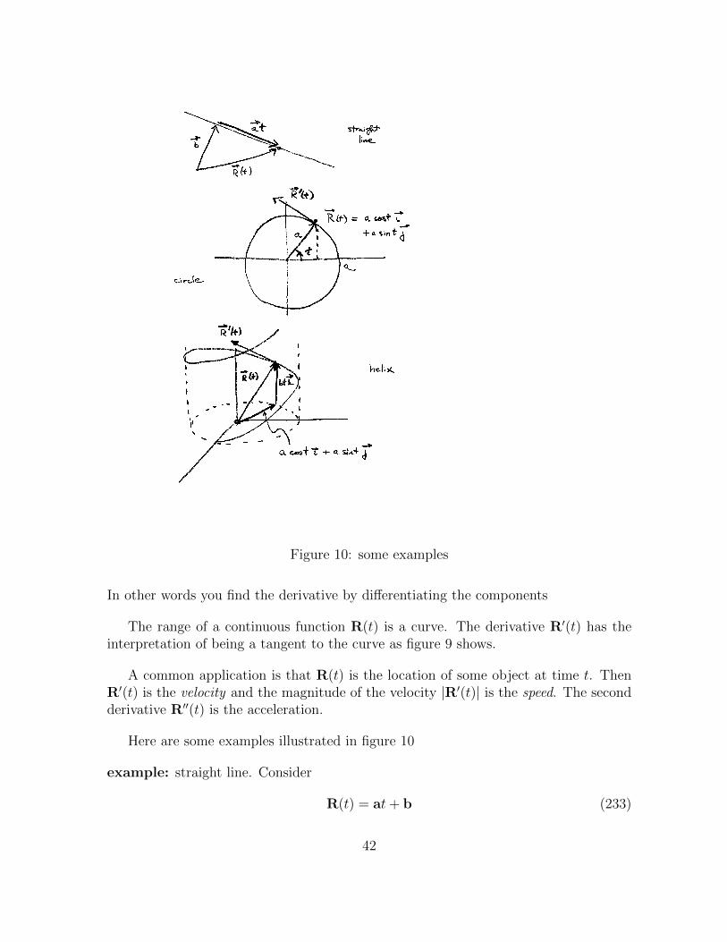
Figure 10: some examples
In other words you find the derivative by differentiating the components
The range of a continuous function R(t) is a curve. The derivative R′(t) has theinterpretation of being a tangent to the curve as figure 9 shows.
A common application is that R(t) is the location of some object at time t. ThenR′(t) is the velocity and the magnitude of the velocity |R′(t)| is the speed. The secondderivative R′′(t) is the acceleration.
Here are some examples illustrated in figure 10
example: straight line. Consider
R(t) = at+ b (233)
42

Then R(0) = b and R′(t) = a so it is a straight line through b in the direction a.
example: circle. Let R(t) be the point on a circle of radius a with polar angle t.As t increases it travels around the circle at uniform speed. The point has Cartesiancoordinates x = a cos t, y = a sin t so
R(t) = a cos t i + a sin t j (234)
The velocity isR′(t) = −a sin t i + a cos t j (235)
and the speed is |R′| = a.
example: helix. To the previous example we add a constant velocity in the z-direction
R(t) = a cos t i + a sin t j + btk (236)
This describes a helix and we have
R′(t) = −a sin t i + a cos t j + bk (237)
2.3 other coordinate systems
We next describe vector valued functions using other coordinate systems.
A. Polar: First some general remarks about vectors and polar coordinates in R2.Let R(r, θ) be the point with polar coordinates r, θ. This has Cartesian coordinatesx = r cos θ, y = r sin θ so
R(r, θ) = r cos θi + r sin θj (238)
If we vary r with θ fixed we get an ”r-line”. The tangent vector to this line is
∂R
∂r(r, θ) = cos θi + sin θj (239)
If we vary θ with r fixed we get an ”θ-line”. The tangent vector to this line is
∂R
∂θ(r, θ) = −r sin θi + r cos θj (240)
We also consider unit tangent vectors to these coordinate lines:
er(θ) =∂R/∂r
|∂R/∂r|= cos θi + sin θj
eθ(θ) =∂R/∂θ
|∂R/∂θ|= − sin θi + cos θj
(241)
See figure 11.
43
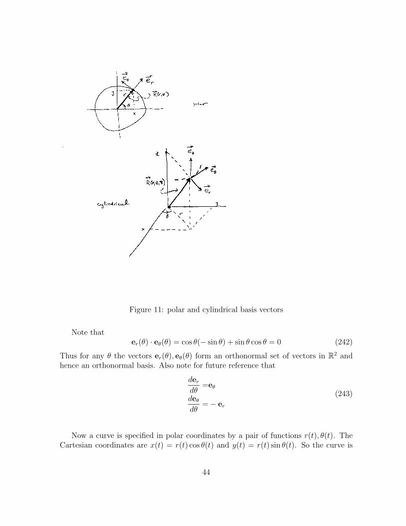
Figure 11: polar and cylindrical basis vectors
Note thater(θ) · eθ(θ) = cos θ(− sin θ) + sin θ cos θ = 0 (242)
Thus for any θ the vectors er(θ), eθ(θ) form an orthonormal set of vectors in R2 andhence an orthonormal basis. Also note for future reference that
derdθ
=eθ
deθdθ
=− er
(243)
Now a curve is specified in polar coordinates by a pair of functions r(t), θ(t). TheCartesian coordinates are x(t) = r(t) cos θ(t) and y(t) = r(t) sin θ(t). So the curve is
44
described in polar coordinates with polar basis vectors by
R(t) =x(t)i + y(t)j
=r(t)(cos θ(t)i + sin θ(t)j)
=r(t)er(θ(t))
(244)
The velocity is
R′(t) = r′(t)er(θ(t)) + r(t)d
dter(θ(t)) (245)
Butd
dter(θ(t)) =
derdθ
(θ(t))dθ
dt= θ′(t)eθ(θ(t)) (246)
and soR′(t) = r′(t)er(θ(t)) + r(t)θ′(t)eθ(θ(t)) (247)
By differentiating this we get a formula for the acceleration R′′(t):
R′′(t) =(r′′(t)− r′(t)(θ′(t))2
)er(θ(t)) +
(r(t)θ′′(t) + 2r′(t)θ′(t)
)eθ(θ(t)) (248)
We summarize in an abbreviated notation
R =rer
R′ =r′er + rθ′eθ
R′′ =(r′′ − r(θ′)2)er + (rθ′′ + 2r′θ′)eθ
(249)
example: Consider the spiral described in polar coordinates by r = at and θ = bt.Then r′ = a, θ′ = b and r′′ = 0, θ′′ = 0 and so
R =at er
R′ =a er + abt eθ
R′′ =− ab2t er + 2ab eθ
(250)
In these formulas er = er(bt) = cos(bt)i+sin(bt)j and eθ = eθ(bt) = − sin(bt)i+cos(bt)j.
B. cylindrical: Cylindrical coordinates in R3 replace x, y by polar coordinates r, θ andleave z alone. Thus
x =r cos θ
y =r sin θ
z =z
(251)
A point with cylindrical coordinates r, θ, z is
R(r, θ, z) = r cos θ i + r sin θ j + z k (252)
45

Unit tangent vectors to the coordinate lines are er, eθ as before and ez = k. See figure11.
A curve in cylindrical coordinate is given by r(t), θ(t), z(t) and we have
R(t) = r(t)er(θ(t)) + z(t)ez (253)
As before:
R =rer + zez
R′ =r′er + rθ′eθ + z′ez
R′′ =(r′′ − r(θ′)2)er + (rθ′′ + 2r′θ′)eθ + z′′ez
(254)
C. spherical: Spherical coordinates ρ, φ, θ label a point by its distance to the origin,the angle with the z-axis, and the polar angle when projected into the x, y plane. Thecorresponding Cartesian coordinates are
x =ρ sinφ cos θ
y =ρ sinφ sin θ
z =ρ cosφ
(255)
The point with spherical coordinates ρ, φ, θ is
R(ρ, φ, θ) = ρ sinφ cos θ i + ρ sinφ sin θ j + ρ cosφ k (256)
Tangent vectors to the coordinate lines are
∂R
∂ρ= sinφ cos θ i + sinφ sin θ j + cosφ k
∂R
∂φ=ρ cosφ cos θ i + ρ cosφ sin θ j− ρ sinφ k
∂R
∂θ=− ρ sinφ sin θ i + ρ sinφ cos θ j
(257)
Divide by the length and get unit tangent vectors to the coordinate lines: (see figure12)
eρ(φ, θ) = sinφ cos θ i + sinφ sin θ j + cosφ k
eφ(φ, θ) = cosφ cos θ i + cosφ sin θ j− sinφ k
eθ(φ, θ) =− sin θ i + cos θ j
(258)
A curve is spherical coordinates is specified by three functions r(t), φ(t), θ(t). Thecorresponding vector-valued function is
R(t) =x(t)i + y(t)j + z(t)k
=ρ(t)(
sinφ(t) cos θ(t)i + sinφ(t) sin θ(t)j + cosφ(t)k)
=ρ(t)eρ(φ(t), θ(t))
(259)
46
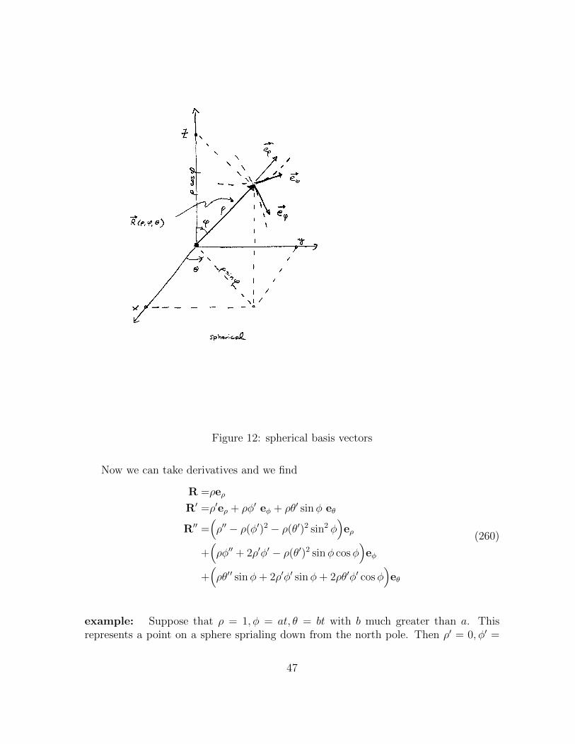
Figure 12: spherical basis vectors
Now we can take derivatives and we find
R =ρeρ
R′ =ρ′eρ + ρφ′ eφ + ρθ′ sinφ eθ
R′′ =(ρ′′ − ρ(φ′)2 − ρ(θ′)2 sin2 φ
)eρ
+(ρφ′′ + 2ρ′φ′ − ρ(θ′)2 sinφ cosφ
)eφ
+(ρθ′′ sinφ+ 2ρ′φ′ sinφ+ 2ρθ′φ′ cosφ
)eθ
(260)
example: Suppose that ρ = 1, φ = at, θ = bt with b much greater than a. Thisrepresents a point on a sphere sprialing down from the north pole. Then ρ′ = 0, φ′ =
47

a, θ′ = b and ρ′′ = 0, φ′′ = 0, θ′′ = 0 and we have with eρ = eρ(at, bt), etc
R =eρ
R′ =a eφ + b sin at eθ
R′′ =(− a2 − b2 sin2 at
)eρ +
(− b2 sin at cos at
)eφ +
(2ab cos at
)eθ
(261)
2.4 line integrals
We want to define the length of a curve C in R3. Suppose the curve is the range of avector valued function R(t) = x(t)i + y(t)j + z(t)k, a ≤ t ≤ b. We say that R(t) isa parametrization of C. There will be many parametrizations, but we pick one. Wedivide up the interval [a, b] by picking points
a = t0 < t1 < t2 < · · · < tn = b (262)
This gives a sequence of points on the curve R(t0),R(t1), . . .R(tn). (see figure 13). If∆ti = ti+1 − ti is small then for any t∗i in the interval [ti, ti+1]
R(ti+1)−R(ti) = (x(ti+1)− x(ti))i + (y(ti+1)− y(ti))j + (z(ti+1)− z(ti))k
≈ x′(t∗i )∆tii + y′(t∗i )∆tij + z′(t∗i )∆tik
= R′(t∗i )∆ti
(263)
(The mean value theorem says there is a point t∗i so that (x(ti+1)− x(ti)) = x′(t∗i )∆ti.Changing to an arbitrary point in the interval is second order small and negligible).Let ∆si be the length of the straight line from R(ti) to R(ti+1). Then
∆si = |R(ti+1)−R(ti)| ≈ |R′(t∗i )|∆ti (264)
Then we have
length of C ≈n−1∑i=0
∆si ≈n−1∑i=0
|R′(t∗i )|∆ti (265)
This is a Riemann sum and as the division becomes increasingly fine, i.e as maxi ∆titends to 0, this converges a Riemann integral which we take as the definition
length of C =
∫ b
a
|R′(t)|dt (266)
One can show that this depends only on C and not on the particular parametrization.
48

Figure 13: line integral
More generally we want to define the integral of a function f(R) = f(x, y, z) overthe curve C. An approximation to what we want is
n−1∑i=0
f(R(t∗i ))∆si ≈n−1∑i=0
f(R(t∗i ))|R′(t∗i )|∆ti (267)
As the division becomes fine this converges to a Riemann integral which we take as thedefinition of the integral of f over C. It is denoted
∫C f(R)ds and is given by∫
Cf(R)ds =
∫ b
a
f(R(t))|R′(t)|dt (268)
This is also independent of parametrization. A short way to remember it is to replaceR by its parametrization R(t), replace C by the interval [a, b] and replace the formal
49

symbol ds by
ds =
∣∣∣∣dRdt∣∣∣∣ dt (269)
Note also that if f(R) = 1 we have∫Cds = length of C (270)
The same formulas hold in R2 but now R(t) = x(t)i + y(t)j.
example: Consider the helix parametrized by
R(t) = a cos t i + a sin t j + bt k (271)
with 0 ≤ t ≤ 2π. Then
dR
dt= −a sin t i + a cos t j + b k (272)
and
ds =
∣∣∣∣dRdt∣∣∣∣ dt =
√a2 + b2 dt (273)
The length is then ∫Cds =
∫ 2π
0
√a2 + b2 dt = 2π
√a2 + b2 (274)
example: Suppose we have a thin semi-circular wire of radius a with uniform lineardensity ρ (mass per unit of length). We want to find the y-component of the center ofmass. This is defined by dividing the wire up into segments of length ∆si and mass∆mi = ρ∆si and computing
y =
∑i yi∆mi∑i ∆mi
=
∑i yi∆si∑i ∆si
(275)
where yi is the y-coordinate of the ith segment. As the division becomes fine this isexpressed as a ratio of line integrals over the semi-circle C
y =
∫C yds∫C ds
(276)
To compute it parametrize the semi-circle by
R(θ) = a cos θi + a sin θj (277)
50
with 0 ≤ θ ≤ π. ThendR
dθ= −a sin θ i + a cos θ j (278)
and
ds =
∣∣∣∣dRdθ∣∣∣∣ dθ = adθ (279)
Then since y = a sin θ ∫Cy ds =
∫ π
0
a sin θ adθ = 2a2 (280)
and ∫Cds =
∫ π
0
adθ = aπ (281)
Thus
y =2a2
aπ=
2a
π(282)
2.5 double integrals
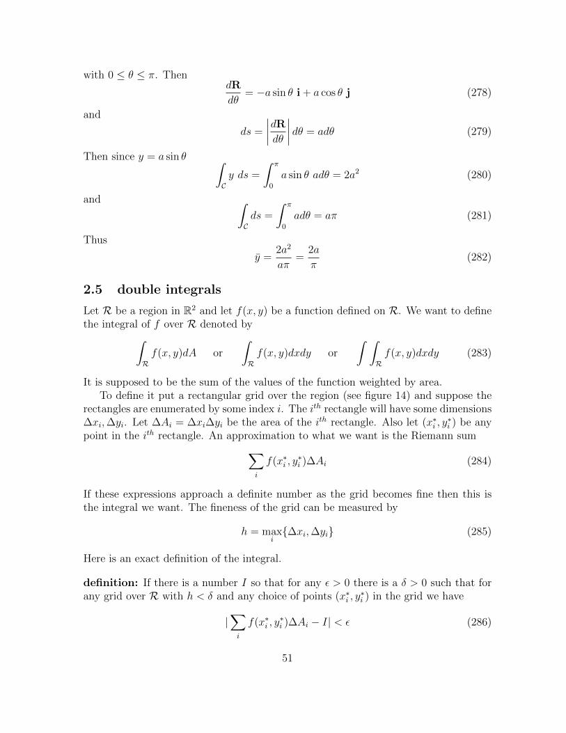
Let R be a region in R2 and let f(x, y) be a function defined on R. We want to definethe integral of f over R denoted by∫
Rf(x, y)dA or
∫Rf(x, y)dxdy or
∫ ∫Rf(x, y)dxdy (283)
It is supposed to be the sum of the values of the function weighted by area.To define it put a rectangular grid over the region (see figure 14) and suppose the
rectangles are enumerated by some index i. The ith rectangle will have some dimensions∆xi,∆yi. Let ∆Ai = ∆xi∆yi be the area of the ith rectangle. Also let (x∗i , y
∗i ) be any
point in the ith rectangle. An approximation to what we want is the Riemann sum∑i
f(x∗i , y∗i )∆Ai (284)
If these expressions approach a definite number as the grid becomes fine then this isthe integral we want. The fineness of the grid can be measured by
h = maxi{∆xi,∆yi} (285)
Here is an exact definition of the integral.
definition: If there is a number I so that for any ε > 0 there is a δ > 0 such that forany grid over R with h < δ and any choice of points (x∗i , y
∗i ) in the grid we have
|∑i
f(x∗i , y∗i )∆Ai − I| < ε (286)
51

Figure 14: double integral
then f is integrable over R and we define∫Rf(x, y)dA = I (287)
For short one can write this as∫Rf(x, y)dA = lim
h→0
∑i
f(x∗i , y∗i )∆Ai (288)
although it is not an ordinary limit since the right side is not a function of h.
One can show:
Theorem 12 Continuous functions are integrable.
Here are some applications of double integrals:
1. With f = 1 ∫RdA = area of R (289)
52

2. If R represents a thin plate and f(x, y) is the density of the plate (mass per unitarea) then f(x∗i , y
∗i )∆Ai is the approximate mass of the ith rectangle and so∫
Rf(x, y)dA = total mass of plate (290)
3. If f(x, y) ≥ 0 then f(x∗i , y∗i )∆Ai is the approximate volume of the column above
the ith rectangle and under the graph and so∫Rf(x, y)dA = volume under the graph of z = f(x, y) above R (291)
Here are some properties of double integrals:
1. For any two functions f1, f2 on R∫R
(f1 + f2)dA =
∫Rf1dA+
∫Rf2dA
2. If α is a constant ∫RαfdA = α
∫RfdA
3. If R can be written as a disjoint union R = R1 ∪R2 then∫RfdA =
∫R1
fdA+
∫R2
fdA
To compute double integrals one writes them as iterated integrals in one variableand then uses the fundamental theorem of calculus.
Theorem 13 Suppose the region R has the form
R = {(x, y) : a ≤ x ≤ b, p(x) ≤ y ≤ q(x)} (292)
for some functions p, q. (See figure 15). Then∫Rf(x, y)dA =
∫ b
a
(∫ q(x)
p(x)
f(x, y)dy)dx (293)
This says fix x and integrate over the y values in the region for this value of x. Thisgives you a function of x which you integrate over the x values for the region.
53

Figure 15: iterated integral
example: Suppose the region R below the graph of y = −x2 + 1 in the first quadrant.Thus R is defined by 0 ≤ x ≤ 1 and 0 ≤ y ≤ −x2 + 1. We compute∫
RxdA =
∫ 1
0
(∫ −x2+1
0
xdy
)dx =
∫ 1
0
[xy]y=−x2+1y=0 dx
=
∫ 1
0
(−x3 + x)dx = −1
4+
1
2=
1
4
(294)
Alternatively R can be regarded as the region 0 ≤ y ≤ 1 and 0 ≤ x ≤√
1− y (draw apicture). Then we can do the x integral first:∫
RxdA =
∫ 1
0
(∫ √1−y
0
xdx
)dy =
∫ 1
0
[x2
2
]x=√
1−y
x=0
dy
=
∫ 1
0
1− y2
dy =1
2− 1
4=
1
4
(295)
54

2.6 triple integrals
Now R be a region in R3 and let f be a function defined on R. We want to define theintegral of f over R which will be denoted∫
Rf(x, y, z)dV or
∫Rf(x, y, z)dxdydz (296)
To defined it divide the region R up into many small rectangular boxes. Suppose theith box has dimensions ∆xi,∆yi,∆zi and volume ∆Vi = ∆xi∆yi∆zi and let (x∗i , y
∗i , z∗i )
be an arbitrary point in the ith box. Also let
h = maxi
(∆xi,∆yi,∆zi) (297)
be the large dimension in the grid. Then we define∫Rf(x, y, z)dV = lim
h→0
∑i
f(x∗i , y∗i , z∗i )∆Vi (298)
If f = 1 then∫R dV is interpreted as the volume of R. Another application is that
R could represent a solid object. If f(x, y, z) is the density at the point (x, y, z) (massper unit volume) then
∫R f(x, y, z)dV is the total mass of the object.
Suppose the regionR is the region between the graphs of z = φ(x, y) and z = ψ(x, y)with (x, y) restricted to some plane region E (see figure 16). Then we can write thetriple integral as a single integral followed by a double integral:∫
Rf(x, y, z)dV =
∫E
(∫ ψ(x,y)
φ(x,y)
f(x, y, z)dz
)dA (299)
If in addition the plane region E is the region between two curves y = p(x) and y = q(x)with a ≤ x ≤ b then the double integral can be written as an iterated in integral andwe have ∫
Rf(x, y, z)dV =
∫ b
a
(∫ q(x)
p(x)
(∫ ψ(x,y)
φ(x,y)
f(x, y, z)dz
)dy
)dx (300)
example: Suppose we are given the problem of finding the volume between theparaboloid z = 2− x2 − y2 and the plane z = 1.
These surfaces intersect when x2 + y2 = 1. The problem must be refering to theregion with x2 + y2 ≤ 1 since the region with x2 + y2 ≥ 1 is infinite. Thus we want tofind the volume of the region R below z = 2−x2−y2 and above z = 1 with x2 +y2 ≤ 1.
55
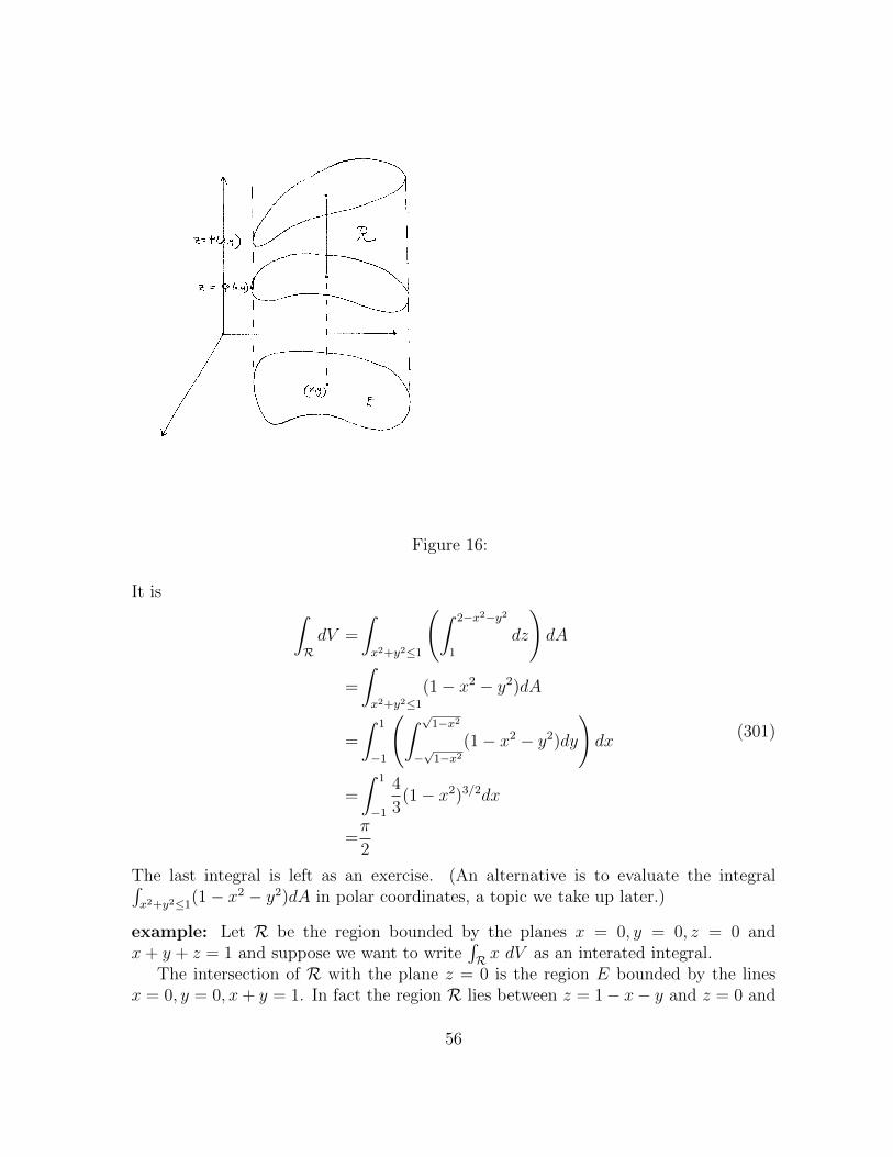
Figure 16:
It is ∫RdV =
∫x2+y2≤1
(∫ 2−x2−y2
1
dz
)dA
=
∫x2+y2≤1
(1− x2 − y2)dA
=
∫ 1
−1
(∫ √1−x2
−√
1−x2(1− x2 − y2)dy
)dx
=
∫ 1
−1
4
3(1− x2)3/2dx
=π
2
(301)
The last integral is left as an exercise. (An alternative is to evaluate the integral∫x2+y2≤1
(1− x2 − y2)dA in polar coordinates, a topic we take up later.)
example: Let R be the region bounded by the planes x = 0, y = 0, z = 0 andx+ y + z = 1 and suppose we want to write
∫R x dV as an interated integral.
The intersection of R with the plane z = 0 is the region E bounded by the linesx = 0, y = 0, x+ y = 1. In fact the region R lies between z = 1− x− y and z = 0 and
56
above E. (draw a picture). Thus we have∫Rx dV =
∫E
(∫ 1−x−y
0
xdz
)(302)
But since E lies between y = 0 and y = 1− x with 0 ≤ x ≤ 1 this can be expressed as∫Rx dV =
∫ 1
0
(∫ 1−x
0
(∫ 1−x−y
0
xdz
)dy
)dx (303)
The evaluation is left as an exercise.
2.7 parametrized surfaces
Consider a function from R ⊂ R2 to R3 which we write as
x = x(u, v) y = y(u, v) z = z(u, v) (304)
The range of this function is a surface S and the function is called a parametrizationof the surface. (A surface has many possible parametrizations, but we pick one). Thefunction can also be written
R(u, v) = x(u, v)i + y(u, v)j + z(u, v)k (305)
example: Consider the function
x =a sinφ cos θ
y =a sinφ sin θ
z =a cosφ
(306)
with 0 < φ < π and 0 < θ < 2π. Then S is the surface of a sphere of radius a, and itis parametrized by spherical coordinates.
example: Suppose S is the graph of a function z = φ(x, y) with (x, y) ∈ R. Then Scan be parametrized by
x = u y = v z = φ(u, v) (307)
with (u, v) ∈ R. This can also be written
x = x y = y z = φ(x, y) (308)
with (x, y) ∈ R.
57

Figure 17:
Now suppose S is a surface parametrized by R(u, v). At (u0, v0) we fix v and varyu we get a u-line in S. Then
∂R
∂u(u0, v0) = tangent vector to u-line through R(u0, v0)
∂R
∂v(u0, v0) = tangent vector to v-line through R(u0, v0)
Together these two tangent vectors determine the tangent plane to the surface atR(u0, v0). A normal to this tangent plane is (see figure 17)
N =∂R
∂u(u0, v0)× ∂R
∂v(u0, v0) (309)
With this N the equation of the tangent plane to the surface S at R0 = R(u0, v0) is
N · (R−R0) = 0 (310)
example: Suppose we want to find the tangent plane to the surface
x = u+ v y = u− v z = 2uv (311)
58
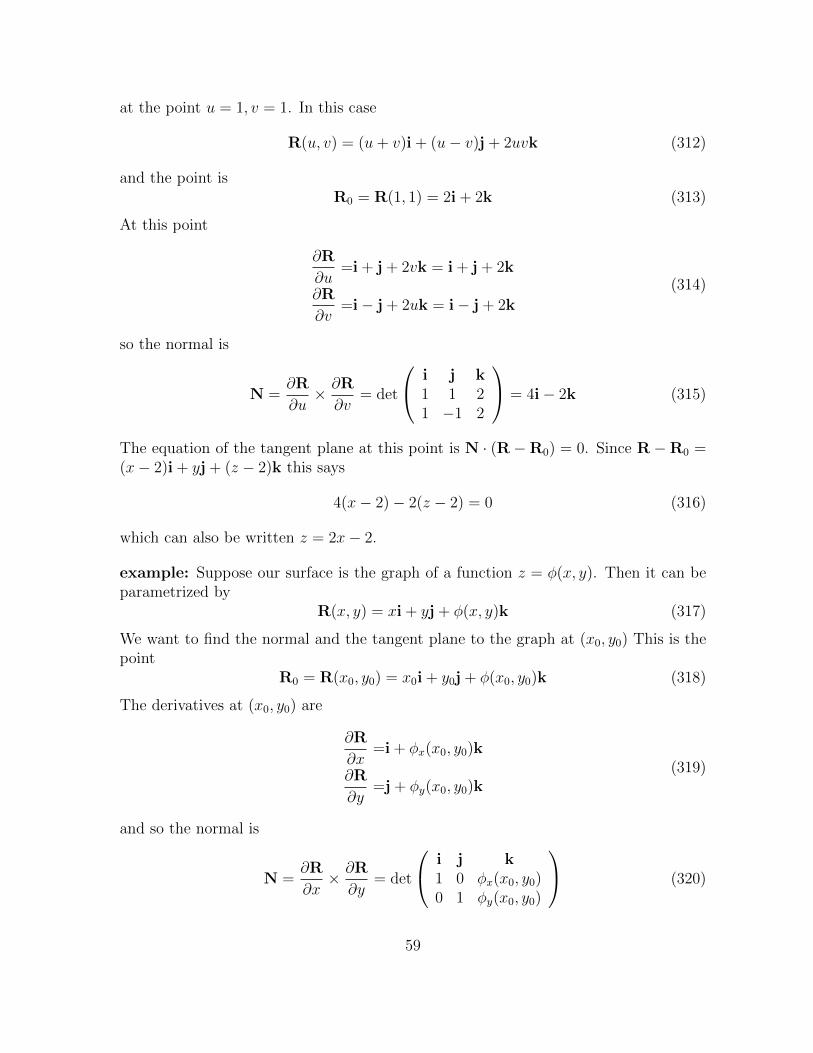
at the point u = 1, v = 1. In this case
R(u, v) = (u+ v)i + (u− v)j + 2uvk (312)
and the point isR0 = R(1, 1) = 2i + 2k (313)
At this point
∂R
∂u=i + j + 2vk = i + j + 2k
∂R
∂v=i− j + 2uk = i− j + 2k
(314)
so the normal is
N =∂R
∂u× ∂R
∂v= det
i j k1 1 21 −1 2
= 4i− 2k (315)
The equation of the tangent plane at this point is N · (R−R0) = 0. Since R−R0 =(x− 2)i + yj + (z − 2)k this says
4(x− 2)− 2(z − 2) = 0 (316)
which can also be written z = 2x− 2.
example: Suppose our surface is the graph of a function z = φ(x, y). Then it can beparametrized by
R(x, y) = xi + yj + φ(x, y)k (317)
We want to find the normal and the tangent plane to the graph at (x0, y0) This is thepoint
R0 = R(x0, y0) = x0i + y0j + φ(x0, y0)k (318)
The derivatives at (x0, y0) are
∂R
∂x=i + φx(x0, y0)k
∂R
∂y=j + φy(x0, y0)k
(319)
and so the normal is
N =∂R
∂x× ∂R
∂y= det
i j k1 0 φx(x0, y0)0 1 φy(x0, y0)
(320)
59
which saysN = −φx(x0, y0)i− φy(x0, y0)j + k (321)
The equation of the tangent plane N · (R−R0) = 0 is then
−φx(x0, y0)(x− x0)− φy(x0, y0)(y − y0) + (z − φ(x0, y0)) = 0 (322)
This can also be written
z = φ(x0, y0) + φx(x0, y0)(x− x0) + φy(x0, y0)(y − y0) (323)
which agrees with our earlier definition of the tangent plane.
2.8 surface area
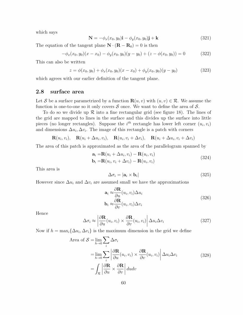
Let S be a surface parametrized by a function R(u, v) with (u, v) ∈ R. We assume thefunction is one-to-one so it only covers S once. We want to define the area of S.
To do so we divide up R into a fine rectangular grid (see figure 18). The lines ofthe grid are mapped to lines in the surface and this divides up the surface into littlepieces (no longer rectangles). Suppose the ith rectangle has lower left corner (ui, vi)and dimensions ∆ui,∆vi. The image of this rectangle is a patch with corners
R(ui, vi), R(ui + ∆ui, vi), R(ui, vi + ∆vi), R(ui + ∆ui, vi + ∆vi)
The area of this patch is approximated as the area of the parallelogram spanned by
ai =R(ui + ∆ui, vi)−R(ui, vi)
bi =R(ui, vi + ∆vi)−R(ui, vi)(324)
This area is∆σi = |ai × bi| (325)
However since ∆ui and ∆vi are assumed small we have the approximations
ai ≈∂R
∂u(ui, vi)∆ui
bi ≈∂R
∂v(ui, vi)∆vi
(326)
Hence
∆σi ≈∣∣∣∣∂R
∂u(ui, vi)×
∂R
∂v(ui, vi)
∣∣∣∣∆ui∆vi (327)
Now if h = maxi{∆ui,∆vi} is the maximum dimension in the grid we define
Area of S = limh→0
∑i
∆σi
= limh→0
∑i
∣∣∣∣∂R
∂u(ui, vi)×
∂R
∂v(ui, vi)
∣∣∣∣∆ui∆vi=
∫R
∣∣∣∣∂R
∂u× ∂R
∂v
∣∣∣∣ dudv(328)
60
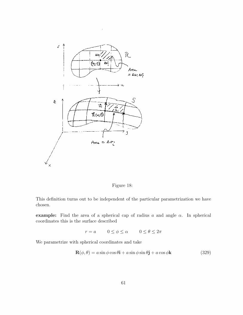
Figure 18:
This definition turns out to be independent of the particular parametrization we havechosen.
example: Find the area of a spherical cap of radius a and angle α. In sphericalcoordinates this is the surface described
r = a 0 ≤ φ ≤ α 0 ≤ θ ≤ 2π
We parametrize with spherical coordinates and take
R(φ, θ) = a sinφ cos θi + a sinφ sin θj + a cosφk (329)
61

with 0 ≤ φ ≤ α, 0 ≤ θ ≤ 2π. Then we compute
∂R
∂φ× ∂R
∂θ= det
i j ka cosφ cos θ a cosφ sin θ −a sinφ−a sinφ sin θ a sinφ cos θ 0
=a2 sin2 φ cos θi + a2 sin2 φ sin θj + a2 cosφ sinφk
(330)
Then ∣∣∣∣∂R
∂φ× ∂R
∂θ
∣∣∣∣ =√a4 sin4 φ(cos2 θ + sin2 θ) + a4 cos2 φ sin2 φ
=a2 sinφ
√sin2 φ+ cos2 φ
=a2 sinφ
(331)
and the area is
Area =
∫ 2π
0
∫ α
0
∣∣∣∣∂R
∂φ× ∂R
∂θ
∣∣∣∣ dφ dθ=
∫ 2π
0
∫ α
0
a2 sinφ dφ dθ
=a2(∫ 2π
0
dθ)(∫ α
0
sinφ dφ)
=2πa2(1− cosα)
(332)
Note that if α = π the area is 4πa2 which is what we expect for the whole sphere.
2.9 surface integrals
We continue to consider a surface S parametrized by a function R(u, v) with (u, v) ∈ R.Also let f(R) = f(x, y, z) be a function defined on S (and possibly elsewhere in R3).We want to define the integral of f over S which will be written
∫S f(R)dσ.
To define it we again divide up the parameter space into a rectangular grid. Wealso let (ui, vi) be the corner point in the ith rectangle. (see figure 18 again). Then wedefine ∫
Sf(R)dσ = lim
h→0
∑i
f(R(ui, vi)
)∆σi
= limh→0
∑i
f(R(ui, vi)
) ∣∣∣∣∂R
∂u(ui, vi)×
∂R
∂v(ui, vi)
∣∣∣∣∆ui∆vi=
∫Rf(R(u, v)
) ∣∣∣∣∂R
∂u× ∂R
∂v
∣∣∣∣ du dv(333)
62

For short one just has to remember
dσ =
∣∣∣∣∂R
∂u× ∂R
∂v
∣∣∣∣ du dv (334)
A special case is with f(R) = 1 which gives∫Sdσ =
∫R
∣∣∣∣∂R
∂u× ∂R
∂v
∣∣∣∣ du dv = Area of S (335)
example: Let S represent a thin hemispherical shell of uniform density which hasradius a and is centered on the orgin. We want to find the z-component of the centerof mass. Since it is a thin shell it is reasonable to represent in terms of surface integralsand we take the definition
z =
∫S z dσ∫S dσ
(336)
The hemisphere is parametrized as before by x = a sinφ cos θ, y = a sinφ sin θ, andz = cosφ with 0 ≤ φ ≤ π/2 and 0 ≤ θ ≤ 2π. We also have as before
dσ =
∣∣∣∣∂R
∂φ× ∂R
∂θ
∣∣∣∣ dφ dθ = a2 sinφ dφ dθ (337)
Then we can compute∫Sz dσ =
∫ 2π
0
∫ π/2
0
(a cosφ)a2 sinφ dφ dθ
=a3(∫ 2π
0
dθ)(∫ π/2
0
cosφ sinφ dφ)
=a3 · 2π · 1
2=πa3
(338)
From our earlier calculation of area we have∫Sdσ = 2πa2 (339)
Thus
z =πa3
2πa2=a
2(340)
example: Suppose that the surface S is the graph of a function z = φ(x, y) with(x, y) ∈ R. As noted previously we can parametrize S by
R(x, y) = xi + yj + φ(x, y)k (x, y) ∈ R (341)
63

We also computed earlier
∂R
∂x× ∂R
∂y= −φxi− φyj + k (342)
Therefore
dσ =
∣∣∣∣∂R
∂x× ∂R
∂y
∣∣∣∣ dxdy =√
1 + φ2x + φ2
y dxdy (343)
and so ∫Sf(x, y, z)dσ =
∫Rf(x, y, φ(x, y))
√1 + φ2
x + φ2y dxdy (344)
In particular
Area of S =
∫Sdσ =
∫R
√1 + φ2
x + φ2y dxdy (345)
2.10 change of variables in R2
Consider a special case of the surface integral in which the surface S lies in the xy plane.Then the parametrization has the form x = x(u, v), y = y(u, v), z = 0 for (u, v) ∈ R.In vector form
R(u, v) = x(u, v)i + y(u, v)j (346)
In this case
∂R
∂u× ∂R
∂v= det
i j kxu yu 0xv yv 0
= det
(xu yuxv yv
)k
= det
(xu xvyu yv
)k =
∂(x, y)
∂(u, v)k
(347)
and so
dσ =
∣∣∣∣∂R
∂u× ∂R
∂v
∣∣∣∣ dudv =
∣∣∣∣∂(x, y)
∂(u, v)
∣∣∣∣ dudv (348)
Then our surface integral is evaluated as∫Sf(x, y)dσ =
∫Rf(x(u, v), y(u, v))
∣∣∣∣∂(x, y)
∂(u, v)
∣∣∣∣ dudv (349)
However since S is flat the surface integral∫S f(x, y)dσ is the same as the area integral∫
S f(x, y)dA. It has been divided up in an irregular fashion but the result is the same.Thus we have demonstrated the following change of variables formula:
Theorem 14 Let a region S ⊂ R2 be the image of a region R ⊂ R2 under a differen-tiable invertible function x = x(u, v), y = y(u, v). Then∫
Sf(x, y)dA =
∫Rf(x(u, v), y(u, v))
∣∣∣∣∂(x, y)
∂(u, v)
∣∣∣∣ dudv (350)
64

One can think of (u, v) as new coordinates for the region S. Then a short versionof the theorem is
dA =
∣∣∣∣∂(x, y)
∂(u, v)
∣∣∣∣ dudv (351)
expressing the area element in the new coordinates.
As a special case consider polar coordinates x = r cos θ, y = r sin θ. Then
∂(x, y)
∂(r, θ)= det
(xr xθyr yθ
)= det
(cos θ −r sin θsin θ r cos θ
)= r (352)
and so dA = rdrdθ. The change of variables formula is∫Sf(x, y) dA =
∫Rf(r cos θ, r sin θ) rdrdθ (353)
Here R is all points (r, θ) such that (x, y) = (r cos θ, r sin θ) is in S. Thus R is just Sdescribed in polar coordinates.
example: Suppose S is the half-disc x2 + y2 ≤ 4, y > 0 and we want to evaluate∫S(3− x2 − y2)dA (354)
In polar coordinates S becomes the region R defined by 0 < r < 2, 0 < θ < π. Thus∫S(3− x2 − y2)dA =
∫R
(3− r2)rdrdθ
=
∫ π
0
∫ 2
0
(3r − r3)drdθ
=π
[3r2
2− r4
4
]2
0
=2π
(355)
example: Let S be the region bounded by the lines x + y = −1, x + y = 3, 2x − y =0, 2x− y = 4. (see figure 19) We want to evaluate the integral∫
S(x+ y)dA (356)
We make a change of variables suggested by the boundary lines and set
u =x+ y
v =2x− y(357)
65
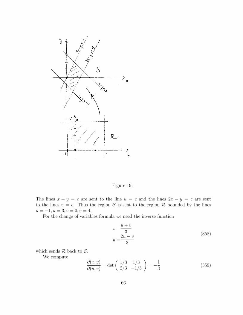
Figure 19:
The lines x + y = c are sent to the line u = c and the lines 2x − y = c are sentto the lines v = c. Thus the region S is sent to the region R bounded by the linesu = −1, u = 3, v = 0, v = 4.
For the change of variables formula we need the inverse function
x =u+ v
3
y =2u− v
3
(358)
which sends R back to S.We compute
∂(x, y)
∂(u, v)= det
(1/3 1/32/3 −1/3
)= −1
3(359)
66
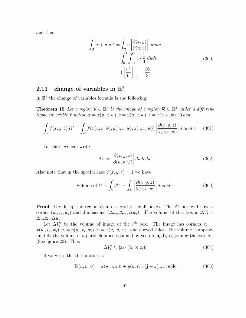
and then ∫S(x+ y)dA =
∫Ru
∣∣∣∣∂(x, y)
∂(u, v)
∣∣∣∣ dudv=
∫ 4
0
∫ 3
−1
u · 1
3dudv
=4
[u2
6
]3
−1
=16
3
(360)
2.11 change of variables in R3
In R3 the change of variables formula is the following:
Theorem 15 Let a region V ⊂ R3 be the image of a region R ⊂ R3 under a differen-tiable invertible function x = x(u, v, w), y = y(u, v, w), z = z(u, v, w). Then∫
Vf(x, y, z)dV =
∫Rf(x(u, v, w), y(u, v, w), z(u, v, w))
∣∣∣∣ ∂(x, y, z)
∂(u, v, w)
∣∣∣∣ dudvdw (361)
For short we can write
dV =
∣∣∣∣ ∂(x, y, z)
∂(u, v, w)
∣∣∣∣ dudvdw (362)
Also note that in the special case f(x, y, z) = 1 we have
Volume of V =
∫VdV =
∫R
∣∣∣∣ ∂(x, y, z)
∂(u, v, w)
∣∣∣∣ dudvdw (363)
Proof. Divide up the region R into a grid of small boxes. The ith box will have acorner (ui, vi, wi) and dimensions (∆ui,∆vi,∆wi). The volume of this box is ∆Vi =∆ui∆vi∆wi.
Let ∆V ′i be the volume of image of the ith box. The image has corners xi =x(ui, vi, wi), yi = y(ui, vi, wi), zi = z(ui, vi, wi) and curved sides. The volume is approx-imately the volume of a parallelopiped spanned by vectors ai,bi, ci joining the corners.(See figure 20). Thus
∆V ′i ≈ |ai · (bi × ci)| (364)
If we write the the funtion as
R(u, v, w) = x(u, v, w)i + y(u, v, w)j + z(u, v, w)k (365)
67
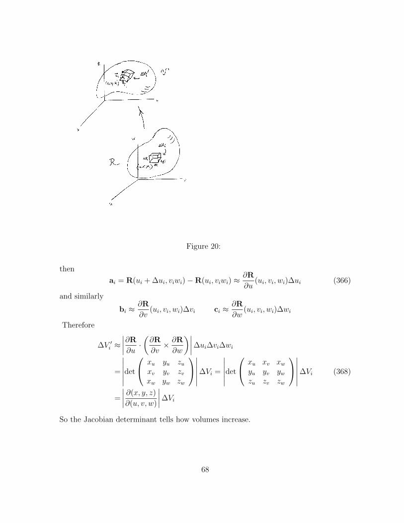
Figure 20:
then
ai = R(ui + ∆ui, viwi)−R(ui, viwi) ≈∂R
∂u(ui, vi, wi)∆ui (366)
and similarly
bi ≈∂R
∂v(ui, vi, wi)∆vi ci ≈
∂R
∂w(ui, vi, wi)∆wi
Therefore
∆V ′i ≈∣∣∣∣∂R
∂u·(∂R
∂v× ∂R
∂w
)∣∣∣∣∆ui∆vi∆wi=
∣∣∣∣∣∣det
xu yu zuxv yv zvxw yw zw
∣∣∣∣∣∣∆Vi =
∣∣∣∣∣∣det
xu xv xwyu yv ywzu zv zw
∣∣∣∣∣∣∆Vi=
∣∣∣∣ ∂(x, y, z)
∂(u, v, w)
∣∣∣∣∆Vi(368)
So the Jacobian determinant tells how volumes increase.
68
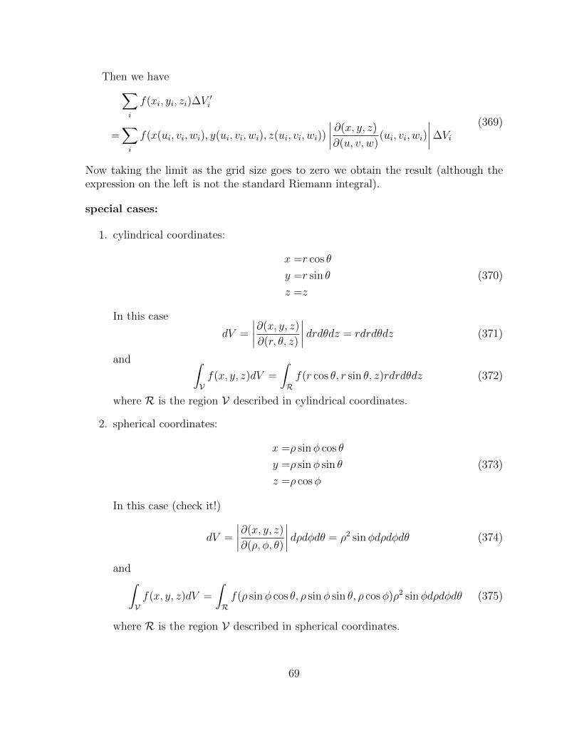
Then we have∑i
f(xi, yi, zi)∆V′i
=∑i
f(x(ui, vi, wi), y(ui, vi, wi), z(ui, vi, wi))
∣∣∣∣ ∂(x, y, z)
∂(u, v, w)(ui, vi, wi)
∣∣∣∣∆Vi (369)
Now taking the limit as the grid size goes to zero we obtain the result (although theexpression on the left is not the standard Riemann integral).
special cases:
1. cylindrical coordinates:
x =r cos θ
y =r sin θ
z =z
(370)
In this case
dV =
∣∣∣∣∂(x, y, z)
∂(r, θ, z)
∣∣∣∣ drdθdz = rdrdθdz (371)
and ∫Vf(x, y, z)dV =
∫Rf(r cos θ, r sin θ, z)rdrdθdz (372)
where R is the region V described in cylindrical coordinates.
2. spherical coordinates:
x =ρ sinφ cos θ
y =ρ sinφ sin θ
z =ρ cosφ
(373)
In this case (check it!)
dV =
∣∣∣∣∂(x, y, z)
∂(ρ, φ, θ)
∣∣∣∣ dρdφdθ = ρ2 sinφdρdφdθ (374)
and∫Vf(x, y, z)dV =
∫Rf(ρ sinφ cos θ, ρ sinφ sin θ, ρ cosφ)ρ2 sinφdρdφdθ (375)
where R is the region V described in spherical coordinates.
69
example: Suppose we want to find the volume of the quarter-cone in a sphere V whichis described in spherical coordinates by 0 < ρ < 1, 0 < φ < π/4, 0 < θ < π/2. Wecompute
Volume =
∫VdV
=
∫ π/2
0
∫ π/4
0
∫ 1
0
ρ2 sinφ dρ dφ dθ
=(∫ 1
0
ρ2dρ)(∫ π/4
0
sinφ dφ)(∫ π/2
0
dθ)
=1
3·[− cosφ
]π/40· π/2
=π
6
(1− 1√
2
)(376)
2.12 derivatives in R3
In R3 we continue to use the notation
R = xi + yj + zk = (x, y, z) (377)
A scalar is a function from R3 to R and has the form
u = u(R) = u(x, y, z) (378)
A scalar can be drawn (not very well) by shading points in R3 proportional to the valueof u at that point. Examples of quantites that can be represented by scalars are densityand temperature.
A vector field is function from R3 to R3 and has the form
v = v(R) =v1(R)i + v2(R)j + v3(R)k
=v1(x, y, z)i + v2(x, y, z)j + v3(x, y, z)k(379)
A vector field can be repesented by drawing a vector v(R) at the point R for somerepresentative points R. Examples of quantites that can be represented by scalars areforces and the velocity of a fluid.
We want to define various derivatives of scalars and vector fields. These are specifiedwith the operator
∇ = i∂
∂x+ j
∂
∂y+ k
∂
∂z(380)
which is called del or nabla. If u is a scalar we define a vector field
gradient of u = ∇u = i∂u
∂x+ j
∂u
∂y+ k
∂u
∂z(381)
70
If v = v1i + v2j + v3k is a vector field we define a scalar
divergence of v = ∇ · v =∂v1
∂x+∂v2
∂y+∂v3
∂z(382)
and also a vector field
curl of v =∇× v
= det
i j k∂/∂x ∂/∂y ∂/∂zv1 v2 v3
=i
(∂v3
∂y− ∂v2
∂z
)+ j
(∂v1
∂z− ∂v3
∂x
)+ k
(∂v2
∂x− ∂v1
∂y
) (383)
Finally if u is a scalar we define
Laplacian of u = ∆u = ∇ · ∇u =∂2u
∂x2+∂2u
∂y2+∂2u
∂z2(384)
example: If u = x2 + xy + y2 + yz + z2 + zx then
∇u =(2x+ y + z)i + (2y + x+ z)j + (2z + z + y)k
∆u =∇ · ∇u = 2 + 2 + 2 = 6(385)
example: If v = yz2i + xz2j + (2xyz + z)k then
∇ · v =2xy + 1
∇× v = det
i j k∂/∂x ∂/∂y ∂/∂zyz2 xz2 (2xyz + z)
=(2xz − 2xz)i + (2zy − 2zy)j + (z2 − z2)k = 0
(386)
The derivatives satisfy various identities some of which we list. These hold for anyscalar u and any vector field v, assuming only they are twice continuously differentiable.
1. ∇×∇u = 0
2. ∇ · (∇× v) = 0
3. ∇ · (uv) = ∇u · v + u(∇ · v)
4. ∇ · (v ×w) = (∇× v) ·w − v · (∇×w)
71
5. ∇× (uv) = u(∇× v) +∇u× v
6. ∇× (∇× v) = ∇(∇ · v)−∆v where ∆v = ∆v1i + ∆v2j + ∆v3k
proof of (1.). We compute
∇×∇u = det
i j k∂/∂x ∂/∂y ∂/∂z∂u/∂x ∂u/∂y ∂u/∂z
=( ∂2u
∂y∂z− ∂2u
∂z∂y
)i +( ∂2u
∂z∂x− ∂2u
∂x∂z
)j +( ∂2u
∂x∂y− ∂2u
∂y∂x
)k
=0
(387)
We also note that the chain rule
d
dtu(x(t), y(t), z(t)
)=∂u
∂x
(x(t), y(t), z(t)
)dxdt
+∂u
∂y
(x(t), y(t), z(t)
)dydt
+∂u
∂z
(x(t), y(t), z(t)
)dzdt
(388)
can be written in a vector notation as
d
dtu(R(t)) = ∇u(R(t)) · dR
dt(389)
2.13 gradient
One of our goals is to interpret the gradient, divergence, and curl. Here we give threeinterpretations of the gradient.
1. (∇u)(R0) is normal to the level surface u = constant through R0, i.e the surfaceu(R) = u(R0).
To see this let R(t) be any curve in the surface with R(0) = R0. Thus
u(R(t)) = u(R0) (390)
Taking the derivative with respect to t and using the chain rule gives
(∇u)(R(t)) ·R′(t) = 0 (391)
At t = 0 this says(∇u)(R0) ·R′(0) = 0 (392)
Any tangent vector to the surface at R0 has the form R′(0) for some curve throughR0. Thus (∇u)(R0) is normal to any tangent vector at R0 and hence is normalto the surface. See figure 21.
72

Figure 21:
2. If n is a unit vector, then (∇u)(R0) · n is the rate of change of u at R0 in thedirection n, also called the directional derivative.
To see this use the chain rule to calculate the rate of change as
d
dtu(R0 + tn)
∣∣∣t=0
= (∇u)(R0 + tn) · ddt
(R0 + tn)∣∣∣t=0
= (∇u)(R0) · n (393)
3. (∇u)(R0) is the direction of greatest increase for u at R0.
To see this consider that the direction of greatest increase is the unit vector nwhich maximizes the directional derivative (∇u)(R0) · n. This occurs when n isparallel to (∇u)(R0).
problem Find the normal to the surface which is the graph of z = f(x, y)
solution The surface is
u(x, y, z) = −f(x, y) + z = 0 (394)
73

A normal is∇u = uxi + uyj + uzk = −fxi− fyj + k (395)
as before.
problem Find the direction of greatest change for u = x2 + 2xy + y2 + 3z2 at thepoint (1, 1, 1), i.e. find a unit vector.
solution The gradient at this point is
∇u = (2x+ 2y)i + (2x+ 2y)j + 6zk = 4i + 4j + 6k (396)
A unit vector in this direction is
n =∇u|∇u|
=4i + 4j + 6k√
68(397)
2.14 divergence theorem
The divergence is important because it appears in the following theorem.
Theorem 16 (Divergence Theorem). Let R be a solid region in R3 with boundary sur-face S. Let n be the unit outward normal on S. Then for any continuously differentiablevector field v on R ∫
R∇ · v dV =
∫S
v · n dσ (398)
Proof. Suppose n = n1i + n2j + n3k. If suffices to show that∫R
∂v1
∂xdV =
∫Sv1n1dσ∫
R
∂v2
∂ydV =
∫Sv2n2 dσ∫
R
∂v3
∂zdV =
∫Sv3n3 dσ
(399)
Then adding them together gives the result.We prove the last, the others are similar. To prove it suppose that R if the region
between the graphs of two functions. It is defined by φ(x, y) ≤ z ≤ ψ(x, y) with with(x, y) in some region E in the plane. Then we have∫
R
∂v3
∂zdV =
∫E
(∫ ψ(x,y)
φ(x,y)
∂v3
∂z
)dxdy
=
∫E
(v3(x, y, ψ(x, y))− v3(x, y, φ(x, y)) dxdy
(400)
74

Figure 22:
We need to show that∫S v3n3 dσ has the same expression. Now S has three parts
S1,S2,S3, see figure 22, and∫Sv3n3 dσ =
∫S1v3n3 dσ +
∫S2v3n3 dσ +
∫S3v3n3 dσ (401)
The surface S1 is the graph of z = ψ(x, y) and a normal vector is N = −ψxi−ψyj+k.This is an upward normal since the third component is positive. On this surface upwardis outward and so the unit outward normal is
n =N
|N|=−ψxi− ψyj + k√
1 + ψ2x + ψ2
y
(402)
Also on S1 we have
dσ =√
1 + ψ2x + ψ2
y dxdy (403)
75

Therefore∫S1v3n3 dσ =
∫E
v3(x, y, ψ(x, y))1√
1 + ψ2x + ψ2
y
√1 + ψ2
x + ψ2y dxdy
=
∫E
v3(x, y, ψ(x, y)) dxdy
(404)
The surface S2 is the graph of z = φ(x, y) and an upward normal vector is N =−φxi− φyj + k. On this surface upward is inward and so the unit outward normal is
n = − N
|N|=φxi + φyj− k√
1 + φ2x + φ2
y
(405)
Also on S2 we have
dσ =√
1 + φ2x + φ2
y dxdy (406)
Therefore∫S2v3n3 dσ =
∫E
v3(x, y, ψ(x, y))−1√
1 + φ2x + φ2
y
√1 + φ2
x + φ2y dxdy
=−∫E
v3(x, y, φ(x, y)) dxdy
(407)
On the surface S3 we have n3 = 0 and so∫S3 v3n3 dσ = 0
Adding the contributions from the three surfaces gives the desired result∫Sv3n3 dσ =
∫E
(v3(x, y, ψ(x, y))− v3(x, y, φ(x, y)) dxdy (408)
The divergence theorem can be used in various ways. Here we just offer a couple ofexamples illustrating what it says.
example Let R be a sphere of radius a with surface S. Check the divergence theoremfor this region and the vector field v(R) = R = xi + yj + zk.
For the volume integral note that ∇ ·R = 3 so∫R∇ · v dV = 3
∫RdV = 3× volume of R = 3
(4
3πa3
)= 4πa3 (409)
On the other hand for a sphere the unit normal to the surface S at R is n = R/|R|.Hence on S we have v · n = R ·R/|R| = |R| = a. Therefore∫
Sv · ndσ = a
∫Sdσ = a area of S = a
(4πa2
)= 4πa3 (410)
76
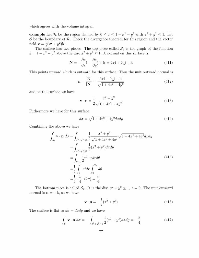
which agrees with the volume integral.
example Let R be the region defined by 0 ≤ z ≤ 1 − x2 − y2 with x2 + y2 ≤ 1. LetS be the boundary of R. Check the divergence theorem for this region and the vectorfield v = 1
2(x2 + y2)k.
The surface has two pieces. The top piece called S1 is the graph of the functionz = 1− x2 − y2 above the disc x2 + y2 ≤ 1. A normal on this surface is
N = −∂z∂x
i− ∂z
∂yj + k = 2xi + 2yj + k (411)
This points upward which is outward for this surface. Thus the unit outward normal is
n =N
|N|=
2xi + 2yj + k√1 + 4x2 + 4y2
(412)
and on the surface we have
v · n =1
2
x2 + y2√1 + 4x2 + 4y2
(413)
Futhermore we have for this surface
dσ =√
1 + 4x2 + 4y2dxdy (414)
Combining the above we have∫S1
v · n dσ =
∫x2+y2≤1
1
2
x2 + y2√1 + 4x2 + 4y2
√1 + 4x2 + 4y2dxdy
=
∫x2+y2≤1
1
2(x2 + y2)dxdy
=
∫r≤1
1
2r2 · rdrdθ
=1
2
∫ 1
0
r3dr
∫ 2π
0
dθ
=1
2· 1
4· (2π) =
π
4
(415)
The bottom piece is called S2. It is the disc x2 + y2 ≤ 1, z = 0. The unit outwardnormal is n = −k, so we have
v · n = −1
2(x2 + y2) (416)
The surface is flat so dσ = dxdy and we have∫S2
v · n dσ = −∫x2+y2≤1
1
2(x2 + y2)dxdy = −π
4(417)
77
Combining the two pieces we have for the surface integral∫S
v · n dσ =
∫S1
v · n dσ +
∫S2
v · n dσ =π
4− π
4= 0 (418)
For the volume integral we note that ∇ · v = ∂/∂z(
(x2 + y2)/2)
= 0 and so∫R∇ · v dV = 0 (419)
which agrees with the surface integral.
remark: In evaluating surface integrals we are frequently canceling awkward squareroots. We can avoid this as follows. If S is a surface with unit normal vector n definea formal symbol d~σ = ndσ and then∫
Sv · n dσ =
∫S
v · d~σ (420)
If S is parametrized by a function R(u, v) then
n =± Ru ×Rv
|Ru ×Rv|dσ =|Ru ×Rv| dudvd~σ =± (Ru ×Rv) dudv
(421)
If S is the graph of a function z = f(x, y) then
n =± −fxi− fyj + k√1 + f 2
x + f 2y
dσ =√
1 + f 2x + f 2
y dxdy
d~σ =± (−fxi− fyj + k) dxdy
(422)
In either case the square roots are gone from d~σ. The only difficulty is that one muststill think about which normal one wants to determine whether to take the plus signor the minus sign.
2.15 applications
We give some applications of the divergence theorem. In the first we answer the question”what is divergence?”. The others are derivations of some basic partial differentialequations.
78

Figure 23:
A. steady fluid fow The steady (i.e. time independent) flow of a fluid is discribedby the following quantities:
v(R) = velocity of the fluid at R (cm/sec)
ρ(R) = density of the fluid at R (gr/cm3)
u(R) = ρ(R)v(R) = mass flow density (gr/cm2 · sec)
Also if S is a surface with unit normal n we define∫S
u · n dσ = flux of u over S in direction n
We want to interpret this flux and also the divergence of u. (They are related).Pick a point R on the the surface S, let ∆σ be a small piece of surface around R.
Then (see figure 23)
mass through ∆σ in time ∆t (gr)
≈ density at R× volume through ∆σ in time ∆t
≈ρ(R)×∆σ × (v(R)∆t) · n=u(R) · n ∆σ∆t
(423)
79

If we divide by ∆t we get
rate of mass flow thru ∆σ = u(R) · n ∆σ (gr/sec)
Now sum over pieces ∆σi covering the surface S and take the limit as the partitionbecomes fine. This gives
rate of mass flow thru S = lim∑i
u(Ri) · ni ∆σi =
∫S
u(R) · n dσ (gr/sec)
Thus we have an interpretation of the flux of u over S. It is the rate of mass flowthrough S.
Now for the divergence of u at any point R let Dε be a sphere of radius ε aroundR. let Sε be the surface of that sphere with outward normal n. Then by the divergencetheorem
(∇ · u)(R) = limε→0
1
Vol Dε
∫Dε
∇ · u dV
= limε→0
1
Vol Dε
(∫Sε
u · n dσ
) (424)
This is the flux divided by the volume. Thus the divergence is the rate of outward massflow per unit volume (gr/ cm3· sec ). A large divergence at a point means a lot of fluidis entering the system at that point.
B. fluid dynamicsAgain we consider fluid flow, but now the velocity v(R, t), the density ρ(R, t), and
the mass flow density u(R, t) = ρ(R, t)v(R, t) all depend on the time t.In our fluid consider any region R with surface S and outward normal n. Conser-
vation of mass says that
rate of mass flow out of S = rate of decrease of mass in R (425)
which means that ∫S
u · n dσ = − d
dt
(∫Rρ(R, t) dV
)(426)
Use the divergence theorem on the left, and differentiate under the integral sign on theright to obtain ∫
R∇ · u dV = −
∫R
∂ρ
∂tdV (427)
which is the same as ∫R
(∇ · u +
∂ρ
∂t
)dV = 0 (428)
80

Since this holds for an arbitrary region R it must be that
∇ · u +∂ρ
∂t= 0 (429)
which is also written
∇ · (ρv) +∂ρ
∂t= 0 (430)
This is the continuity equation which must be satisfied by any flow.
We can rewrite this as
ρ∇ · v +∇ρ · v +∂ρ
∂t= 0 (431)
Now define the total derivative of ρ to be
Dρ
Dt=∂ρ
∂t+∇ρ · v (432)
Then the continuity equation can be written as
Dρ
Dt+ ρ ∇ · v = 0 (433)
The total derivative has the interpretation
Dρ
Dt= rate of change of the density at a test particle moving in the fluid (434)
To see that this is true let R(t) be the trajectory of the test particle. Moving withthe fluid means that dR/dt = v(R(t), t). The rate of change of the density at the testparticle is by the chain rule
d
dtρ(R(t), t) =∇ρ(R(t), t) · dR
dt+∂ρ
∂t(R(t), t)
=∇ρ(R(t), t) · v(R(t), t) +∂ρ
∂t(R(t), t)
=Dρ
Dt(R(t), t)
(435)
as claimed.The field is incompressible if the test particle sees no change in the density, that is
Dρ/Dt = 0 (436)
By the second form of the continuity equation this is the same as
∇ · v = 0 (437)
81

C. heat equation For any object let T (R, t) be the temperature of the objectat position R and time t. We want to derive an equation which describes how thetemperature evolves in time. For this we also need to consider the heat (energy) in thesystem. The heat density (calories/ cm3) at R, t is proportional to the temperaturethere and has the form cρT (R, t) where the specific heat c is a constant depending onthe material and ρ is the mass density, assumed constant. We also need the heat flowu(R, t) at R, t. This is analagous to the mass flow in the previous examples but is nowthe flow of energy (calories/ cm2· sec).
In our object consider any region R with surface S and outward normal n. Con-servation of energy says that
heat flow out of S = rate of decrease of heat in R (438)
which means that ∫S
u · n dσ = − d
dt
(∫RcρT (R, t) dV
)(439)
Again use the divergence theorem on the left, and differentiate under the integral signon the right to obtain ∫
R∇ · u dV = −
∫Rcρ∂T
∂tdV (440)
which is the same as ∫R
(∇ · u + cρ
∂T
∂t
)dV = 0 (441)
Since this holds for any region R it must be that
∇ · u + cρ∂T
∂t= 0 (442)
Now we need another fact. This is the thermal conduction law which says that theheat flow is proportional to the negavtive gradient of the temperature:
u = −k∇T (443)
Here k is a positive constant called the thermal conductivity . The law says that heatflows in the direction of greatest temperature decrease. Inserting this in the aboveequation gives
cρ∂T
∂t− k∆T = 0 (444)
This is called the heat equation . If the temperature is independent of time then thisbecomes
∆T = 0 (445)
which is known as Laplace’s equation.
82

2.16 more line integrals
We define a line integral of vector fields. Let C be a directed curve parametrized byR(t), a ≤ t ≤ b and let v(R) be a vector field defined on C. We define∫
Cv · dR =
∫ b
a
v(R(t)) · dRdt
dt (446)
Thus we replace the curve by the parameter and interpret dR = (dR/dt)dt. Thisdefinition turns out to be independent of parametrization as long as we respect thedirection of the curve.
Let
T =dR
dt/|dRdt| (447)
be a unit tangent vector to the curve. Then the the vector line integral is related to ascalar line integral by ∫
Cv · dR =
∫Cv ·T ds (448)
Thus we are integrating the tangential component of v along the curve. To see that itis true compute ∫
Cv ·T ds =
∫ b
a
v(R(t)) · dR/dt|dR/dt|
|dR/dt| dt
=
∫ b
a
v(R(t)) · dR/dt dt
=
∫Cv · dR
(449)
problem Let C be a straight line from a = i+k to b = 2i+j+3k. Let v(R) = xi+yzk.Evlauate
∫C v · dR.
solution: C can be parametrized by R(t) = (1− t)a + tb with 0 ≤ t ≤ 1 which is thesame as
R(t) = (t+ 1)i + tj + (2t+ 1)k (450)
Then
dR =dR
dtdt = (i + j + 2k)dt (451)
Alsov(R(t)) = (t+ 1)i + t(2t+ 1)k (452)
Then we compute∫Cv · dR =
∫ 1
0
((t+ 1) + 2t(2t+ 1)
)dt =
∫ 1
0
(1 + 3t+ 4t2)dt =23
6(453)
83
We list some properties of line integrals
• For any vector fields v,w∫C(v + w) · dR =
∫Cv · dR +
∫Cw · dR (454)
• For a constant α ∫Cαv · dR = α
∫Cv · dR (455)
• Let C2 start where C1 finishes and let C1 + C2 be the curve which first traverses C1
and then traverses C2. Then∫C1+C2
v ·R =
∫C1
v ·R +
∫C2
v ·R (456)
• Let −C be the curve C traversed in the opposite direction. Then∫−C
v ·R = −∫Cv ·R (457)
(For scalar integrals on the other hand we have∫−C fds =
∫C fds)
application: Let F(R) be the force applied to an object at position R. Then the lineintegral
∫C F(R) · dR is interpreted as the work done (energy expended) in moving the
object along C.
another notation If v = v1i + v2j + v3k and dR = dxi + dyj + dzk then
v · dR = v1dx+ v2dy + v3dz (458)
This is called a differential form. For us it is just a formal symbol whose integral hasa meaning, but it can be given a separate precise meaning in higher mathematics. Inthis notation our definition of the line integral of v along a curve C parametrized byR(t) = x(t)i + y(t)j + z(t)k with a ≤ t ≤ b is∫
Cv1dx+ v2dy + v3dz
=
∫ b
a
(v1(x(t), y(t), z(t))
dx
dt+ v2(x(t), y(t), z(t))
dy
dt+ v3(x(t), y(t), z(t))
dz
dt
)dt
(459)
In other words we interpret dx as (dx/dt)dt and so forth.
84

Figure 24:
This notation is also used for R2. If the curve C is parametrized by x = x(t), y = y(t)with a ≤ t ≤ b and M(x, y) and N(x, y) are functions on C, then∫
CMdx+Ndy =
∫ b
a
(M(x(t), y(t))
dx
dt+N(x(t), y(t))
dy
dt
)dt (460)
definitions A curve C is simple if it does not intersect itself (except possibly at theendpoints). A curve is closed if two endpoints are the same point. See figure 24 forexamples.
Theorem 17 (Green’s Theorem). Let C be a simple closed curve in the plane traversedcounterclockwise with interior R. If M,N are continuously differentiable everywherein R then ∫
CMdx+Ndy =
∫R
(∂N
∂x− ∂M
∂y
)dxdy (461)
Proof. Suppose the region R lies between the graphs of two functions y = p(x) andy = q(x) with a ≤ x ≤ b and p(x) ≤ q(x). Call these two curves C1 and C2 both
85
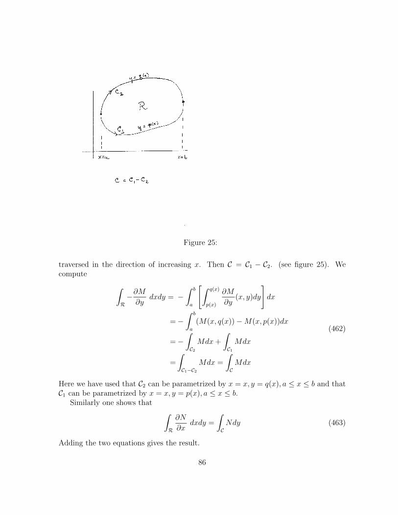
Figure 25:
traversed in the direction of increasing x. Then C = C1 − C2. (see figure 25). Wecompute ∫
R−∂M∂y
dxdy = −∫ b
a
[∫ q(x)
p(x)
∂M
∂y(x, y)dy
]dx
=−∫ b
a
(M(x, q(x))−M(x, p(x))dx
=−∫C2Mdx+
∫C1Mdx
=
∫C1−C2
Mdx =
∫CMdx
(462)
Here we have used that C2 can be parametrized by x = x, y = q(x), a ≤ x ≤ b and thatC1 can be parametrized by x = x, y = p(x), a ≤ x ≤ b.
Similarly one shows that ∫R
∂N
∂xdxdy =
∫CNdy (463)
Adding the two equations gives the result.
86
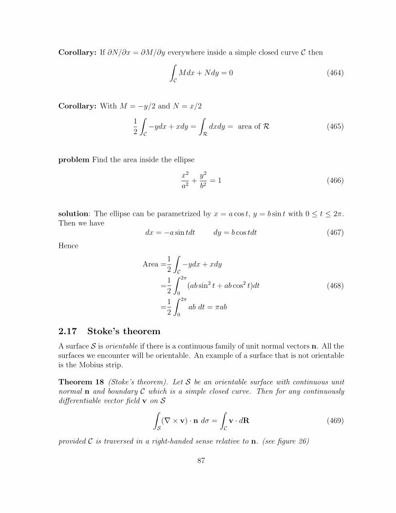
Corollary: If ∂N/∂x = ∂M/∂y everywhere inside a simple closed curve C then∫CMdx+Ndy = 0 (464)
Corollary: With M = −y/2 and N = x/2
1
2
∫C−ydx+ xdy =
∫Rdxdy = area of R (465)
problem Find the area inside the ellipse
x2
a2+y2
b2= 1 (466)
solution: The ellipse can be parametrized by x = a cos t, y = b sin t with 0 ≤ t ≤ 2π.Then we have
dx = −a sin tdt dy = b cos tdt (467)
Hence
Area =1
2
∫C−ydx+ xdy
=1
2
∫ 2π
0
(ab sin2 t+ ab cos2 t)dt
=1
2
∫ 2π
0
ab dt = πab
(468)
2.17 Stoke’s theorem
A surface S is orientable if there is a continuous family of unit normal vectors n. All thesurfaces we encounter will be orientable. An example of a surface that is not orientableis the Mobius strip.
Theorem 18 (Stoke’s theorem). Let S be an orientable surface with continuous unitnormal n and boundary C which is a simple closed curve. Then for any continuouslydifferentiable vector field v on S∫
S(∇× v) · n dσ =
∫Cv · dR (469)
provided C is traversed in a right-handed sense relative to n. (see figure 26)
87

Figure 26:
Proof. We have
(∇× v) · n = det
i j k∂/∂x ∂/∂y ∂/∂zv1 v2 v3
· n
=(∂v3
∂y− ∂v2
∂z
)n1 +
(∂v1
∂z− ∂v3
∂x
)n2 +
(∂v2
∂x− ∂v1
∂y
)n3
(470)
We pick out the the v1 part of this and show∫S
(∂v1
∂zn2 −
∂v1
∂yn3
)dσ =
∫Cv1dx (471)
There will be similar equations for the v2 part and the v3 and when we add themtogether we get the result.
Suppose that S is given as the graph of a function z = φ(x, y) with (x, y) in E andupward normal n. (see figure 27). Then
ndσ = d~σ = (−φxi− φyj + k) dxdy (472)
88
Figure 27:
and so ∫S
(∂v1
∂zn2 −
∂v1
∂yn3
)dσ
=
∫E
(∂v1
∂z(x, y, φ(x, y))(−φy(x, y))− ∂v1
∂y(x, y, φ(x, y)) · 1
)dxdy
=
∫E
− ∂
∂y
[v1(x, y, φ(x, y))
]dxdy
=
∫C′v1(x, y, φ(x, y))dx
=
∫Cv1(x, y, z)dx
(473)
Here C ′ is a boundary curve for E and the second to last step follows by Green’stheorem. The last step follows since if (x, y) traverses C ′ then (x, y, φ(x, y)) traversesC.
example: Let S be the graph of the paraboloid z = 1− x2 − y2 which lies above thedisc x2 + y2 ≤ 1 and let n be the the upward normal. Also let v = yi + zj + xk. Wecheck Stokes theorem in this case.
89
First for the surface integral we have
ndσ = d~σ = (−∂z∂x
i− ∂z
∂yj + k) dxdy = (2xi + 2yj + k)dxdy (474)
Also
∇× v = det
i j k∂/∂x ∂/∂y ∂/∂zy z x
= −i− j− k (475)
Therefore ∫S(∇× v) · d~σ =
∫x2+y2≤1
(−2x− 2y − 1)dxdy
=
∫ 2π
0
∫ 1
0
(−2r cos θ − 2r sin θ − 1) rdrdθ
=2π
∫ 1
0
(−r)dr = −π
(476)
For the line line integral note that C, the boundary of S, is the circle x2 + y2 =1, z = 0. We want to go around it counterclockwise so we parametrize by
R = cos t i + sin t j 0 ≤ t ≤ 2π (477)
Then
dR =(− sin t i + cos t j) dt
v = sin t i + cos t k(478)
and so ∫Cv · dR =
∫ 2π
0
(− sin2 t)dt = −π (479)
as expected.
circulation: Suppose v(R) describes the velocity of a fluid at R, and C is a directedsimple closed curve. We define
circulation of v around C =
∫Cv · dR =
∫C(v ·T)ds (480)
This tells how much the fluid is circulating around the curve. See figure 28.
what is curl? Now we can answer this question, still thinking of v(R) as the velocityof a fluid at R. Given R and a unit vector n, let Sε be the disc centered on R with
90

Figure 28: circulation
radius ε and normal n, and let Cε be the circle which is the boundary of Sε. Then wehave by Stoke’s theorem
(∇× v)(R) · n = limε→0
1
area of Sε
∫Sε
(∇× v) · n dσ
= limε→0
1
area of Sε
∫Cε
v · dR
= circulation density of v around n at R.
(481)
general remark: In thinking about the fundamental theorem of calculus, Green’stheorem, Stoke’s theorem, and the divergence theore note that they all have the form∫
(region)
(derivative of function) =
∫(boundary of region)
(function) (482)
This may help in remembering them. It also suggests that there is a more generaltheorem of this form which holds in any dimension. This is true. It is also calledStoke’s theorem and uses a general theory of differential forms.
91

2.18 still more line integrals
We investigate when line integrals are independent of the path.
Theorem 19 If v = ∇u and C is any curve from R0 to R1 then∫Cv · dR =
∫C∇u · dR = u(R1)− u(R0) (483)
So in this case the integral is independent of the path taken from R0 to R1. Wecan write without ambiguity. ∫ R1
R0
v · dR (484)
Another way to write this is to define the differential du by
du =∂u
∂xdx+
∂u
∂ydy +
∂u
∂zdz = ∇u · dR (485)
Then the theorem says that for any path C from R0 to R1∫Cdu = u(R1)− u(R0) (486)
Proof. Suppose C is parametrized by R(t) with a ≤ t ≤ b. Then R(a) = R0 andR(b) = R1 and we have by the chain rule∫
C∇u · dR =
∫ b
a
∇u(R(t)) · dRdt
dt
=
∫ b
a
d
dt
(u(R(t))
)dt
=u(R(b))− u(R(a))
=u(R1)− u(R0)
(487)
application: Suppose F(R) is the force applied to an object at R. As noted before∫C F · dR is the work done in moving the object along C. If C goes from R0 to R1 and
F = ∇u then the work is u(R1) − u(R0) independent of C. In this case one says thatthe force is conservative and u is called the potential energy .
For example the electrostatic force around a charge at the origin has the form
F(R) = −C R
|R|3(488)
92

This is a conservative force with potential (check it)
u(R) =C
|R|(489)
definition: A region R in R3 is connected if any two points in R can be joined bya continuous curve in R.
Theorem 20 Let v be a vector field in a connected region R in R3. Then the followingstatements are equivalent (i.e. either they are all true or all false)
1.∫C v · dR = 0 for any closed curve C in R.
2.∫C v · dR = 0 is independent of the path C in R (C with fixed endpoints in R).
3. v = ∇u for some function u in R.
Proof. First we show that (1.) implies (2.). If (1.) is true and C1 and C2 are any twopaths from R0 to R1 then C1 − C2 is a closed curve and so∫
C1v · dR−
∫C2
v · dR =
∫C1−C2
v · dR = 0 (490)
Thus (2.) is true.By a similar argument one can show that (2.) implies (1.). Thus (1.) and (2.) are
equivalent.We already know that (3.) implies (2.). Thus we need only show that (2.) implies
(3.). Assuming (2.) we define for any point R0 in R
u(R) =
∫ R
R0
v(R′) · dR′ (491)
Because R is connected there are paths from R0 to R and because integrals are inde-pendent of path we do not have to specifiy which one.
93

We have to show that the gradient of u is v. We compute
∂u
∂x(R) = lim
h→0
1
h(u(R + hi)− u(R))
= limh→0
1
h
[ ∫ R+hi
R0
v(R′) · dR′ −∫ R
R0
v(R′) · dR′]
= limh→0
1
h
[ ∫ R+hi
R0
v(R′) · dR′ +∫ R0
R
v(R′) · dR′]
= limh→0
1
h
[ ∫ R+hi
R
v(R′) · dR′]
= limh→0
1
h
[ ∫ h
0
v1(R + ti)dt]
=v1(R)
(492)
Here in the second to last step we have chosen a particular path from R to R + hi,namely R′ = R + ti with 0 ≤ t ≤ h and dR′ = idt.
Similarly one shows that (∂u/∂y)(R) = v2(R) and (∂u/∂z)(R) = v3(R) and hence∇u(R) = v(R). This completes the proof.
example: Consider again the vector field
v = yz2i + xz2j + (2xyz + z)k (493)
Are integrals∫C v · dR independent of path in R3? According to the theorem this is
the same as asking whether v = ∇u. If there is such a u it must satisfy
∂u
∂x=yz2
∂u
∂y=xz2
∂u
∂z=2xyz + z
(494)
The first equation says that u = xyz2 + h(y, z) for some function h. Taking derivativesof this we have
∂u
∂y=xz2 +
∂h
∂y∂u
∂z=2xyz +
∂h
∂z
(495)
Comparing this with the second and third equations above yields
∂h
∂y= 0
∂h
∂z= z (496)
94

The second equation says h(y, z) = 12z2 + g(y) for some function g. But then the first
equation implies that g(y) = C for some constant C. Thus h(y, z) = 12z2 + C for some
constant C. Therefore
u = xyz2 +1
2z2 + C (497)
is the function we are looking for and the answer is yes.
The theorem actually holds in any dimension. We state the theorem for R2 in thelanguage of differential forms.
Theorem 21 Let M,N be functions in a connected region R in R2. Then the followingstatements are equivalent
1.∫CMdx+Ndy = 0 for any closed curve C in R.
2.∫CMdx+Ndy = 0 is independent of the path C in R.
3. M = ∂u/∂x and N = ∂u/∂y for some function u in R, i.e. Mdx+Ndy = du.
definition: A region R is simply connected if it is connected and every simple closedcurve can be continuously shrunk to a point without leaving R. Figure 29 gives someexamples.
Theorem 22 If v is a continuously differentiable vector field in a simply connectedregion R then the conditions (1.), (2.), (3.) of the last two theorems are equivalent to
(4.)
{∇× v = 0 in R ⊂ R3
∂N/∂x− ∂M/∂y = 0 in R ⊂ R2(498)
Proof. We give the proof for R3. (3.) says that v = ∇u and we know that this implies∇× v = 0 which is (4.).
On the other hand suppose that (4.) is true. Since R is simply connected everysimple closed curve C in R is the boundary of a surface S in R - the curves shrinkingdown C sweep out the surface. Then by Stokes theorem∫
Cv · dR =
∫S(∇× v) · n dσ = 0 (499)
Thus (1.) is true for simple closed curves. But closed curve that is not simple can bebroken up into pieces that are simple. Thus (1.) is true in general.
95
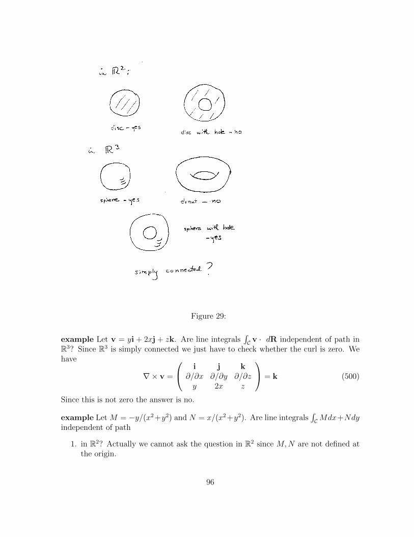
Figure 29:
example Let v = yi + 2xj + zk. Are line integrals∫C v · dR independent of path in
R3? Since R3 is simply connected we just have to check whether the curl is zero. Wehave
∇× v =
i j k∂/∂x ∂/∂y ∂/∂zy 2x z
= k (500)
Since this is not zero the answer is no.
example Let M = −y/(x2 +y2) and N = x/(x2 +y2). Are line integrals∫CMdx+Ndy
independent of path
1. in R2? Actually we cannot ask the question in R2 since M,N are not defined atthe origin.
96

2. in R2 with the origin deleted? This is not simply connected so we cannot use thetest ∂N/∂x− ∂M/∂y = 0. No conclusion.
3. in R2 with the negative x-axis deleted? This is simply connected so we can applythe test and if we do we find that ∂N/∂x− ∂M/∂y = 0 (check it). So the answeris yes.
We can say more. Since we do have path independence there must be a u so thatM = ∂u/∂x and N = ∂u/∂y. By solving these equations one finds
u(x, y) = tan−1(yx
)= polar angle of (x, y) (501)
This works in the region (3.), but not in the region (2.) since the function is notcontinuous across the negative x-axis. It takes the value π from above and −π frombelow. In fact there is no function in the entire region (2.) and the answer to thequestion is no.
definitions A vector field v is irrotational if ∇×v = 0. We have seen that in a simplyconnected region this occurs if and only if v = ∇u for some scalar u. A vector field issolenoidal is ∇ · v = 0. One can show that in a simply connected region this occurs ifand only if v = ∇×w for some vector field w.
It is a theorem that in a simply connected region every vector field v can be writtenin the form v = v1 + v2 where v1 is solenoidal and v2 is irrotational.
2.19 more applications
We discuss some applications to electromagnetism. The players in our drama are anelectric field E(R, t), a magnetic field B(R, t), a current density j(R, t) and a chargedensity ρ(R, t). These are time dependent vector fields, except the charge density whichis a time dependent scalar.
The charge density and the current obey the charge conservation equation
∇ · j +dρ
dt= 0 (502)
This can be derived just as we derived the continuity equation for fluid flow. The fieldsobey Maxwell’s equations:
∇ · E =4πρ
∇ ·B =0
∇× E =− 1
c
∂B
∂t
∇×B =1
c
∂E
∂t+
4π
cj
(503)
97
Here c is a constant of nature (3× 1010cm/sec).
We work out some special cases, assuming we are in a simply connected region.
1. Suppose B is constant in the time t. Then third equation says that ∇× E = 0.This means that E is the gradient of a scalar. We write
E = −∇Φ (504)
and Φ is called the electromagnetic potential. Inserting this equation into thefirst gives
−∆Φ = 4πρ (505)
This known as Poisson’s equation. It is easier to solve than the full Maxwellsystem and a great deal of mathematics is devoted to its solution. Especiallyimportant is the case ρ = 0 in which case we again have Laplace’s equation:
∆Φ = 0 (506)
2. The second equation ∇ ·B = 0 implies that
B = ∇×A (507)
for some vector field A known as the magnetic potential. The potential can bewritten A = A1 + A2 where ∇ · A1 = 0 and ∇ × A2 = 0. However A2 doesnot contribute to B so we can take A = A1 and still have B = ∇ ×A . Then∇ ·A = ∇ ·A1 = 0.
If E is constant in time, then the last Maxwell equation becomes
∇× (∇×A) =4π
cj (508)
But by one of our vector identities
∇× (∇×A) = ∇(∇ ·A)−∆A = −∆A (509)
thus our equation becomes
−∆A =4π
cj (510)
Thus each component of A satisfies Poisson’s equation and so is amenable tosolution.
3. Now suppose both ρ and j are zero. Then the equations become
∇ · E =0
∇ ·B =0
∇× E =− 1
c
∂B
∂t
∇×B =1
c
∂E
∂t
(511)
98

Taking the curl of the last equation, and using the third yields
∇× (∇×B) =1
c
∂
∂t(∇× E) = − 1
c2
∂2B
∂t2(512)
But on the other hand
∇× (∇×B) = ∇(∇ ·B)−∆B = −∆B (513)
Comparing the last two gives
1
c2
∂2B
∂t2−∆B = 0 (514)
This is called the wave equation and has also been studied at length. By a similarargument we can also show the E obeys the same equation:
1
c2
∂2E
∂t2−∆E = 0 (515)
A characteristic feature of solutions of these equations is that disturbances propa-gate with speed c. But c is the speed of light. This makes it possible to interpretlight as waves in the electromagnetic field. This was one of the triumphs ofMaxwell’s equations.
2.20 general coordinate systems
Consider a differentiable invertible function
x =x(u1, u2, u3)
y =y(u1, u2, u3)
z =z(u1, u2, u3)
(516)
from some region R′ ⊂ R3 onto R ⊂ R3. Then u = (u1, u2, u3) in R′ can be consideredas new coordinates for R. These were considered previously in our change of variablesformula for R3. In a vector notation we have
R(u) = x(u1, u2, u3)i + y(u1, u2, u3)j + z(u1, u2, u3)k (517)
As before we let ∂R/∂ui be the tangent vector to a ui-line. The length of thesevectors are called the scale factors :
hi = hi(u) = |∂R/∂ui| (518)
We also consider
ei = ei(u) =1
hi
∂R
∂ui(519)
99

which are unit tangent vectors to the ui-lines.Our assumption of invertibility implies that
∂(x, y, z)
∂(u1, u2, u3)6= 0 (520)
(This is a converse to the inverse function theorem). This is a determinant with columns∂R/∂ui. It follows that ∂R/∂u1, ∂R/∂u2, ∂R/∂u3 are linearly independent. Hencee1, e2, e3 are linearly independent and so form a basis for R3. Any vector v in R3 canbe uniquely written in the form
v = v1e1 + v2e2 + v3e3 =3∑i=1
viei (521)
The new coordinates are said to be orthogonal if
∂R
∂ui· ∂R
∂uj= 0 for i 6= j (522)
It is equivalent to say that
ei · ej =
{0 i 6= j
1 i = j(523)
and the ei form an orthonormal basis. Then v · ei = vi and we can write
v =3∑i=1
(v · ei)ei (524)
For the rest of this section we assume we have an orthogonal coordinate system.We give some examples of orthogonal coordinate systems.
1. (cylindrical coordinates) These are defined by
R = r cos θi + r sin θj + zk (525)
We computed ∂R/∂r, ∂R/∂θ, ∂R/∂z, saw that they were orthogonal, and com-puted er, eθ, ez. The scale factors are
hr =|∂R/∂r| = 1
hθ =|∂R/∂θ| = r
hz = |∂R/∂z| = 1
(526)
100
2. (spherical coordinates) These are defined by
R = ρ sinφ cos θi + ρ sinφ sin θj + ρ cosφk (527)
We computed ∂R/∂ρ, ∂R/∂φ, ∂R/∂θ. One can check that they are orthogonal.Also we computed eρ, eφ, eθ. The scale factors are
hρ =|∂R/∂ρ| = 1
hφ =|∂R/∂φ| = ρ
hθ =|∂R/∂θ| = ρ sinφ
(528)
3. (parbolic coordinates) These are defined by
R = (u1u2 cosu3)i + (u1u2 sinu3)j +1
2(u2
1 − u22)k (529)
We compute
∂R/∂u1 =u2 cosu3i + u2 sinu3j + u1k
∂R/∂u2 =u1 cosu3i + u1 sinu3j− u2k
∂R/∂u3 =u1u2(− sinu3)i + u1u2(cosu3)j
(530)
These are orthogonal since for example
∂R
∂u1
· ∂R
∂u2
= u1u2 cos2 u3 + u1u2 sin2 u3 − u1u2 = 0 (531)
The other pairs are similar. The scale factors are
h1 =|∂R/∂u1| =√u2
1 + u22
h2 =|∂R/∂u2| =√u2
1 + u22
h3 =|∂R/∂u3| = u1u2
(532)
From the above one can compute e1, e2, e3.
Orthogonal coordinate systems are special; there are only a finite number of them.A vector field v(R) in new coordinates R(u) is
v(u) = v(R(u)) (533)
The vector field in new coordinates and new basis ei(u) is
v(u) =3∑i=1
vi(u)ei(u) vi(u) = v(u) · ei(u) (534)
101
example: Consider the vector field
v = yi + xj + zk (535)
In cylindrical coordinates this is
v = r sin θi + r cos θj + zk (536)
We want to express it in the cylindrical basis
er = cos θi + sin θj
eθ =− sin θi + cos θj
ez =k
(537)
It will have the formv = vrer + vθeθ + vzez (538)
where
vr =v · er = 2r cos θ sin θ = r sin(2θ)
vθ =v · eθ = −r sin2 θ + r cos2 θ = r cos(2θ)
vz =v · ez = z
(539)
Thusv = r sin(2θ)er + r cos(2θ)eθ + zez (540)
Now suppose we are given a scalar function f(R) and a vector field v(R). Weconsider the problem of expressing the derivatives ∇f,∇ · v,∇ × v,∆f in a generalorthogonal coordinate system R = R(u) with orthonormal basis ei(u).
We start with the gradient. In new coordinates f(u) = f(R(u)) The new gradientis defined as
( grad f)(u) ≡ (∇f)(R(u)) =3∑i=1
[(∇f)(R(u)) · ei(u)]· ei(u) (541)
But the derivatives are still in Cartesian coordinates. By the chain rule
∂f
∂ui(u) = (∇f)(R(u)) · ∂R
∂ui= (∇f)(R(u)) · ei(u)hi(u) (542)
Therefore
(∇f)(R(u)) · ei(u) =1
hi(u)
∂f
∂ui(u) (543)
102

Substituting this into the expression for grad f we find that
( grad f)(u) =3∑i=1
1
hi(u)
∂f
∂ui(u)ei(u) (544)
examples: In cylindrical coordinates
grad f =1
hr
∂f
∂rer +
1
hθ
∂f
∂θeθ +
1
hz
∂f
∂zez
=∂f
∂rer +
1
r
∂f
∂θeθ +
∂f
∂zez
(545)
In spherical coordinates
grad f =1
hρ
∂f
∂ρeρ +
1
hφ
∂f
∂φeφ +
1
hθ
∂f
∂θeθ
=∂f
∂ρeρ +
1
ρ
∂f
∂φeφ +
1
ρ sinφ
∂f
∂θeθ
(546)
example . Consider the function
f(R) =1
|R|=
1√x2 + y2 + z2
(547)
We want to find the gradient. It is easiest to change to spherical coordinates by
f(ρ, φ, θ) =1
ρ(548)
Then since this function does not depend on φ or θ
grad f =∂f
∂ρeρ = − 1
ρ2eρ (549)
(And since ρ = |R| and eρ = R/|R| this is −R/|R|3 back in Cartesian coordinates.)
Next consider the divergence. Recall that a vector field v(R) is expressed in newcoordinates R(u) by v(u) = v(R(u)) and that in the new basis it has the form v =∑
i viei with vi = v · ei. The divergence of the vector field is defined by ( div v)(u) =(∇ · v)(R(u)). Then one can show that (after a somewhat lengthy calculation)
div v =1
h1h2h3
(∂(h2h3v1)
∂u1
+∂(h1h3v2)
∂u2
+∂(h1h2v3)
∂u3
)(550)
103

For example consider spherical coordinates with hρ = 1, hφ = ρ, hθ = ρ sinφ. Thenwe have
v = vρeρ + vφeφ + vθeθ (551)
and
div v =1
ρ2 sinφ
(∂(ρ2 sinφvρ)
∂ρ+∂(ρ sinφvφ)
∂φ+∂(ρvθ)
∂θ
)=
1
ρ2
∂(ρ2vρ)
∂ρ+
1
ρ sinφ
(∂(sinφvφ)
∂φ+∂vθ∂θ
) (552)
For a general coordinate system the curl is ( curl v)(u) = (∇× v)(R(u)). One canshow that
curl v =1
h1h2h3
det
h1e1 h2e2 h2e3
∂/∂u1 ∂/∂u2 ∂/∂u3
h1v1 h2v2 h3v3
(553)
Finally for a scalar if f(u) = f(R(u)) and (∆f)(u) = (∆f)(R(u)) then one canshow
∆f =1
h1h2h3
(∂
∂u1
(h2h3
h1
∂f
∂u1
)+
∂
∂u2
(h1h3
h2
∂f
∂u2
)+
∂
∂u3
(h1h2
h3
∂f
∂u3
))(554)
For example in spherical coordinates
∆f =1
ρ2 sinφ
(∂
∂ρ
(ρ2 sinφ
∂f
∂ρ
)+
∂
∂φ
(sinφ
∂f
∂φ
)+
∂
∂θ
(1
sinφ
∂f
∂θ
))
=1
ρ2
∂
∂ρ
(ρ2∂f
∂ρ
)+
1
ρ2 sinφ
∂
∂φ
(sinφ
∂f
∂φ
)+
1
ρ2 sin2 φ
∂2f
∂θ2
(555)
example Find all spherically symmetric solutions of ∆f = 0. Spherically symmet-ric means that f(R) depends only on |R|. In spherical coordinates it means thatf(ρ, φ, θ) = f(ρ). Then the equation is
∆f =1
ρ2
∂
∂ρ
(ρ2∂f
∂ρ
)= 0 (556)
This implies
ρ2∂f
∂ρ= c1 (557)
for some constant c1. Then∂f
∂ρ=c1
ρ2(558)
104

which has the general solution
f(ρ) =−c1
ρ+ c2 (559)
Back in Cartesian coordinates it says that
f(R) =−c1
|R|+ c2 (560)
105
3 complex variables
3.1 complex numbers
A complex number is a pair of real numbers, hence a vector in R2. It is written
z = (x, y) (561)
Define addition and multiplication by a scalar just as for vectors:
z1 + z2 =(x1 + x2, y1 + y2)
αz =(αx, αy) α ∈ R(562)
We also define multiplication by
z1z2 = (x1x2 − y1y2, x1y2 + y1x2) (563)
Then, as one can check, the ordinary rules of arithmetic apply:
z1(z2z3) =(z1z2)z3
z1z2 =z2z1
z1(z2 + z3) =z1z2 + z1z3
(564)
Two special complex numbers are
1 = (1, 0) i = (0, 1) (565)
Then any complex z can be written
z = (x, y) = x(1, 0) + y(0, 1) = x1 + yi (566)
Consider complex numbers of the form x1. We have
(x11)(x21) =(x1, 0)(x2, 0) = (x1x2, 0) = x1x21
x11 + x21 =(x1, 0) + (x2, 0) = (x1 + x2, 0) = (x1 + x2)1
(x1)(x′, y′) =(x, 0)(x′, y′) = (xx′, xy′) = x(x′, y′)
(567)
These behave just like the real numbers. Hence we can identify the complex numberx1 = (x, 0) with the real number x
Now consider complex numbers of the from yi. We have
(y1i)(y2i) = (0, y1)(0, y2) = (−y1y2, 0) = −y1y21 = −y1y2 (568)
In particular(yi)2 = −y2 i2 = −1 (569)
106
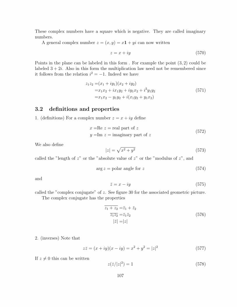
These complex numbers have a square which is negative. They are called imaginarynumbers.
A general complex number z = (x, y) = x1 + yi can now written
z = x+ iy (570)
Points in the plane can be labeled in this form . For example the point (3, 2) could belabeled 3 + 2i. Also in this form the multiplication law need not be remembered sinceit follows from the relation i2 = −1. Indeed we have
z1z2 =(x1 + iy1)(x2 + iy2)
=x1x2 + ix1y2 + iy1x2 + i2y1y2
=x1x2 − y1y2 + i(x1y2 + y1x2)
(571)
3.2 definitions and properties
1. (definitions) For a complex number z = x+ iy define
x =Re z = real part of z
y =Im z = imaginary part of z(572)
We also define|z| =
√x2 + y2 (573)
called the ”length of z” or the ”absolute value of z” or the ”modulus of z”, and
arg z = polar angle for z (574)
andz = x− iy (575)
called the ”complex conjugate” of z. See figure 30 for the associated geometric picture.The complex conjugate has the properties
z1 + z2 =z1 + z2
z1z2 =z1z2
|z| =|z|(576)
2. (inverses) Note that
zz = (x+ iy)(x− iy) = x2 + y2 = |z|2 (577)
If z 6= 0 this can be writtenz(z/|z|2) = 1 (578)
107
Figure 30:
This says that z/|z|2 is an inverse for z. We write
z−1 =z
|z|2or (x+ iy)−1 =
x− iyx2 + y2
(579)
Then we can divide by any z 6= 0 by defining
w
z= wz−1 (580)
examples: By the formula i−1 = −i and
(3 + 4i)−1 =3− 4i
25=
3
25− i 4
25(581)
However one does not have to remember the formula. Instead just multiply in thenumerator and denominator by the complex conjugate. For example
1
3 + 4i=
1
3 + 4i· 3− 4i
3− 4i=
3− 4i
25
3. (distances) Just as for vectors
|z1 − z2| = distance from z1 to z2 (582)
108

The triangle inequality holds:
||z1| − |z2|| ≤ |z1 ± z2| ≤ |z1|+ |z2| (582)
4. (exponentials) We want to define
ez = ex+iy = exeiy (582)
We know what ex means and we know that it can be expressed as a convergent series
ex = 1 + x+1
2!x2 +
1
3!x3 + . . . (582)
Suppose we try to define eiy in the same way ignoring questions of convergence. Wewould have
eiy =1 + iy +1
2!(iy)2 +
1
3!(iy)3 + . . .
=
(1− 1
2!y2 +
1
4!y4 + . . .
)+ i
(y − 1
3!y3 +
1
5!y5 + . . .
)= cos y + i sin y
(582)
We take this as the definition, that is eiy ≡ cos y + i sin y and more generally
ez = ex+iy = ex(cos y + i sin y) (582)
This does obey the law of exponents:
eiy1eiy2 =(cos y1 + i sin y1)(cos y2 + i sin y2)
=(cos y1 cos y2 − sin y1 sin y2) + i(cos y1 sin y2 + sin y1 cos y2)
= cos(y1 + y2) + i sin(y1 + y2)
=ei(y1+y2)
(582)
and in general ez1ez2 = ez1+z2 . Also note
eiy =cos y + i sin y = cos y − i sin y = cos(−y) + i sin(−y) = e−iy
|eiy| = cos2 y + sin2 y = 1
(eiy)−1 =eiy
|eiy|2= e−iy
(582)
The last could also be deduced from the law of exponents.
examples:
ei0 = 1 eiπ/2 = i eiπ = −1 ei3π/2 = −i ei2π = 1 (582)
e3+iπ/4 = e3(cosπ/4 + i sinπ/4) = e3
(1√2
+ i1√2
)(582)
109
3.3 polar form
Points in the plane have polar coordinates (r, θ) related to Cartesian coordinate byx = r cos θ, y = r sin θ. A complex number can then be written in polar form by
z = x+ iy = r cos θ + ir sin θ = reiθ (582)
Every point z 6= 0 has a unique polar representation z = reiθ with r > 0 and 0 ≤ θ < 2π.Now we have
|z| = r arg z = θ (582)
If z1 = r1eiθ1 and z2 = r2e
iθ2 then the product is
z1z2 = r1r2ei(θ1+θ2) (582)
This says that in complex multiplication we multiply lengths and add angles. Anotherway to write it is
|z1z2| =|z1||z2|arg(z1z2) = arg(z1) + arg(z2)
(582)
The second equation only holds if both sides are in the interval [0, 2π). For example ifz1 = z2 = −i, then arg(z1) + arg(z2) = 3π/2 + 3π/2 = 3π but arg(z1z2) = arg(−1) = πand the identity fails.
examples
1. To find the polar form of z = 1 + i√
3 note that the length is 2 and the angle istan−1(
√3) = π/3 hence z = 2eiπ/3.
2. To find the polar form of z = 1 + i note that the length is√
2 and the angle istan−1(1) = π/4. Thus z =
√2eiπ/4.
3. To find (1 + i)8 write it in polar form and compute
(1 + i)8 = (√
2eiπ/4)8 = 24e2πi = 16 (582)
problem: Find all complex z such that z3 = 1
solution: Try z = reiθ with r > 0 and 0 ≤ θ < 2π. This is a solution if
r3ei3θ = 1 (582)
Comparing lengths gives r3 = 1 and so r = 1. Then θ must satisfy ei3θ = 1 orcos(3θ) = 1, sin(3θ) = 0. The solutions are
3θ = 0,±2π,±4π,±6π, . . . (582)
110

orθ = 0,±2π/3,±4π/3,±6π/3, . . . (582)
But the only solutions with 0 ≤ θ < 2π are θ = 0, 2π/3, 4π/3. Thus the answer is
z = ei0, ei2π/3, ei4π/3 = 1, −1
2+
√3
2i, −1
2−√
3
2i (582)
One of the uses of complex numbers is that every polynomial has complex roots. Inthe problem we found the solutions of z3 − 1 = 0. Here are some more examples:
examples:
1. The equation zn = a (a real) has n solutions:
z = a1/n, a1/nei(2π/n), a1/nei2(2π/n), . . . , a1/nei(n−1)(2π/n) (582)
2. The equation az2 + bz + c = 0 (a, b, c real) has solutions
z =
−b±√b2−4ac
2aif b2 − 4ac > 0
−b2a
if b2 − 4ac = 0−b±i
√4ac−b2
2aif b2 − 4ac < 0
(582)
3.4 functions
Let C stand for the set of all complex numbers. Thus C is R2 with a special multipli-cation. We are interested in functions from C (or a subset) to C written w = f(z) withboth w, z complex. For example w = z2 or w = 1/(3z + 2) or w = |z|.
If w = u+ iv and
f(z) = f(x+ iy) = u(x, y) + iv(x, y) (582)
then the equation w = f(z) can be written as the pair of equations
u = u(x, y) v = v(x, y) (582)
The function u(x, y) is called the real part and the function v(x, y) is called the imagi-nary part.
examples
1. If w = ez = ex(cos y + i sin y) then
u = ex cos y v = ex sin y (582)
111

Figure 31: mapping by the function w = z2
2. If w = 1/z = (x− iy)/(x2 + y2) then
u =x
x2 + y2v =
−yx2 + y2
(582)
To represent a function w = f(z) geometrically we show how it affects straight lines.
example: Consider the function w = z2 which takes the first quadrant to the upperhalf plane. We have w = z2 = (x + iy)2 = (x2 − y2) + i2xy so it is equivalent to thepair of functions
u = x2 − y2 v = 2xy (582)
It maps the line x = c, y > 0 to the line u = c2 − y2, v = 2cy which is the halfparabola
u = c2 − v2
4c2, v > 0 (582)
It maps the line y = c, x > 0 to the line u = x2− c2, v = 2xc which is the half parabola
u =v2
4c2− c2, v > 0 (582)
This is represented in figure 31.
112

3.5 special functions
(A.) trigonometric functionsIf y is real so eiy = cos y + i sin y and e−iy = cos y − i sin y then
1
2(eiy + e−iy) = cos y
1
2(eiy − e−iy) = i sin y (582)
Accordingly we define for complex z
cos z =1
2(eiz + e−iz) sin z =
1
2i(eiz − e−iz) (582)
Other trig functions can be defined from these, for example
tan z =sin z
cos z(582)
If z = iα is purely imaginary then
cos(iα) =1
2(e−α + eα) = coshα
sin(iα) =1
2i(e−α − eα) = i
1
2(eα − e−α) = i sinhα
(582)
Thus the complex trig functions include both the usual trig functions and the hyperbolictrig functions as special cases.
(B.) logarithmWe want to define the natural logarithm log z of a complex number z. If z 6= 0 and
such a log has the same properties as the log of positive numbers then we expect
log z = log reiθ = log r + log eiθ = log r + iθ (582)
Accordingly we take as the definition for z 6= 0
log z = log |z|+ i arg z (582)
where 0 ≤ arg z < 2π. However sometimes we may want to make another choice of thepolar angle arg z. For example we could take −π ≤ arg z < π or more generally
c ≤ arg z < c+ 2π (582)
Each choice of c gives a different log functions, called a branch of the logarithm. Analternative is to take all possible values of arg z. If θ is one possible value then thesewould be the infinite sequence
. . . , θ − 2π, θ, θ + 2π, θ + 4π, . . . (582)
113

In this case we have a multi-valued function.
example: Take the branch of log z with 0 ≤ arg z < 2π. Then
log i = log |i|+ i arg i = iπ
2log(−2) = log | − 2|+ i arg(−2) = log 2 + iπ
log(−3i) = log | − 3i|+ i arg(−3i) = log 3 + i3π
2
log(1 + i) = log |1 + i|+ i arg(1 + i) = log√
2 + iπ
4
(582)
Is the logarithm the inverse of the exponential? We have the following result
Theorem 23
1. For any branch of the logarithm
elog z = z (582)
2. If log z is defined with c ≤ arg z < c + 2π and if z = x + iy with c ≤ y < c + 2πthen
log(ez) = z (582)
Proof. For the first if z = reiθ, then log z = log r + i(θ + 2πk) for some k. Then
elog z = elog reiθei2πk = reiθ = z (582)
For the second since the restriction on y matches the definition of arg
log(ez) = log(exeiy) = log ex + i arg eiy = x+ iy = z (582)
(C.) complex exponentialsSince z = elog z we can define for complex z, w
zw = ew log z (582)
Here we have to specify the branch of the logarithm we are using. An alternative is totake all possible values of log z and get a multi-valued function zw.
If w is a positive integer n then
zn (new) = en log z = (elog z)n = zn (old) (582)
114

is the same for any branch of the logarithm. But
z1/n = elog z/n (582)
will have n different values depending on the branch of the log. Each value does satisfy(z1/n)n = elog z = z.
example Since log 1 = i arg 1
11/3 = e13
log 1 = ei3
arg 1 =
1 if arg 1 = 0
ei2π/3 if arg 1 = 2π
ei4π/3 if arg 1 = 4π
(582)
We find the solutions of z3 = 1 as z = 11/3 with the different branches for the cuberoot.
example Since log i = i arg i
i1/3 = e13
log i = ei3
arg i =
eiπ/6 if arg i = π
2
ei5π/6 if arg i = 5π2
ei9π/6 if arg i = 9π2
(582)
example Since log i = i arg iii = ei log i = e− arg i (582)
This takes infinitely many values
. . . , e3π/2, e−π/2, e−5π/2, e−9π/2, . . . (582)
3.6 derivatives
(A.) First consider functions from R to C written z = f(t) where z is complex and t isreal. For example z = eit or z = t2 + i log t. Such a function can always be written
z = f(t) = x(t) + iy(t) (582)
and x(t) is called the real part of the function and y(t) is called the imaginary part ofthe function. The derivative is defined just as for a vector valued function:
dz
dt= f ′(t) = x′(t) + iy′(t) (582)
115

example: Ifz = eiat = cos(at) + i sin(at) a real (582)
thendz
dt= −a sin(at) + ia cos(at) = ia(cos(at) + i sin(at)) = iaeiat (582)
(B.) Now consider functions from C to C written w = f(z). We start with the definitionof a limit.
definition: limz→z0 f(z) = w0 means for every ε > 0 there is a δ > 0 so if |z − z0| < δthen |f(z)− w0| < ε.
This says that f(z)→ w0 as z → z0 from any direction.Now write
z = x+ iy z0 = x0 + iy0
f(z) = u(x, y) + iv(x, y) w0 = u0 + iv0
(582)
Then
|f(z)− w0| =√
(u(x, y)− u0)2 + (v(x, y)− v0)2
|z − z0| =√
(x− x0)2 + (y − y0)2(582)
From this we deduce that limz→z0 f(z) = w0 is the same as
lim(x,y)→(x0,y0)
u(x, y) = u0
lim(x,y)→(x0,y0)
v(x, y) = v0
(582)
definition: w = f(z) is continuous at z0 if limz→z0 f(z) = f(z0)
This is the same as the statement that u(x, y) and v(x, y) are continuous at (x0, y0).One can show that if f, g are continuous at z0 then so are f ± g, f · g, and f/g, the lastprovided g(z0) 6= 0. Also if g is continuous at z0 and f is continuous at g(z0) then thecomposition f ◦ g is continuous at z0.
definition: w = f(z) is differentiable at z0 if the derivative
f ′(z0) = lim∆z→0
f(z0 + ∆z)− f(z0)
∆zexists (582)
Varying z0 it is also a function. We also write
dw
dz= f ′(z) (582)
116
Theorem 24 If f is differentiable at z0, then it is continuous at z0
Proof.
limz→z0
f(z)− f(z0) = limz→z0
(f(z)− f(z0)
z − z0
)(z − z0) = f ′(z0) · 0 = 0 (582)
Theorem 25 If f, g are differentiable at z so are f ± g, f · g, f/g (provided g(z) 6= 0)and
(f ± g)′(z) =f ′(z)± g′(z)
(f · g)′(z) =f ′(z)g(z) + f(z)g′(z)(f
g
)′(z) =
g(z)f ′(z)− f(z)g′(z)
g(z)2
(582)
If g is differentiable at z and f is differentiable at g(z) then f ◦ g is differentiable at zand
(f ◦ g)′(z) = f ′(g(z))g′(z) (582)
These are proved just as for real variables.
examples:
1. If f(z) = c then f ′(z) = 0.
2. If f(z) = z then
f ′(z) = lim∆z→0
(z + ∆z)− z∆z
= lim∆z→0
1 = 1 (582)
3. If f(z) = z2 then by the product rule
f ′(z) =dz
dzz + z
dz
dz= 2z (582)
4. If f(z) = zn then f ′(z) = nzn−1.
5. Any polynomial P (z) is differentiable.
6. Any rational function P (z)/Q(z) is differentiable except at points whereQ(z) = 0.(where it is not even defined)
117

example Let f(z) = z. If it exists the derivative is
lim∆z→0
f(z + ∆z)− f(z)
∆z= lim
∆z→0
∆z
∆z(582)
The limit must be the same from any direction. But if ∆z = ∆x is real then
lim∆z→0
∆z
∆z= lim
∆x→0
∆x
∆x= 1 (582)
and ∆z = i∆y is imaginary then
lim∆z→0
∆z
∆z= lim
∆y→0
−i∆yi∆y
= −1 (582)
The limit depends on the direction which means there is no limit in the complex sense.Thus the derivative does not exist. (Even though there are no kinks or discontinuitiesin this function).
3.7 Cauchy-Riemann equations
Let f(z) be differentiable so lim∆z→0(f(z+ ∆z)− f(z))/∆z exists. What does this sayabout the real and imaginary parts f(z) = u(x, y) + iv(x, y)? First let ∆z = ∆x bereal. Then
f ′(z) = lim∆x→0
f(z + ∆x)− f(z)
∆x
= lim∆x→0
(u(x+ ∆x, y)− u(x, y)
∆x
)+ i lim
∆x→0
(v(x+ ∆x, y)v(x, y)
∆x
)=∂u
∂x+ i
∂v
∂x
(583)
Now let ∆z = i∆y be imaginary. Then
f ′(z) = lim∆y→0
f(z + i∆y)− f(z)
i∆y
=1
ilim
∆y→0
(u(x, y + ∆y)− u(x, y)
∆y
)+ lim
∆y→0
(v(x, y + ∆y)− v(x, y)
∆y
)=− i∂u
∂y+∂v
∂y
(584)
These two expressions must agree since the limit must be the same from any direction.Thus we must have
∂u
∂x=∂v
∂y
∂u
∂y= −∂v
∂x(585)
These are the Cauchy-Riemann equations or CR equations.Thus if f(z) is differentiable the the real and imaginary parts satisfy the CR equa-
tions. The converse is also true if we strengthen the hypotheses a bit.
118
Theorem 26 If u(x, y), v(x, y) have continuous partial derivatives which satisfy theCR equations near a point, then f(z) = u(x, y) + iv(x, y) is differentiable at that pointand
f ′(z) =∂u
∂x+ i
∂v
∂x=∂v
∂y− i∂u
∂y(586)
examples
1. Let f(z) = z2 so that u = x2 − y2 and v = 2xy. We have
∂u
∂x= 2x =
∂v
∂y
∂u
∂y= −2y = −∂v
∂x(587)
Thus the CR equations hold so f(z) is differentiable (which we already knew)and
d(z2)
dz=∂u
∂x+ i
∂v
∂x= 2x+ i2y = 2z (588)
(which we also knew)
2. Let f(z) = ez = ex cos y + iex sin y so u = ex cos y, v = ex sin y. Then
∂u
∂x= ex cos y =
∂v
∂y
∂u
∂y= −ex sin y = −∂v
∂x(589)
Thus the CR equations hold so f(z) is differentiable and
d(ez)
dz=∂u
∂x+ i
∂v
∂x= ex cos y + iex sin y = ez (590)
We can use this result and the chain rule to find derivatives of trigonometricfunctions
d(cos z)
dz=
d
dz
[eiz + e−iz
2
]=ieiz − ie−iz
2= −e
iz − e−iz
2i= − sin z (591)
Similarlyd(sin z)
dz= cos z (592)
3. Let f(z) = z = x− iy = u+ iv. Then
∂u
∂x= 1 6= −1 =
∂v
∂y(593)
Thus the CR equations fail everywhere and so the function is not differentiableanywhere (which we already knew).
119
4. Let f(z) = log z = log |z| + i arg z. Consider only the right half plane with−1
2π < arg z < 1
2π. Then arg z = tan−1(y/x) so we have
u = log√x2 + y2 =
1
2log(x2 + y2) v = tan−1(y/x)
Then we compute
∂u
∂x=
x
x2 + y2=∂v
∂y
∂u
∂y=
y
x2 + y2= −∂v
∂x(595)
Thus the CR equations hold so f(z) is differentiable and
d(log z)
dz=∂u
∂x+ i
∂v
∂x=
x− iyx2 + y2
=z
|z|2= z−1 (596)
This result actually holds for any branch of the logarithm.
3.8 analyticity
A neighborhood of a point z0 is a disc of some radius ε centered on z0. It is written{z ∈ C : |z − z0| < ε}. A set D ⊂ C is defined to be open is every point z0 ∈ D has aneighborhood entirely contained in D. For example the disc {z ∈ C : |z − z0| < r} isopen, but the disc {z ∈ C : |z− z0| ≤ r} is not open since any neighborhood of a pointwith |z − z0| = r will have points outside the disc.
A function w = f(z) is analytic on an open set D if it is defined and differentiableat every point in D. (We restrict to open sets so that if z0 ∈ D then z0 + ∆z ∈ D forz0 small enough, hence we can form the difference quotient (f(z0 + ∆z) − f(z0))/∆zand test the differentiability.)
Thus anayticity is essentially the same as differentiability, expect that the latterrefers to points and the former refers to regions. When we take up integration theory itwill be important to identify domains of analyticity for various functions. The followingexamples give some practice at this.
examples:
1. A polynomial P (z) is analytic in the entire plane C.
2. The functions ez, cos z, sin z are analytic in plane.
3. The function 1/(z2 + 1) is analytic in the plane with z = ±i deleted. (It is notdefined at the deleted points.)
4. The function 1/(z3 − 1) is analytic in the plane with z = 1, e2πi/3, e4πi/3 deleted.
5. A rational function P (z)/Q(z) is analytic in the plane with the roots of Q(z)deleted.
120
6. Consider log z = log |z|+ i arg z with z 6= 0 and −π < arg z < π. This is analyticin the cut plane with the negative real axis deleted. We could define it on thewhole plane with only z = 0 deleted if we specified say −π ≤ arg z < π. But thenit would not be analytic because it would be discontinuous across the negativereal axis and hence not differentiable on the negative real axis.
3.9 complex line integrals
(A.) First consider functions f from (a subset of) R to C written z = f(t) = x(t)+iy(t).We define ∫ b
a
f(t)dt =
∫ b
a
x(t)dt+ i
∫ b
a
y(t)dt (597)
Then we have ∫ b
a
f ′(t)dt =
∫ b
a
x′(t)dt+ i
∫ b
a
y′(t)dt
=[x(t)]ba + i[y(t)]ba
=[f(t)]ba
(598)
example: ∫ 2π
0
eiatdt =
[eiat
ia
]2π
0
=e2πia − 1
ia(599)
(B.) Next consider functions f from (a subset of ) C to C written w = f(z). We couldconsider integrals over regions in the plane, but the most interesting case turns out tobe line integrals.
Let C be a directed curve in the plane. Choose a sequence of points z0, z1, . . . , znsuch that z0 is the start point and zn is the finishing point. (see figure 32) Let z∗i bea point on C between zi and zi+1. Finally let ∆zi = zi+1 − zi and h = maxi |δzi|. Wedefine the line integral of f over C by∫
Cf(z)dz = lim
h→0
n−1∑i=0
f(z∗i )∆zi (600)
Note that this involves complex multiplication, so it is different from the line integralswe have considered previously.
Now suppose that C is parametrized by
z(t) = x(t) + iy(t) a ≤ t ≤ b (601)
121
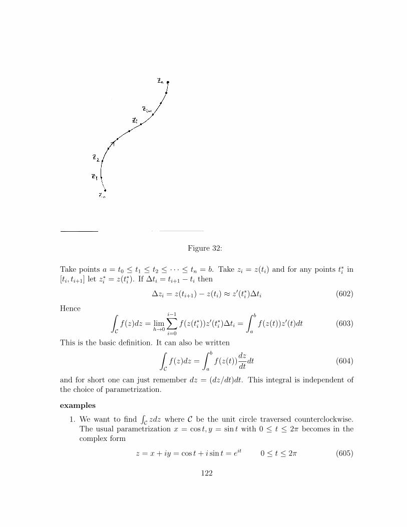
Figure 32:
Take points a = t0 ≤ t1 ≤ t2 ≤ · · · ≤ tn = b. Take zi = z(ti) and for any points t∗i in[ti, ti+1] let z∗i = z(t∗i ). If ∆ti = ti+1 − ti then
∆zi = z(ti+1)− z(ti) ≈ z′(t∗i )∆ti (602)
Hence ∫Cf(z)dz = lim
h→0
i−1∑i=0
f(z(t∗i ))z′(t∗i )∆ti =
∫ b
a
f(z(t))z′(t)dt (603)
This is the basic definition. It can also be written∫Cf(z)dz =
∫ b
a
f(z(t))dz
dtdt (604)
and for short one can just remember dz = (dz/dt)dt. This integral is independent ofthe choice of parametrization.
examples
1. We want to find∫C zdz where C be the unit circle traversed counterclockwise.
The usual parametrization x = cos t, y = sin t with 0 ≤ t ≤ 2π becomes in thecomplex form
z = x+ iy = cos t+ i sin t = eit 0 ≤ t ≤ 2π (605)
122

Thendz = ieitdt (606)
and so ∫Czdz =
∫ 2π
0
eitieitdt =
∫ 2π
0
ie2itdt =
[e2it
2
]2π
0
= 0 (607)
2. With the same curve C∫Czdz =
∫ 2π
0
e−itieitdt =
∫ 2π
0
idt = 2πi (608)
3. Let C = C1 + C2 where C1 is a straight line from 0 to 1 and C2 is a straight linefrom 1 to 1 + i. We evaluate∫
Czdz =
∫C1zdz +
∫C2zdz (609)
The line C1 is parametrized by z = t, 0 ≤ t ≤ 1. Hence dz = dt and z = t and∫C1zdz =
∫ 1
0
tdt =1
2(610)
The line C2 is parametrized by z = 1+it, 0 ≤ t ≤ 1. Hence dz = idt and z = 1−itand ∫
C1zdz =
∫ 1
0
(1− it)idt =
∫ 1
0
(i+ t)dt =
[it+
t2
2
]1
0
= i+1
2(611)
Thus∫C zdz = 1 + i.
3.10 properties of line integrals
To estimate the size of a line integral we have:
Theorem 27 Suppose a curve C has length L and |f(z)| ≤M for all z on C. Then∣∣∣∣∫Cf(z)dz
∣∣∣∣ ≤ML (612)
Proof. Approximate the integral by a sum∑
i f(z∗i )∆zi. By the triangle inequality∣∣∣∣∣∑i
f(z∗i )∆zi
∣∣∣∣∣ ≤∑i
|f(z∗i )∆zi|
=∑i
|f(z∗i )||∆zi|
≤M∑i
|∆zi|
(613)
123
Now take the limit as h = maxi |∆zi| → 0 and get the result.
example: Let C be a semi-circle of radius R in the upper half plane centered on theorigin. Suppose we want to estimate the size of
∫C(z + 1)3dz. For z on C we have
|(z + 1)3| = |z + 1|3 ≤ (|z|+ 1)3 = (R + 1)3 (614)
The length of C is πR. Hence by the theorem∣∣∣∣∫C(z + 1)3dz
∣∣∣∣ ≤ (R + 1)3πR (615)
Next we want to express our complex line integrals in terms of there real andimaginary parts. Start with the definition∫
Cf(z)dz =
∫ b
a
f(z(t))dz
dtdt (616)
where z(t), a ≤ t ≤ b is a parametrization of C. Then insert the expressions
f(z) =u(x, y) + iv(x, y)
z(t) =x(t) + iy(t)(617)
This gives ∫Cf(z)dz =
∫ b
a
(u(x(t), y(t)) + iv(x(t), y(t))
)(dxdt
+ idy
dt
)dt
=
∫ b
a
(u(x(t), y(t))
dx
dt− v(x(t), y(t))
dy
dt
)dt
+i
∫ b
a
(u(x(t), y(t))
dy
dt+ v(x(t), y(t))
dx
dt
)dt
=(∫Cudx− vdy
)+ i(∫Cudy + vdx
)(618)
For short one can think of making the substitutions f = u+ iv and dz = dx+ idy.This formula expresses complex line integrals in terms of real line integrals. From
this we can deduce that the complex line integrals have all the properties of real lineintegrals. In particular ∫
−Cf(z)dz = −
∫Cf(z)dz (619)
124
3.11 Cauchy’s theorem
Now we can prove:
Theorem 28 (Cauchy’s theorem) If f(z) is analytic everywhere inside a simple closedcurve C then ∫
Cf(z)dz = 0 (620)
Proof. Let R be the region inside C. Then by Green’s theorem followed by the CRequations: ∫
Cf(z)dz =
(∫Cudx− vdy
)+ i(∫Cvdx+ udy
)=
∫R
(− ∂v
∂x− ∂u
∂y
)dxdy + i
∫R
(∂u∂x− ∂v
∂y
)dxdy
=0
(621)
examples: Let C be the unit circle traversed counterclockwise. Then we have∫Czn dz =0 n = 0, 1, 2, . . .∫Cez dz =0∫
Cez
2+cos(3z) dz =0∫C
1
z − 2dz =0
(622)
since in each case the integrand is analytic inside the circle. But for integrals like∫Cezdz
∫C
1
z − 1/2dz
∫C
log z dz (623)
there is no conclusion since the integrand is not analytic inside the circle
We define a region as a connected open set.
Corollary If f is analytic inside a simply connected region D then∫Cf(z)dz = 0 for
any closed curve in D.
Proof. Suppose C is a simple closed curve. Since D is simply connected the interior ofC is in D, hence f is analytic inside C and the result follows by Cauchy’s theorem. IfC is not simple break it up into pieces which are simple.
125

Figure 33:
Corollary If f is analytic inside a simply connected region D then integrals∫Cf(z)dz
are independent of path in D.
Proof. If C1 and C2 are paths in D with the same endpoints then C1 − C2 is a closedcurve in D and so
∫C1 f −
∫C2 f =
∫C1−C2 f = 0 by the previous Corollary.
Corollary (deformation theorem) Let f be analytic in a region D and let C1, C2 besimple closed curves in D such that C1 can be continuously deformed to C2 in D. Then∫
C1f =
∫C2f (624)
Proof. We prove the result in the case where C1, C2 are simple closed curves and C1 isinside C2. The hypotheses of the theorem imply that f is analytic in the region betweenthem.
Let C be a curve which traverses C1, then jumps to C2 along a path γ, then traverses−C2, then jumps back to C1 along −γ. (see figure 33) Then C is a closed curve and fis analytic inside it and so by Cauchy’s theorem∫
C1f −
∫C2f =
∫C1f +
∫γ
f +
∫−C2
+
∫−γf =
∫Cf = 0 (625)
126
3.12 Cauchy integral formula
We need formulas for the direct evaluation of complex line integrals, i.e. without makinga parametrization. The first is a generalization of the fundamental theorem of caculus.
Theorem 29 Let f be analytic in a region D. Then∫C f′(z)dz is independent of path
in D and so can be written∫ z1z0f ′(z)dz. We have∫ z1
z0
f ′(z)dz = f(z1)− f(z0) (626)
Proof. Given points z0, z1 in D let C be any path from z0 to z1 and let z(t), a ≤ t ≤ bbe any parametrization of C with z(a) = z0 and z(b) = z1. Then by the chain rule∫
Cf ′(z)dz =
∫ b
a
f ′(z(t))z′(t)dt
=
∫ b
a
d
dt
[f(z(t)
]dt
=f(z(b))− f(z(a))
=z1 − z0
(627)
example: ∫ 1+i
0
z3dz =
[z4
4
]1+i
0
=(1 + i)4
4=
(√
2eiπ/4)4
4= eiπ = −1 (628)
To use the theorem one still has to find an anti-derivative for the integrand. Forclosed curves there is another formula which evaluates integrals with no work at all.
Theorem 30 (Cauchy Integral Formula) Let f(z) be analytic inside a simple closedcurve C traversed counterclockwise. Let z0 be a point inside C. Then∫
C
f(z)
z − z0
= 2πif(z0) (629)
Note that if z0 is outside C then f(z)/(z−z0) is analytic inside C and so the integralis zero by Cauchy’s theorem.
127
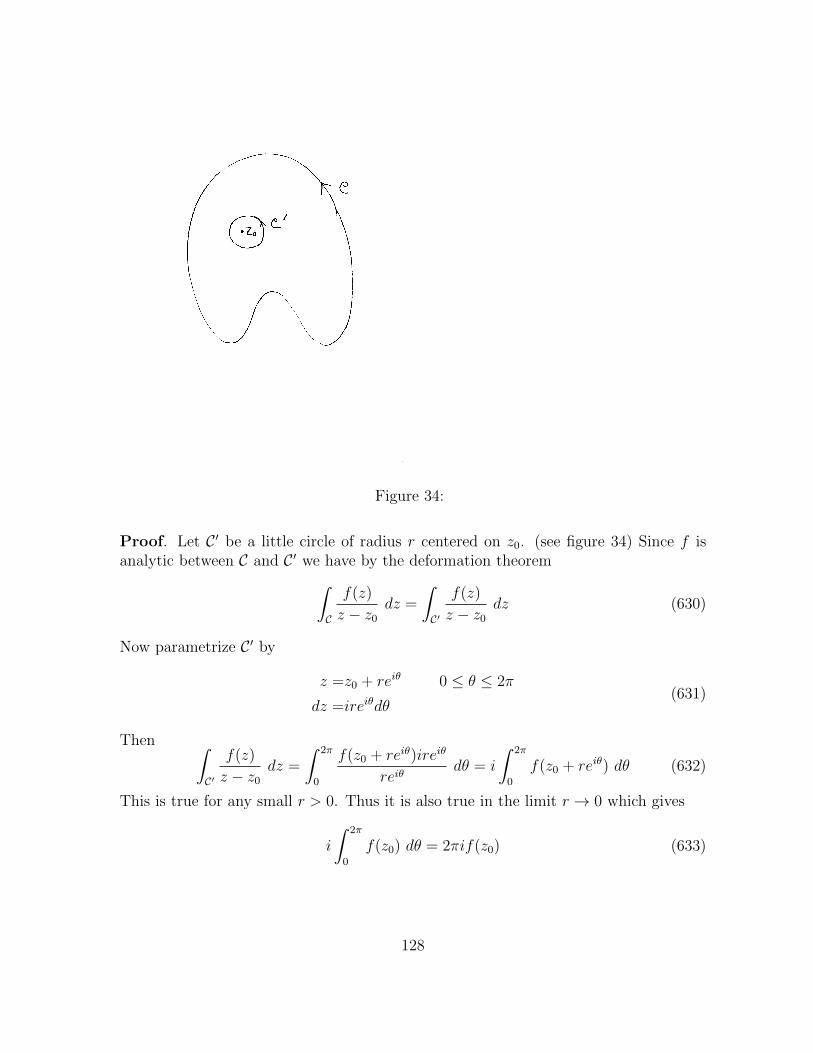
Figure 34:
Proof. Let C ′ be a little circle of radius r centered on z0. (see figure 34) Since f isanalytic between C and C ′ we have by the deformation theorem∫
C
f(z)
z − z0
dz =
∫C′
f(z)
z − z0
dz (630)
Now parametrize C ′ by
z =z0 + reiθ 0 ≤ θ ≤ 2π
dz =ireiθdθ(631)
Then ∫C′
f(z)
z − z0
dz =
∫ 2π
0
f(z0 + reiθ)ireiθ
reiθdθ = i
∫ 2π
0
f(z0 + reiθ) dθ (632)
This is true for any small r > 0. Thus it is also true in the limit r → 0 which gives
i
∫ 2π
0
f(z0) dθ = 2πif(z0) (633)
128

examples: Let C be the circle |z| = 2 traversed counterclockwise. Then∫C
ez
z − 1dz = 2πi[ez]z=1 = 2πie∫
C
ez
z − 3dz = 0∫
C
4z2 + 7
z − 1dz = 2πi[4z2 + 7]z=1 = 22πi
(634)
example: Let C be the square with corners i,−i, 2 − i, 2 + i traversed in that order.We want to evaluate ∫
C
ez
z2 − 1dz =
∫C
ez
(z + 1)(z − 1)dz (635)
The integrand goes bad at both z = ±1 but only z = 1 is inside C. Thus ez/(z + 1) isanalytic inside the curve and we can evaluate the integral as∫
C
ez/(z + 1)
z − 1dz = 2πi[ez/(z + 1)]z=1 = πie (636)
example: Let C be the circle |z| = 2 traversed counterclockwise. We want to evaluate∫C
ez
z2 + 1dz =
∫C
ez
(z + i)(z − i)dz (637)
The integrand goes bad at z = ±i and this time both points are inside C. Thus wecannot use the Cauchy integral formula as it stands. We give two methods to modifythe problem so that we can use it.
Solution (1). Break the denominator up using partial fractions We look for A,B suchthat
1
(z + i)(z − i)=
A
z − i+
B
z + i(638)
for all z. This is the same as
1 = A(z + i) +B(z − i) (639)
Matching coefficients gives A+B = 0 and Ai−Bi = 1. The solution is A = 1/2i andB = −1/2i. Therefore
1
(z + i)(z − i)=
1
2i
( 1
z − i− 1
z + i
)(640)
Inserting this into the integral it becomes
1
2i
∫C
ez
z − idz − 1
2i
∫C
ez
z + idz = 2πi
(ei − e−i
2i
)= 2πi sin(1) (641)
129

Figure 35:
Solution (2). Deform the curve to a pair of little circles C1 around z = i and C2 aroundz = −i. (see figure 35.) Then the integral is∫
C1
ez
(z + i)(z − i)dz +
∫C2
ez
(z + i)(z − i)dz
=2πi
[ez
z + i
]z=i
+ 2πi
[ez
z − i
]z=−i
=2πi
(ei − e−i
2i
)= 2πi sin(1)
(642)
130

3.13 higher derivatives
Let f be analytic in a region D, let z be a point in D, and let C be a simple closedcurve enclosing z such that the interior is contained in D, for example C could be alittle circle around z. By the Cauchy integral formula
f(z) =1
2πi
∫C
f(ζ)
ζ − zdζ (643)
The integrand here is a differentiable function of z since
d
dz
[1
ζ − z
]=
1
(ζ − z)2(644)
One can differentiate under the integral sign obtain
f ′(z) =1
2πi
∫C
f(ζ)
(ζ − z)2dζ (645)
Repeat the argument and conclude that f ′(z) is differentiable and that
f ′′(z) =2
2πi
∫C
f(ζ)
(ζ − z)3dζ (646)
Repeat the argument and conclude that f ′′(z) is differentiable and that
f ′′′(z) =3 · 22πi
∫C
f(ζ)
(ζ − z)4dζ (647)
In fact f can be differentiated any number of times and
f (n)(z) =n!
2πi
∫C
f(ζ)
(ζ − z)n+1dζ (648)
This is a remarkable result: assuming only f is analytic, i.e. once differentiable, weconclude that it is infinitely differentiable. This can certainly fail for functions of a realvariable.
The last formula can also be used to evaluate integrals. We replace z by z0 and ζby z and state it as follows.
Theorem 31 Let f be analytic inside a simple closed curve C traversed counterclock-wise. Let z0 be a point inside C. Then for n = 0, 1, 2, . . .∫
C
f(z)
(z − z0)n+1dz =
2πi
n!f (n)(z0) (649)
131

Notation: If C is a circle of radius r centered on z0 traversed counterclockwise then∫Cf(z)dz can be written
∮|z−z0|=r
f(z)dz (650)
examples ∮|z|=2
e6z
z − 1dz =2πi
[e6z]z=1
= 2πie6
∮|z|=2
e6z
(z − 1)2dz =
2πi
1!
[d
dze6z
]z=1
= 12πie6
∮|z|=2
e6z
(z − 1)3dz =
2πi
2!
[d2
dz2e6z
]z=1
= 36πie6
(651)
example∮|z|=1
sin(sin z)
z2dz = 2πi
[d
dzsin(sin z)
]z=0
= 2πi [cos(sin z) cos z]z=0 = 2πi (652)
3.14 Cauchy inequalities
Let C be a circle of radius R around a point a. Suppose that f(z) is analytic inside thecircle and that on the circle we have the bound
|f(z)| ≤M z ∈ C (653)
The Cauchy integral formula says that
f(a) =1
2πi
∫C
f(z)
z − adz (654)
We use this to estimate |f(a)|. For z on C we have∣∣∣∣ f(z)
z − a
∣∣∣∣ =|f(z)||z − a|
=|f(z)|R≤ M
R(655)
Then length of the curve is 2πR. Thus
|f(a)| ≤ 1
2π
M
R2πR = M (656)
We could take M to be the maximum of |f(z)| on the circle and then this says that |f |at the center of a circle is less than or equal to the maximum of |f | on the circle.
132

More generally we have
f (n)(a) =n!
2πi
∫C
f(z)
(z − a)n+1dz (657)
Now z on C we have ∣∣∣∣ f(z)
(z − a)n+1
∣∣∣∣ ≤ M
Rn+1(658)
and so
|f (n)(a)| ≤ n!
2π
M
Rn+12πR =
n!M
Rn(659)
We restate the result as a theorem.
Theorem 32 (Cauchy inequalities.) Let f be analytic inside a circle of radius R cen-tered on a and suppose |f | ≤M on the circle. Then for n = 0, 1, 2, . . .
|f (n)(a)| ≤ n!M
Rn(660)
This has some interesting consequences.
Theorem 33 (Liouville’s theorem) Suppose f is analytic in the entire plane and f isbounded, that is |f(z)| ≤M for some M and all z. Then f is constant.
Proof. f is analytic inside any circle of radius R centered on any a, and is boundedby M on the circle. By the n = 1 Cauchy inequality
|f ′(a)| ≤ M
Rfor all a,R (661)
Taking the limit R→∞ gives
|f ′(a)| ≤ 0 for all a (662)
Hence f ′(a) = 0 for all a and so f is a constant.
Theorem 34 (Fundamental theorem of algebra) Every polynomial P (z) of degree n ≥ 1has n roots (not necessarily distinct)
Proof. Suppose it is not true and P (z) 6= 0 for all z. Then 1/P (z) is analyticeverywhere. Furthermore if P (z) = anz
n + · · ·+ a1z + a0 with an 6= 0 then
limz→∞
1
P (z)= lim
z→∞
1
anzn + · · ·+ a1z + a0
= limz→∞
z−n
an + an−1z−1 · · ·+ a1z−n+1 + a0z−n
=0
an= 0
(663)
133

From this and the fact that 1/P (z) is continuous one can deduce that it is boundedThen by Liouville’s theorem 1/P (z) is constant and hence P (z) is constant. This is acontradiction. Thus we must have P (z) = 0 for some z. The polynomial has at leastone root.
If we call the root a1 then P (z) must have z − a1 as a factor so
P (z) = (z − a1)P1(z) (664)
where P1(z) is a polynomial of degree n− 1. Repeating the argument P1 must have aroot a2 and hence a factor z − a2. Then
P (z) = (z − a1)(z − a2)P2(z) (665)
where P2(z) has degree n − 2. After n steps we are left with n factors z − ai and apolynomial of degree 0 which is a constant c
P (z) = (z − a1)(z − a2) · · · (z − an)c (666)
This exhibits the n roots.
3.15 real integrals
The Cauchy integral formula is so easy to use that it is worthwhile going to a lot oftrouble to mold other integrals into this form. In particular this can be done for certainreal integrals.
Consider first integrals of the form∮|z|=1
f(z)dz. Parametrizing the unit circle by
z = eiθ, 0 ≤ θ ≤ 2π and dz = ieiθdθ we have∮|z|=1
f(z)dz =
∫ 2π
0
f(eiθ)ieiθdθ (667)
Now we reverse this process. Suppose we an integral of the form∫ 2π
0F (cos θ, sin θ)dθ
for some real function F . (Such integrals come up for example when computing Fourierseries.) Then we can write it a complex integral over the unit circle by∫ 2π
0
F (cos θ, sin θ)dθ
=
∫ 2π
0
F(eiθ + e−iθ
2,eiθ − e−iθ
2i
)ieiθdθieiθ
=
∫|z|=1
F(z + z−1
2,z − z−1
2i
)dziz
(668)
Thus the method is to make the substitutions
cos θ =z + z−1
2sin θ =
z − z−1
2idθ =
dz
iz(669)
134
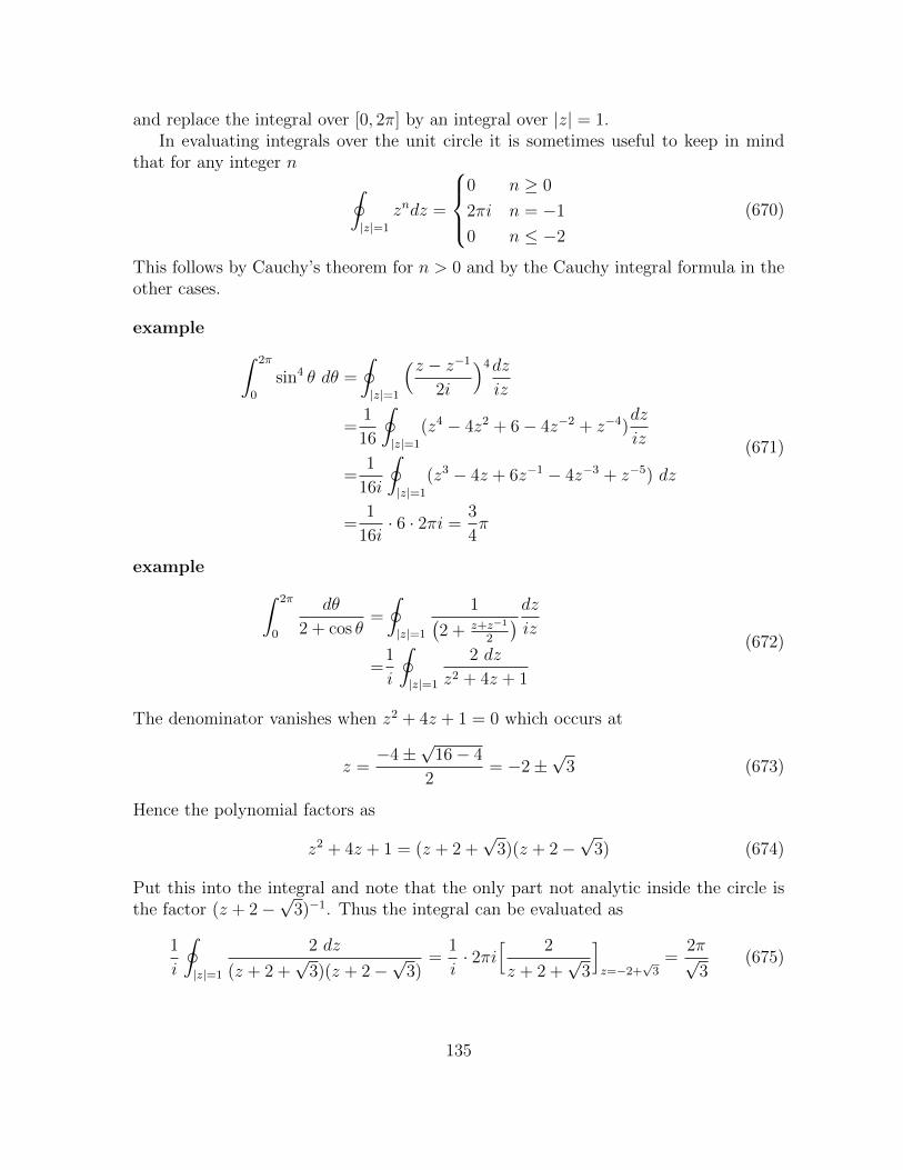
and replace the integral over [0, 2π] by an integral over |z| = 1.In evaluating integrals over the unit circle it is sometimes useful to keep in mind
that for any integer n ∮|z|=1
zndz =
0 n ≥ 0
2πi n = −1
0 n ≤ −2
(670)
This follows by Cauchy’s theorem for n > 0 and by the Cauchy integral formula in theother cases.
example ∫ 2π
0
sin4 θ dθ =
∮|z|=1
(z − z−1
2i
)4dz
iz
=1
16
∮|z|=1
(z4 − 4z2 + 6− 4z−2 + z−4)dz
iz
=1
16i
∮|z|=1
(z3 − 4z + 6z−1 − 4z−3 + z−5) dz
=1
16i· 6 · 2πi =
3
4π
(671)
example ∫ 2π
0
dθ
2 + cos θ=
∮|z|=1
1(2 + z+z−1
2
) dziz
=1
i
∮|z|=1
2 dz
z2 + 4z + 1
(672)
The denominator vanishes when z2 + 4z + 1 = 0 which occurs at
z =−4±
√16− 4
2= −2±
√3 (673)
Hence the polynomial factors as
z2 + 4z + 1 = (z + 2 +√
3)(z + 2−√
3) (674)
Put this into the integral and note that the only part not analytic inside the circle isthe factor (z + 2−
√3)−1. Thus the integral can be evaluated as
1
i
∮|z|=1
2 dz
(z + 2 +√
3)(z + 2−√
3)=
1
i· 2πi
[ 2
z + 2 +√
3
]z=−2+
√3
=2π√
3(675)
135
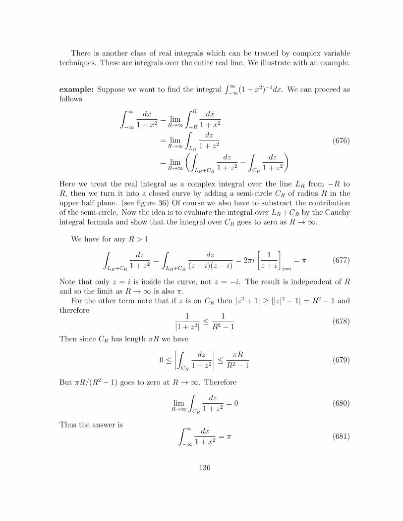
There is another class of real integrals which can be treated by complex variabletechniques. These are integrals over the entire real line. We illustrate with an example.
example: Suppose we want to find the integral∫∞−∞(1 + x2)−1dx. We can proceed as
follows ∫ ∞−∞
dx
1 + x2= lim
R→∞
∫ R
−R
dx
1 + x2
= limR→∞
∫LR
dz
1 + z2
= limR→∞
(∫LR+CR
dz
1 + z2−∫CR
dz
1 + z2
) (676)
Here we treat the real integral as a complex integral over the line LR from −R toR, then we turn it into a closed curve by adding a semi-circle CR of radius R in theupper half plane. (see figure 36) Of course we also have to substract the contributionof the semi-circle. Now the idea is to evaluate the integral over LR +CR by the Cauchyintegral formula and show that the integral over CR goes to zero as R→∞.
We have for any R > 1∫LR+CR
dz
1 + z2=
∫LR+CR
dz
(z + i)(z − i)= 2πi
[1
z + i
]z=i
= π (677)
Note that only z = i is inside the curve, not z = −i. The result is independent of Rand so the limit as R→∞ is also π.
For the other term note that if z is on CR then |z2 + 1| ≥ ||z|2 − 1| = R2 − 1 andtherefore
1
|1 + z2|≤ 1
R2 − 1(678)
Then since CR has length πR we have
0 ≤∣∣∣∣∫CR
dz
1 + z2
∣∣∣∣ ≤ πR
R2 − 1(679)
But πR/(R2 − 1) goes to zero at R→∞. Therefore
limR→∞
∫CR
dz
1 + z2= 0 (680)
Thus the answer is ∫ ∞−∞
dx
1 + x2= π (681)
136

Figure 36:
3.16 Fourier and Laplace transforms
(A.) If f(x) is a function defined for −∞ < x < ∞, the Fourier transform of f is anew function f defined by
f(k) =
∫ ∞−∞
eikxf(x) dx (682)
The function can be recovered from its Fourier transform by the inversion formula
f(x) =1
2π
∫ ∞−∞
e−ikxf(k) dk (683)
Fourier transforms are useful for solving partial differential equations on the whole line,among other things. Complex integration techniques are useful for computing Fouriertransforms.
137

example: Suppose we want to find the Fourier transform of the function (1 + x2)−1.We proceed as in the last example∫ ∞
−∞
eikx
1 + x2dx = lim
R→∞
∫ R
−R
eikx
1 + x2dx
= limR→∞
∫LR
eikz
1 + z2dz
= limR→∞
(∫LR+CR
eikz
1 + z2dz −
∫CR
eikz
1 + z2dz
) (684)
Suppose that k > 0. Then for z = x + iy on the semi-circle CR we have y > 0 and so|eikz| = |eikx||e−ky| = e−ky ≤ 1. From before |1 + z2| ≥ R2 − 1 and so on CR∣∣∣∣ eikz1 + z2
∣∣∣∣ ≤ 1
R2 − 1(685)
Then ∣∣∣∣∫CR
eikz
1 + z2dz
∣∣∣∣ ≤ πR
R2 − 1→ 0 as R→∞ (686)
There is no contribution from the integral over CR.On the other hand by the Cauchy integral formula since z = i is inside the curve
and z = −i is not∫LR+CR
eikz
1 + z2dz =
∫LR+CR
eikz
(z + i)(z − i)dz = 2πi
[eikz
z + i
]z=i
= πe−k (687)
This holds for any R > 1 and hence also in the limit R→∞ and so∫ ∞−∞
eikx
1 + x2dx = πe−k k > 0 (688)
This analysis fails if k < 0 since then |eikz| = e−ky grows exponentially in y and wecannot argue that the contribution from CR vanishes. Instead we close the curve witha semi-circle C ′R in the lower half plane. We have∫ ∞
−∞
eikx
1 + x2dx = lim
R→∞
(∫LR+C′R
eikz
1 + z2dz −
∫C′R
eikz
1 + z2dz
)(689)
For z = x+ iy on C ′R we have y < 0 and so |eikz| = e−ky < 1 for k < 0. Then again∣∣∣∣∣∫C′R
eikz
1 + z2dz
∣∣∣∣∣ ≤ πR
R2 − 1→ 0 as R→∞ (690)
and there is no contribution from C ′R.
138
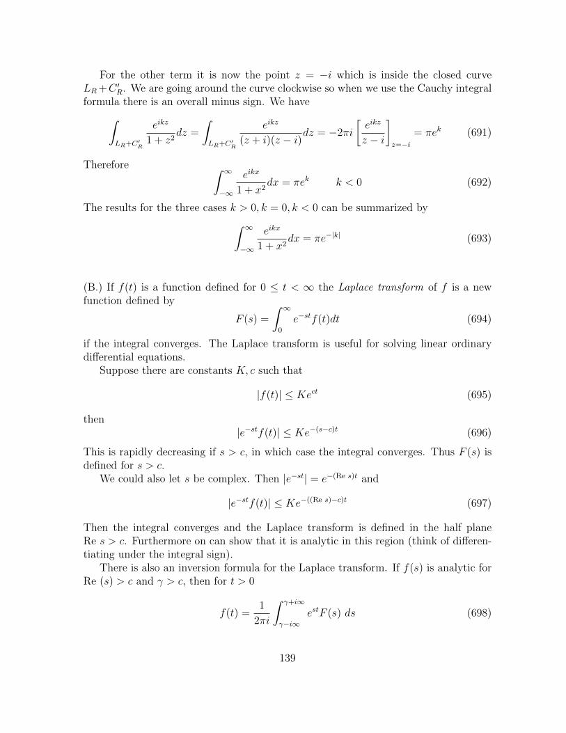
For the other term it is now the point z = −i which is inside the closed curveLR +C ′R. We are going around the curve clockwise so when we use the Cauchy integralformula there is an overall minus sign. We have∫
LR+C′R
eikz
1 + z2dz =
∫LR+C′R
eikz
(z + i)(z − i)dz = −2πi
[eikz
z − i
]z=−i
= πek (691)
Therefore ∫ ∞−∞
eikx
1 + x2dx = πek k < 0 (692)
The results for the three cases k > 0, k = 0, k < 0 can be summarized by∫ ∞−∞
eikx
1 + x2dx = πe−|k| (693)
(B.) If f(t) is a function defined for 0 ≤ t < ∞ the Laplace transform of f is a newfunction defined by
F (s) =
∫ ∞0
e−stf(t)dt (694)
if the integral converges. The Laplace transform is useful for solving linear ordinarydifferential equations.
Suppose there are constants K, c such that
|f(t)| ≤ Kect (695)
then|e−stf(t)| ≤ Ke−(s−c)t (696)
This is rapidly decreasing if s > c, in which case the integral converges. Thus F (s) isdefined for s > c.
We could also let s be complex. Then |e−st| = e−(Re s)t and
|e−stf(t)| ≤ Ke−((Re s)−c)t (697)
Then the integral converges and the Laplace transform is defined in the half planeRe s > c. Furthermore on can show that it is analytic in this region (think of differen-tiating under the integral sign).
There is also an inversion formula for the Laplace transform. If f(s) is analytic forRe (s) > c and γ > c, then for t > 0
f(t) =1
2πi
∫ γ+i∞
γ−i∞estF (s) ds (698)
139

Figure 37:
Here the integral is over the verticle line Re (s) = γ. Such lines can be deformed toeach other in the region of analyticity, so it does not matter what γ we take.
problem: Find the function whose Laplace tranform is (s− 2)−3
solution: The function is analytic for Re(s) > 2 so the function is is given by theinversion formula with γ > 2. We evaluate it by closing the curve in the left half plane:
f(t) =1
2πi
∫ γ+i∞
γ−i∞
est
(s− 2)3ds
= limR→∞
1
2πi
∫ γ+iR
γ−iR
est
(s− 2)3ds
= limR→∞
1
2πi
∫LR
est
(s− 2)3ds
= limR→∞
(1
2πi
∫LR+CR
est
(s− 2)3ds− 1
2πi
∫CR
est
(s− 2)3ds
)(699)
Here LR is the strait line from γ − iR to γ + iR and CR is the semi-circle of radius Rcentered on γ, see figure 37.
140

Now for s on CR we have Re(s) ≤ γ and so |est| = eRe(s)t ≤ eγt. Also the point onCR closest to 2 is γ −R and so |s− 2| ≥ |2− (γ −R)|. Therefore∣∣∣∣ 1
2πi
∫CR
est
(s− 2)3ds
∣∣∣∣ ≤ 1
2π
eγt
|2− (γ −R)|3· πR→ 0 as R→∞ (700)
The integral over CR does not contribute.If R is large enough, then the point 2 is inside LR + CR and so by the higher
derivative Cauchy integral formula
1
2πi
∫LR+CR
est
(s− 2)3ds =
1
2!
d2
ds2[est]s=2 =
1
2t2e2t (701)
This also holds in the limit R→∞ and so this answer is f(t) = 12t2e2t.
141