lecture 7 linear regression diagnosticscourses.washington.edu/b515/l7.pdf · lecture 7 linear...

Lecture 7Linear Regression Diagnostics

BIOST 515

January 27, 2004

BIOST 515, Lecture 6

Major assumptions

1. The relationship between the outcomes and the predictors is

(approximately) linear.

2. The error term ε has zero mean.

3. The error term ε has constant variance.

4. The errors are uncorrelated.

5. The errors are normally distributed or we have an adequate

sample size to rely on large sample theory.

We should always check fitted models to make sure that these

assumptions have not been violated.

BIOST 515, Lecture 6 1

Departures from the underlying assumptions cannot be de-

tected using any of the summary statistics we’ve examined so

far such as the t or F statistics or R2. In fact, tests based on

these statistics may lead to incorrect inference since they are

based on many of the assumptions above.


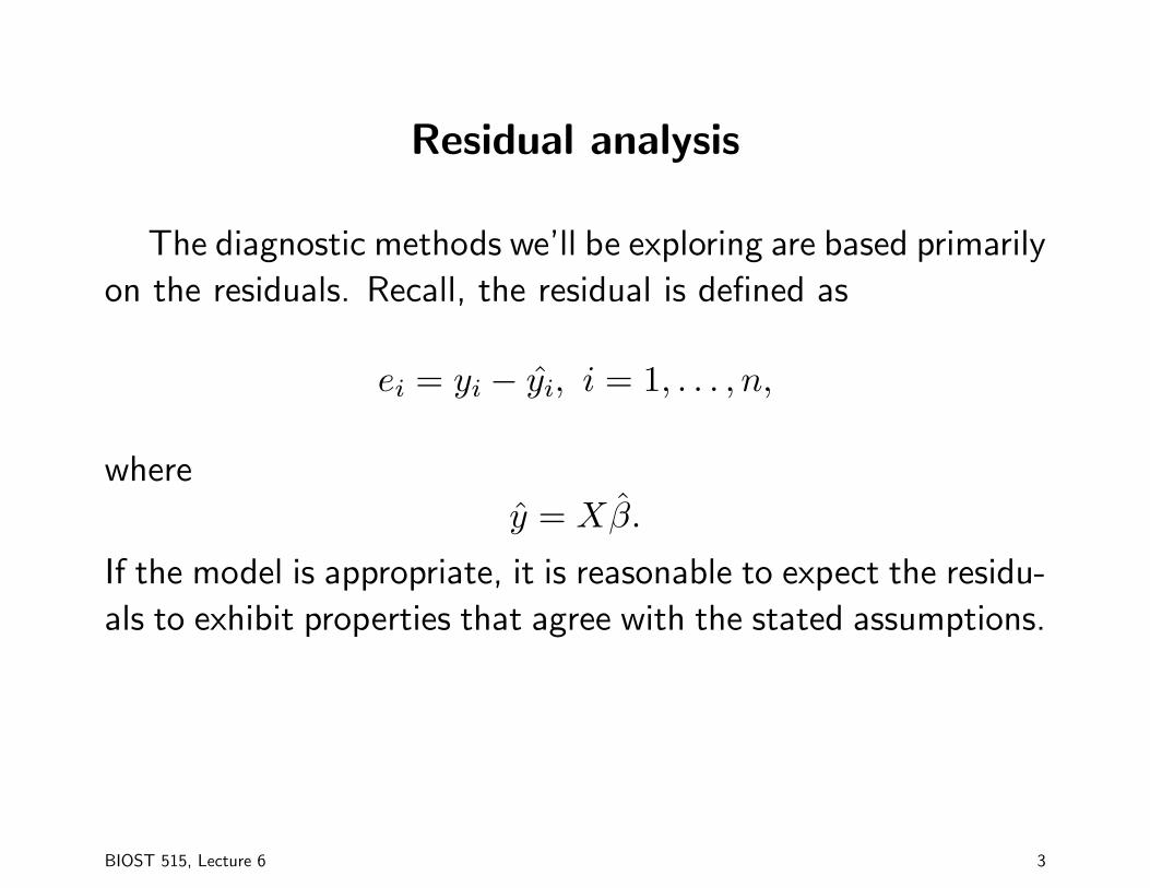
Residual analysis

The diagnostic methods we’ll be exploring are based primarily

on the residuals. Recall, the residual is defined as

ei = yi − yi, i = 1, . . . , n,

where

y = Xβ.

If the model is appropriate, it is reasonable to expect the residu-

als to exhibit properties that agree with the stated assumptions.


Characteristics of residuals

• The mean of the {ei} is 0:

e =1n

n∑i=1

ei = 0.

• The estimate of the population variance computed from the

sample of the n residuals is

S2 =1

n− p− 1

n∑i=1

e2i

which is the residual mean square, MSE = SSE/(n−p−1).


• The {ei} are not independent random variables. In general,

if the number of residuals (n) is large relative to the number

of independent variables (p), the dependency can be ignored

for all practical purposes in an analysis of residuals.


Methods for standardizing residuals

• Standardized residuals

• Studentized residuals

• Jackknife residuals


Standardized residuals

An obvious choice for scaling residuals is to divide them by

their estimated standard error. The quantity

zi =ei√

MSE

is called a standardized residual. Based on the linear re-

gression assumptions, we might expect the zis to resemble a

sample from a N(0, 1) distribution.


Studentized residuals

Using MSE as the variance of the ith residual ei is only an

approximation. We can improve the residual scaling by dividing

ei by the standard deviation of the ith residual. We can show

that the covariance matrix of the residuals is

var(e) = σ2(I −H).

Recall H = X(X ′X)−1X ′ is the hat matrix. The variance of

the ith residual is

var(ei) = σ2(1− hi),

where hi is the ith element on the diagonal of the hat matrix

and 0 ≤ hi ≤ 1.


The quantity

ri =ei√

MSE(1− hi)

is called a studentized residual and approximately follows a t

distribution with n − p − 1 degrees of freedom (assuming the

assumptions stated at the beginning of lecture are satisfied).

Studentized residuals have a mean near 0 and a variance,

1n− p− 1

n∑i=1

r2i ,

that is slightly larger than 1. In large data sets, the standardized

and studentized residuals should not differ dramatically.


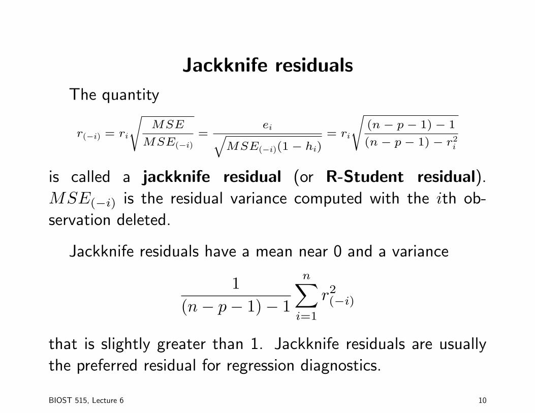
Jackknife residuals

The quantity

r(−i) = ri

sMSE

MSE(−i)

=eiq

MSE(−i)(1 − hi)= ri

s(n − p − 1) − 1

(n − p − 1) − r2i

is called a jackknife residual (or R-Student residual).MSE(−i) is the residual variance computed with the ith ob-

servation deleted.

Jackknife residuals have a mean near 0 and a variance

1(n− p− 1)− 1

n∑i=1

r2(−i)

that is slightly greater than 1. Jackknife residuals are usually

the preferred residual for regression diagnostics.


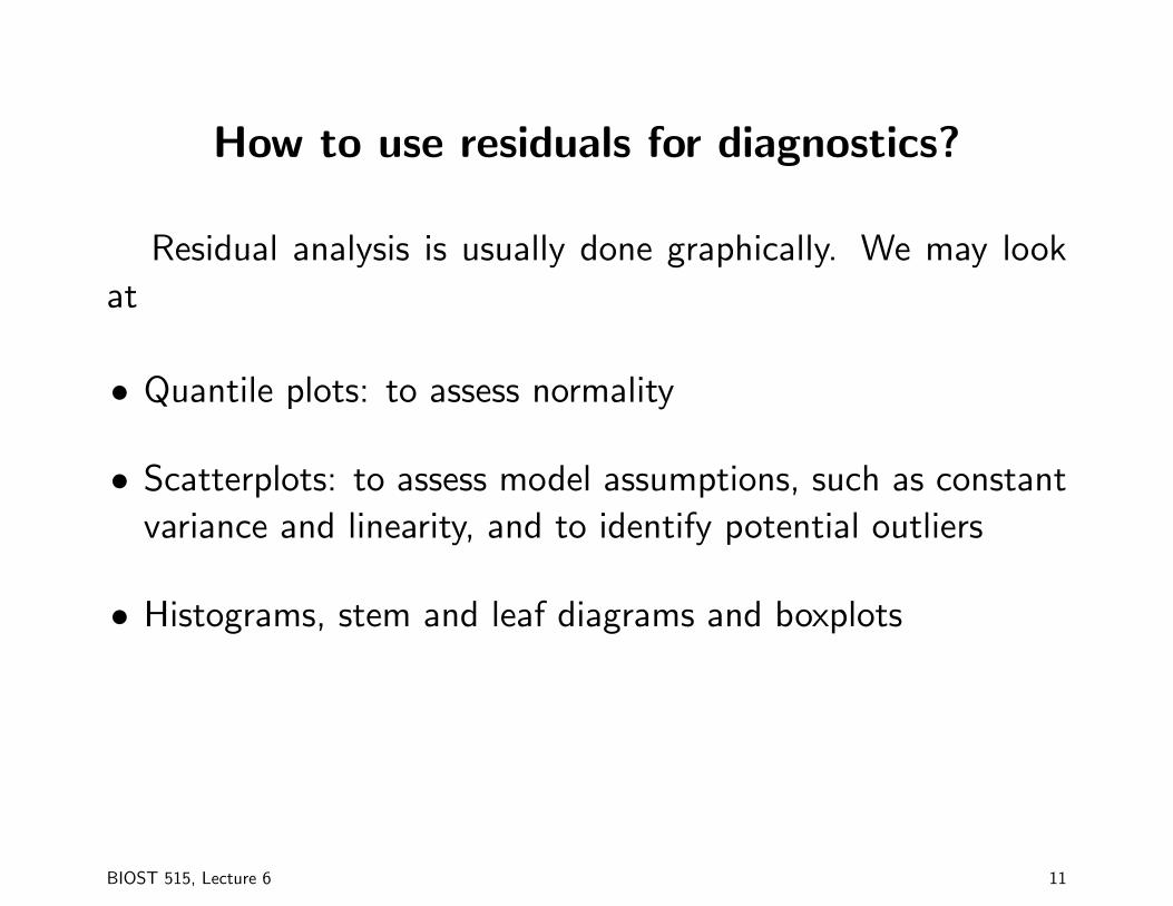
How to use residuals for diagnostics?

Residual analysis is usually done graphically. We may look

at

• Quantile plots: to assess normality

• Scatterplots: to assess model assumptions, such as constant

variance and linearity, and to identify potential outliers

• Histograms, stem and leaf diagrams and boxplots


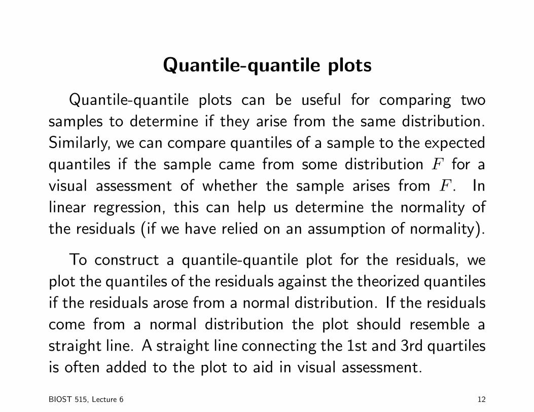
Quantile-quantile plots

Quantile-quantile plots can be useful for comparing two

samples to determine if they arise from the same distribution.

Similarly, we can compare quantiles of a sample to the expected

quantiles if the sample came from some distribution F for a

visual assessment of whether the sample arises from F . In

linear regression, this can help us determine the normality of

the residuals (if we have relied on an assumption of normality).

To construct a quantile-quantile plot for the residuals, we

plot the quantiles of the residuals against the theorized quantiles

if the residuals arose from a normal distribution. If the residuals

come from a normal distribution the plot should resemble a

straight line. A straight line connecting the 1st and 3rd quartiles

is often added to the plot to aid in visual assessment.


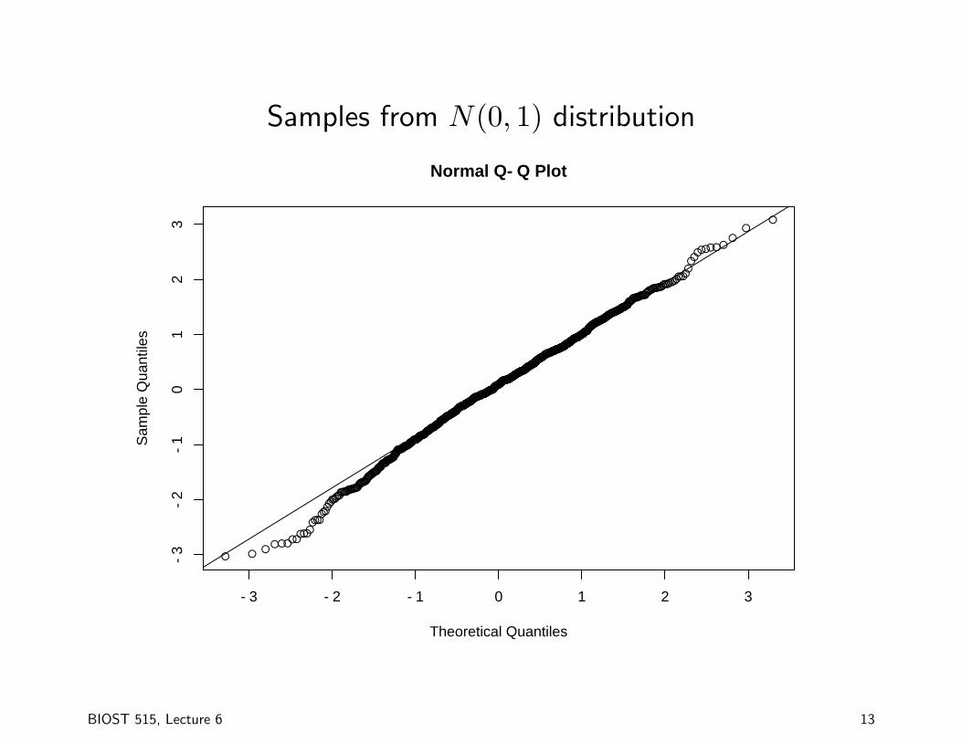
Samples from N(0, 1) distribution

●

●

●

●

●

●●

●

●

●

●

●●

●

●

●●●

●

●

●

●

●

●

●●

●

●

●

●

●

●

●

●

●

●

●

●●

●

●

●

●

●

●

●

●●

●

●

●

●

●

●

●

●

●

●

●

●

●●

●

●●

●

●●

●

●●

●

●

●

●

●

●

●

●

●

●

●

●

●

●

●

●

●

●

●

●

●

●

●

●

●

●

●

●

●

●

●

●

●

●

●

●

●

●

●

●

●

●

●●

●

●

●

●

●

●

●

●

●

●

●●

●

●

●

●●

●

●●

●

●●

●

●

●

●

●

●

●●

●●

●

●

●

●

●●

●●

●

●

●

●

●

●

●

●

●

●●●

●

●

●●

●

●

●

●

●

●

●

●

●

●●

●

●

●

●

●

●

●

●●

●

●

●

●●

●

●●

●

●

●

●●

●

●

●

●●

●

●

●

●

●●

●

●

●

●

●

●

●

●

●

●●

●

●

●

●●

●

●

●

●

●

●

●●

●

●

●

●

●

●

●

●

●

●

●

●●

●

●●

●

●

●●

●

●

●

●●

●

●

●

●

●

●

●

●

●

●

●

●

●

●

●

●

●

●

●

●

●

●

●

●

●

●

●●

●

●

●●

●

●

●

●

●

●

●

●

●

●

●

●

●

●

●

●

●

●

●

●

●

●

●●

●

●

●

●

●

●

●

●

●

●

●

●

●

●

●

●

●

●

●

●

●

●

●

●

●

●●

●

●

●

●

●

●●

●

●

●

●

●

●

●

●

●

●

●

●

●

●

●

●

●

●

●

●

●

●

●

●

●

●

●

●

●

●

●

●

●

●

●

●

●

●

●

●

●

●

●

●

●

●

●

●

●●

●

●

●●

●

●

●

●●

●

●

●

●

●

●

●

●

●

●

●

●

●

●

●

●

●

●

●●

●

●

●●

●

●●

●

●

●

●●

●

●

●

●

●

●

●

●

●

●

●

●

●

●

●

●

●

●

●

●

●

●

●

●

●

●

●

●●

●

●

●

●●

●

●

●

●

●

●●

●

●

●

●

●

●

●

●

●●●

●

●

●●

●

●●

●

●

●

●

●

●

●

●

●

●

●

●

●

●●

●

●

●

●

●

●●

●

●

●

●

●

●

●

●

●

●

●

●

●

●

●

●

●

●

●

●

●

●

●

●

●

●

●

●

●

●

●

●

●●

●

●

●

●

●

●

●●

●

●

●

●●

●

●

●

●

●

●

●

●

●

●

●●

●

●

●

●

●

●

●

●

●

●

●

●

●●

●

●●

●

●

●

●

●

●

●

●

●

●●●

●

●

●

●

●

●

●

●

●

●●

●

●

●

●

●

●

●

●

●

●

●

●

●●

●

●

●

●

●

●

●

●

●

●

●

●

●●

●

●

●

●

●

●

●

●

●

●

●

●●

●

●●

●

●

●

●

●

●

●

●

●

●

●

●

●

●

●

●

●

●

●

●

●

●

●

●

●

●

●

●

●

●●●

●

●

●

●

●

●

●

●

●

●

●

●

●

●

●

●

●

●●

●

●

●

●

●

●

●●

●

●

●

●

●

●

●●

●

●

●●

●

●

●

●●

●

●●

●●

●●

●

●●

●

●

●

●

●

●

●

●●

●

●●

●●

●

●

●●

●

●

●

●

●

●

●●

●

●

●

●

●

●

●●

●

●

●

●

●

●

●

●

●

●

●

●

●

●

●

●

●

●

●

●

●

●

●

●

●

●

●

●

●

●

●●

●●

●

●

●●

●

●

●

●

●

●

●

●

●

●

●

●●●

●

●

●

●

●●

●

●

●

●

●

●

●

●

●

●

●

●●

●

●●

●

●●

●

●

●

●

●

●●

●

●

●

●

●

●

●●

●

●

●

●

●

●

●●

●

●

●

●●

●

●●

●

●

●

●

●

●

●

●

●

●

●

●

●

●

●

●

●

●

●

●●

●

●

●

●

●

●

●

●

●●

●

●

●

●

●

●

●

●

●

●

●

●

●

●

●

●

●●

●

●

●

●

●

●

●

●

●

●

●

●

●

●●

●

●●

●

●

●

●●

●

●

●

●

●●

●

●

●

●

●

●

●

●

●

●

●

●

●

●

●

●

●

●

●

●

●

●

●

●

−3 −2 −1 0 1 2 3

−3

−2

−1

01

23

Normal Q−Q Plot

Theoretical Quantiles

Sam

ple

Qua

ntile

s


Samples from a skewed distribution

●

●●

●

●●

●●

●

●

●●●●

●

●

●

●

●

●●

●●

●●

●

●●

●

●

●●●

●

●

● ●

●

●●

●●

●

●

●

●

●

●

●●

●

●

●●

●

● ●●

●●

●

●●●● ● ●

●● ● ●

●

●●

●

●

●

●●

●●

●

●

●

●●

● ●

●

●●

●●

●

●

●

●

●

●

●●●

●

●

●●

●●●

●

●●

●

●

●

●

●

●●

●

●

●

●

●●

●●

●

●

●

●

●

●●

●

●

●●

●

●

●

●●

●

●●

●

●

●

●●

●●

●

●

● ●● ●

●

●●

●

●

●●

●●

●

●

●●

●

●

●

●●

●

●

●

●

●●

●

●●

●

●● ●

● ●

●

●

●

●● ●

●

●

●

●●

●●●

●●●●● ●

●

●

●●

●

●●

●

●

●

● ●

●

●

●

●

●●●

●●

●

●●

●●●

●

●●●

●

●●

●●

●

●

●

●●

●●●●

●●

●

●●

●

●

● ●

●

●

●●

●

●

●

●

●●

●

●

●●

●

●

●

●

●

●

●●

●

●

●●

●

●●

●

●

●

●●

●●

●

●

●

●

●

●●

●

●●

●

●

●●

●

●

●

●●

●

●

●

●

●

●

●

●

●

●●

●

●

●●

●●

● ●●

●

●

●●

●●

●●

●

●●

●

●

●

●

●

●●

●

●

●●

●

●●

●●● ●

●

●

●

●

●

●

●

●

●

●●

●●

●

●

●

●

●●●

●

●

●

●

●

●●●

●

●

●

●●●●

●●●●

●

●

●

●

●

●● ●

●●

●●

●●

●

●

●

●

●●

●●

● ●

●●●

●

●●●

● ●●●

●

●

●

●● ●

●

●

●●

●●

●

●●

● ●●●

●

●

●

●

●

●

●

●●

● ●●

●

●●

●

●●●

●●● ●

●●●●

●● ●●

●

●

●

●

●●

●

●

●

●

●

●●

●

●● ●

●●

● ●●

●●●

●●

●

●

● ●

●

●●

●

●

●●

●

●●

●●

●

●

●●

●●

●

●

● ●

●

●

●●

●

●●

●

●●

●

● ●

●

●

●●●

●

●●●

●

●●

● ●

●

●

●●●

●●

●

●●

●

●

●

●●

● ●●

●

●● ●●

●● ●

●●

●●●

● ●●

●● ●

●

●

●

●

●

●●

●

●

● ●

●

●

●●

●

●●

● ●●●●

● ●

●

●

●●

●

●●●

●

●

●●

●●

●

●●

●●

●●●

●

●

●

●

●● ●

●

● ●

●

●

●●●●

●

●●●

●●

●

●

●●

●

●●●

●●

●

●

●● ●●

●●●

●●●

●

●

●

●●

●

●●●

●

●

●

●

●

●

●

●

●

●

●●

●

●●

●

●

●●

●●

●●

●

●

●

●

●

●

●

●

●●

●

●●

●●

●

●

● ●●

●

●●

●●●

●

● ●●

●

●●

●●●

●

●●

●

●

●

●●

●● ●

●●

●

●

●●

●

●

●●

●●

● ●●

●

●●

● ●●

●

●●

● ●

● ●

●

● ●●

●

●

●● ●

●

●●

●

●

●

●●

●

● ● ●

●

●

●

●

●●

●

●

●

●

●

●●

●

●

●

●●

●●●●

● ●

●

●

●●

●●

●

●

●

●

●

●

●

●

●

●●

●

●

●

●●

●

●

●

●●●

●

●●

●

●●●

●

●

●

●

●

●

●

●

●●●

● ●● ●●

●

●

●

●

●

●

●

●●●●

●

● ●

●●

● ●

●

●

● ●

●

●

●●

●●

●

●●

●

●●

●●

●

●

●

●●

●

●

●●●

●●●

●

●●

●●

●●●

●

●

●●

●

●

●●

●

●

●

●●

● ●●

●

●

● ●

●●

●●

●

●●

● ●

●

●● ●

●●●

●●

−3 −2 −1 0 1 2 3

−2

02

4Normal Q−Q Plot


Res

idua

ls

Histogram of y

Residuals

Den

sity

−2 −1 0 1 2 3 4

0.0

0.2

0.4


Samples from a heavy-tailed distribution

●●

●●

● ● ●

●●

●

●●

●● ●●

●●●

●

●

●● ●● ●●

●●

●

●●

●●

●●

●

●

●●●●

●●

●●●

●

●

●●●

● ●

●●

●●●

●●

●●●●

●

● ●●●●

●

●●● ●

●

●●●

● ●● ●

● ●●●

● ●●

●

●

● ● ●●●

●

●● ● ● ●●●● ●● ●

●●

● ●

●●

●

●●●

●● ●●

●●

●●

●● ●

●●●●● ●● ●● ● ●

●●

●● ●●

●

●

● ●●

●

● ●●

● ●●●●●●●● ●

●

●

●

●●

●●

●●

● ● ●●●

●●● ●

●●● ●

●●

●

●

●●

●●

●● ●●

●● ●

●● ●●

● ●●

● ●●

●●● ●●● ●●●●

●●

●

●

●●●

● ●●

●

●●

●●●●●● ●●● ● ●● ● ●

●●

● ●● ●

●

●●

●●●

●

●●

●●

● ● ●● ●● ●

●

●

●●

●

●●●

● ● ●●●● ●

● ● ●●●●

●●

● ● ●●●●

●●

●●

●●

●

●●● ●●

●●

●●

●●●●●

●●

●

●

●●

●●

●

●

●

●●●

●●●

●●●

●● ●●●

●● ●●

●

●●

● ●● ●●

●●●

●● ● ●

●

●

●● ●● ●

●●●

●●●●●

●●●●

●●

●

●●● ●●● ●●

●

●● ●● ●

● ●●

●● ●●●●

●

●●●

●

●

●

●

●

●● ●

● ●●● ●

●●

● ●

●●

●●

●

● ●●● ● ●

●

● ●● ●

●● ● ●●

●●

●

● ●●●●

●●●● ●● ●

●● ●● ●

● ● ●●●●

●●

●

●●●

●● ●

●

●● ●●●

●

●

●●

●● ●

●●

●●

●●

●

●

●●●●

●●

●●●● ● ●

●

●●● ●●●

● ●●

●●● ●● ●● ●● ● ●●●●

●●

●●

●●●●● ●●

● ●●● ●●●●●

●●

●●

●

●

● ●●●

●●● ●●

● ●●

●

●

●●

● ●●

● ●●●

●●●

● ●●

●●

●●

●

●

●●

● ●●

●●●●●●

●

●

●

●●

●●

●●●

●●

●

●

●●

● ●●

●●

●

●●

●

●● ●●

●● ●●

●●●

●●

● ●●

●●●

●● ●

●●

●

●

●●

●● ● ●●

●●● ●●●● ●

●

●●●●

●●● ●

●●

●●

●

●

●

●

●●●● ●

●

●●

●

●●

●●●

● ●● ● ●●

●

●●● ●

● ●●

●●

●● ●●

●

●

●●

●●

●●●

●

●

● ●

●

● ●●

●●●

●

●●●

●

●●● ●

●●●

●●

●●

● ●●

●●● ●●

●

●●

●● ●

●

●●

●● ●●

●

●

●●●●●●●● ● ● ● ●

●●

●●

●● ● ●●

●

●

●●●

●

●● ● ● ●●

●●

● ● ● ●●

● ●

●

●

●●●●

●●

●●

●

●

●●

●●

● ●● ●●● ●

●●

●●●

● ●

●

● ●

●

●●●

●● ●

●● ●●

● ●●

●●

●

●

●

●

●●

●●

●●

●●● ● ●

●●●● ●●●●

●●● ●

●

●●● ●

●

● ●●

●●

●● ●●●

●

●●● ●

●

●●●●

● ●●●● ●●

●

●

● ●●

●●●

●●

●●●

●●

●

●●

●●●●●

●●●

●●

●

● ● ●●● ●● ●●

●● ●

●

●● ●

●● ●

●●

●●●

−3 −2 −1 0 1 2 3

−4

04

8Normal Q−Q Plot


Res

idua

ls

Histogram of y

Residuals

Den

sity

−4 −2 0 2 4 6 8

0.0

0.3

0.6


Samples from a light-tailed distribution

●●

●

●●

●●

●

●●

●

●

●

●●

●

●

●

●

●

●●

●

●

●

●●

●

●●

●●

●

●

●

●

● ●

●●

●

●

●

●

●

●●

●●

●

●

●●

●

●

●

●

●

●●

●

●

●

●

● ●

●

●●

●

●

●●

●

●

●

●

●●

●

●●

●

●

●

●

●

●

●● ●

●

●

●

●

●

●●

●

●●

●

●

●●

●●

●

●

●

●

●

●

● ●

●●

●

●●●

●●

●

●

●

●●

●

●

●

●

●

●●

●

●

●

●

●

●

●

●

●

●●

●

●

●

●

●

●

●

●

●

●

●

●

● ●●

●●

●

●

●●

●

●●

●

●

●

●

●

●●

●

●

●

●●

●●

●

●

●●

●

●

●

●●

●

●

●●

●

●

●

●

●●

● ●

●

●

●

●

●

●●

●●

●●

●

●

●

●

●

●

●

●●

●

●

●●

●

●

●●

●

●

●

●

●

●

●

●

●

●

●

●●●

●

●

●

●

●

●

●

●

●

●

●

●

●

●

●

●

●

●●

●

●

●●

●

●●●

●

●●

●

●●

●

●

●

●

●

●

●●

●

●

●

●

●●

●

●

●

●●

●

●

●

●●●

●

●

●

● ●

●●

●

●●

●

●●

●

●

●●

●●●

●

●

●●

●●

●● ●

●

●

●

●

●

●

●●

●●

●

● ●

●

●

●

●

●

●

●

●

●

●

●

●●

●●

●

●

●●●

●

●

●

●

●

●

●

●

●

●●

●

●

●

●

●●

●

●●

●

●

●

●

●

●

●

●

●

●

●●

●

●

●

●

●

●●

●●

●

●

●●

●

●●

●●

●●

●

●●

●

●

●●●

●

●

●

●

●

●

●

●

●

●

●

●

●

●●

●

●

●

●

●

●●

●●

●

●●

●

●

●

●●

●

●

●●

●●

●

●

●

●

●

●

●

●

●●

●

●

●

●

●

●

●

●

●

●

●

●

●

●

●

●●

●

●

●●

●

●

●

●

●

●

●

●

●●

●

● ●●

●

●

● ●

●

●

●

●

●

●

●

●●

●

●

●

●

●

●

●

●

●

●●

● ●

●

●

●●

●●

●

●

●

●

●

●

●

●

●

●

●●

●

●

●

●

●

●

●

●

●

●

●

●

●●

●

●●●

●

●

●

● ●

●

●

●

●

●

●

●

●

●

●●

●

●

● ●

●

●

●

●

●

●

●

●●●

●●

●

●●

●

●

●

●

●●●

●●

●

●●

●

●●

●

●●●

●

●●

●●

●

●

●

●

●

●

●●

●

●

●●

●

●

●

●●

●

●

●

●

●●

●

●

●

●

●

●

●

●●

●

●●

●●●

●

●

●

●

●

●●

●

●

●

●

●

●

●●

●

●

●

●

●●

●

●

●

● ●

●

●

●

●

●

●●

●

●

●●

●●

●

●

●● ●

●●

●

●

●

●

●

●

●

●

●

●

●

●

●

●

●

●

●●

●

●

●●●

●●●●

●●

●

●

●

●

●

●●

●

●●

●

●

●

●

●

●

●

●

●

●

●●

●

●●

●

●

●

●

●

●

●●●

●

●●

●●

● ●

●●

●

●●

●

●

●

●

●

●

●

●●

●

●

●●

●

●●●

●

●

●

●

●

●

●

●

●

●

●

●●

●

●●

●

●

●

●

●

●

●●

●

●

●

●

●

●

●

●

● ●

●

●

●

●●

●

●

●

●

●

●

● ●

●

●

●

●

●

●

●

●

−3 −2 −1 0 1 2 3

−2

01

2Normal Q−Q Plot


Res

idua

ls

Histogram of y

Residuals

Den

sity

−2 −1 0 1 2

0.0

0.2

0.4


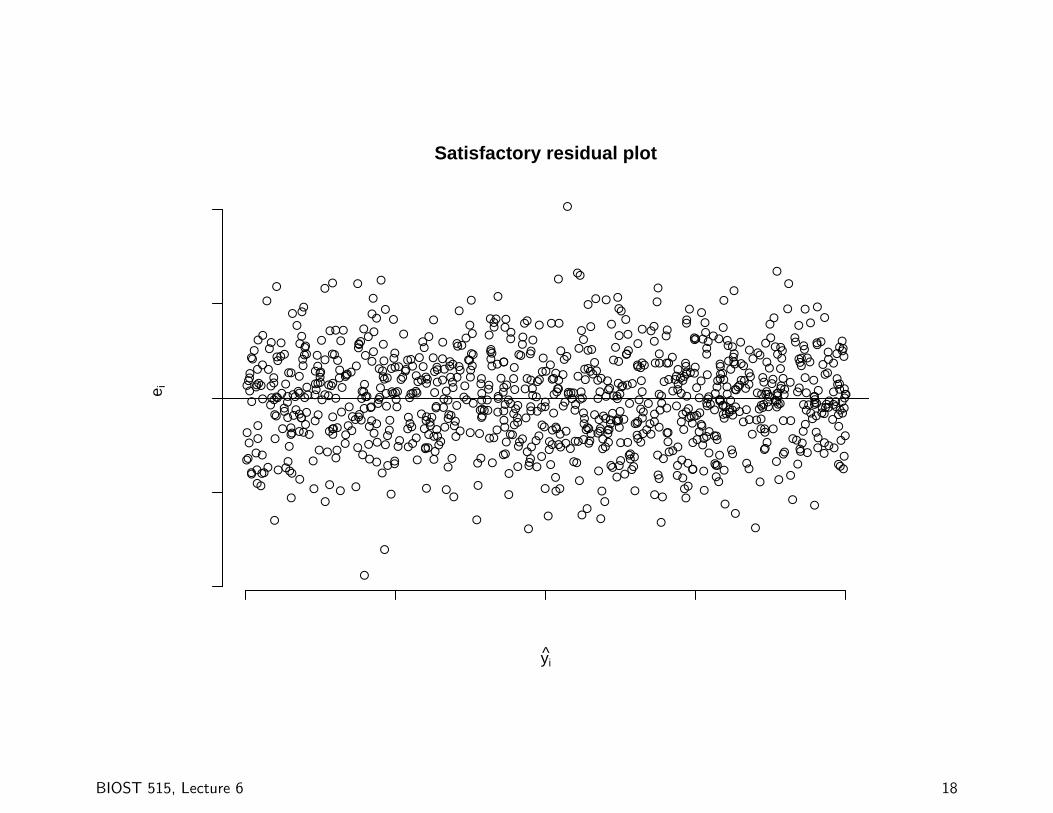
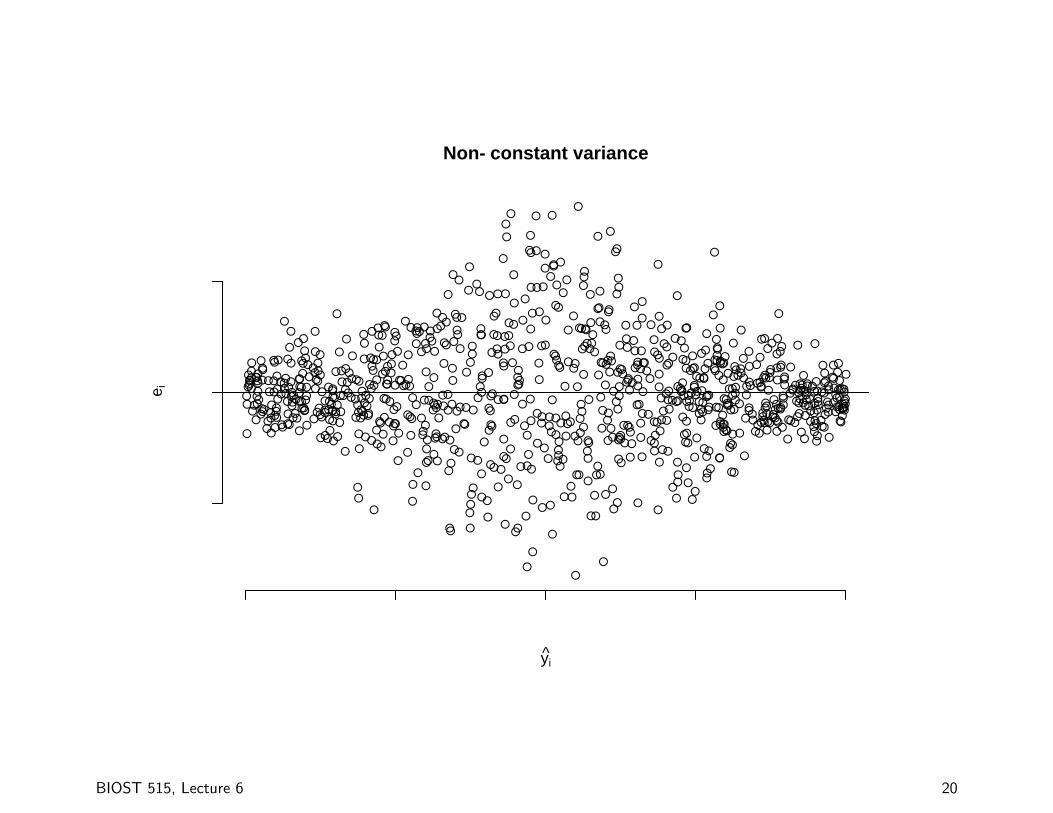
Scatterplots

Another useful aid for inspection is a scatterplot of the

residuals against the fitted values and/or the predictors. These

plots can help us identify:

• Non-constant variance

• Violation of the assumption of linearity

• Potential outliers


●

●

●

●

●

●

●

●

●●

●

●

●●

●

●

●

●

●

●●

●

●●

●

●

●

●

●

●

●

●

●

●

●

●

●

●

●

●

●

●

●

●

●

●●

●

●

●

●

●●

●

●

●

●●

●

●

●

●

●

●

●

●

●

●

●

●

●

●

●

●

●

●●

●

●● ●

●●

●●

●

●●

●●

●

●●

●●

●●

●

●

●

●

●

●

●

● ●

●

●

●

●●

● ●

●

●

●

●

●●

●

●

●

●

●

●

●

●

●

●

●

● ●●

●●

●

●

●

●

●

●

●

●

●

●

●

●●

●

●

●

●

● ●●

●●●

●

●

●

●

●

●

● ●

●

●

●●

●

●

●

●●

●

●

●

●

● ●

●

●●

●●

●

●

●

●

●

●●●

●●

●

● ●●

●

●

●●

●

●●

●

●

●

●

●

●

●

●

●

●

●

●

●

●

●

● ●

●

●

●

●

●

●

●

●

●

●

●

●

●

●●●

● ●●

●

●

●

●●

●

●

●

●

●

●●

●

●

●

●

●

● ●

●

● ●●

●

●●

●

●

●

●

●

●

●

●

●

●

●

●

●

●●

●

●

●

●

●●

●

●

●

●

●

●

●

●

●

●

●

●●●

●

●

●

●

●

●

●

●

●

●

●

●

●

●

●●

●

●●

●

●

●

●

●

●

●

●

●

●

●

●

●

●

●

●

●

●

●

●

●

●

●

●

●

●●

●

●

●

●

●●

●

●

●

●

●

●

●●●

●

●

●

●

●

●

●

●

●

●

●

●

●

●

●

●

●

●

●

●●

●● ●

●●

●

●

●

●

●

● ●

●

●

●

●

●

●

●

●

●

●

●

●

●

●

●

●

●

●

●

●●

●●

●

●

●

●

●

●

●

●

●●

●

●

●

●

●●

●

●

●

●

●

●

●

●

●

●

●

●

●

●

●●

●●

●

●

●

●

●

●

●

● ●

●●

●

●

●

●

●

●

●

●

●

●●

●

●

●

●

●●

●

●

●

●

●

●

●

●

●

●

●●

●

●

●

●

●●

●●

●●

●

●

●●

●

●

●

●

●

●

●

●

● ●●

●●

●

●

●

●

●

●

●

●

●

●

●

●

●

●

●

●

●

●

●

●

●

●

●

●

●

●

●

●

●

●

●

●

●

●

●

●

●

●

●

●

●

●

●

●

●

●

●

●

●

● ●

●

●

●

●

●

●

●

●

●

●

●

●

●

●

●

●

●

●

●

●

●

●

●

●

●

●

●

●

●

●

●

●

●

●●

●

●

●●

●

●

●

●

●

●

●

● ●

●●

●

●●

●

●

●●

●

●● ●

●

●

●

●

●

●

●

●

●●

●

●

●

●

●

●

●

●

●

●

●●

●●

●

●

●

●

●

●●

●●

●

●

●●

●

●

●

●

●●

●

●

●

●

●

●

●

●

●

●

●

●

●●

●

●●

●

●

●

●

●●

●

●

●

●

●

●

●

●

●

●

●

●

●

●

●●

●

●

●

●●

●

● ●

●

●

●

●

●

●

●

●

●

●

●

●

●

●

●

●

●

● ●

●

●

●

●

●

●

●

●

●

●

●

●

●

●

●

● ●● ●

●

●

●●

●

●

●

●

●

●

●

●

●

●

●●

●

●

●●●●

●

●

●

●

●●

●

●

●

●

●

●●

●

●

●

●●

●

●

●

●

●

●

●

●

●

● ●

●

●

●

●●

●

● ●●●

●

●

●

●

●

●

●

●

●

●

●

●

● ●

●

●

●

●

●

●

●

●

●

●

●

●

●

●

●

●

●

●●●

●

●

●

●

●●

● ●

●

●

●

● ●

●

●

●

●

●

●

●

●

●

●

●

●

●

●

●

●

●

●

●●

●

●

●

●

●

●

●

●

●

●

●

● ●

●

●

●

●

●●

●

●

●

●

●

●● ●

●

●

● ●

●●

●

●

●

●

●

●

●

●

●

●

● ●

●

● ●

●

●

●

●

●

●●

●

●

●

●●

●

●

●

●

●

●

●

●●

●

●

●

●

●

●

●

●

●

●●

●

●

●

●

●

●

●

●

●●

●

●

●

●

●

●

●

●

●

●●

●

●

●

●

●

●●

●

●

Satisfactory residual plot

yi

e i


●●

●

●

●

●

●

●

●

●

●●

●

●

●

●

●

●

●

●

●●

●●

●

●

●

●

●

●

●

●

●● ●

●

●

●

●

●

●

●●

●●

●

●

●

●

●

●

●●

●

● ●

●

●

●● ●

● ●

●●

●

●

● ●

●

●

●

●●

●

●

●

●

●

●

●

●

●

●

●

●

●

●●

●

●

●●

●

●●

●

●

●

●

●

●

●

●

● ●

●

●

●

●

●●

●

●

●

●

●

●

●

●●

●

●

●

●

●

●

●● ●

●

●●

●

●

●

●

●●

●

●

●

●

●

●

●

●

●

●

●

●

●●●

●

●

●

●

●

●

●

●

●

●

●

●

●●

●

●

●

●●

●

●●

●

●●

●● ●

●

●

●

●

●

●

●

●●

●

●

●

●

●

● ●●

●

●

●

●

●

●

●

●

●

●

●

●

●

●

●

●

●

●

●

●

●

●

●

●

●

●

●

●

●

●

●

●

●

●●

●

●

●

●

●

●

●

●

●

●

●

●

●

●

● ●●

●

●

●

●

●

●

●

●

●

●

●

●

● ●

●●

●

●

●

●

●

●

●●

●

●

●

●

●● ●

●

●

●

●

●●

● ●●

●

●

●

●

●

●

●

●

●

● ●

●●

●

●

●

●

●

●

●

●

●

●●

●

●

●

●

●

●

●

●

●

●

●

●

●

●

●

●

●

●

●

●

●

●

●

●

●

●

●

●

●

●

●

●

●

● ●

●

●

●

●

●

●●

●

●

●

●

●

●

●

●●

●

●

●

●

●

●

●●

●

●

●●

●

●

●

●

●

●

●

●

●●

●

●●

●

●

●●

●●

● ●

●

●

●

●

●

●

●

●

●

●●

●

●

●

●

●●

●

●

●

●

● ●

●

●

●

●

●

●

●

●●

●

●

●

●

●

●

●

●●

●

●

●

●

●

●

●

●

●

● ●

●

●

●

●

●

●

●●

●

●

●●

●

●

●

●

●

●

●

●●

●

●

●

●

●●

●

●

●

●

●

●

●

● ●●

● ●

●

●

●

●

●

●●

●

●

●

●

●●

●

●

●

●

●

●

●

●

●

●

●

●

●

●

●

●

●

●

●

● ●

●

●

●

●

●

●

●●

●

●

●

●●

●

●

●

●

●●

●

●

●

●

●

●

●

●

●

●

●

●●

●

●

●

●●

●

●

●

●

●

●

●

●

●

●

●

●

●

●●

●

●

●

●

●

●

●

●

●

●

●

●

●●

●

●●

●

●

●

●

●

●

●●

●

●

●

●

●

●

●

●●

●●

● ● ●

●

● ●

●

●

●●

●

●●●

●

●

●

●●

●

●●

●

●

●

●

●

●●

●

●

●●

●

●

●

●

●

●

●

●

●

●

●

●●

●

●

●●●

●

●

●

●

●

●

●

●

● ●

●

●

●

●

●

●

●

●

●

●

●

●●

●

●

●

●

● ●

●

●●

●

●

●

●●

●

●

●

●

●

●

●

●

●●

●

●

●

●

●

●

●

●

●

●

● ●

●

●

●

●

●

●●

●

●

●●

●

●

●

●

●

●

●

●

●

●

● ●

●

●

●●

●

●●

●

●

●

●

●

●

●

●

●

●

●

●

●

●

●

●

●

●

●

● ●

●

●

●

●

●

●

●

●

●

●●

●

●

●

●

●●

● ●

●

●

●

●

●

●

●

●

●

● ●

●

●

●

●

●

●

●

●

●

●

●

●

●

●●●

●

●

●

●●●

●

●

●

●

●

●

●

●

●

●

●

●

●

●

●

●

●●

●

●●

● ●

●

●

●

● ●

●

●●

●

●

●●

●

●

●

●

●

●

●

●

●

●

●

●

●

●

●

●

●

●

●

●

●

●

●

●

●

●

●

●

●●

●●

●

●

●

●

●●

●●

●

●

●●●

●

●

●

●

●

●

●

●

●

●

●●

●

●

●

●

●

●

●

●

●

●

●●

●●

●

●●

●●

●

●

●●

●

●

●

●

●

●

●

●

●

●

●●

●

●

●●

●

●

●●

●

● ●●●

●

●●

●

●

●

●

●

●

●

●

●

●

●

●

●

●

●

● ●

●●

●

●

●

●

●

●

●

●

●

●●

●

●

Non−constant variance

yi

e i


●

●

●

●

●

● ●

●●

●

●

●

●

●

●

●

●

●

●

●

●

●●

●

●

●

●

●

●

●

●

●

●

●

●

●

●

●

●

●

●

●

●●

●

●

●●

●

●

●

●

●

●

●

●

●

●

●

●

●

●●

●

●

●

●

●

●●

●

●

● ●●

●

●

●

●

●

●

●

●

●

●

●

●

●

●

●

●

●

●

●

●

●

●

●

● ●

●

●

●

●

●

●●

●

●

●

●

● ●●

●●

●

●

●

●

●

●

●

●

●

●

●

●

●●

●●

●

●●

●●

●

●

●

●

●

●

●

●●

●

●

●

●

●

●

●

●

●

●●

●

●

●

●

●

●

●

●

●

●

●

●

●

●

●●

●

●

●

●

●

●

●●

●

●

●

●

●

●

●●

● ●

●●

●

●

●

●●

●

●

●

●

●

●

●

●

●●●

●

●

●

●●

●

●●

●●

●

● ●●

● ●

●

●

●●

●

●

●

●

●

●

●

●

●

●

●

●

●

●

●

●

●

●

●

●

●

●

●

●●

●

●

●

●

●

●

●

●

●●

●

●

●

●

●

●

●

●

●

●

●

●

●

●

●●

●

●

●

●

●

●

●

●

●

●

●

●

●

●

●●

● ●

●

●

●

●

●

● ●

●●

●

●● ●

●

●

●

● ●

●

●

●

●

●●

●

●

●

●

●

●

●

●

●

●●

●

●

●

●●

●

●

●

●

●

●

●

●

●

●

●

●

●●

●

●

●

●

●●

●

●

●

●

●

●

●

●

●

●

●

●

●

●

●

●

●

●

●●●

●

●

●

●

●

●

●

●

●

●

●

●

●

●

●

●

●●

●

●

●●

●

●

●

●

●

●

●

●

●

●●

●●

●

●

●

●●

●

●

●

●

●●

●

●●

●●

●

●

●●

●●

●

●

●

●

●●

●

●

●

●

●

●

●● ●

●●

●

●

●

●

●

●

●

●

●

●

●

●

●●

●

●

●

●

●

●

●

●

●

●

●

●

●

●

●

●

●

●

● ●

●

●

●

●

●

●

●

●

●

●

●

●

●

●

●

●

●

●

●

●

●

●

●

●

●●

●

●

●

●

●

●

●

●●●

●

●

●

● ●

●

●●

●●

●

●

●

●●

●

●●

●●

●

●●

●

●

●

●

●●

●

●

●

●

●

●

●●

●

●

●●

●

●

●

●

●

●

●

●●

●

●

●

●

●

●●

●

●

●

●

●

●

●

●

●

●

●

●

●●

●

●

●

●

●

●

● ●

●

●

●

●

●

●

●

●●

●

●

●

●

●

● ●

●

●

●

●

●

●

●● ●●

●

●

●

●

●

●

●

●

●

● ●

●

●

●

●

●

●

●

●

●●●●

●

●

●

●

●

●

●●

●

●

●

●

●

●

●

●

●

●

●

●●

●

●●

●

●

●

●

●

●

●

●

●

●

●

●

●

●●

●●

●●

●

●

● ●

●

●

●

●

●

●●

●

●

●

●●

●

●●●

●

●

● ●●

●

●●

●

●

●

●

●

●

●

●

●

●

●

●

●

●

●

●

●●

●●

●

● ●

●

●

●

●

●

●

●

●

●

●

●●

●

●

●

●

●

●

●

●

●

● ●

●

●●

●

●

●

●●

●

●

●

●

● ●

●

●

●

●

●

●

●

●

●●

●●

●

●

●

●

●

●

●

●

●

●

●

●

●

●

●

●

●

●

●

●

●

●

●

●

●

●

●●

●

●●

●

●

●

●

●

●

●

●

●

●

●

●

●

●

●

●

●

●

●

●

●●

●

●

●

●

●

●

●

●

●

●

●

●

●

●

●

●

●

●

●

●

●

●

●

●

●

●

●●

●

●

●

● ●

●

●

●

●

●

●

●

●

●

●

●

●

●

●

●

●

●

●●

●

●

●

●

●

●

●

●

●

●

●

●

●●

●

●●

●●

●

●

●

●

●

●

●

● ●

●

●

●

●

●

●

●

●●

●

●

●

● ●●

●

●

●

●

●

●

●●

●●

●

●

●

●

●

●

●

●

●

●

●

●

●

●

●

●

●

●

●

●

●

●●

●

●

●

●

●

●

●

●●

●

●

●●

●

●

●

●

●

●

●

●

●

●

●

●

Non−constant variance

yi

e i


Example

Suppose the true relationship between a predictor, x, and

an outcome, y is

E(yi) = 1 + 2xi − 0.25x2i ,

but we fit the model

yi = β0 + β1xi + εi.

Can we diagnose this with residual plots?


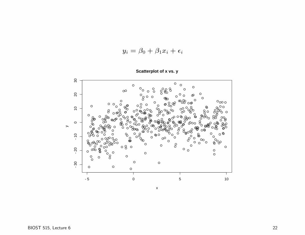
yi = β0 + β1xi + εi

●

●

●

●●

●●

● ●

● ●

●●

●

●

●

●●

●

●

●

●

●

●

●

●

●

●

●

●

●

●

●

●

●

●

●

●

●

●●●

●

●

●

●

●

●●

●

●

●

●

●

●●

●

●

●

●

●

●

●

●

●

●

● ●

●

●

●

●

●●

●

●

●

●

●

●

●

●

●

●●

●

●

●

●

●

●

●

●

●

●

●●

●

●

●

●

●

●

●

●

●

●

●

●

●

●

●

●●

●

●

●

●

●

●

●

●

●

●

●

●

●

●

●

●

●

●

●

●

●● ●

●

●

●

●

●

●

●

●

●

●

●

●

●

●

●

●

●

●

●

●

●

●

●

●

●

●

●

●

●

●●

●

●

●

●

●

●

●

●

●●

●

●

●

●

●

●

●

●●●

●● ●●

●

●

●●

●

●

●

●

●

●

●

●

●

●

●●

●

●

●

●

●

●

●

●

●

●

●

●

●

●

●

●

●

●

●

●

●

●

●

●

●

●● ●

●

●

● ●

● ●●

●

●

●

●

●●

●

●

●

●

●

●

●

●

●

●

●

●

●

●

●

●●

●

●

●

●●

● ●

●

●

●

●

●

●

●

●

●

●

● ●

●

●

●

● ●

●

●

●

●

●

●

●

●

●

●

●

●

●

●

●

●

●

●

●

●

● ●

●

●

●●

●

●●

●

●

●

●

●

●

●

●

●

●

●

●

●

●

●

●●

●●

●

●

●

●

● ●

●

●

●

●

●

●

●

●

●

●

●

●

●

●

●

●

●

●

●

●

●

●

●

●

●

● ●

●

●●

●

●

●

●●

●

●

●

●

●

●

●

●

●

●

●

●

●●

●

●

●

●●

●

●

●

●

●

●

●

●

●

●

●

●

●

●

●

●●

●

●

●

●

●

●

●

●

●

●

●

●

●

●

●

●

●

●

●

●

●

●

●

●

●

●

●

●

●

●

●

●

●

●

●

●

●

●

●

●

●

●●

●

●

●

●

●●

●●

●

●

●

●

●

●

●

●

●● ●

●

●

●

●

●

●

●

●

●

●●●

●

●

●

●

●

●

●

●

●

●

●

−5 0 5 10

−30

−20

−10

010

2030

Scatterplot of x vs. y

x

y


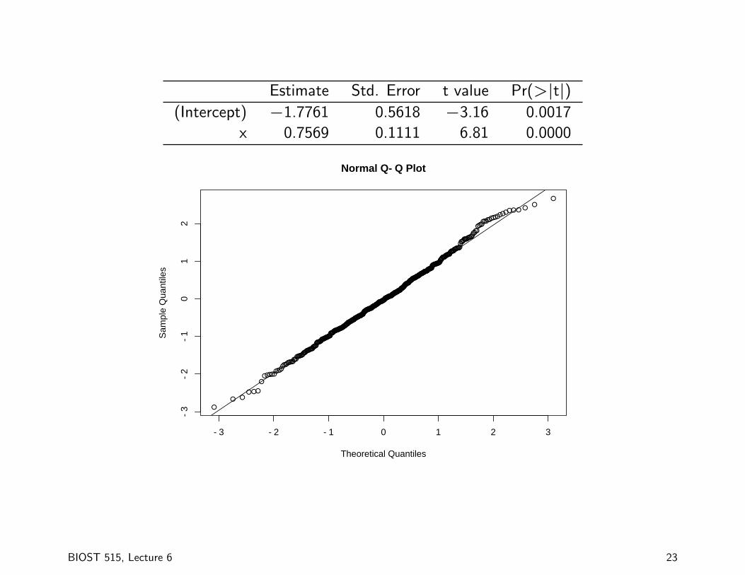
Estimate Std. Error t value Pr(>|t|)(Intercept) −1.7761 0.5618 −3.16 0.0017

x 0.7569 0.1111 6.81 0.0000

●

●

●

●

●

●●

●

●

●●

●

●

●

●

●

●

●

●

●

●

●●

●

●

●

●

●

●

●

●

●

●

●

●

●

●

●

●

●

●

●

●

●

●

●

●

●

●

●

●

●

●

●

●

●

●

●

●●

●

●

●

●

●

●

●

●

●

●

●

●●

●

●

●

●

●

●

●

●

●

●

●

●

●

●

●

●

●

●

●

●

●

●

●

●

● ●

●●

●

●

●

●

●

●●

●

●

●

●

●

●

●

●

●

●

●

●

●

●

●●

●

●

●

●

●

●●

●

●

●

●

●

●

●

●

●

●

●

●

●

●

●●

●

●

●

●

●

●

●

●

●

●

●

●

●

●

●

●

●

●

●

●●

●

●

●

●

●

●

●

●

●

●

●

●

●

●

●

●

●

●●

●

●

●

●

●

●

●

●●

●

●

●

●

●

●

●

●

●

●

●●

●

●●

●

●

●

●

●

●

●

●

●

●●

●●

●

●

●

● ●

●

●

●

●

●

●

●●

●

●

●●

●●

●

●●

●

●●

●

●

●

●●

●

●

●

●

●

●

●

●

●

●

●

●

●

●●

●●

●●

●

●

●

●

●

●

●

●

●

●

●●

●

●

●

●

●

●

●

●

●

●●

●

●

●

●

●

●

●

●

●●

●

●

●

●

●

●

●

●

●

●

●

●

●

●

●

●●

●●

●

●

●

●

●

●

●

●

●

●

●

●

●

●●

●

●

●

●

●

●

●

●

●

●

●

●

●

●

●

●

●

●

●

●

●

●

●●

●

●

●

●

●

●

●

●

●

●

●

●

●

●●

●

●

●

●

●

●

●

●

●

●

●

●

●

●

●

●

●

●

●

●

●●

●

●

●

●

●

●●

●

●

●

●

●

●●

●

●

●

●

●

●

●

●

●

●

●

●

●

●

●

●●

●

●

●

●●

●

●

●

●

●

●

●

●

●●

●

●

●●

●

●

●

●

●●

●

●

●

●

●

●

●

●

●

●

●

●

●

●●

●

●

●●

●

●

●

●

●

●

●

●

●

●

●●●

●

●

●●

●

●

●

●

●

●

●

−3 −2 −1 0 1 2 3

−3

−2

−1

01

2

Normal Q−Q Plot


Sam

ple

Qua

ntile

s


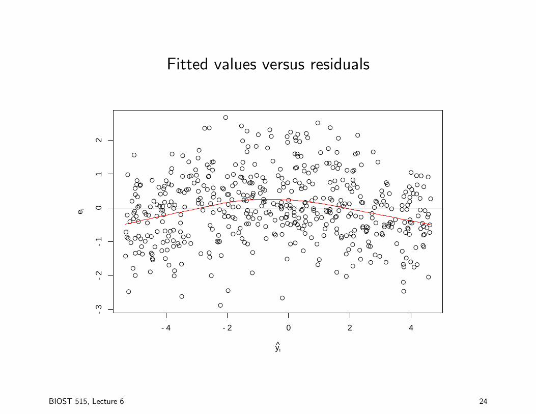
Fitted values versus residuals

●

●

●

●

●

●●

●

●

● ●

●

●

●

●

●

●

●

●

●

●

●●

●

●

●

●

●

●

●

●

●

●

●

●

●

●

●

●

●

●

●

●

●

●

●

●

●

●

●

●

●

●

●

●

●

●

●

●●

●

●

●

●

●

●

●

●

●

●

●

●●

●

●

●

●

●

●

●

●

●

●

●

●

●

●

●

●

●

●

●

●

●

●

●

●

● ●

● ●

●

●

●

●

●

●●

●

●

●

●

●

●

●

●

●

●

●

●

●

●

●●

●

●

●

●

●

●●

●

●

●

●

●

●

●

●

●

●

●

●

●

●

●●

●

●

●

●

●

●

●

●

●

●

●

●

●

●

●

●

●

●

●

●●

●

●

●

●

●

●

●

●

●

●

●

●

●

●

●

●

●

●●

●

●

●

●

●

●

●

●●

●

●

●

●

●

●

●

●

●

●

●●

●

●●

●

●

●

●

●

●

●

●

●

● ●

● ●

●

●

●

●●

●

●

●

●

●

●

●●

●

●

●●

●●

●

●●

●

●●

●

●

●

●●

●

●

●

●

●

●

●

●

●

●

●

●

●

●●

●●

●●

●

●

●

●

●

●

●

●

●

●

●●

●

●

●

●

●

●

●

●

●

●●

●

●

●

●

●

●

●

●

●●

●

●

●

●

●

●

●

●

●

●

●

●

●

●

●

● ●

●●

●

●

●

●

●

●

●

●

●

●

●

●

●

●●

●

●

●

●

●

●

●

●

●

●

●

●

●

●

●

●

●

●

●

●

●

●

●●

●

●

●

●

●

●

●

●

●

●

●

●

●

●●

●

●

●

●

●

●

●

●

●

●

●

●

●

●

●

●

●

●

●

●

●●

●

●

●

●

●

●●

●

●

●

●

●

●●

●

●

●

●

●

●

●

●

●

●

●

●

●

●

●

●●

●

●

●

●●

●

●

●

●

●

●

●

●

● ●

●

●

●●

●

●

●

●

● ●

●

●

●

●

●

●

●

●

●

●

●

●

●

●●

●

●

●●

●

●

●

●

●

●

●

●

●

●

●●●

●

●

●●

●

●

●

●

●

●

●

−4 −2 0 2 4

−3

−2

−1

01

2

yi

e i


Next, we fit

yi = β0 + β1xi + β2x2i + εi.

Estimate Std. Error t value Pr(>|t|)(Intercept) 1.9824 0.6000 3.30 0.0010

x 1.9653 0.1637 12.00 0.0000

x2 −0.2640 0.0268 −9.85 0.0000

●

●

●●

●

●

●

●

●

●●

●

●

●

●

●

●●

●

●●

●

●

●

●

●

●

●

●

●

●

●

●

●

●

●

●

●●●

●

●

●

●

●●

●

●●●

●

●

●

●

●

●

●

●

●

●●

●

●

●

●

●

●●

●

●

●

●

●●

●

●

●

●

●

●

●

●

●

●

●

●

●

●

●

●

●

●●

●

●

●

●

●●

●●

●

●

●

●●

●

●

●

●

●

●

●

●●

●

●

●

●

●

●

●

●●

●

●

●

●

●

●

●●

●

●

●

●

●

●

●

●

●

●

●

●

●

●

●

●

●

●

●

●

●

●

●●

●

●

●

●

●

●

●

●

●

●

●

●

●

●

●

●

●

●

●

●

●●

●

●

●

●

●

●

●

●

●

●

●

●

●

●

●

●

●

●

●

●

●

●

●

●●

●

●

●

●

●

●

●

●

●

●●

●

●

●

●

●●

●

●

●●

●

●

●

●●

●●

●●●

●

●

●●●

●

●

●●

●

●●

●●

●

●

●

●

●

●

●

●

●

●

●

●

●

●

●

●

●

●

●

●●

●●

●●

●

●

●

●

●

●

●

●

●

●

●●

●

●

●

●

●

●

●

●

●

●

●

●

●

●

●●

●

●

●

●

●●

●

●

●

●

●

●

●

●

●

●

●

●

●

●

●

●

●

●

●

●

●

●

●

●

●

●

●

●

●

●

●

●

●

●

●

●

●

●

●

●

●

●

●

●

●

●

●●

●

●

●

●

●

●

●

●●●

●

●

●

●

●

●

●

●

●

●

●

●

●

●●

●

●

●●

●●●

●

●

●

●

●●

●

●

●

●

●

●

●

●

●

●

●

●

●

●

●

●

●

●

●

●

●

●

●

●

●

●

●

●●●

●

●

●

●

●

●

●

●

●

●

●

●

●

●

●

●

●

●

●

●

●

●

●

●

●

●

●

●

●

●

●

●

●

●

●

●

●●

●

●

●

●

●

●

●

●

●

●

●

●

●

●

●

●

●

●

●

●

●

●

●

●

●

●

●

●●

●

●

●

●

●

●

●

●

●

●

−3 −2 −1 0 1 2 3

−3

−2

−1

01

2

Normal Q−Q Plot


Sam

ple

Qua

ntile

s


Fitted values versus residuals

●

●

●●

●

●

●

●

●

● ●

●

●

●

●

●

●●

●

●●

●

●

●

●

●

●

●

●

●

●

●

●

●

●

●

●

● ●●

●

●

●

●

●●

●

●●●

●

●

●

●

●

●

●

●

●

●●

●

●

●

●

●

●●

●

●

●

●

●●

●

●

●

●

●

●

●

●

●

●

●

●

●

●

●

●

●

●●

●

●

●

●

●●

●●

●

●

●

●●

●

●

●

●

●

●

●

● ●

●

●

●

●

●

●

●

●●

●

●

●

●

●

●

●●

●

●

●

●

●

●

●

●

●

●

●

●

●

●

●

●

●

●

●

●

●

●

●●

●

●

●

●

●

●

●

●

●

●

●

●

●

●

●

●

●

●

●

●

● ●

●

●

●

●

●

●

●

●

●

●

●

●

●

●

●

●

●

●

●

●

●

●

●

●●

●

●

●

●

●

●

●

●

●

● ●

●

●

●

●

●●

●

●

●●

●

●

●

●●

●●

● ●●

●

●

●● ●

●

●

●●

●

●●

●●

●

●

●

●

●

●

●

●

●

●

●

●

●

●

●

●

●

●

●

●●

● ●

●●

●

●

●

●

●

●

●

●

●

●

●●

●

●

●

●

●

●

●

●

●

●

●

●

●

●

●●

●

●

●

●

●●

●

●

●

●

●

●

●

●

●

●

●

●

●

●

●

●

●

●

●

●

●

●

●

●

●

●

●

●

●

●

●

●

●

●

●

●

●

●

●

●

●

●

●

●

●

●

●●

●

●

●

●

●

●

●

●● ●

●

●

●

●

●

●

●

●

●

●

●

●

●

●●

●

●

● ●

●●●

●

●

●

●

● ●

●

●

●

●

●

●

●

●

●

●

●

●

●

●

●

●

●

●

●

●

●

●

●

●

●

●

●

●● ●

●

●

●

●

●

●

●

●

●

●

●

●

●

●

●

●

●

●

●

●

●

●

●

●

●

●

●

●

●

●

●

●

●

●

●

●

●●

●

●

●

●

●

●

●

●

●

●

●

●

●

●

●

●

●

●

●

●

●

●

●

●

●

●

●

●●

●

●

●

●

●

●

●

●

●

●

−10 −5 0

−3

−2

−1

01

2

yi

e i


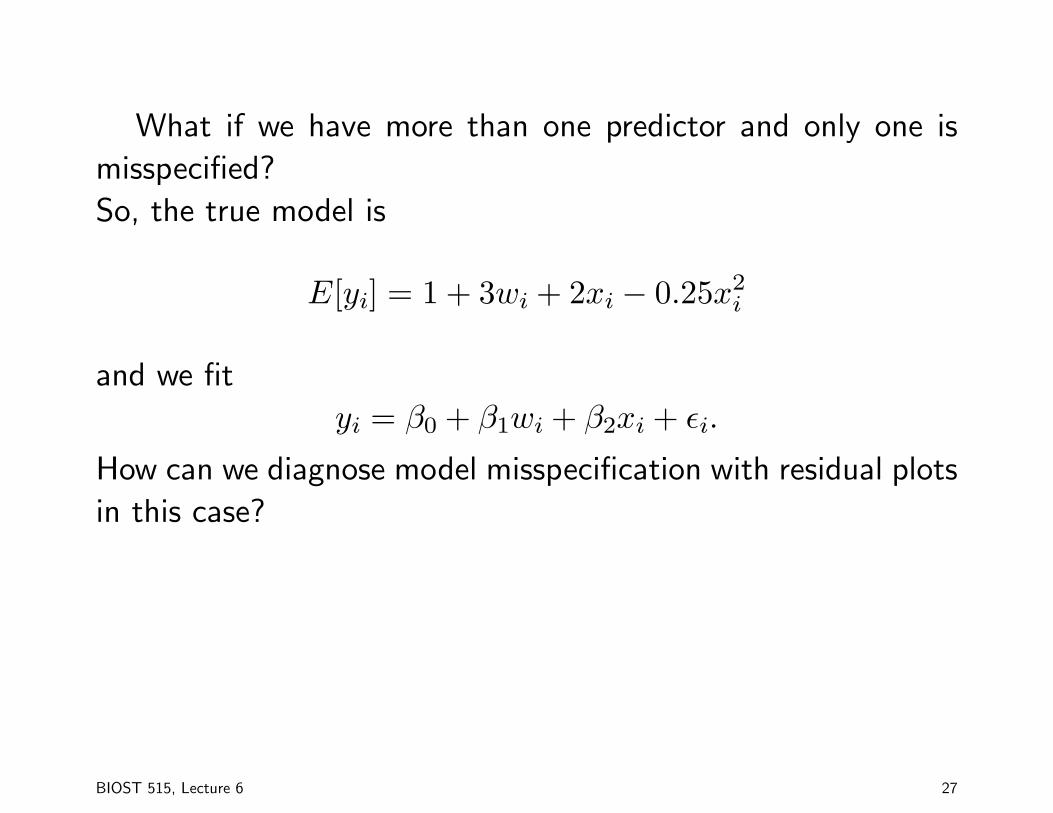
What if we have more than one predictor and only one is

misspecified?

So, the true model is

E[yi] = 1 + 3wi + 2xi − 0.25x2i

and we fit

yi = β0 + β1wi + β2xi + εi.

How can we diagnose model misspecification with residual plots

in this case?


y

2.0 2.5 3.0 3.5 4.0

●●

●

●●

●

●

● ●

●

●

●●

● ●

●●

●

●

●

●

●

●

●

●

●

●●

●

●

●

●

●

●

●●

●

●●

●

●

●

●

●

●

●

●

●●

● ●●●

●

●

●

●

●

●

●

●●

●

●

●

●

●

●

●

●

●

●

●

●●

●

●

●

●

●

●

●

● ●●●

●

●

●

●

●

●

●

●●

● ●

●●

●

●●

●

●

●

●

●●

●

●

●

●

●

●●

●

●●

●●

●

●● ●

●

●

●

●●●

●

● ●

●

●●

●

●●

●

●●

●

●

●

●●

●

●

● ●

●

●

●

● ●

●

●

●

●●

●

●

●

● ●

●

●

●

●●

●

●●

●

●

●

●●

●

●●

●

●

●

●

●

●

●

●

●●

●

●

●●

●●●

●

●

●

●

●

●

●●

●

●

●

●

●

●●

●

●

●●

●

●

●

●

●

●

●

●

●

●

●

●

●

●

●

●

●●

●●

●

●●

●

●

●

●

●

●

●

●

●

●

●

●

●

●

●

●●

●

●

●

●

●

●●

●

●●

●

● ●

●

●

●

●

●

●●

●

●●

●

●

●

●●

●

●

●

●

●

● ●

●

●

●

●

●

● ●

●

●

●●

●

●

●

●

●

● ●

●

●

●

●

●

●

●

●

●

●

●

●

●

●●

●

●

● ●

●

●

●

●

●●

●

●

●

●

●

●●

●

●

●

●

●

●●

●

●●

●

●

●

●

●●

●

●

● ●●

●

●

●●

●●

●

●

●

●

●

●

●

●●

●

●

●

●●

● ●

●

●

●

●

●●

●

●

● ●

●●●

●●

●

●

●

●

●

●

●

●

●

●

●

●

●

●

●

●

●

●

●●

●

●

● ●●

●

●

●

●

●

●

●

●●

●

● ●●

●

●●●

●

●●

●

●

●

●●

●

●

●

●●

●

●

●●

●●

● ●

●

●

●

●

●●

●●

●

●●●●

●

●

●

●

●

●

●

● ●

●●

●

●

●

●

●

●

●

●

●

●

●

●

−20

020

40

●●

●

●●

●

●

●●

●

●

●●

● ●

●●

●

●

●

●

●

●

●

●

●

●●

●

●

●

●

●

●

●●

●

●●

●

●

●

●

●

●

●

●

●●

●● ●●

●

●

●

●

●

●

●

●●

●

●

●

●

●

●

●

●

●

●

●

●●

●

●

●

●

●

●

●

●●●●

●

●

●

●

●

●

●

●●

● ●

●●

●

●●

●

●

●

●

●●

●

●

●

●

●

●●

●

●●

●●

●

●● ●

●

●

●

●●●

●

●●

●

●●

●

●●

●

●●

●

●

●

●●

●

●

● ●

●

●

●

●●

●

●

●

● ●

●

●

●

● ●

●

●

●

●●

●

●●

●

●

●

●●

●

●●

●

●

●

●

●

●

●

●

●●

●

●

●●

●●●

●

●

●

●

●

●

●●

●

●

●

●

●

●●

●

●

●●

●

●

●

●

●

●

●

●

●

●

●

●

●

●

●

●

●●

● ●

●

●●

●

●

●

●

●

●

●

●

●

●

●

●

●

●

●

●●

●

●

●

●

●

●●

●

●●

●

● ●

●

●

●

●

●

●●

●

●●

●

●

●

●●

●

●

●

●

●

●●

●

●

●

●

●

● ●

●

●

●●

●

●

●

●

●

●●

●

●

●

●

●

●

●

●

●

●

●

●

●

●●

●

●

●●

●

●

●

●

●●

●

●

●

●

●

●●

●

●

●

●

●

●●

●

●●

●

●

●

●

●●

●

●

● ●●

●

●

●●

●●

●

●

●

●

●

●

●

●●

●

●

●

●●

● ●

●

●

●

●

●●

●

●

● ●

●●●

● ●

●

●

●

●

●

●

●

●

●

●

●

●

●

●

●

●

●

●

●●

●

●

● ●●

●

●

●

●

●

●

●

●●

●

● ●●

●

●●●

●

●●

●

●

●

● ●

●

●

●

●●

●

●

●●

●●

● ●

●

●

●

●

●●

●●

●

●●●●

●

●

●

●

●

●

●

● ●

●●

●

●

●

●

●

●

●

●

●

●

●

●

2.0

2.5

3.0

3.5

4.0

●

●

●

●

●

●

●

●●

●

●

●

●

●●

●

●●

●

●

●

●

●●

●

●

●

●

●

●

●

●

●

●

●

●

●

●

●●

●

●

●

●

●

●

●

●

●

●

●●

●

● ●

●

●

●

●●

●

●●

●

●

●●

●

●

●

●

●●

●

●

●●

●

●

●

●●

●

●

●

●

●

●

●

●

●

●

●

● ●

●

●

●●

●

●

●

●

●

●

●●

●

●

●

●

●

●

●

●

●

●

●

●

●●

●

●

●

●

●

●

●

●

●

●

●

●

●●

●

●

●

●●

●

●

●

●

●

●

●●

●●

●

●

●

●

●

●●

●

●

●

●

●

●

●

●

●

●●

●

●

●

●

●

●

●

●

●

●

●

●

●●

●

●

●●

●

●

●

●

●

●

●

●

●

●

●

●

●

●

●

●

●

●

●

●

●

●

●

●

●

●

●

●

●

●

●

●

●

●

●●

●

●

●

●

●

●

●

●

●● ●

●

●

●

●●

●

●●●

●

●

●

●

●

● ●

●

●

●

●

●

●

●●

●

●

●●

●

●●

●●

●●

●

●

●●

●●

●

●

●

●

●

●

●

●

●

●

●●

●

●●

●

●●

●

●

●

●

●

●●

●

●●

●

●

●

●

●

●

●

●

●

●

●

●

●

●

●

●● ●

●

●

●

●

●●

●

●

●

●

●

●

●

●

●

●●

●

●

●●●

●

●

●

●

●

●

●●

●

●

●

●

●

●

●

●

●

● ●

●

●

●

● ●

● ●●

●

●

●

●

●

●

●

●

●

●

●

●

●

●

●

●

●

●

●●

●

●

●

●

●

●

● ●

●

●

●

●

●

●●

●

●

●●

●

●

●

●

●

●

●

●

●

●

●

●●

●●

●

●

●

●

●

●

●

●

●

●

●

●●

●

●

●

●

●

●

●

●

●

●

●

●

●

●

●

●

●

●

●

●

●

●

●

●

●

●

●

●

●

●

●

●

●

●

●

●

●

●

●

●

●

●

● ●

●

●

●

●

●

●

●

●

●

●

● ●

●●

●●

●

●

●

●

w●

●

●

●

●

●

●

●●

●

●

●

●

●●

●

●●

●

●

●

●

●●

●

●

●

●

●

●

●

●

●

●

●

●

●

●

●●

●

●

●

●

●

●

●

●

●

●

● ●

●

● ●

●

●

●

●●

●

●●

●

●

●●

●

●

●

●

●●

●

●

●●

●

●

●

●●

●

●

●

●

●

●

●

●

●

●

●

● ●

●

●

●●

●

●

●

●

●

●

●●

●

●

●

●

●

●

●

●

●

●

●

●

●●

●

●

●

●

●

●

●

●

●

●

●

●

●●

●

●

●

●●

●

●

●

●

●

●

●●

●●

●

●

●

●

●

●●

●

●

●

●

●

●

●

●

●

●●

●

●

●

●

●

●

●

●

●

●

●

●

●●

●

●

●●

●

●

●

●

●

●

●

●

●

●

●

●

●

●

●

●

●

●

●

●

●

●

●

●

●

●

●

●

●

●

●

●

●

●

●●

●

●

●

●

●

●

●

●

●●●

●

●

●

● ●

●

●●●

●

●

●

●

●

● ●

●

●

●

●

●

●

●●

●

●

●●

●

●●

●●

●●

●

●

●●

●●

●

●

●

●

●

●

●

●

●

●

●●

●

●●

●

●●

●

●

●

●

●

●●

●

●●

●

●

●

●

●

●

●

●

●

●

●

●

●

●

●

●● ●

●

●

●

●

●●

●

●

●

●

●

●

●

●

●

●●

●

●

●● ●

●

●

●

●

●

●

●●

●

●

●

●

●

●

●

●

●

●●

●

●

●

●●

● ●●

●

●

●

●

●

●

●

●

●

●

●

●

●

●

●

●

●

●

●●

●

●

●

●

●

●

● ●

●

●

●

●

●

●●

●

●

●●

●

●

●

●

●

●

●

●

●

●

●

●●

●●

●

●

●

●

●

●

●

●

●

●

●

●●

●

●

●

●

●

●

●

●

●

●

●

●

●

●

●

●

●

●

●

●

●

●

●

●

●

●

●

●

●

●

●

●

●

●

●

●

●

●

●

●

●

●

● ●

●

●

●

●

●

●

●

●

●

●

● ●

●●

●●

●

●

●

●

−20 0 20 40

●

●

●

●

●

●

●

●

●

●

●●

●●

●

●

●

●

●●

●

●

●

●

●

●

● ●

●

●

●

●

●

●

●

●

●●

●

●

●

●

●

●

●

● ●

●

●

●

●

●

●

●

●

●

●

●

●

●

●

●

●

●

●

●●

●

●

●

●

●

●

●

●

●

●

●

●●

●

●●

●

●●

●

● ●●

●

●

●

●●

●

●

●

●

●

●

●

●

●

●

●

●

●

●

●

●

●●

●

●

●

●

●

●●

●●

●

●●●

●

●

●● ●

●

● ●

●

●

●

●

● ●

●

●

●

●●

●

●

●

●

●

●●

●

●

●●

●

●

●

●

●

●

●

●

●

●

●

●●

●

●

●

●

●

●

●

●

●

●

●●

●

●●

●

●●

●

●

●

●

●

●

●

●●

●

●

●

●

●

●

●

●

●

●

●

●

●

●

●

●

●

●

●●

●

●

●

●

●

● ●

●

●

●

●

●●

●

●

●

●

●

●

●

●

●

●

●

●

●

●

●

●

●

●

●

●

●

●

●

●

●

●

●

●

●

●

●●

●●

●

●

●

●

●

●

●

●

●

●

●

●

●

●

●

●

●

●

●

●

●

●

●

●

●

●

●

●●

●

●

●

●

●

●

●

●

●

●

●

●

●

●

●

●

●

●

●

●

●

●

●

●●

●

●

●

●●

●●

●

●

●●

●

●

●

●

●

●

●

●

●

●

●

●

●

●

●

●

●

●

●

●

●

●

●

●

●

●

●●

●

●

●

● ●

●

●

●

●

●

●

● ●

● ●

●

●

●

●

●

●

●

●

●

●

●

●

●

●

●

●

●

●

●

●

●

●

●

●

●

●

●

●

●

●

●

●

●

●

●

●

●

●●

●●

●

●

●

●

●

●

●

●

●

●

●

●

●●

●●

●

●

●

●

●

●

●●

●

●

●

●

●

●

●

●

●

●

●

●

●

●

●

●●

●

●

●

●

●

●

●

●

●

●

●

●

●

●

●

●

●

●

●●

●●

●

●

●

●

●

●

●

●

●

●

●

●

●

●

●●

●

●

●

●

●

●

●

●●

●

●

●

●

●

●

●

●

●

●

●●

●●

●

●

●

●

●●

●

●

●

●

●

●

● ●

●

●

●

●

●

●

●

●

●●

●

●

●

●

●

●

●

● ●

●

●

●

●

●

●

●

●

●

●

●

●

●

●

●

●

●

●

●●

●

●

●

●

●

●

●

●

●

●

●

●●

●

●●

●

●●

●

● ●●

●

●

●

●●

●

●

●

●

●

●

●

●

●

●

●

●

●

●

●

●

●●

●

●

●

●

●

●●

●●

●

●●●

●

●

●● ●

●

● ●

●

●

●

●

●●

●

●

●

●●

●

●

●

●

●

●●

●

●

●●

●

●

●

●

●

●

●

●

●

●

●

●●

●

●

●

●

●

●

●

●

●

●

●●

●

●●

●

●●

●

●

●

●

●

●

●

●●

●

●

●

●

●

●

●

●

●

●

●

●

●

●

●

●

●

●

●●

●

●

●

●

●

● ●

●

●

●

●

● ●

●

●

●

●

●

●

●

●

●

●

●

●

●

●

●

●

●

●

●

●

●

●

●

●

●

●

●

●

●

●

●●

●●

●

●

●

●

●

●

●

●

●

●

●

●

●

●

●

●

●

●

●

●

●

●

●

●

●

●

●

●●

●

●

●

●

●

●

●

●

●

●

●

●

●

●

●

●

●

●

●

●

●

●

●

●●

●

●

●

●●

●●

●

●

●●

●

●

●

●

●

●

●

●

●

●

●

●

●

●

●

●

●

●

●

●

●

●

●

●

●

●

●●

●

●

●

●●

●

●

●

●

●

●

● ●

● ●

●

●

●

●

●

●

●

●

●

●

●

●

●

●

●

●

●

●

●

●

●

●

●

●

●

●

●

●

●

●

●

●

●

●

●

●

●

●●

●●

●

●

●

●

●

●

●

●

●

●

●

●

●●

●●

●

●

●

●

●

●

●●

●

●

●

●

●

●

●

●

●

●

●

●

●

●

●

●●

●

●

●

●

●

●

●

●

●

●

●

●

●

●

●

●

●

●

●●

●●

●

●

●

●

●

●

●

●

●

●

●

●

●

●

●●

●

●

●

●

●

●

●

● ●

−5 0 5 10

−5

05

10

x



x 1.1326 0.1137 9.96 0.0000

w 2.9216 0.8532 3.42 0.0007

●

●

●

●

●

●

●

●

●

●

●

●●

●

●

●

●

●

●

●

●

●

●

●● ●

●●●

●

●

●

●

●

●

●

●

●●

●

●

●

●

●

●

●

●

●●●

●

●

●

●

●

●

●

●

●

●

●

●

●

●

●

●

●

●

●

●

●

●

●

●

●

●

●

●

●

●

●

●

●●

●●

●

●

●

●

●

●

●

●

●

●

●

●

●

●

●

●

●

●

●

●

●

●

●

●

●

●

●

●

●

●

●●

●

●

●

●●

●

●

●

●

●

●●

●

●

●

●●

●

●

●

●

●●

●

●

●

●

●●

●

●

●●

●

●

●

●●

●

●

●

●

●

●

●

●

●

●

●

●

●

●

●

●

●

●

●

●

●

●

●

●

●●

●

●●

●

●

●

●●

●●

●

●

●●

●

●●

●●

●

●

●

●

●●

●

●

●

●●

●

●●

●

●

●●

●

●

●

●

●

●

●

●

●

●

●

●

●

●

●

●

●

●

●

●

●●

●

●

●

●

●

●

●

●●

●

●●

●

●

●

●●●

●

●

●

●

●

●

●

●

●●

●

●

●●

●

●

●

●

●

●

●

●

●

●

●

●●

●

●

●

●

●

●●

●

●

●

●

●

●

●

●

●

●

●●

●

●

●

●

●●

●

●

●

●

●

●

●

●

●

●

●

●

●

●

●

●

●

●●

●

●●

●

●●

●

●

●

●

●

●●

●

●

●

●

●

●

●

●

●

●

●

●

●

●

●

●

●

●

●

●

●

●

●

●●

●●

●

●

●

●

●

●

●●

●

●

●

●● ●

●

●

●

●

●

●

●

●

●●

●

●

●

●

●

●●●●

●

●

●

●

●

●

●

●

●

●

●●

●

●

●

●

●●

●

●

●

●●

●

●

●

●

●

●

●

●

●

●

●●

●

●

●

●

●

●

●

●

●

●

●

●

●

●

●

●

●

●

●

●●●

●

●

●

●

●

●

●

●

●●

●●

●

●●

●

●

●

●

●

●

●

●

●

●

●

●

●

●●

●

●

●

●

●

●

●

●

●

●

−3 −2 −1 0 1 2 3

−4

−3

−2

−1

01

23

Normal Q−Q Plot


Sam

ple

Qua

ntile

s


●

●

●

●

●

●

●

●

●

●

●

●●

●

●

●

●

●

●

●

●

●

●

●● ●

●●●

●

●

●

●

●

●

●

●

●●

●

●

●

●

●

●

●

●

● ●●

●

●

●

●

●

●

●

●

●

●

●

●

●

●

●

●

●

●

●

●

●

●

●

●

●

●

●

●

●

●

●

●

● ●

●●

●

●

●

●

●

●

●

●

●

●

●

●

●

●

●

●

●

●

●

●

●

●

●

●

●

●

●

●

●

●

●●

●

●

●

●●

●

●

●

●

●

●●

●

●

●

●●

●

●

●

●

●●

●

●

●

●

●●

●

●

●●

●

●

●

●●

●

●

●

●

●

●

●

●

●

●

●

●

●

●

●

●

●

●

●

●

●

●

●

●

●●

●

●●

●

●

●

●●

●●

●

●

●●

●

●●

●●

●

●

●

●

●●

●

●

●

● ●

●

●●

●

●

●●

●

●

●

●

●

●

●

●

●

●

●

●

●

●

●

●

●

●

●

●

●●

●

●

●

●

●

●

●

●●

●

●●

●

●

●

●●●

●

●

●

●

●

●

●

●

●●

●

●

●●

●

●

●

●

●

●

●

●

●

●

●

●●

●

●

●

●

●

●●

●

●

●

●

●

●

●

●

●

●

●●

●

●

●

●

●●

●

●

●

●

●

●

●

●

●

●

●

●

●

●

●

●

●

●●

●

●●

●

●●

●

●

●

●

●

●●

●

●

●

●

●

●

●

●

●

●

●

●

●

●

●

●

●

●

●

●

●

●

●

●●

●●

●

●

●

●

●

●

●●

●

●

●

●● ●

●

●

●

●

●

●

●

●

●●

●

●

●

●

●

●●●●

●

●

●

●

●

●

●

●

●

●

●●

●

●

●

●

●●

●

●

●

● ●

●

●

●

●

●

●

●

●

●

●

●●

●

●

●

●

●

●

●

●

●

●

●

●

●

●

●

●

●

●

●

●● ●

●

●

●

●

●

●

●

●

●●

●●

●

●●

●

●

●

●

●

●

●

●

●

●

●

●

●

●●

●

●

●

●

●

●

●

●

●

●

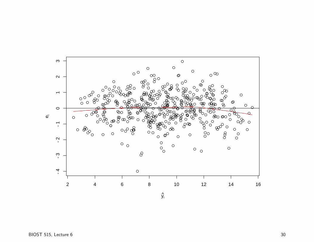
2 4 6 8 10 12 14 16

−4

−3

−2

−1

01

23

yi

e i


●

●

●

●

●

●

●

●

●

●

●

●●

●

●

●

●

●

●

●

●

●

●

●●●

●●●

●

●

●

●

●

●

●

●

●●

●

●

●

●

●

●

●

●

● ●●

●

●

●

●

●

●

●

●

●

●

●

●

●

●

●

●

●

●

●

●

●

●

●

●

●

●

●

●

●

●

●

●

●●

●●

●

●

●

●

●

●

●

●

●

●

●

●

●

●

●

●

●

●

●

●

●

●

●

●

●

●

●

●

●

●

●●

●

●

●

●●

●

●

●

●

●

●●

●

●

●

●●

●

●

●

●

●●

●

●

●

●

●●

●

●

●●

●

●

●

●●

●

●

●

●

●

●

●

●

●

●

●

●

●

●

●

●

●

●

●

●

●

●

●

●

●●

●

●●

●

●

●

●●

●●

●

●

●●

●

●●

●●

●

●

●

●

●●

●

●

●

● ●

●

●●

●

●

●●

●

●

●

●

●

●

●

●

●

●

●

●

●

●

●

●

●

●

●

●

●●

●

●

●

●

●

●

●

●●

●

●●

●

●

●

● ●●

●

●

●

●

●

●

●

●

●●

●

●

●●

●

●

●

●

●

●

●

●

●

●

●

●●

●

●

●

●

●

●●

●

●

●

●

●

●

●

●

●

●

●●

●

●

●

●

●●

●

●

●

●

●

●

●

●

●

●

●

●

●

●

●

●

●

●●

●

●●

●

●●

●

●

●

●

●

●●

●

●

●

●

●

●

●

●

●

●

●

●

●

●

●

●

●

●

●

●

●

●

●

●●

●●

●

●

●

●

●

●

●●

●

●

●

●● ●

●

●

●

●

●

●

●

●

●●

●

●

●

●

●

● ●●●

●

●

●

●

●

●

●

●

●

●

●●

●

●

●

●

●●

●

●

●

● ●

●

●

●

●

●

●

●

●

●

●

●●

●

●

●

●

●

●

●

●

●

●

●

●

●

●

●

●

●

●

●

●●●

●

●

●

●

●

●

●

●

●●

●●

●

● ●

●

●

●

●

●

●

●

●

●

●

●

●

●

●●

●

●

●

●

●

●

●

●

●

●

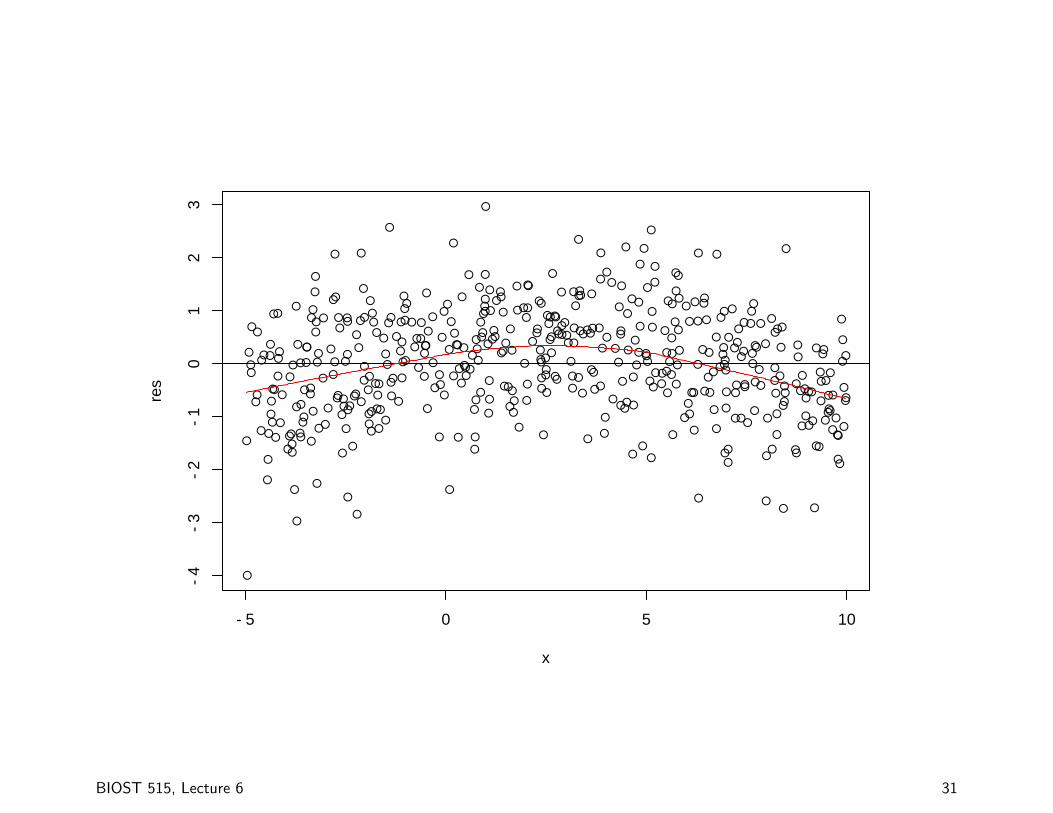
−5 0 5 10

−4

−3

−2

−1

01

23

x

res


●

●

●

●

●

●

●

●

●

●

●

●●

●

●

●

●

●

●

●

●

●

●

●● ●

●● ●

●

●

●

●

●

●

●

●

●●

●

●

●

●

●

●

●

●

● ●●

●

●

●

●

●

●

●

●

●

●

●

●

●

●

●

●

●

●

●

●

●

●

●

●

●

●

●

●

●

●

●

●

● ●

●●

●

●

●

●

●

●

●

●

●

●

●

●

●

●

●

●

●

●

●

●

●

●

●

●

●

●

●

●

●

●

●●

●

●

●

●●

●

●

●

●

●

●●

●

●

●

●●

●

●

●

●

●●

●

●

●

●

●●

●

●

●●

●

●

●

●●

●

●

●

●

●

●

●

●

●

●

●

●

●

●

●

●

●

●

●

●

●

●

●

●

●●

●

●●

●

●

●

●●

●●

●

●

●●

●

●●

●●

●

●

●

●

●●

●

●

●

● ●

●

●●

●

●

●●

●

●

●

●

●

●

●

●

●

●

●

●

●

●

●

●

●

●

●

●

●●

●

●

●

●

●

●

●

●●

●

●●

●

●

●

●●●

●

●

●

●

●

●

●

●

●●

●

●

●●

●

●

●

●

●

●

●

●

●

●

●

●●

●

●

●

●

●

●●

●

●

●

●

●

●

●

●

●

●

●●

●

●

●

●

● ●

●

●

●

●

●

●

●

●

●

●

●

●

●

●

●

●

●

●●

●

●●

●

●●

●

●

●

●

●

●●

●

●

●

●

●

●

●

●

●

●

●

●

●

●

●

●

●

●

●

●

●

●

●

●●

● ●

●

●

●

●

●

●

●●

●

●

●

●● ●

●

●

●

●

●

●

●

●

●●

●

●

●

●

●

●●●●

●

●

●

●

●

●

●

●

●

●

●●

●

●

●

●

●●

●

●

●

● ●

●

●

●

●

●

●

●

●

●

●

●●

●

●

●

●

●

●

●

●

●

●

●

●

●

●

●

●

●

●

●

●● ●

●

●

●

●

●

●

●

●

●●

● ●

●

●●

●

●

●

●

●

●

●

●

●

●

●

●

●

●●

●

●

●

●

●

●

●

●

●

●

2.0 2.5 3.0 3.5 4.0

−4

−3

−2

−1

01

23

w

res


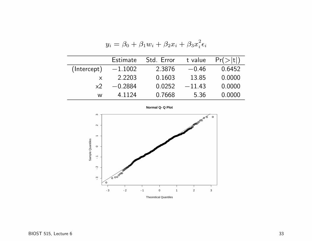
yi = β0 + β1wi + β2xi + β3x2i εi


x 2.2203 0.1603 13.85 0.0000

x2 −0.2884 0.0252 −11.43 0.0000

w 4.1124 0.7668 5.36 0.0000

●

●

●

●

●

●

●

●

●

●

●

●

●

●

●

●

●

●

●

●

●

●

●

●

●●

●●●

●

●

●

●

●

●

●

●

●

●

●

●

●

●

●

●

●

●

●●●

●

●

●

●

●

●

●

●

●

●

●

●

●

●

●

●

●

●

●

●

●

●

●

●●

●

●

●

●

●

●

●

●●

● ●

●

●

●

●

●

●

●

●

●

●

●

●●

●

●

●

●

●

●

●

●

●●

●

●

●

●●

●●

●●

●

●

●

●

●

●

●

●

●

●

●●

●

●

●

●●

●

●

●

●

●●●

●

●

●

●

●

●

●

●

●

●

●

●

●●

●

●

●

●●

●

●

●

●

●

●

●

●

●

●

●●

●

●

●

●

●

●

●

●

●

●

●

●

●

●

●

●●

●●

●●

●●●

●●

●

●

●

●

●

●

●

●

●

●

●

●

●

●

●

●

●●

●

●

●

●

●

●

●

●

●

●

●

●●●

●

●●

●

●

●

●

●

●

●

●●

●

●

●

●

●

●

●

●●

●

●

●

●

●

●

●

●

●

●

●

●

●

●

●

●

●

●

●

●●

●

●

●

●

●

●

●

●

●

●

●

●

●●

●

●

●

●

●

●

●

●

●

●

●

●

●

●●

●●

●

●●

●

●

●●

●

●

●

●

●

●

●

●

●

●

●

●

●

●

●

●

●

●

●

●

●

●●

●●

●

●

●

●

●●

●

●

●

●●

●

●

●

●

●

●

●

●

●

●

●

●

●

●

●

●

●

●

●

●●

●

●

●

●

●

●

●

●

●●

●

●

●

●

●●

●

●

●

●

●

●

●

●

●

●

●

●

●●

●

●

●

●

●

●

●

●●

●

●

●

●

●

●

●

●

●

●

●

●

●

●

●

●

●

●●

●

●

●

●

●

●

●

●

●

●

●●

●

●

●●

●

●

●

●

●

●

●

●●

●

●●

●

●

●

●

●

●

●●

●

●

●

●

●●

●

●

●●

●

●

●

●

●

●

●

●

●

●

●

●

●

●

●

●

●

●

●●

●

●

●

●

●

●

●

●

−3 −2 −1 0 1 2 3

−3

−2

−1

01

23

Normal Q−Q Plot


Sam

ple

Qua

ntile

s


●

●

●

●

●

●

●

●

●

●

●

●

●

●

●

●

●

●

●

●

●

●

●

●

● ●

● ●●

●

●

●

●

●

●

●

●

●

●

●

●

●

●

●

●

●

●

● ●●

●

●

●

●

●

●

●

●

●

●

●

●

●

●

●

●

●

●

●

●

●

●

●

●●

●

●

●

●

●

●

●

● ●

●●

●

●

●

●

●

●

●

●

●

●

●

●●

●

●

●

●

●

●

●

●

● ●

●

●

●

●●

● ●

●●

●

●

●

●

●

●

●

●

●

●

●●

●

●

●

●●

●

●

●

●

●● ●

●

●

●

●

●

●

●

●

●

●

●

●

●●

●

●

●

●●

●

●

●

●

●

●

●

●

●

●

● ●

●

●

●

●

●

●

●

●

●

●

●

●

●

●

●

●●

● ●

●●

●● ●

● ●

●

●

●

●

●

●

●

●

●

●

●

●

●

●

●

●

●●

●

●

●

●

●

●

●

●

●

●

●

●● ●

●

●●

●

●

●

●

●

●

●

●●

●

●

●

●

●

●

●

●●

●

●

●

●

●

●

●

●

●

●

●

●

●

●

●

●

●

●

●

●●

●

●

●

●

●

●

●

●

●

●

●

●

●●

●

●

●

●

●

●

●

●

●

●

●

●

●

●●

●●

●

● ●

●

●

●●

●

●

●

●

●

●

●

●

●

●

●

●

●

●

●

●

●

●

●

●

●

●●

●●

●

●

●

●

●●

●

●

●

●●

●

●

●

●

●

●

●

●

●

●

●

●

●

●

●

●

●

●

●

● ●

●

●

●

●

●

●

●

●

●●

●

●

●

●

● ●

●

●

●

●

●

●

●

●

●

●

●

●

● ●

●

●

●

●

●

●

●

●●

●

●

●

●

●

●

●

●

●

●

●

●

●

●

●

●

●

●●

●

●

●

●

●

●

●

●

●

●

●●

●

●

●●

●

●

●

●

●

●

●

●●

●

●●

●

●

●

●

●

●

● ●

●

●

●

●

●●

●

●

●●

●

●

●

●

●

●

●

●

●

●

●

●

●

●

●

●

●

●

●●

●

●

●

●

●

●

●

●

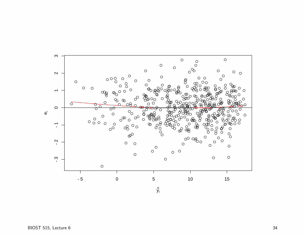
−5 0 5 10 15

−3

−2

−1

01

23

yi

e i


Partial regression plots

• A variation of the plot of residuals versus predictors

• Allows us to study the marginal relationship of a regressor

given the other variables that are in the model.

• Also called the added variable plot or the adjusted variableplot


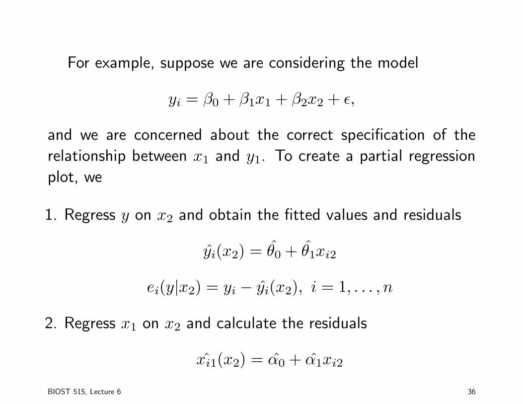
For example, suppose we are considering the model

yi = β0 + β1x1 + β2x2 + ε,

and we are concerned about the correct specification of the

relationship between x1 and y1. To create a partial regression

plot, we

1. Regress y on x2 and obtain the fitted values and residuals

yi(x2) = θ0 + θ1xi2

ei(y|x2) = yi − yi(x2), i = 1, . . . , n

2. Regress x1 on x2 and calculate the residuals

xi1(x2) = α0 + α1xi2


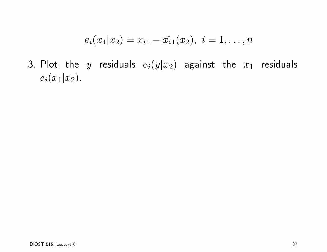
ei(x1|x2) = xi1 − xi1(x2), i = 1, . . . , n

3. Plot the y residuals ei(y|x2) against the x1 residuals

ei(x1|x2).


Partial regression plot from previous example

●

●

●

●

●

●

●

●

●

●●

●

●

●

●

●

●

●

●

●

●

●●

●

●

●

●

●

●

●

●

●

●●

●●

●

●

●

●

●

●

●●

●

●

●●

●

●

●

●

●

●

●

●

●

●

●

●

●

●

●●

●

●

●

● ●

●

●

●

●

●

●

●

●

●

●

●

●

●

●

●

●●

●

●

●

●

●

●

●●

●

● ●●

●

●

●

●

●

●

●●●

●●

●

●

●

●

●

●

●

●●

●

●●

●●

●

●

●

●

●

●

●

●

●●

●

●

●

●●

●

●

●

●

●●●

●

●

●

●

●

●

●

●

●

●

●

●

● ● ●

●

●●

●●

●

●

●

●

●

●

●●

●

●●

●

●●

●

●

●

●

●

●

●

●

●●

●

●

●

●

●

●●

● ●

●

●

●

●

●

●

●

●

●

●

●

●●

●

●

●

●

●

●

●

●

●

●●

●

●

●

●

●

●

● ●

●●

●●

●

●

●

●

●

●

●

●●

●

●

●

●

●

●

●

●

●

●

●

●

●

●

●

●

●

●

●

●

●

●

●

●

●

●●

●

●

●

●

●

●

●

●●

●

●

●

●

●

●

●

● ●

●

●

●

●

●

●

●

●

●

●

●●

●

●

●

●

●

●

●●

●

●

●

●

●

●

●

●

●

●

●

●

●

●

●

●

●

●● ●

●

●

●

●

●

●

●

●

●

●●

●

●

●

●

● ●

●

●

●

●

●

●

●

●

●

●

●

●

●

●

●

●

●

●

●●

●

●

●

●

●

●

●

●●●

●

●

●●

●

●

●

●

●

●

●

●

●

●

●●

●

●

●

●

●

●

●

●

●

●

●

●

●

●

●

●●

●

●

●

●

●

●

●

●

●

●

●

●

●

●●

●

●

●

●

●

●

●●

●

●

●

●

●

●

●

●

●

●

●

●

●

●●

●

●

●

●

●

●

●

●

●

●

●

●

●

●

●●

●

●

●

●

●●

●

●

●

●

●

●

●

●

●●

●

● ●●

●

●

●

●

●● ●

●

●

● ●●

●

●

●

●

●

●

−5 0 5

−40

−30

−20

−10

010

20

x

y


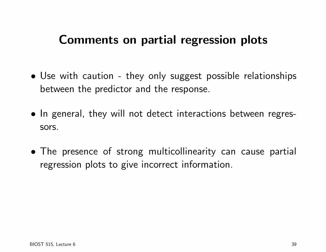
Comments on partial regression plots

• Use with caution - they only suggest possible relationships

between the predictor and the response.

• In general, they will not detect interactions between regres-

sors.

• The presence of strong multicollinearity can cause partial

regression plots to give incorrect information.


Next

• Variance stabilizing transformations

• Identifying outliers and influential observations.


lecture 7 linear regression diagnosticscourses.washington.edu/b515/l7.pdf · lecture 7 linear...

Documents