Lecture 7: Irrigation Systems

Prepared by

Husam Al-Najar

The Islamic University of Gaza- Civil Engineering Department

Irrigation and Drainage- ECIV 5327

Surface Irrigation

Surface Irrigation

• Water flows across the soil surface to the point of infiltration

• Oldest irrigation method and most widely used world-wide (90%)

• Used primarily on agricultural or orchard crops

Types of Systems

• Water Spreading or Wild Flooding

– Relatively flat fields -- allow water to find its own way across the surface

– Minimal preparation and investment

• Basin

– Dikes used to surround an area and allow for water ponding (no runoff)

– Basins are usually level

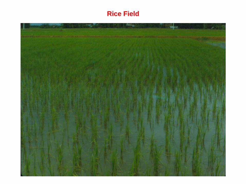
Rice Field

Types of Systems, Contd…

• Border

– Strips of land with dikes on the sides

– Usually graded but with no cross slope

– Downstream end may be diked

• Furrow

– Small channels carry the water

– Commonly used on row crops

– Lateral as well as vertical infiltration

– Furrows are usually graded

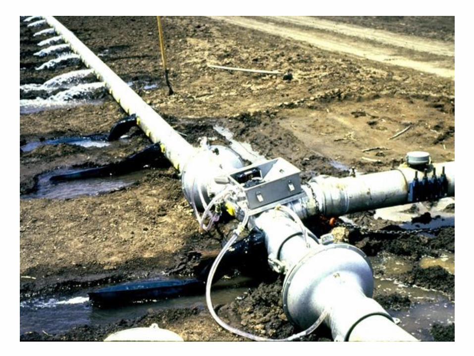
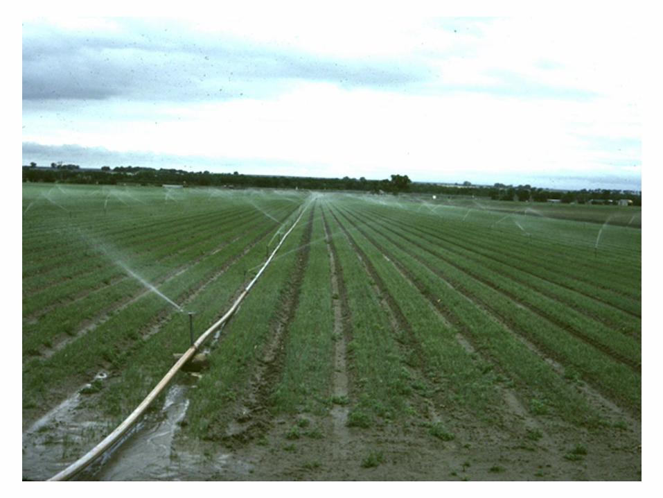
Water Supply

• Methods of water supply

– Head ditch with siphon tubes or side-opening gates

– Gated pipe (aluminum or plastic pipe with small gates that can be opened

and closed)

– Buried pipeline with periodically spaced valves at the surface

Water Management

• Runoff recovery systems

– Drainage ditches for collecting and conveying runoff to the reservoir

– Reservoir for storing the runoff water

– Inlet facilities to the reservoir

– Pump and power unit

– Conveyance system for transporting water (to same or different field)

Runoff recovery systems

Surface Irrigation Hydraulics

• Advance :Movement of water from the inlet end to the downstream end.

– Curve of Time vs. Distance is NOT linear

– Rule-of-Thumb: 1/3 of the total advance time is needed to reach midpoint

of the furrow length

• Recession (التوقف/الركود): Process of water leaving the surface (through

infiltration and/or runoff) after the inflow has been cut off

– Usually begins to recede at the upstream end

– Can also be plotted as Time vs. Distance

– “Flatter" curve than the Advance Curve

Surface Irrigation Hydraulics, Cont’d

• Infiltration

– Opportunity Time: difference between Recession and Advance

curves

– Infiltration Depth: a function of the opportunity time and the infiltration

rate of the soil

Curve of Time Vs. Distance

Distance from inlet end (ft)

Opportunity Time

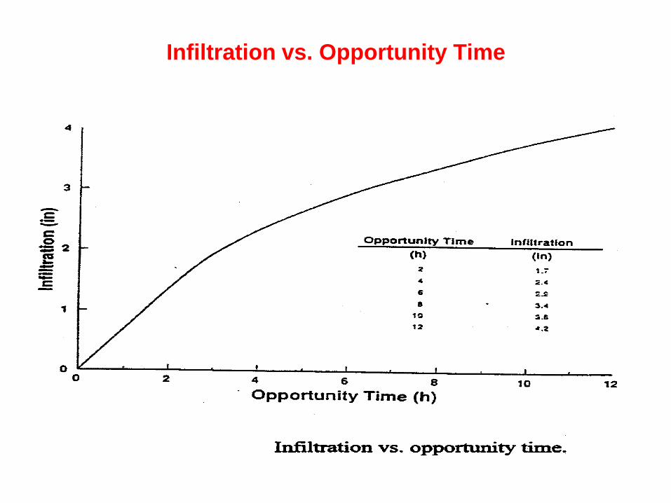
Infiltration vs. Opportunity Time

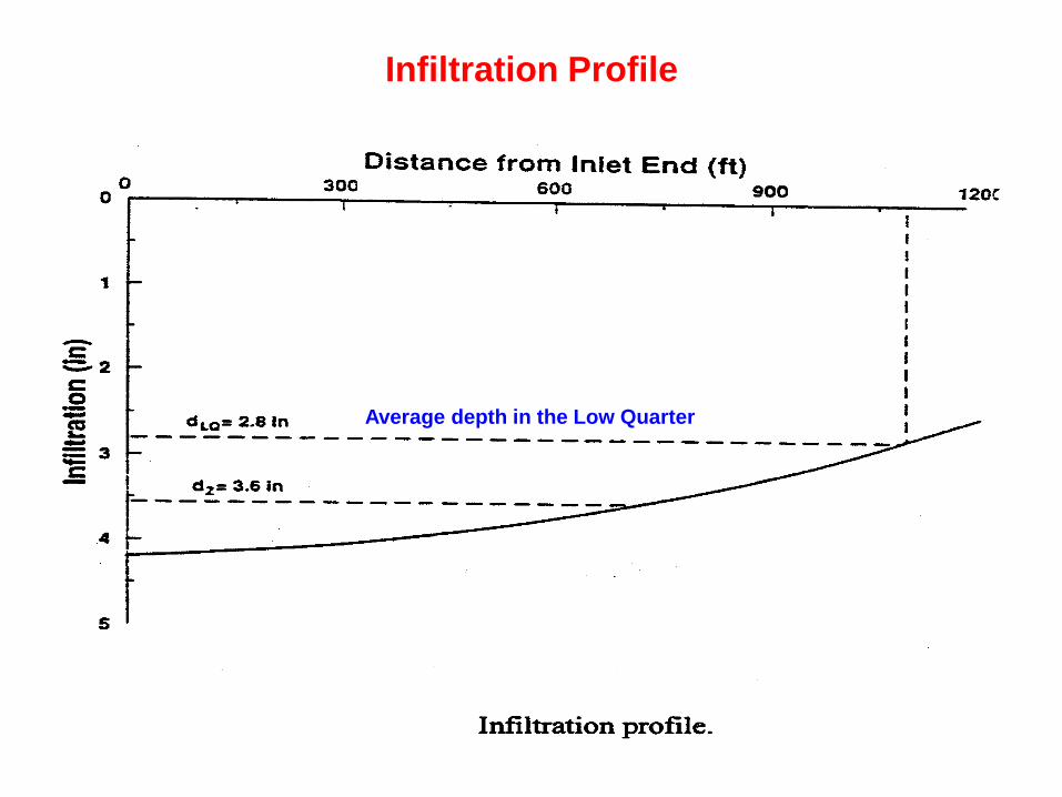
Infiltration Profile

Average depth in the Low Quarter

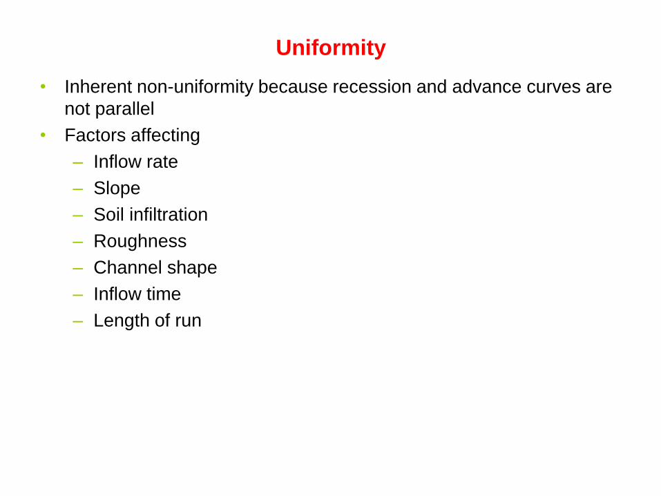
Uniformity

• Inherent non-uniformity because recession and advance curves are

not parallel

• Factors affecting

– Inflow rate

– Slope

– Soil infiltration

– Roughness

– Channel shape

– Inflow time

– Length of run

Efficiency

• Volume balance

– Vg = Vz + Vs + Vr

– g gross

– z infiltration

– s surface storage

– r runoff

• (or depth basis): dg = dz + ds + dr

• Part of infiltration may go to deep percolation

Calculating dg (Gross Application Depth)

• Single furrow:

• Furrow set:

• Basin/border:

dq t

WLg

s co

1155

NWL

Qtd co

g 1155

dQt

W Lg

co

b b

96 3.

W= spacing between raw, L= Length of raw, N= number of raw, Wb= basin width

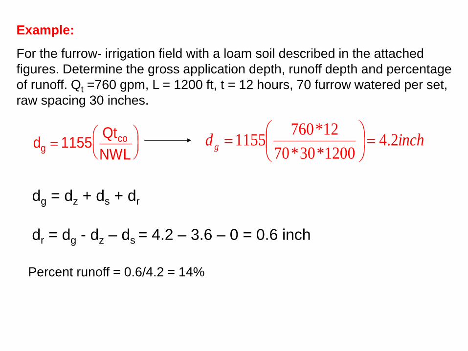
Example:

For the furrow- irrigation field with a loam soil described in the attached

figures. Determine the gross application depth, runoff depth and percentage

of runoff. Qt =760 gpm, L = 1200 ft, t = 12 hours, 70 furrow watered per set,

raw spacing 30 inches.

dQt

NWLg

co

1155 inchd g 2.4

1200*30*70

12*7601155

dg = dz + ds + dr

dr = dg - dz – ds = 4.2 – 3.6 – 0 = 0.6 inch

Percent runoff = 0.6/4.2 = 14%

Average depth in the Low Quarter

Micro-irrigation

Microirrigation

• Delivery of water at low flow rates through various types of water applicators by

a distribution system located on the soil surface, beneath the surface, or

suspended above the ground

• Water is applied as drops, tiny streams, or spray, through emitters, sprayers, or

porous tubing

Water Application Characteristics

• Low rates

• Over long periods of time

• At frequent intervals

• Near or directly into the root zone

• At low pressure

• Usually maintain relatively high water content

• Used on higher value agricultural/horticultural crops and in

landscapes and nurseries

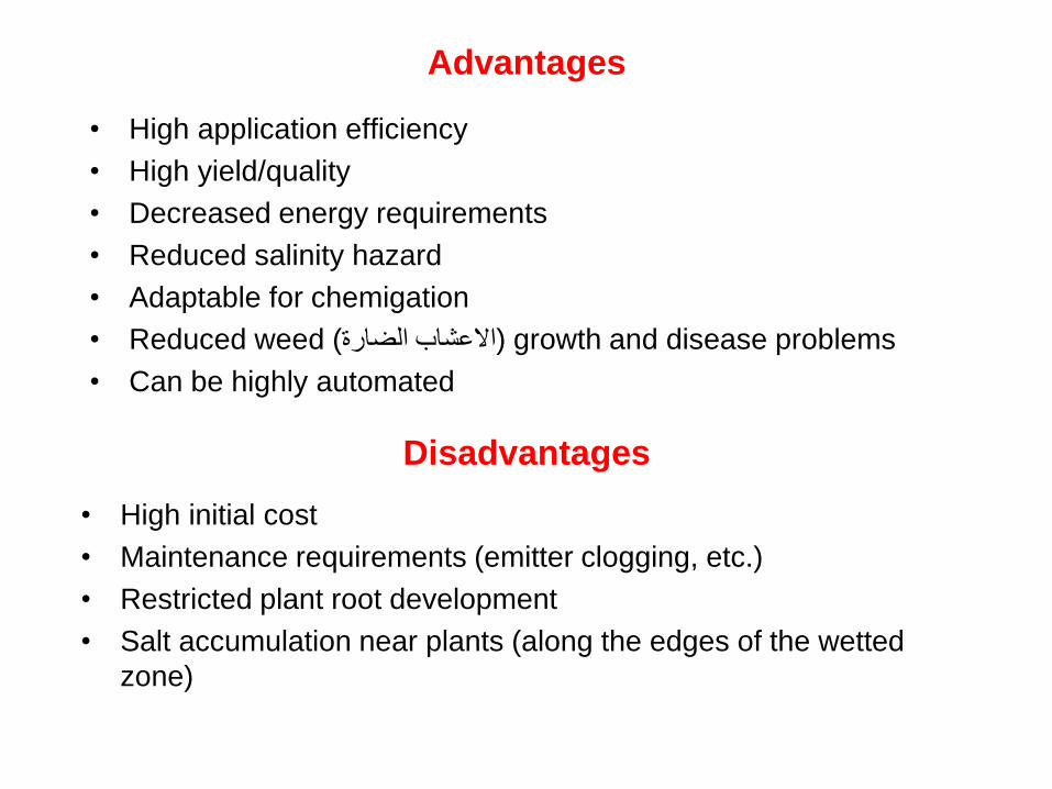
Advantages

• High application efficiency

• High yield/quality

• Decreased energy requirements

• Reduced salinity hazard

• Adaptable for chemigation

• Reduced weed (االعشاب الضارة) growth and disease problems

• Can be highly automated

Disadvantages

• High initial cost

• Maintenance requirements (emitter clogging, etc.)

• Restricted plant root development

• Salt accumulation near plants (along the edges of the wetted

zone)

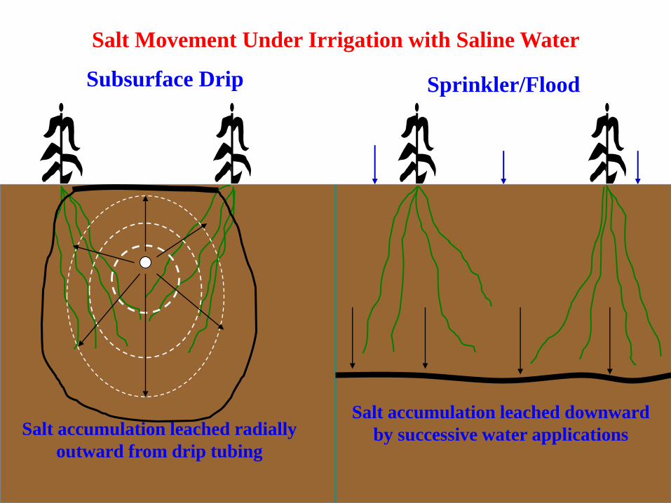
Salt Movement Under Irrigation with Saline Water

Salt accumulation leached downward

by successive water applications Salt accumulation leached radially

outward from drip tubing

Subsurface Drip Sprinkler/Flood

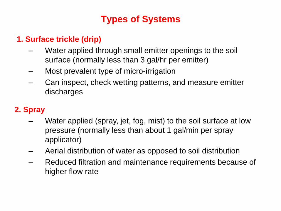
Types of Systems

1. Surface trickle (drip)

– Water applied through small emitter openings to the soil

surface (normally less than 3 gal/hr per emitter)

– Most prevalent type of micro-irrigation

– Can inspect, check wetting patterns, and measure emitter

discharges

2. Spray

– Water applied (spray, jet, fog, mist) to the soil surface at low

pressure (normally less than about 1 gal/min per spray

applicator)

– Aerial distribution of water as opposed to soil distribution

– Reduced filtration and maintenance requirements because of

higher flow rate

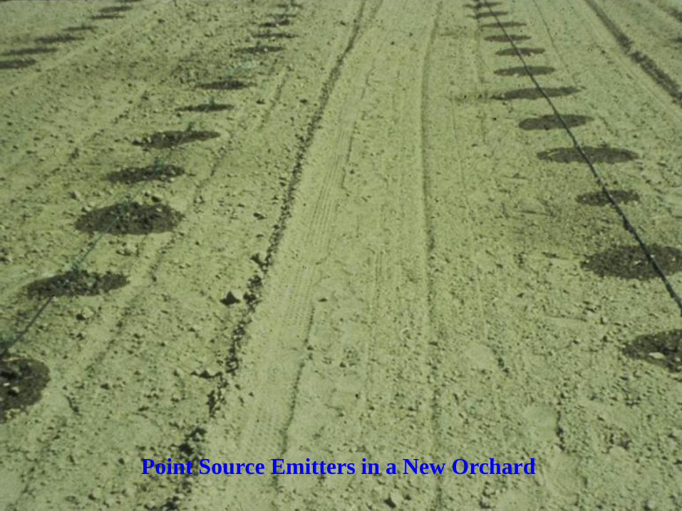
Point Source Emitters in a New Orchard

3. Bubbler

– Water applied as a small stream to flood the soil surface in

localized areas (normally less than about 1 gal/min per discharge

point)

– Application rate usually greater than the soil's infiltration rate

(because of small wetted diameter)

– Minimal filtration and maintenance requirements

4. Subsurface trickle

– Water applied through small emitter openings below the soil surface

– Basically a surface system that's been buried (few inches to a

couple feet)

– Permanent installation that is "out of the way"

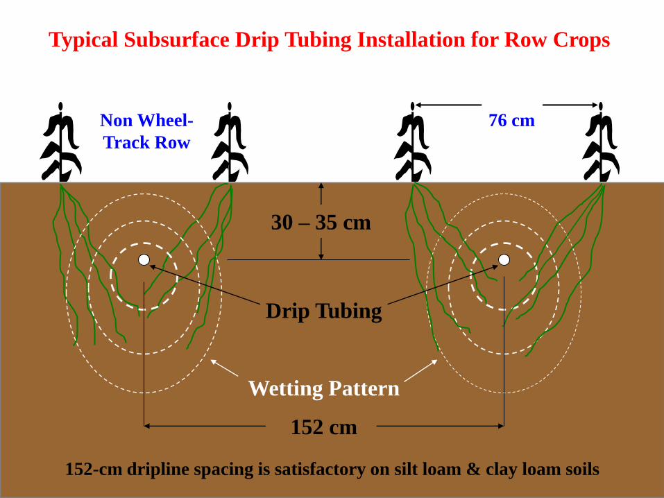
76 cm

152 cm

Typical Subsurface Drip Tubing Installation for Row Crops

30 – 35 cm

Non Wheel-

Track Row

Wetting Pattern

Drip Tubing

152-cm dripline spacing is satisfactory on silt loam & clay loam soils

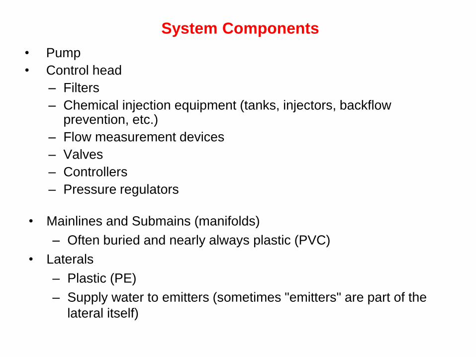
System Components

• Pump

• Control head

– Filters

– Chemical injection equipment (tanks, injectors, backflow prevention, etc.)

– Flow measurement devices

– Valves

– Controllers

– Pressure regulators

• Mainlines and Submains (manifolds)

– Often buried and nearly always plastic (PVC)

• Laterals

– Plastic (PE)

– Supply water to emitters (sometimes "emitters" are part of the

lateral itself)

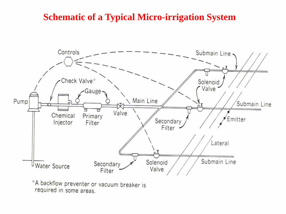
Schematic of a Typical Micro-irrigation System

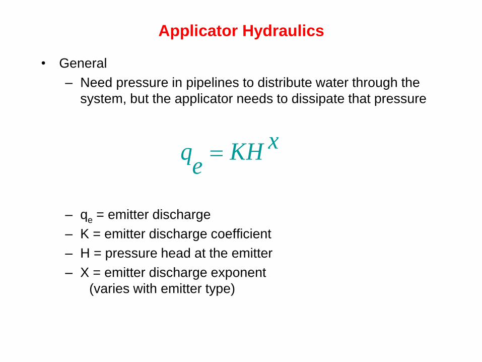
Applicator Hydraulics

• General

– Need pressure in pipelines to distribute water through the

system, but the applicator needs to dissipate that pressure

– qe = emitter discharge

– K = emitter discharge coefficient

– H = pressure head at the emitter

– X = emitter discharge exponent

(varies with emitter type)

xKHe

q

Emitter Hydraulics

Emitter Type

Coefficient, K - Exponent, X

Emitter Discharge (Liter/minute)

Operating Pressure (m)

5.6 m

8.4 m

11.2 m

Porous Pipe - 0.112 1.00

9.0

13.6

18.2

Tortuous Path 0.112 0.65

3.3

4.3

5.2

Vortex/Orifice 0.112 0.42

1.7

2.0

2.2

Compensating 0.112 0.20

0.9

0.9

1.0

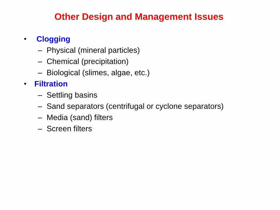
Other Design and Management Issues

• Clogging

– Physical (mineral particles)

– Chemical (precipitation)

– Biological (slimes, algae, etc.)

• Filtration

– Settling basins

– Sand separators (centrifugal or cyclone separators)

– Media (sand) filters

– Screen filters

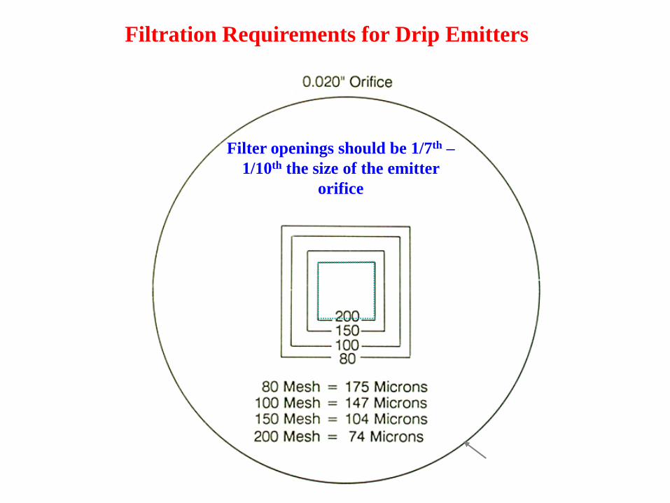
Filtration Requirements for Drip Emitters

Filter openings should be 1/7th –

1/10th the size of the emitter

orifice

0.020-inch orifice

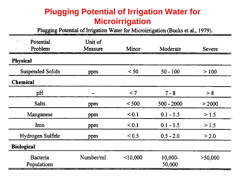
Plugging Potential of Irrigation Water for

Microirrigation

• Chemical treatment

– Acid: prevent calcium precipitation

– Chlorine

• control biological activity: algae and bacterial slime

• deliberately precipitate iron

• Flushing

– after installation or repairs, and as part of routine maintenance

– valves or other openings at the end of all pipes, including laterals

• Application uniformity

– manufacturing variation

– pressure variations in the mainlines and laterals

– pressure-discharge relationships of the applicators

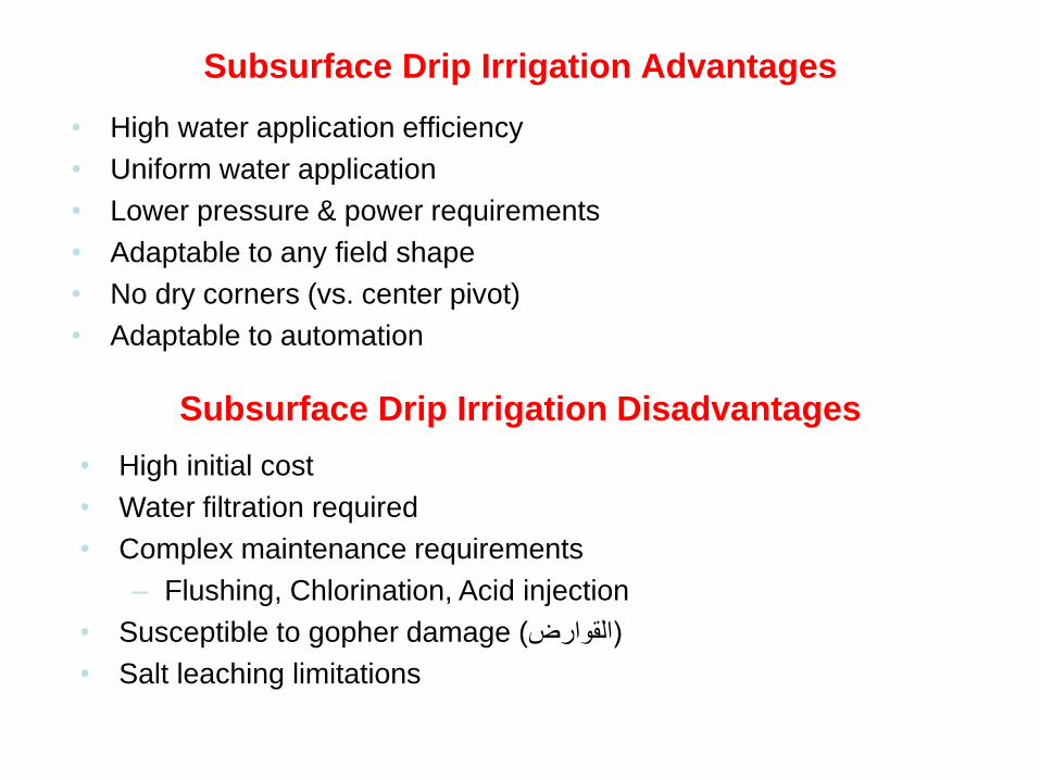
Subsurface Drip Irrigation Advantages

• High water application efficiency

• Uniform water application

• Lower pressure & power requirements

• Adaptable to any field shape

• No dry corners (vs. center pivot)

• Adaptable to automation

Subsurface Drip Irrigation Disadvantages

• High initial cost

• Water filtration required

• Complex maintenance requirements

– Flushing, Chlorination, Acid injection

• Susceptible to gopher damage ( القوارض(

• Salt leaching limitations

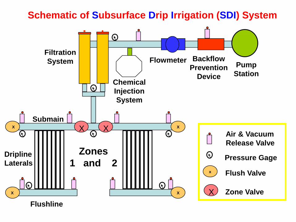
Schematic of Subsurface Drip Irrigation (SDI) System

Pump

Station

Backflow

Prevention

Device

Flowmeter

Chemical

Injection

System

Air & Vacuum

Release Valve

X X

Pressure Gage

X X

Flush Valve

X X

Dripline

Laterals

Zones

1 and 2

Submain

Flushline

Filtration

System

x

X Zone Valve

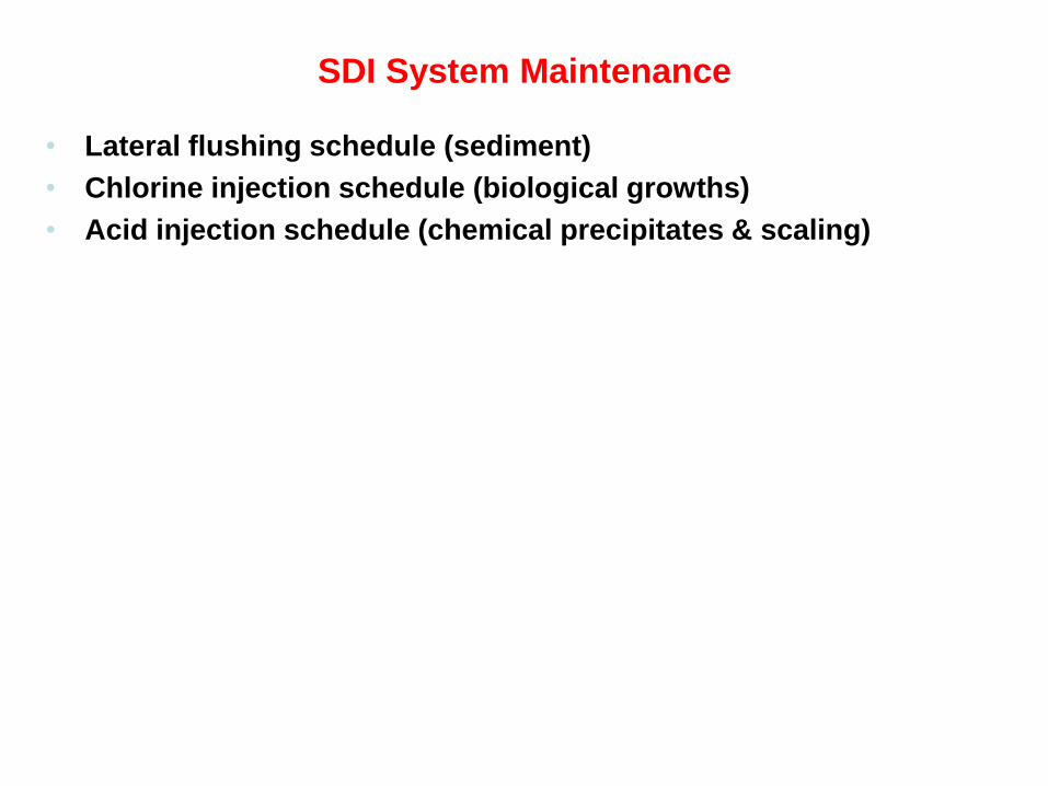
SDI System Maintenance

• Lateral flushing schedule (sediment)

• Chlorine injection schedule (biological growths)

• Acid injection schedule (chemical precipitates & scaling)

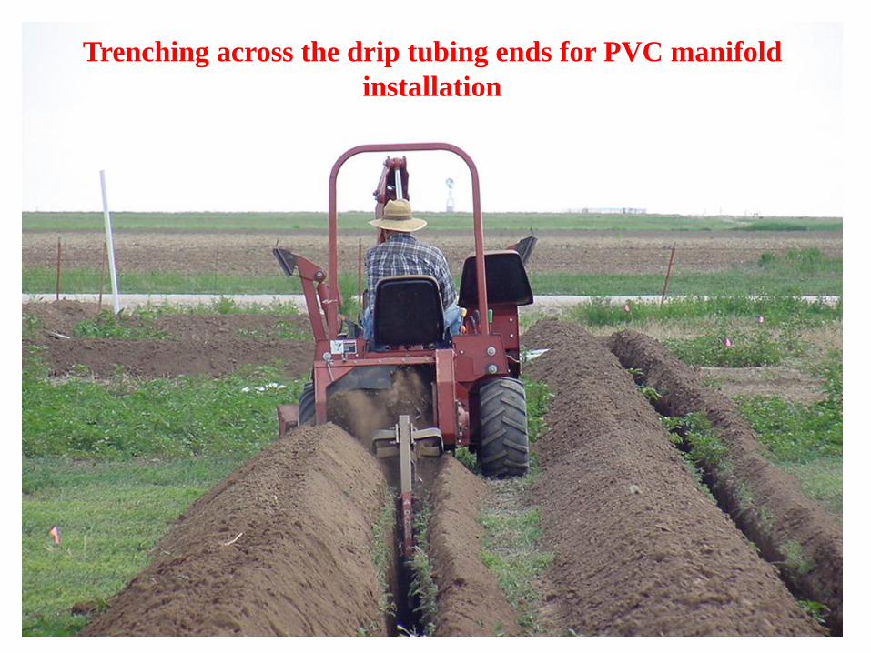
Trenching across the drip tubing ends for PVC manifold

installation

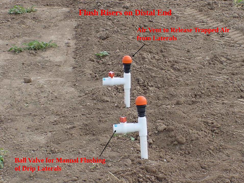
Flush Risers on Distal End

Ball Valve for Manual Flushing

of Drip Laterals

Air Vent to Release Trapped Air

from Laterals

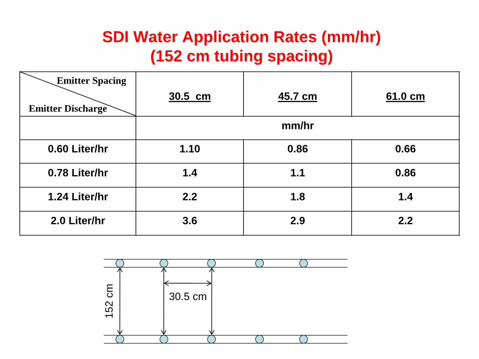
SDI Water Application Rates (mm/hr)

(152 cm tubing spacing)

cm30.5

cm45.7

cm61.0

mm/hr

0.60 Liter/hr 1.10 0.86 0.66

0.78 Liter/hr 1.4 1.1 0.86

1.24 Liter/hr 2.2 1.8 1.4

2.0 Liter/hr 3.6 2.9 2.2

Emitter Spacing

Emitter Discharge 1

52

cm

30.5 cm

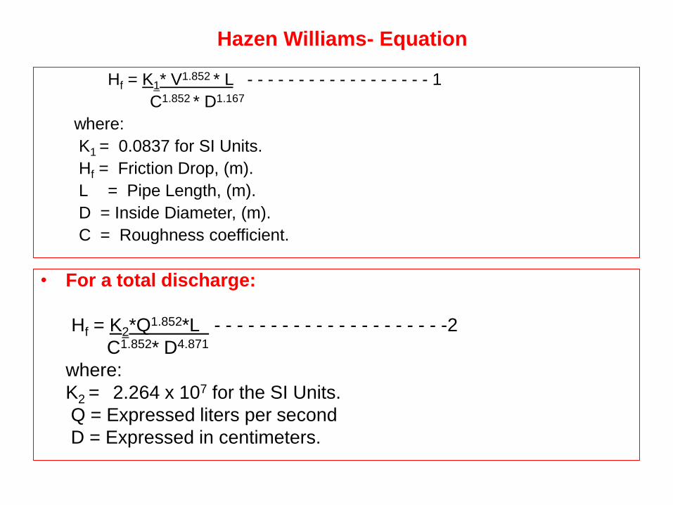
Hazen Williams- Equation

Hf = K1* V1.852 * L - - - - - - - - - - - - - - - - - - 1

C1.852 * D1.167

where:

K1 = 0.0837 for SI Units.

Hf = Friction Drop, (m).

L = Pipe Length, (m).

D = Inside Diameter, (m).

C = Roughness coefficient.

• For a total discharge:

Hf = K2*Q1.852*L - - - - - - - - - - - - - - - - - - - - -2

C1.852* D4.871

where:

K2 = 2.264 x 107 for the SI Units.

Q = Expressed liters per second

D = Expressed in centimeters.

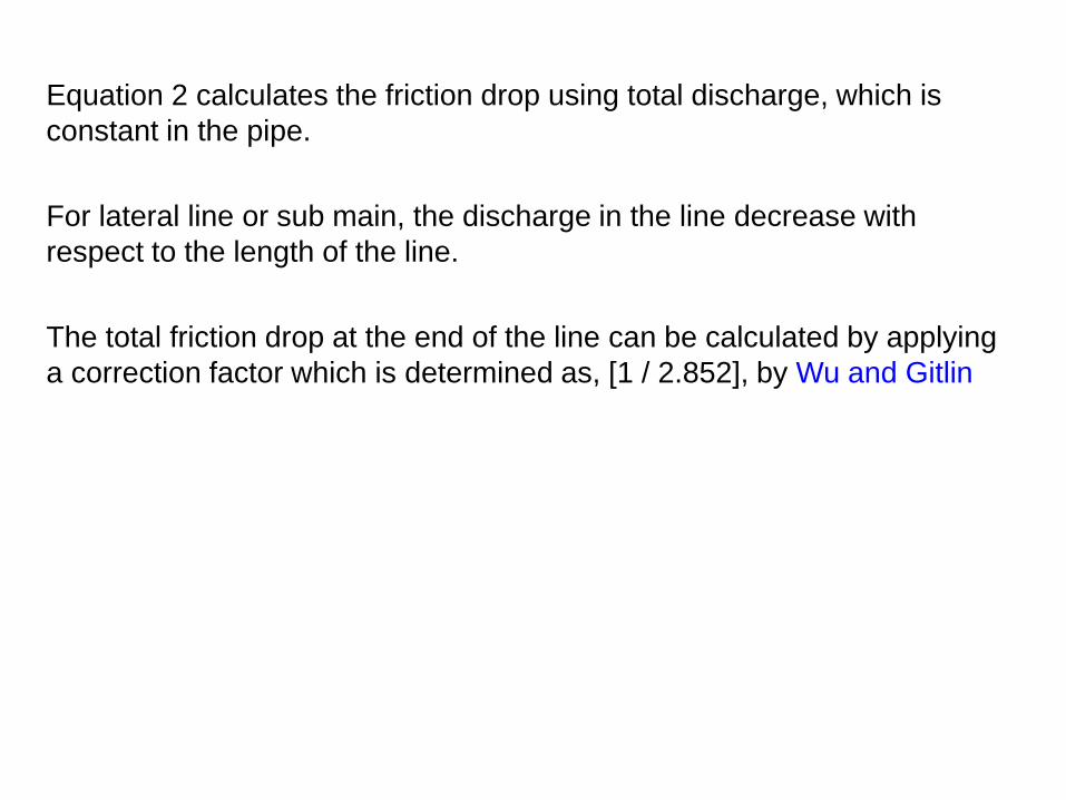
Equation 2 calculates the friction drop using total discharge, which is

constant in the pipe.

For lateral line or sub main, the discharge in the line decrease with

respect to the length of the line.

The total friction drop at the end of the line can be calculated by applying

a correction factor which is determined as, [1 / 2.852], by Wu and Gitlin

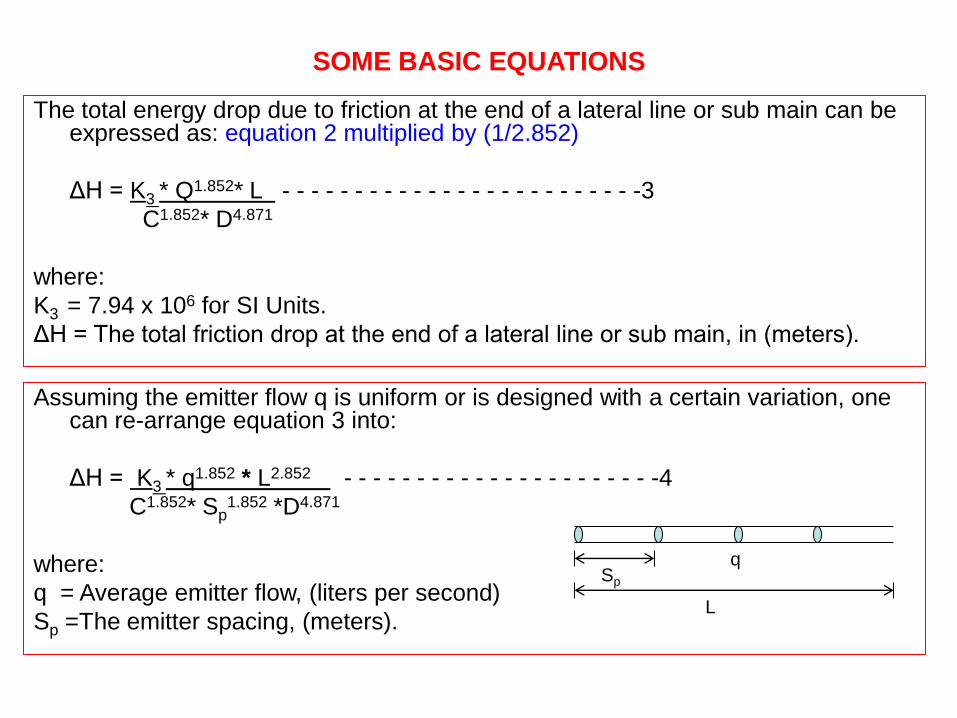
SOME BASIC EQUATIONS

The total energy drop due to friction at the end of a lateral line or sub main can be expressed as: equation 2 multiplied by (1/2.852)

ΔH = K3 * Q1.852* L - - - - - - - - - - - - - - - - - - - - - - - - -3

C1.852* D4.871

where:

K3 = 7.94 x 106 for SI Units.

ΔH = The total friction drop at the end of a lateral line or sub main, in (meters).

Assuming the emitter flow q is uniform or is designed with a certain variation, one can re-arrange equation 3 into:

ΔH = K3 * q1.852 * L2.852 - - - - - - - - - - - - - - - - - - - - - -4

C1.852* Sp1.852 *D4.871

where:

q = Average emitter flow, (liters per second)

Sp =The emitter spacing, (meters).

Sp

L

q

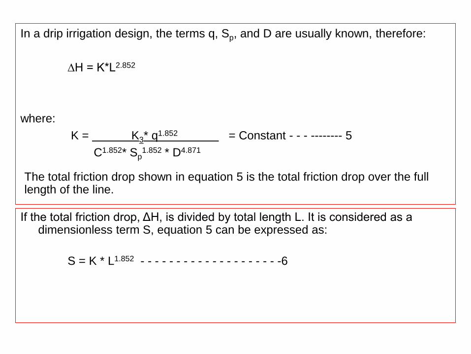
In a drip irrigation design, the terms q, Sp, and D are usually known, therefore:

∆H = K*L2.852

where:

K = K3* q1.852 = Constant - - - -------- 5

C1.852* Sp1.852 * D4.871

If the total friction drop, ΔH, is divided by total length L. It is considered as a dimensionless term S, equation 5 can be expressed as:

S = K * L1.852 - - - - - - - - - - - - - - - - - - - -6

The total friction drop shown in equation 5 is the total friction drop over the full length of the line.

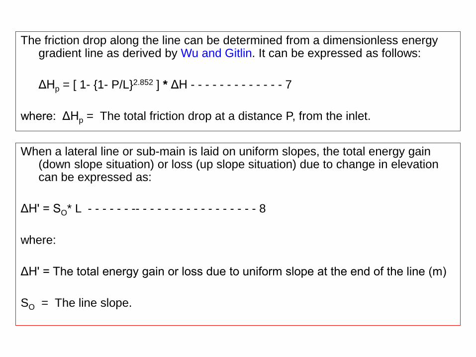
The friction drop along the line can be determined from a dimensionless energy gradient line as derived by Wu and Gitlin. It can be expressed as follows:

ΔHp = [ 1- {1- P/L}2.852 ] * ΔH - - - - - - - - - - - - - 7

where: ΔHp = The total friction drop at a distance P, from the inlet.

When a lateral line or sub-main is laid on uniform slopes, the total energy gain (down slope situation) or loss (up slope situation) due to change in elevation can be expressed as:

ΔH' = SO* L - - - - - - -- - - - - - - - - - - - - - - - - 8

where:

ΔH' = The total energy gain or loss due to uniform slope at the end of the line (m)

SO = The line slope.

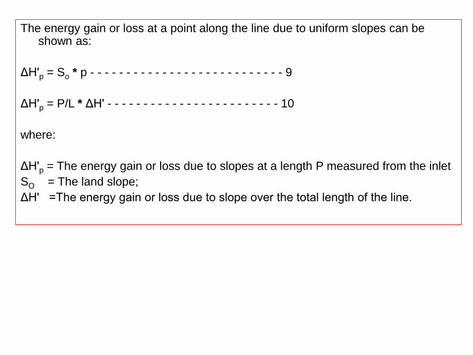
The energy gain or loss at a point along the line due to uniform slopes can be shown as:

ΔH'p = So * p - - - - - - - - - - - - - - - - - - - - - - - - - - - 9

ΔH'p = P/L * ΔH' - - - - - - - - - - - - - - - - - - - - - - - - 10

where:

ΔH'p = The energy gain or loss due to slopes at a length P measured from the inlet

SO = The land slope;

ΔH' =The energy gain or loss due to slope over the total length of the line.

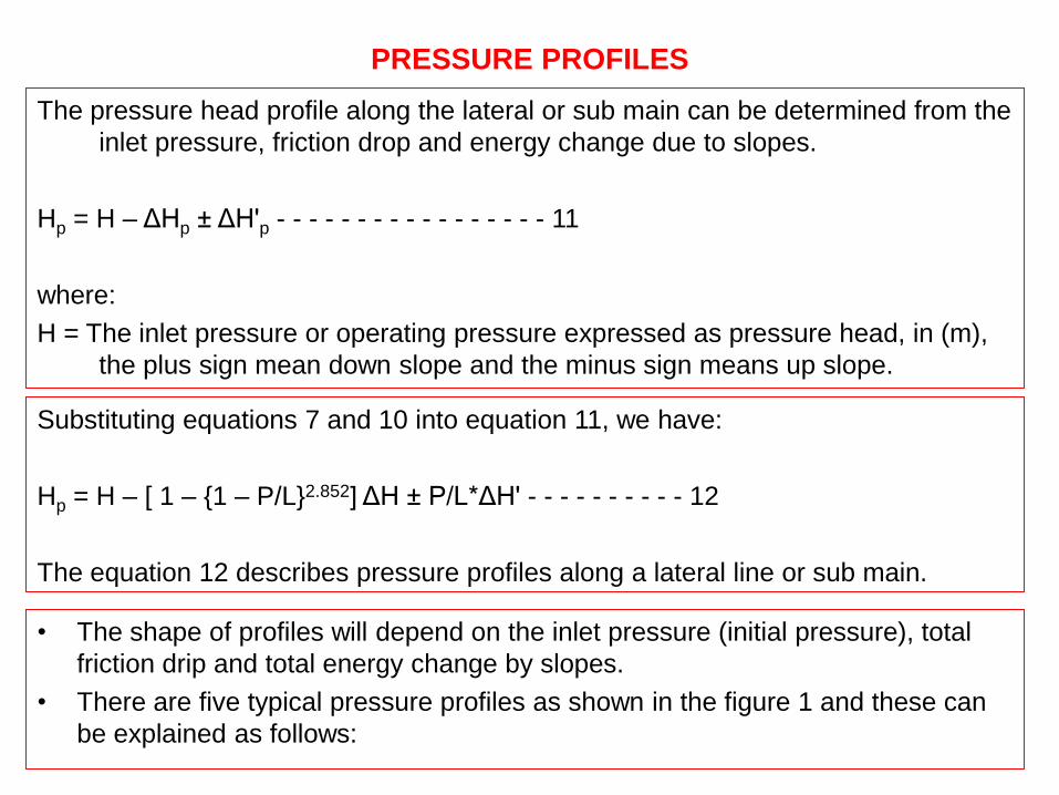
PRESSURE PROFILES

The pressure head profile along the lateral or sub main can be determined from the

inlet pressure, friction drop and energy change due to slopes.

Hp = H – ΔHp ± ΔH'p - - - - - - - - - - - - - - - - - 11

where:

H = The inlet pressure or operating pressure expressed as pressure head, in (m),

the plus sign mean down slope and the minus sign means up slope.

Substituting equations 7 and 10 into equation 11, we have:

Hp = H – [ 1 – {1 – P/L}2.852] ΔH ± P/L*ΔH' - - - - - - - - - - 12

The equation 12 describes pressure profiles along a lateral line or sub main.

• The shape of profiles will depend on the inlet pressure (initial pressure), total

friction drip and total energy change by slopes.

• There are five typical pressure profiles as shown in the figure 1 and these can

be explained as follows:

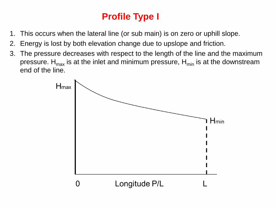
Profile Type I

1. This occurs when the lateral line (or sub main) is on zero or uphill slope.

2. Energy is lost by both elevation change due to upslope and friction.

3. The pressure decreases with respect to the length of the line and the maximum

pressure. Hmax is at the inlet and minimum pressure, Hmin is at the downstream

end of the line.

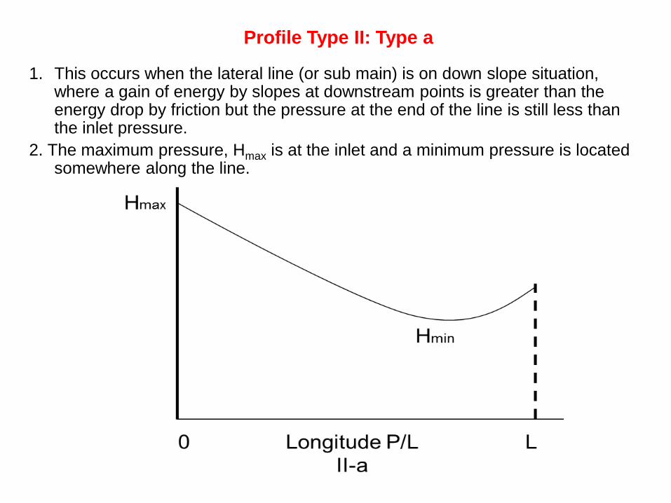
Profile Type II: Type a

1. This occurs when the lateral line (or sub main) is on down slope situation, where a gain of energy by slopes at downstream points is greater than the energy drop by friction but the pressure at the end of the line is still less than the inlet pressure.

2. The maximum pressure, Hmax is at the inlet and a minimum pressure is located somewhere along the line.

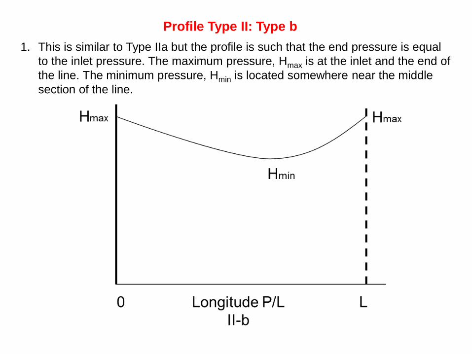
Profile Type II: Type b

1. This is similar to Type IIa but the profile is such that the end pressure is equal

to the inlet pressure. The maximum pressure, Hmax is at the inlet and the end of

the line. The minimum pressure, Hmin is located somewhere near the middle

section of the line.

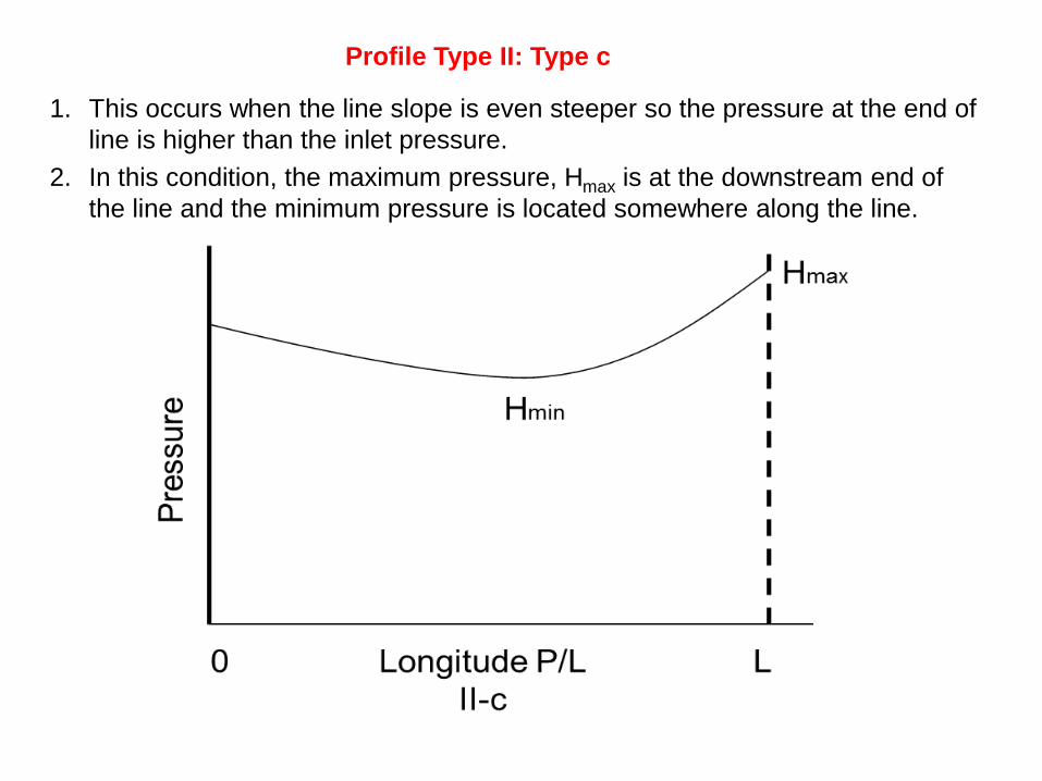
Profile Type II: Type c

1. This occurs when the line slope is even steeper so the pressure at the end of

line is higher than the inlet pressure.

2. In this condition, the maximum pressure, Hmax is at the downstream end of

the line and the minimum pressure is located somewhere along the line.

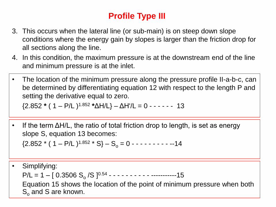
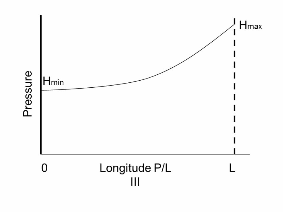
Profile Type III

3. This occurs when the lateral line (or sub-main) is on steep down slope

conditions where the energy gain by slopes is larger than the friction drop for

all sections along the line.

4. In this condition, the maximum pressure is at the downstream end of the line

and minimum pressure is at the inlet.

• The location of the minimum pressure along the pressure profile II-a-b-c, can

be determined by differentiating equation 12 with respect to the length P and

setting the derivative equal to zero.

{2.852 * ( 1 – P/L )1.852 *ΔH/L} – ΔH'/L = 0 - - - - - - 13

• If the term ΔH/L, the ratio of total friction drop to length, is set as energy

slope S, equation 13 becomes:

{2.852 * ( 1 – P/L )1.852 * S} – So = 0 - - - - - - - - - --14

• Simplifying:

P/L = 1 – [ 0.3506 So /S ]0.54 - - - - - - - - - - -----------15

Equation 15 shows the location of the point of minimum pressure when both So and S are known.

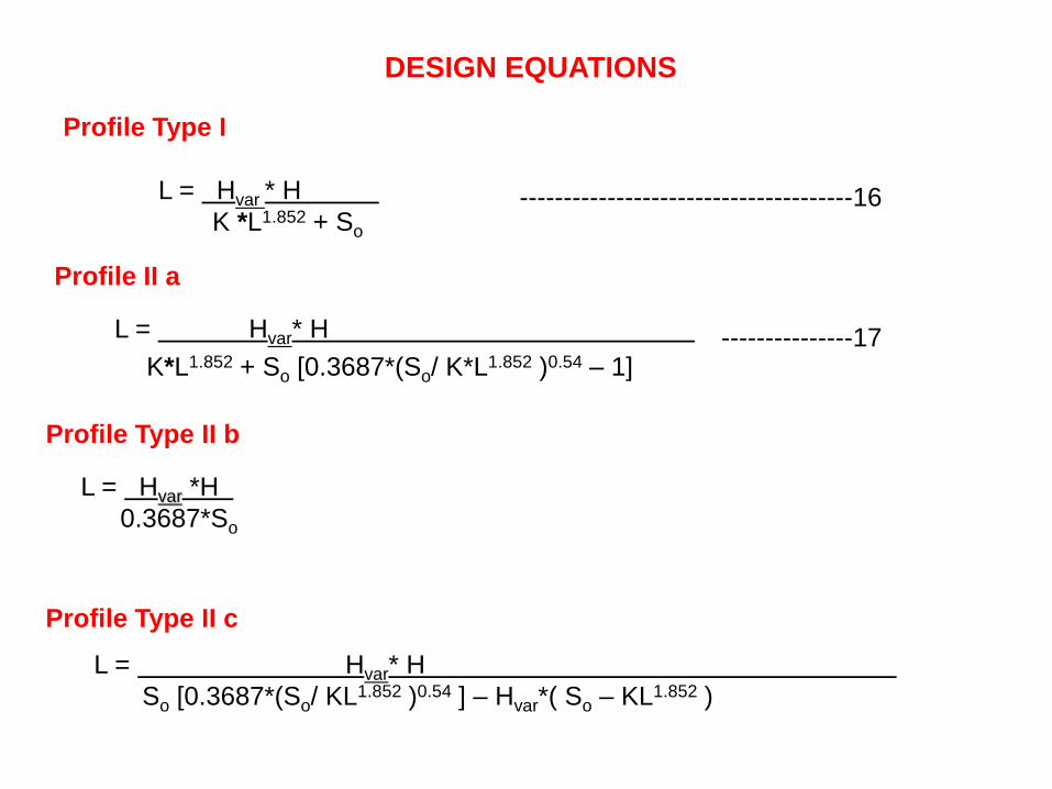
DESIGN EQUATIONS

Profile Type I

L = Hvar * H

K *L1.852 + So

Profile II a

L = Hvar* H

K*L1.852 + So [0.3687*(So/ K*L1.852 )0.54 – 1]

Profile Type II b

L = Hvar *H

0.3687*So

Profile Type II c

L = Hvar* H

So [0.3687*(So/ KL1.852 )0.54 ] – Hvar*( So – KL1.852 )

--------------------------------------16

---------------17

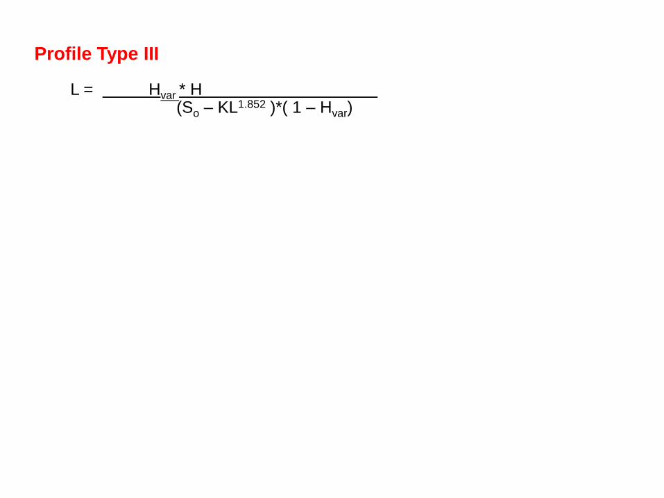
Profile Type III

L = Hvar * H (So – KL1.852 )*( 1 – Hvar)

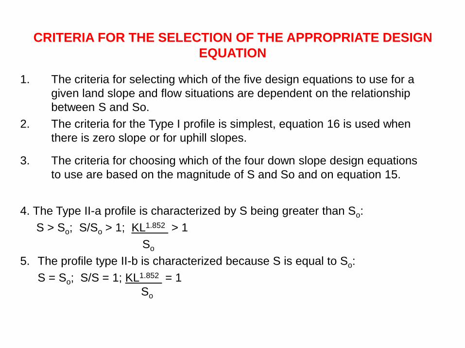
CRITERIA FOR THE SELECTION OF THE APPROPRIATE DESIGN

EQUATION

1. The criteria for selecting which of the five design equations to use for a

given land slope and flow situations are dependent on the relationship

between S and So.

2. The criteria for the Type I profile is simplest, equation 16 is used when

there is zero slope or for uphill slopes.

3. The criteria for choosing which of the four down slope design equations

to use are based on the magnitude of S and So and on equation 15.

4. The Type II-a profile is characterized by S being greater than So:

S > So; S/So > 1; KL1.852 > 1

So

5. The profile type II-b is characterized because S is equal to So:

S = So; S/S = 1; KL1.852 = 1

So

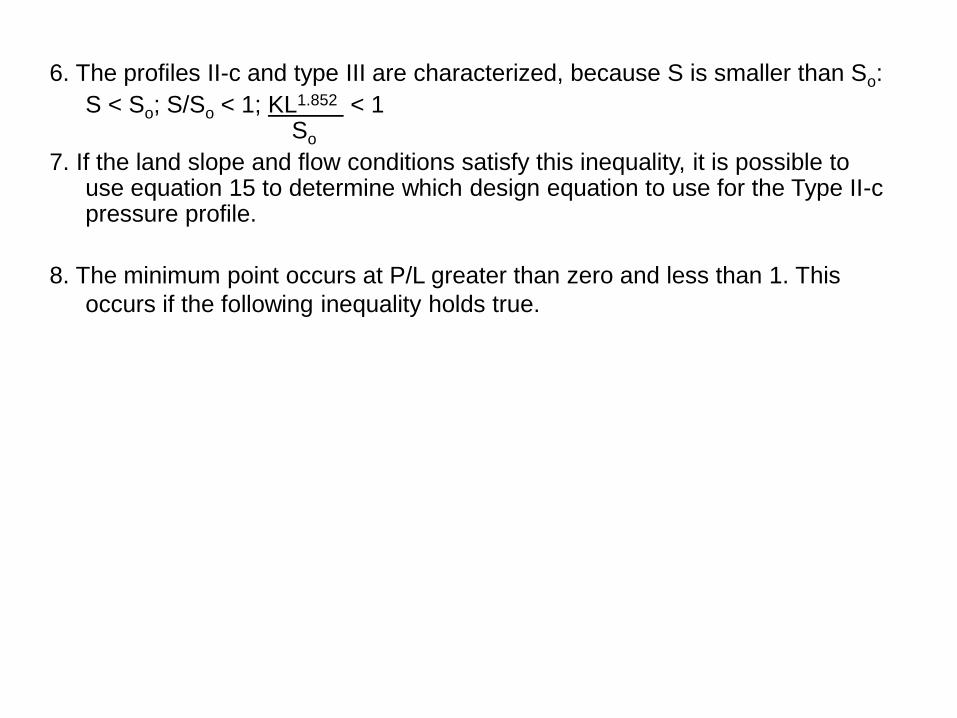
6. The profiles II-c and type III are characterized, because S is smaller than So:

S < So; S/So < 1; KL1.852 < 1 So

7. If the land slope and flow conditions satisfy this inequality, it is possible to use equation 15 to determine which design equation to use for the Type II-c pressure profile.

8. The minimum point occurs at P/L greater than zero and less than 1. This

occurs if the following inequality holds true.

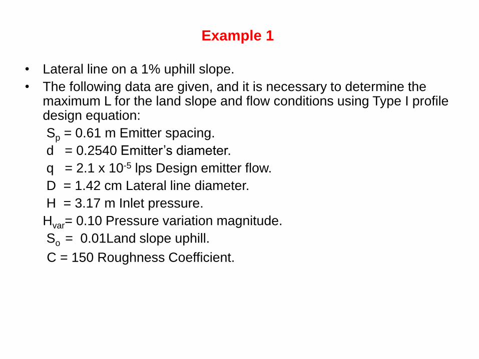
• Lateral line on a 1% uphill slope.

• The following data are given, and it is necessary to determine the maximum L for the land slope and flow conditions using Type I profile design equation:

Sp = 0.61 m Emitter spacing.

d = 0.2540 Emitter’s diameter.

q = 2.1 x 10-5 lps Design emitter flow.

D = 1.42 cm Lateral line diameter.

H = 3.17 m Inlet pressure.

Hvar= 0.10 Pressure variation magnitude.

So = 0.01Land slope uphill.

C = 150 Roughness Coefficient.

Example 1

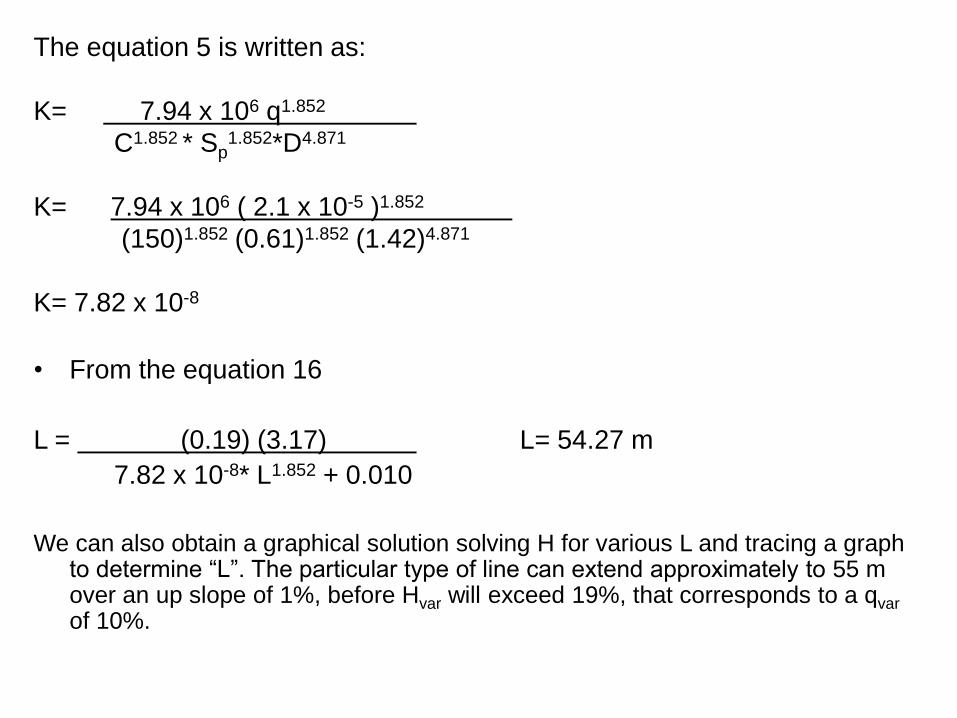
The equation 5 is written as:

K= 7.94 x 106 q1.852

C1.852 * Sp1.852*D4.871

K= 7.94 x 106 ( 2.1 x 10-5 )1.852

(150)1.852 (0.61)1.852 (1.42)4.871

K= 7.82 x 10-8

• From the equation 16

L = (0.19) (3.17) L= 54.27 m

7.82 x 10-8* L1.852 + 0.010

We can also obtain a graphical solution solving H for various L and tracing a graph to determine “L”. The particular type of line can extend approximately to 55 m over an up slope of 1%, before Hvar will exceed 19%, that corresponds to a qvar of 10%.

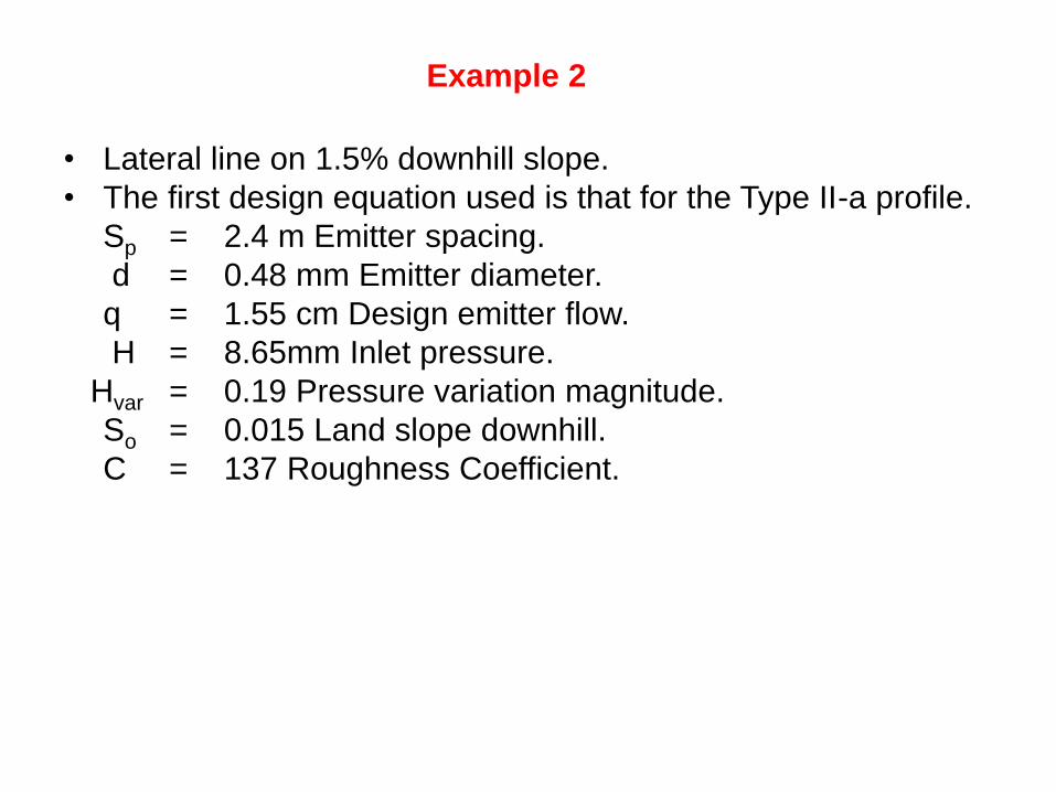
Example 2

• Lateral line on 1.5% downhill slope.

• The first design equation used is that for the Type II-a profile.

Sp = 2.4 m Emitter spacing.

d = 0.48 mm Emitter diameter.

q = 1.55 cm Design emitter flow.

H = 8.65mm Inlet pressure.

Hvar = 0.19 Pressure variation magnitude.

So = 0.015 Land slope downhill.

C = 137 Roughness Coefficient.

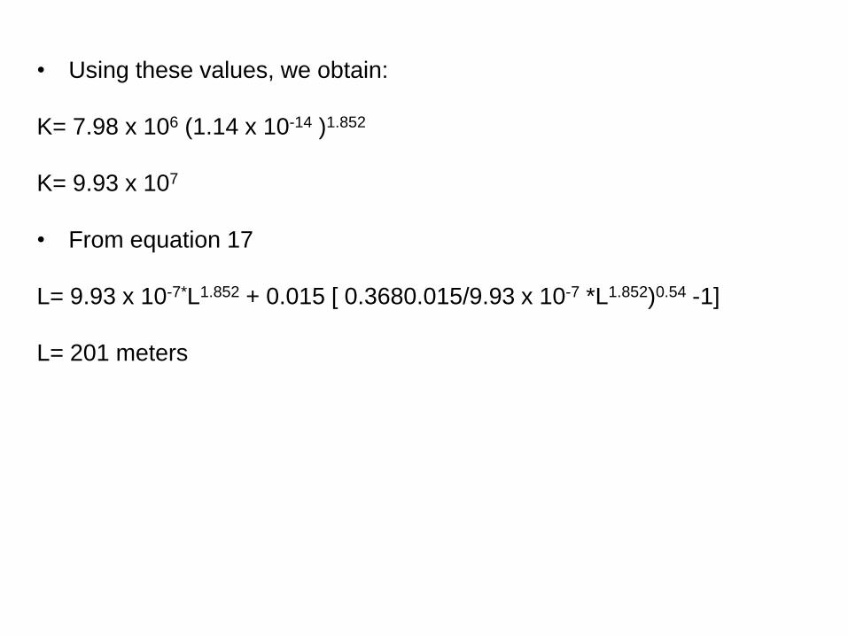
• Using these values, we obtain:

K= 7.98 x 106 (1.14 x 10-14 )1.852

K= 9.93 x 107

• From equation 17

L= 9.93 x 10-7*L1.852 + 0.015 [ 0.3680.015/9.93 x 10-7 *L1.852)0.54 -1]

L= 201 meters

Sprinkler Irrigation

Definition

• Pressurized irrigation through devices called sprinklers

• Sprinklers are usually located on pipes called laterals

• Water is discharged into the air and hopefully infiltrates near

where it lands

Types of Systems

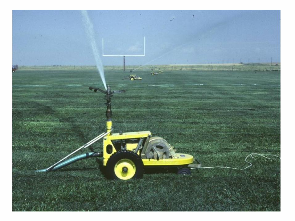
• Single sprinkler

– Only one sprinkler that is moved or automatically moves

• Examples:

– Single lawn sprinkler

– Large gun on a trailer that is moved or automatically moves (“traveler”)

• Often used for irregularly shaped areas

• Pressure and energy requirements can be high

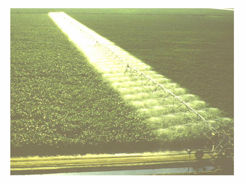
Solid Set

• Laterals are permanently placed (enough to irrigate the entire area)

• Laterals are usually buried, with risers or pop-up sprinklers

• Easily automated and popular for turf and some ag/hort

applications

• Capital investment can be high

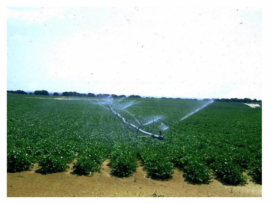
Periodically Moved Lateral

• Single lateral is moved and used in multiple locations

• Examples:

– Hand-move

– Tow-line/skid-tow (lateral is pulled across the field)

– Side-roll (lateral mounted on wheels that roll to move the lateral)

• Fairly high labor requirement

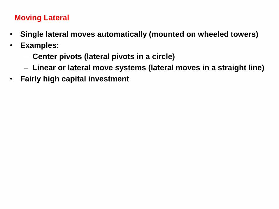
Moving Lateral

• Single lateral moves automatically (mounted on wheeled towers)

• Examples:

– Center pivots (lateral pivots in a circle)

– Linear or lateral move systems (lateral moves in a straight line)

• Fairly high capital investment

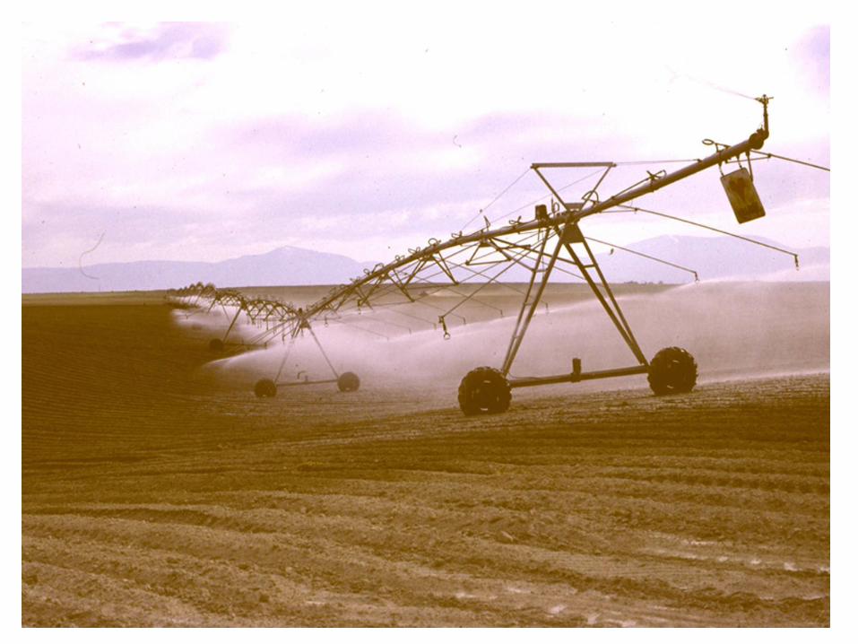
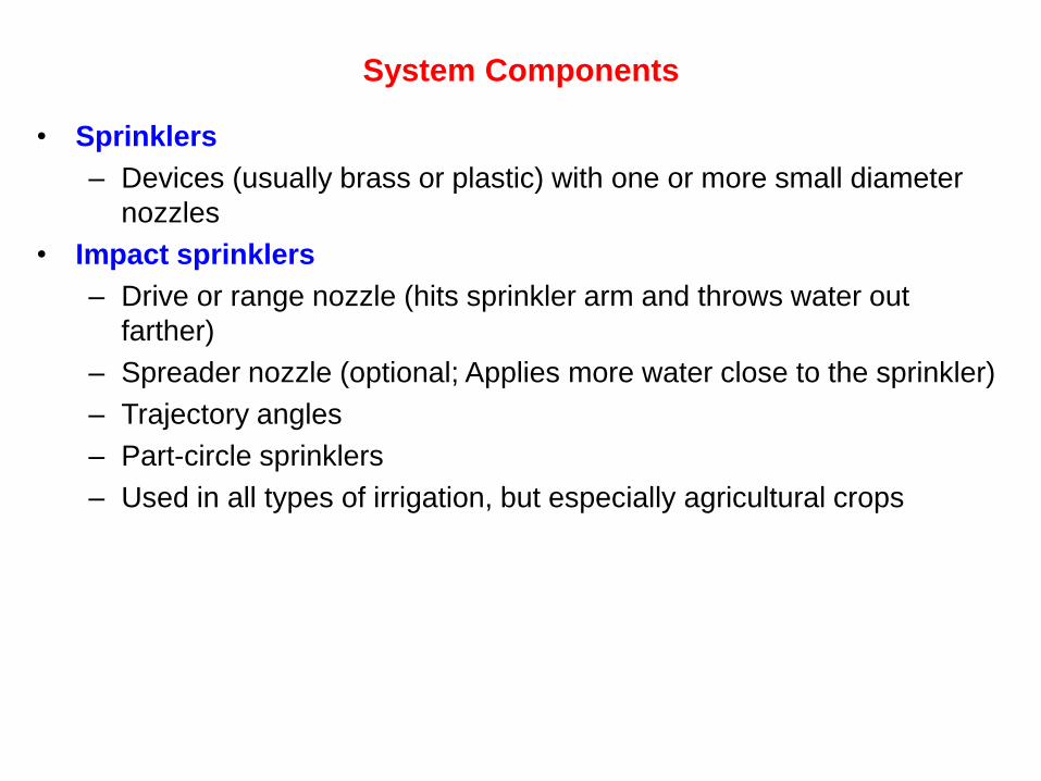
System Components

• Sprinklers

– Devices (usually brass or plastic) with one or more small diameter

nozzles

• Impact sprinklers

– Drive or range nozzle (hits sprinkler arm and throws water out

farther)

– Spreader nozzle (optional; Applies more water close to the sprinkler)

– Trajectory angles

– Part-circle sprinklers

– Used in all types of irrigation, but especially agricultural crops

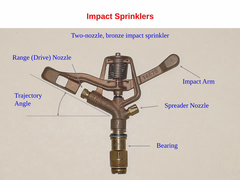
Impact Sprinklers

Impact Arm

Spreader Nozzle

Range (Drive) Nozzle

Bearing

Two-nozzle, bronze impact sprinkler

Trajectory

Angle

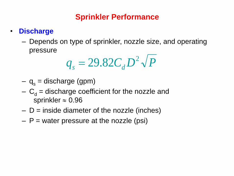
Sprinkler Performance

• Discharge

– Depends on type of sprinkler, nozzle size, and operating

pressure

– qs = discharge (gpm)

– Cd = discharge coefficient for the nozzle and

sprinkler 0.96

– D = inside diameter of the nozzle (inches)

– P = water pressure at the nozzle (psi)

PDCq ds

282.29

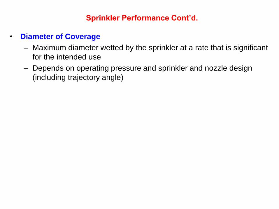
• Diameter of Coverage

– Maximum diameter wetted by the sprinkler at a rate that is significant

for the intended use

– Depends on operating pressure and sprinkler and nozzle design

(including trajectory angle)

Sprinkler Performance Cont’d.

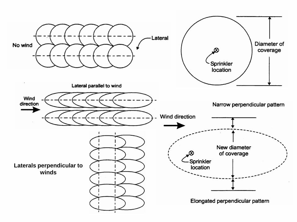
Laterals perpendicular to

winds

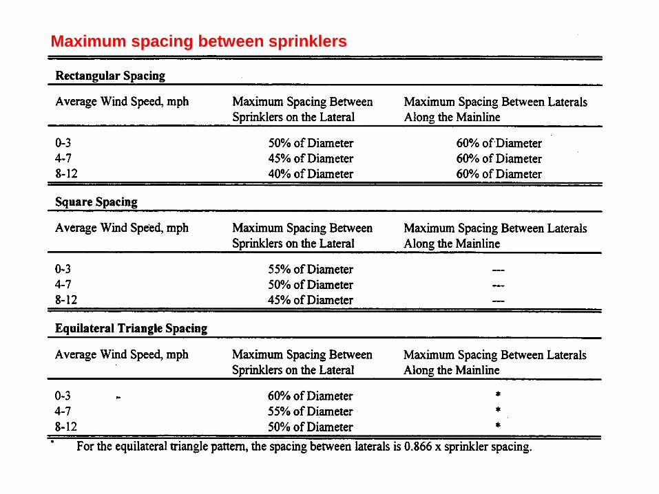
Maximum spacing between sprinklers

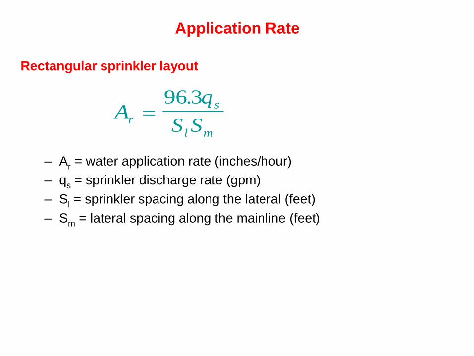
Rectangular sprinkler layout

– Ar = water application rate (inches/hour)

– qs = sprinkler discharge rate (gpm)

– Sl = sprinkler spacing along the lateral (feet)

– Sm = lateral spacing along the mainline (feet)

Aq

S Sr

s

l m

96 3.

Application Rate

Application Rate & Soil Infiltration Rate