lecture 5 – parallel programming patterns - map parallel programming patterns overview and map...

Lecture 5 – Parallel Programming Patterns - Map

Parallel Programming PatternsOverview and Map Pattern

Parallel Computing

CIS 410/510

Department of Computer and Information Science


Outline

• Parallel programming models• Dependencies• Structured programming patterns overview

– Serial / parallel control flow patterns– Serial / parallel data management patterns

• Map pattern– Optimizations

• sequences of Maps• code Fusion• cache Fusion

– Related Patterns– Example: Scaled Vector Addition (SAXPY)

2Introduction to Parallel Computing, University of Oregon, IPCC


Parallel Models 101

• Sequential models – von Neumann (RAM) model

• Parallel model– A parallel computer is simple a collection

of processors interconnected in some manner to coordinate activities and exchange data

– Models that can be used as general frameworks for describing and analyzing parallel algorithms• Simplicity: description, analysis, architecture independence• Implementability: able to be realized, reflect performance

• Three common parallel models– Directed acyclic graphs, shared-memory, network

Memory(RAM)

processor



Directed Acyclic Graphs (DAG)

• Captures data flow parallelism• Nodes represent operations to be performed

– Inputs are nodes with no incoming arcs– Output are nodes with no outgoing arcs– Think of nodes as tasks

• Arcs are paths for flow of data results• DAG represents the operations of the algorithm

and implies precedent constraints on their order

for (i=1; i<100; i++)

a[i] = a[i-1] + 100;a[0] a[1] a[99]…


Lecture 5 – Parallel Programming Patterns - Map 5

Shared Memory Model

• Parallel extension of RAM model (PRAM)– Memory size is infinite– Number of processors in unbounded– Processors communicate via the memory– Every processor accesses any memory

location in 1 cycle– Synchronous

• All processors execute same algorithm synchronously– READ phase– COMPUTE phase– WRITE phase

• Some subset of the processors can stay idle

– Asynchronous

SharedMemory

P3

PN

P1

P2

.

.

.

Introduction to Parallel Computing, University of Oregon, IPCC


Network Model

• G = (N,E)– N are processing nodes– E are bidirectional communication links

• Each processor has its own memory• No shared memory is available• Network operation may be synchronous or

asynchronous• Requires communication primitives

– Send (X, i)– Receive (Y, j)

• Captures message passing model for algorithm design

P31

PN1

P11

P21

.

.

.

P32

PN2

P12

P22

.

.

.

P3N

PNN

P1N

P2N

.

.

.



Parallelism

• Ability to execute different parts of a computation concurrently on different machines

• Why do you want parallelism?– Shorter running time or handling more work

• What is being parallelized?– Task: instruction, statement, procedure, …– Data: data flow, size, replication– Parallelism granularity

• Coarse-grain versus fine-grainded

• Thinking about parallelism• Evaluation



Why is parallel programming important?

• Parallel programming has matured– Standard programming models– Common machine architectures– Programmer can focus on computation and use suitable

programming model for implementation• Increase portability between models and architectures• Reasonable hope of portability across platforms• Problem

– Performance optimization is still platform-dependent– Performance portability is a problem– Parallel programming methods are still evolving



Parallel Algorithm Recipe to solve a problem “in parallel” on multiple

processing elements Standard steps for constructing a parallel algorithm

❍ Identify work that can be performed concurrently❍ Partition the concurrent work on separate processors❍ Properly manage input, output, and intermediate data❍ Coordinate data accesses and work to satisfy

dependencies Which are hard to do?



Parallelism Views

• Where can we find parallelism?• Program (task) view

– Statement level• Between program statements• Which statements can be executed at the same time?

– Block level / Loop level / Routine level / Process level• Larger-grained program statements

• Data view– How is data operated on?– Where does data reside?

• Resource view10Introduction to Parallel Computing, University of Oregon, IPCC


Parallelism, Correctness, and Dependence

• Parallel execution, from any point of view, will be constrained by the sequence of operations needed to be performed for a correct result

• Parallel execution must address control, data, and system dependences

• A dependency arises when one operation depends on an earlier operation to complete and produce a result before this later operation can be performed

• We extend this notion of dependency to resources since some operations may depend on certain resources– For example, due to where data is located



Executing Two Statements in Parallel

• Want to execute two statements in parallel• On one processor:

Statement 1;

Statement 2;• On two processors:

Processor 1: Processor 2:

Statement 1; Statement 2;

• Fundamental (concurrent) execution assumption– Processors execute independent of each other– No assumptions made about speed of processor execution



Sequential Consistency in Parallel Execution

• Case 1:Processor 1: Processor 2:

statement 1;

statement 2;• Case 2:

Processor 1: Processor 2:

statement 2;

statement 1;• Sequential consistency

– Statements execution does not interfere with each other– Computation results are the same (independent of order)

time

time



Independent versus Dependent

• In other words the execution of statement1;

statement2;

must be equivalent to

statement2;

statement1;

• Their order of execution must not matter!• If true, the statements are independent of each other• Two statements are dependent when the order of their

execution affects the computation outcome14Introduction to Parallel Computing, University of Oregon, IPCC


Examples

• Example 1S1: a=1;S2: b=1;

• Example 2S1: a=1;S2: b=a;

• Example 3S1: a=f(x);S2: a=b;

• Example 4S1: a=b;S2: b=1;

Statements are independent

Dependent (true (flow) dependence) Second is dependent on first Can you remove dependency?

Dependent (output dependence) Second is dependent on first Can you remove dependency? How?

Dependent (anti-dependence) First is dependent on second Can you remove dependency? How?



True Dependence and Anti-Dependence

• Given statements S1 and S2, S1;

S2;

• S2 has a true (flow) dependence on S1 if and only if

S2 reads a value written by S1

• S2 has a anti-dependence on S1 if and only if

S2 writes a value read by S1

X =

= X

...

= X

X =

... -1



Output Dependence

• Given statements S1 and S2, S1;

S2;• S2 has an output dependence on S1

if and only if

S2 writes a variable written by S1

• Anti- and output dependences are “name” dependencies– Are they “true” dependences?

• How can you get rid of output dependences?– Are there cases where you can not?

X =

X =

... 0



Statement Dependency Graphs

• Can use graphs to show dependence relationships• Example

S1: a=1;

S2: b=a;

S3: a=b+1;

S4: c=a;

• S2 S3 : S3 is flow-dependent on S2

• S1 0 S3 : S3 is output-dependent on S1

• S2 -1 S3 : S3 is anti-dependent on S2

S1

S2

S3

S4

flow

antioutput



When can two statements execute in parallel?

• Statements S1 and S2 can execute in parallel if and only if there are no dependences between S1 and S2– True dependences– Anti-dependences– Output dependences

• Some dependences can be remove by modifying the program– Rearranging statements– Eliminating statements



How do you compute dependence?

• Data dependence relations can be found by comparing the IN and OUT sets of each node

• The IN and OUT sets of a statement S are defined as:– IN(S) : set of memory locations (variables) that may be

used in S– OUT(S) : set of memory locations (variables) that may

be modified by S• Note that these sets include all memory locations

that may be fetched or modified• As such, the sets can be conservatively large



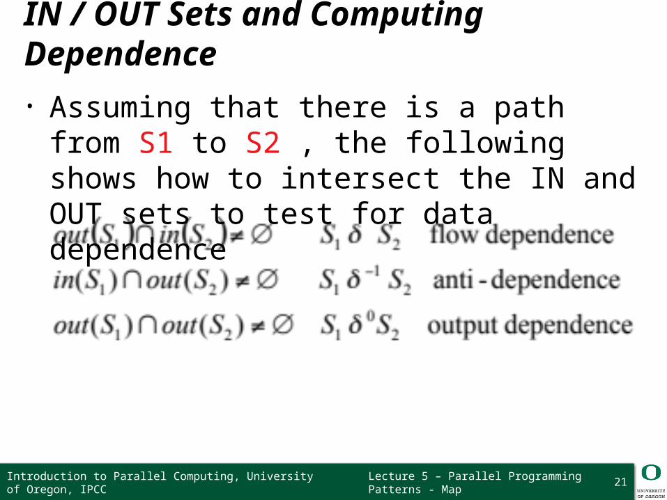
IN / OUT Sets and Computing Dependence

• Assuming that there is a path from S1 to S2 , the following shows how to intersect the IN and OUT sets to test for data dependence



Loop-Level Parallelism

• Significant parallelism can be identified within loops

for (i=0; i<100; i++) S1: a[i] = i;

• Dependencies? What about i, the loop index?• DOALL loop (a.k.a. foreach loop)

– All iterations are independent of each other– All statements be executed in parallel at the same time

• Is this really true?

for (i=0; i<100; i++) { S1: a[i] = i; S2: b[i] = 2*i;}



Iteration Space

• Unroll loop into separate statements / iterations• Show dependences between iterations

for (i=0; i<100; i++)

S1: a[i] = i;

S10

S20

for (i=0; i<100; i++) {

S1: a[i] = i;

S2: b[i] = 2*i;

}

S11

S21

S199

S299

S10 S11 S199… …



Multi-Loop Parallelism

• Significant parallelism can be identified between loops

for (i=0; i<100; i++) a[i] = i;

for (i=0; i<100; i++) b[i] = i;

• Dependencies?• How much parallelism is available?• Given 4 processors, how much parallelism is possible?• What parallelism is achievable with 50 processors?

a[0] a[1] a[99]…

b[0] b[1] b[99]…



Loops with Dependencies

Case 1:

for (i=1; i<100; i++)

a[i] = a[i-1] + 100;

• Dependencies?– What type?

• Is the Case 1 loop parallelizable?• Is the Case 2 loop parallelizable?

Case 2:

for (i=5; i<100; i++)

a[i-5] = a[i] + 100;

a[0] a[1] a[99]… a[0] a[5] a[10] …

a[1] a[6] a[11] …

a[2] a[7] a[12] …

a[3] a[8] a[13] …

a[4] a[9] a[14] …



Another Loop Example

for (i=1; i<100; i++)

a[i] = f(a[i-1]);

• Dependencies?– What type?

• Loop iterations are not parallelizable– Why not?



Loop Dependencies

• A loop-carried dependence is a dependence that is present only if the statements are part of the execution of a loop (i.e., between two statements instances in two different iterations of a loop)

• Otherwise, it is loop-independent, including between two statements instances in the same loop iteration

• Loop-carried dependences can prevent loop iteration parallelization

• The dependence is lexically forward if the source comes before the target or lexically backward otherwise– Unroll the loop to see



Loop Dependence Example

for (i=0; i<100; i++)

a[i+10] = f(a[i]);

• Dependencies?– Between a[10], a[20], …– Between a[11], a[21], …

• Some parallel execution is possible– How much?



Dependences Between Iterations

for (i=1; i<100; i++) {

S1: a[i] = …;

S2: … = a[i-1];

}

• Dependencies?– Between a[i] and a[i-1]

• Is parallelism possible?– Statements can be executed in “pipeline” manner

i1 2 3 4 5 6

S1

S2

…



Another Loop Dependence Example

for (i=0; i<100; i++)

for (j=1; j<100; j++)

a[i][j] = f(a[i][j-1]);

• Dependencies?– Loop-independent dependence on i– Loop-carried dependence on j

• Which loop can be parallelized?– Outer loop parallelizable– Inner loop cannot be parallelized



Still Another Loop Dependence Example

for (j=1; j<100; j++)

for (i=0; i<100; i++)

a[i][j] = f(a[i][j-1]);

• Dependencies?– Loop-independent dependence on i– Loop-carried dependence on j

• Which loop can be parallelized?– Inner loop parallelizable– Outer loop cannot be parallelized– Less desirable (why?)



Key Ideas for Dependency Analysis

• To execute in parallel:– Statement order must not matter– Statements must not have dependences

• Some dependences can be removed• Some dependences may not be obvious



Dependencies and Synchronization

• How is parallelism achieved when have dependencies?– Think about concurrency– Some parts of the execution are independent– Some parts of the execution are dependent

• Must control ordering of events on different processors (cores)– Dependencies pose constraints on parallel event ordering– Partial ordering of execution action

• Use synchronization mechanisms– Need for concurrent execution too– Maintains partial order



Parallel Patterns

• Parallel Patterns: A recurring combination of task distribution and data access that solves a specific problem in parallel algorithm design.

• Patterns provide us with a “vocabulary” for algorithm design

• It can be useful to compare parallel patterns with serial patterns

• Patterns are universal – they can be used in any parallel programming system



Parallel Patterns

• Nesting Pattern• Serial / Parallel Control Patterns• Serial / Parallel Data Management Patterns• Other Patterns• Programming Model Support for Patterns



Nesting Pattern

• Nesting is the ability to hierarchically compose patterns

• This pattern appears in both serial and parallel algorithms

• “Pattern diagrams” are used to visually show the pattern idea where each “task block” is a location of general code in an algorithm

• Each “task block” can in turn be another pattern in the nesting pattern



Nesting Pattern

37

Nesting Pattern: A compositional pattern. Nesting allows other patterns to be composed in a hierarchy so that any task block in the above diagram can be replaced with a pattern with the same input/output and dependencies.



Serial Control Patterns

• Structured serial programming is based on these patterns: sequence, selection, iteration, and recursion

• The nesting pattern can also be used to hierarchically compose these four patterns

• Though you should be familiar with these, it’s extra important to understand these patterns when parallelizing serial algorithms based on these patterns



Serial Control Patterns: Sequence

• Sequence: Ordered list of tasks that are executed in a specific order

• Assumption – program text ordering will be followed (obvious, but this will be important when parallelized)



Serial Control Patterns: Selection

• Selection: condition c is first evaluated. Either task a or b is executed depending on the true or false result of c.

• Assumptions – a and b are never executed before c, and only a or b is executed - never both



Serial Control Patterns: Iteration

• Iteration: a condition c is evaluated. If true, a is evaluated, and then c is evaluated again. This repeats until c is false.

• Complication when parallelizing: potential for dependencies to exist between previous iterations



Serial Control Patterns: Recursion

• Recursion: dynamic form of nesting allowing functions to call themselves

• Tail recursion is a special recursion that can be converted into iteration – important for functional languages



Parallel Control Patterns

• Parallel control patterns extend serial control patterns

• Each parallel control pattern is related to at least one serial control pattern, but relaxes assumptions of serial control patterns

• Parallel control patterns: fork-join, map, stencil, reduction, scan, recurrence



Parallel Control Patterns: Fork-Join

• Fork-join: allows control flow to fork into multiple parallel flows, then rejoin later

• Cilk Plus implements this with spawn and sync– The call tree is a parallel call tree and functions are

spawned instead of called– Functions that spawn another function call will continue

to execute– Caller syncs with the spawned function to join the two

• A “join” is different than a “barrier– Sync – only one thread continues– Barrier – all threads continue



Parallel Control Patterns: Map• Map: performs a function over every element of a collection• Map replicates a serial iteration pattern where each iteration is

independent of the others, the number of iterations is known in advance, and computation only depends on the iteration count and data from the input collection

• The replicated function is referred to as an “elemental function”

45

Input

Elemental Function

Output



Parallel Control Patterns: Stencil

• Stencil: Elemental function accesses a set of “neighbors”, stencil is a generalization of map

• Often combined with iteration – used with iterative solvers or to evolve a system through time

46

Boundary conditions must be handled carefully in the stencil pattern

See stencil lecture…



Parallel Control Patterns: Reduction

• Reduction: Combines every element in a collection using an associative “combiner function”

• Because of the associativity of the combiner function, different orderings of the reduction are possible

• Examples of combiner functions: addition, multiplication, maximum, minimum, and Boolean AND, OR, and XOR



Parallel Control Patterns: Reduction

48

Serial Reduction Parallel Reduction



Parallel Control Patterns: Scan

• Scan: computes all partial reduction of a collection• For every output in a collection, a reduction of the

input up to that point is computed• If the function being used is associative, the scan

can be parallelized• Parallelizing a scan is not obvious at first, because

of dependencies to previous iterations in the serial loop

• A parallel scan will require more operations than a serial version



Parallel Control Patterns: Scan

50

Serial Scan Parallel Scan



Parallel Control Patterns: Recurrence

• Recurrence: More complex version of map, where the loop iterations can depend on one another

• Similar to map, but elements can use outputs of adjacent elements as inputs

• For a recurrence to be computable, there must be a serial ordering of the recurrence elements so that elements can be computed using previously computed outputs



Serial Data Management Patterns

• Serial programs can manage data in many ways• Data management deals with how data is

allocated, shared, read, written, and copied• Serial Data Management Patterns: random read

and write, stack allocation, heap allocation, objects



Serial Data Management Patterns: random read and write

• Memory locations indexed with addresses• Pointers are typically used to refer to memory

addresses• Aliasing (uncertainty of two pointers referring to

the same object) can cause problems when serial code is parallelized



Serial Data Management Patterns: Stack Allocation

• Stack allocation is useful for dynamically allocating data in LIFO manner

• Efficient – arbitrary amount of data can be allocated in constant time

• Stack allocation also preserves locality• When parallelized, typically each thread will get

its own stack so thread locality is preserved



Serial Data Management Patterns: Heap Allocation

• Heap allocation is useful when data cannot be allocated in a LIFO fashion

• But, heap allocation is slower and more complex than stack allocation

• A parallelized heap allocator should be used when dynamically allocating memory in parallel– This type of allocator will keep separate pools for each

parallel worker



Serial Data Management Patterns: Objects

• Objects are language constructs to associate data with code to manipulate and manage that data

• Objects can have member functions, and they also are considered members of a class of objects

• Parallel programming models will generalize objects in various ways



Parallel Data Management Patterns

• To avoid things like race conditions, it is critically important to know when data is, and isn’t, potentially shared by multiple parallel workers

• Some parallel data management patterns help us with data locality

• Parallel data management patterns: pack, pipeline, geometric decomposition, gather, and scatter



Parallel Data Management Patterns: Pack

• Pack is used eliminate unused space in a collection• Elements marked false are discarded, the remaining

elements are placed in a contiguous sequence in the same order

• Useful when used with

map• Unpack is the inverse

and is used to place

elements back in their

original locations58Introduction to Parallel Computing, University of Oregon, IPCC


Parallel Data Management Patterns: Pipeline

• Pipeline connects tasks in a producer-consumer manner

• A linear pipeline is the basic pattern idea, but a pipeline in a DAG is also possible

• Pipelines are most useful when used with other patterns as they can multiply available parallelism



Parallel Data Management Patterns: Geometric Decomposition

• Geometric Decomposition – arranges data into subcollections

• Overlapping and non-overlapping decompositions are possible

• This pattern doesn’t necessarily move data, it just gives us another view of it



Parallel Data Management Patterns: Gather

• Gather reads a collection of data given a collection of indices

• Think of a combination of map and random serial reads

• The output collection shares the same type as the input collection, but it share the same shape as the indices collection



Parallel Data Management Patterns: Scatter

• Scatter is the inverse of gather• A set of input and indices is required, but each

element of the input is written to the output at the given index instead of read from the input at the given index

• Race conditions can occur when we have two writes to the same location!



Other Parallel Patterns

• Superscalar Sequences: write a sequence of tasks, ordered only by dependencies

• Futures: similar to fork-join, but tasks do not need to be nested hierarchically

• Speculative Selection: general version of serial selection where the condition and both outcomes can all run in parallel

• Workpile: general map pattern where each instance of elemental function can generate more instances, adding to the “pile” of work



Other Parallel Patterns

• Search: finds some data in a collection that meets some criteria

• Segmentation: operations on subdivided, non-overlapping, non-uniformly sized partitions of 1D collections

• Expand: a combination of pack and map• Category Reduction: Given a collection of

elements each with a label, find all elements with same label and reduce them



Programming Model Support for Patterns



Map Pattern - Overview Map Optimizations

❍ Sequences of Maps❍ Code Fusion❍ Cache Fusion

Related Patterns Example Implementation: Scaled Vector Addition

(SAXPY)❍ Problem Description❍ Various Implementations



Mapping “Do the same thing many times”

foreach i in foo:do something

Well-known higher order function in languages like ML, Haskell, Scala

map: applies a function each element in a list and

returns a list of results



Example MapsAdd 1 to every item in an array Double every item in an array

0 4 5 3 1 0

0 1 2 3 4 5

1 5 6 4 2 1

3 7 0 1 4 0

6 14 0 2 8 0

0 1 2 3 4 5

Key Point: An operation is a map if it can be applied to each element without knowledge of neighbors.



Key Idea Map is a “foreach loop” where each iteration is

independent

71

Embarrassingly Parallel

Independence is a big win. We can run map completely in parallel. Significant speedups! More precisely: is O(1) plus implementation overhead that is O(log n)…so .



Sequential Map

for(int n=0; n< array.length; ++n){

process(array[n]);}

72

Tim

e



Parallel Map

parallel_for_each(x in array){

process(x);}

73

Tim

e



Comparing MapsSerial Map

74

Parallel Map



Comparing MapsSerial Map

75

Parallel Map

Speedup

The space here is speedup. With the parallel map, our program finished execution early, while the serial map is still running.



Independence The key to (embarrasing) parallelism is

independence

Modifying shared state breaks perfect independence Results of accidentally violating independence:

❍ non-determinism❍ data-races❍ undefined behavior❍ segfaults

76

Map function should be “pure” (or “pure-ish”) and should not modify shared states

Warning: No shared state!



Implementation and API OpenMP and CilkPlus contain a parallel for language

construct Map is a mode of use of parallel for TBB uses higher order functions with lambda

expressions/“funtors” Some languages (CilkPlus, Matlab, Fortran) provide

array notation which makes some maps more concise

77

A[:] = A[:]*5;is CilkPlus array notation for “multiply every element in A by 5”

Array Notation



Unary Maps

78

So far we have only dealt with mapping over a single collection…

Unary Maps



Map with 1 Input, 1 Output

x 3 7 0 1 4 0 0 4 5 3 1 0

0 1 2 3 4 5 6 7 8 9 10 11

6 14 0 2 8 0 0 8 10 6 2 0result

int oneToOne ( int x[11] ) {return x*2;

}



N-ary Maps

80

But, sometimes it makes sense to map over multiple collections at once…

N-ary Maps



Map with 2 Inputs, 1 Output

x 3 7 0 1 4 0 0 4 5 3 1 0

0 1 2 3 4 5 6 7 8 9 10 11

5 11 2 2 12 3 9 9 10 4 3 1result

y 2 4 2 1 8 3 9 5 5 1 2 1

int twoToOne ( int x[11], int y[11] ) {return x+y;

}



Optimization – Sequences of Maps Often several map

operations occur in sequence❍ Vector math consists of many

small operations such as additions and multiplications applied as maps

A naïve implementation may write each intermediate result to memory, wasting memory BW and likely overwhelming the cache



Optimization – Code Fusion Can sometimes

“fuse” together the operations to perform them at once

Adds arithmetic intensity, reduces memory/cache usage

Ideally, operations can be performed using registers alone



Optimization – Cache Fusion Sometimes

impractical to fuse together the map operations

Can instead break the work into blocks, giving each CPU one block at a time

Hopefully, operations use cache alone



Related Patterns

Three patterns related to map are discussed here:❍ Stencil❍ Workpile❍ Divide-and-Conquer

More detail presented in a later lecture



Stencil Each instance of the map function accesses

neighbors of its input, offset from its usual input Common in imaging and PDE solvers



Workpile Work items can be added to the map while it is in

progress, from inside map function instances Work grows and is consumed by the map Workpile pattern terminates when no more work is

available



Divide-and-Conquer Applies if a problem can

be divided into smaller subproblems recursively until a base case is reached that can be solved serially



Example: Scaled Vector Addition (SAXPY)

❍ Scales vector x by a and adds it to vector y❍ Result is stored in input vector y

Comes from the BLAS (Basic Linear Algebra Subprograms) library

Every element in vector x and vector y are independent



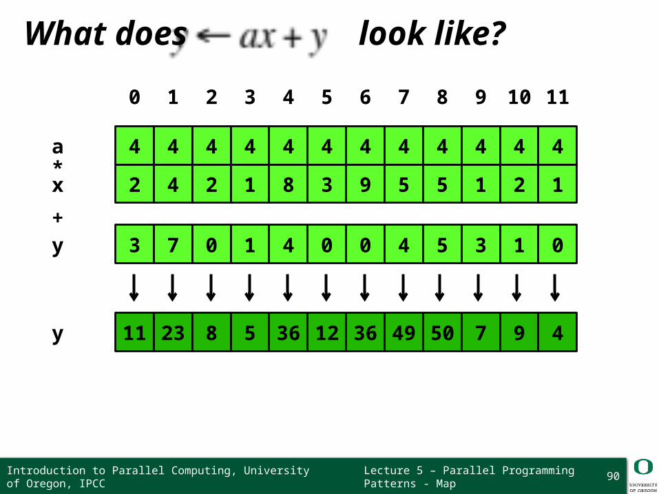
What does look like?

90

a 4 4 4 4 4 4 4 4 4 4 4 4

0 1 2 3 4 5 6 7 8 9 10 11

11 23 8 5 36 12 36 49 50 7 9 4y

y 3 7 0 1 4 0 0 4 5 3 1 0

x 2 4 2 1 8 3 9 5 5 1 2 1*

+



Visual:

91

a 4 4 4 4 4 4 4 4 4 4 4 4

0 1 2 3 4 5 6 7 8 9 10 11

11 23 8 5 36 12 36 49 50 7 9 4y

y 3 7 0 1 4 0 0 4 5 3 1 0

x 2 4 2 1 8 3 9 5 5 1 2 1*

+

Twelve processors used one for each element in the vector



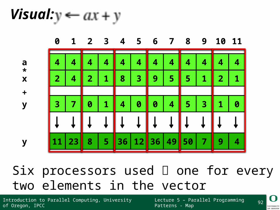
Visual:

92

a 4 4 4 4 4 4 4 4 4 4 4 4

0 1 2 3 4 5 6 7 8 9 10 11

11 23 8 5 36 12 36 49 50 7 9 4y

y 3 7 0 1 4 0 0 4 5 3 1 0

x 2 4 2 1 8 3 9 5 5 1 2 1*

+

Six processors used one for every two elements in the vector



Visual:

93

a 4 4 4 4 4 4 4 4 4 4 4 4

0 1 2 3 4 5 6 7 8 9 10 11

11 23 8 5 36 12 36 49 50 7 9 4y

y 3 7 0 1 4 0 0 4 5 3 1 0

x 2 4 2 1 8 3 9 5 5 1 2 1*

+

Two processors used one for every six elements in the vector



Serial SAXPY Implementation



TBB SAXPY Implementation



Cilk Plus SAXPY Implementation



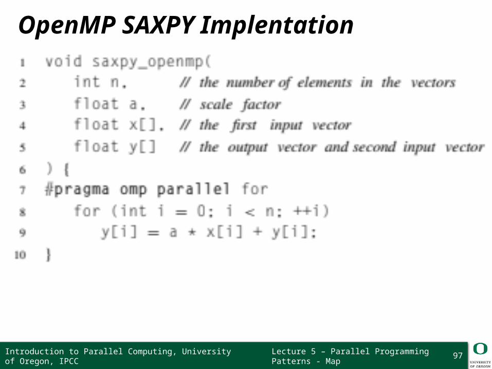
OpenMP SAXPY Implentation



OpenMP SAXPY Performance

98

Vector size = 500,000,000


lecture 5 – parallel programming patterns - map parallel programming patterns overview and map...

Documents

parallel algorithmssimplicity

flow of data resultsdag

university of oregon

outgoing arcsthink of

sequential models

department of computer

scaled vector addition

information science