34-1

Lecture 34

Fixed vs Random Effects

STAT 512

Spring 2011

Background Reading

KNNL: Chapter 25

34-2

Topic Overview

• Random vs. Fixed Effects

• Using Expected Mean Squares (EMS) to

obtain appropriate tests in a Random or

Mixed Effects Model

34-3

Fixed vs. Random Effects

• So far we have considered only fixed effect

models in which the levels of each factor

were fixed in advance of the experiment

and we were interested in differences in

response among those specific levels.

• A random effects model considers factors

for which the factor levels are meant to be

representative of a general population of

possible levels.

34-4

Fixed vs. Random Effects (2)

• For a random effect, we are interested in

whether that factor has a significant effect

in explaining the response, but only in a

general way.

• If we have both fixed and random effects,

we call it a “mixed effects model”.

• To include random effects in SAS, either use

the MIXED procedure, or use the GLM

procedure with a RANDOM statement.

34-5

Fixed vs. Random Effects (2)

• In some situations it is clear from the

experiment whether an effect is fixed or

random. However there are also situations

in which calling an effect fixed or random

depends on your point of view, and on

your interpretation and understanding. So

sometimes it is a personal choice. This

should become more clear with some

examples.

34-6

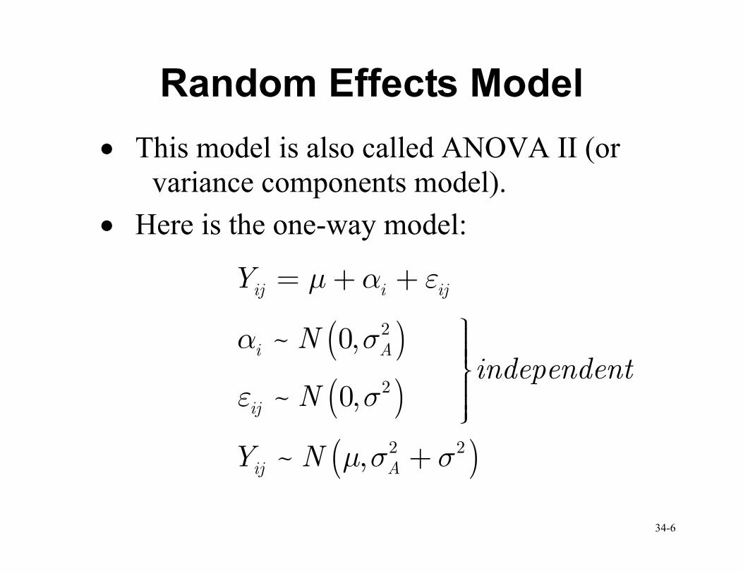
Random Effects Model

• This model is also called ANOVA II (or

variance components model).

• Here is the one-way model:

( )

( )

( )

2

2

2 2

~ 0,

~ 0,

~ ,

ij i ij

i A

ij

ij A

Y

Nindependent

N

Y N

µ α ε

α σ

ε σ

µ σ σ

= + +

+

34-7

Random Effects Model (2)

Now the cell means i iµ µ α= + are random

variables with a common mean. The question of

“are they all the same” can now be addressed by

considering whether the variance of their

distribution is zero. Of course, the estimated

means will likely be at least slightly different

from each other; the question is whether the

difference can be explained by error variance 2σ

alone.

34-8

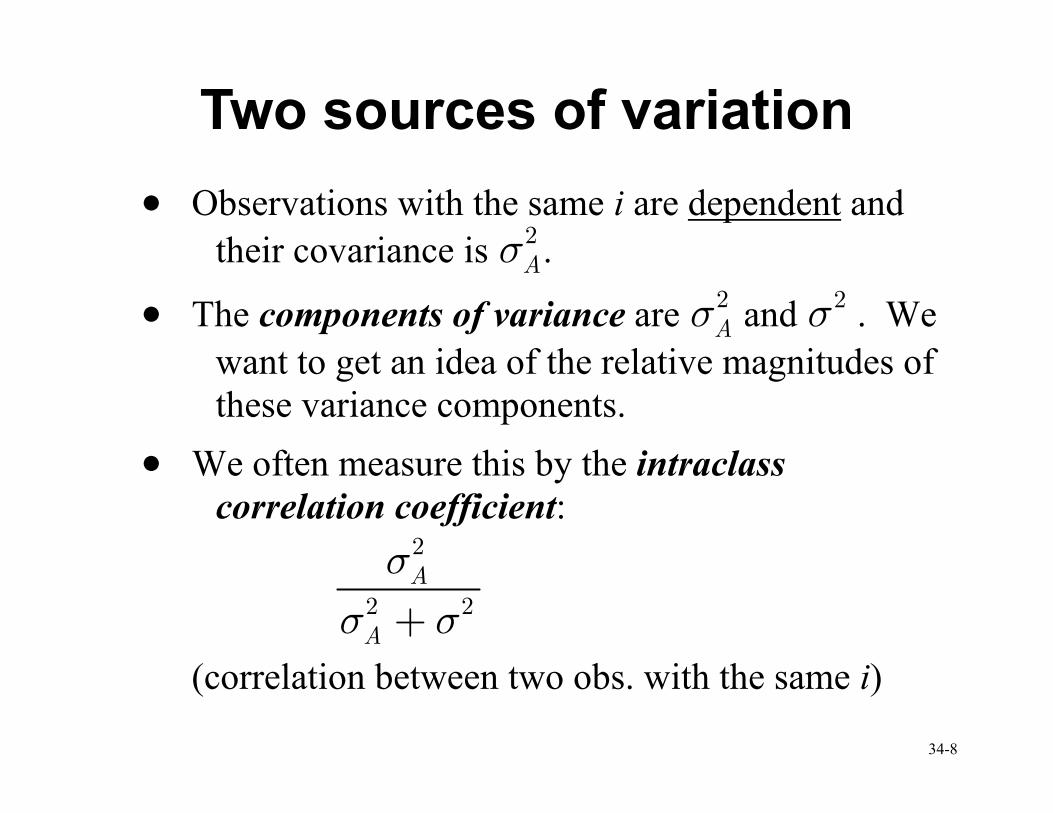
Two sources of variation

• Observations with the same i are dependent and

their covariance is 2Aσ .

• The components of variance are 2Aσ and

2σ . We

want to get an idea of the relative magnitudes of

these variance components.

• We often measure this by the intraclass

correlation coefficient:

2

2 2A

A

σ

σ σ+

(correlation between two obs. with the same i)

34-9

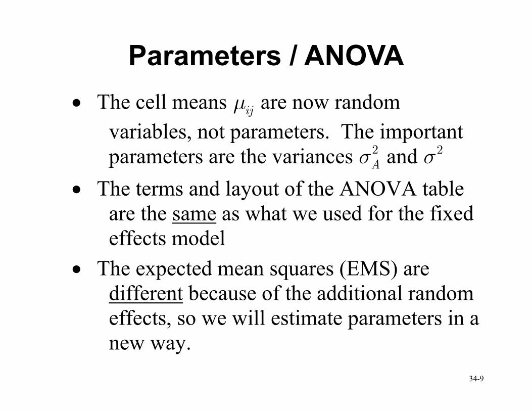
Parameters / ANOVA

• The cell means ijµ are now random

variables, not parameters. The important

parameters are the variances 2Aσ and 2σ

• The terms and layout of the ANOVA table

are the same as what we used for the fixed

effects model

• The expected mean squares (EMS) are

different because of the additional random

effects, so we will estimate parameters in a

new way.

34-10

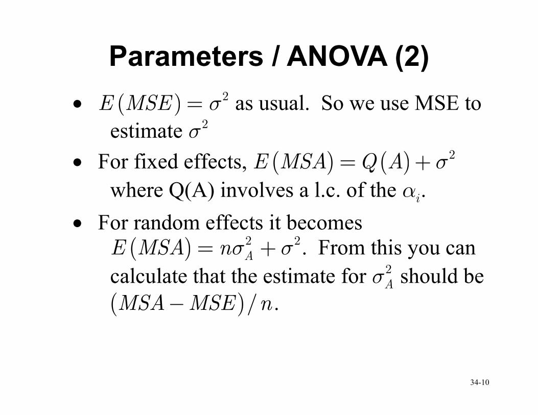
Parameters / ANOVA (2)

• ( ) 2E MSE σ= as usual. So we use MSE to

estimate 2σ

• For fixed effects, ( ) ( ) 2E MSA Q A σ= +

where Q(A) involves a l.c. of the iα .

• For random effects it becomes

( ) 2 2AE MSA nσ σ= + . From this you can

calculate that the estimate for 2Aσ should be

( )/MSA MSE n− .

34-11

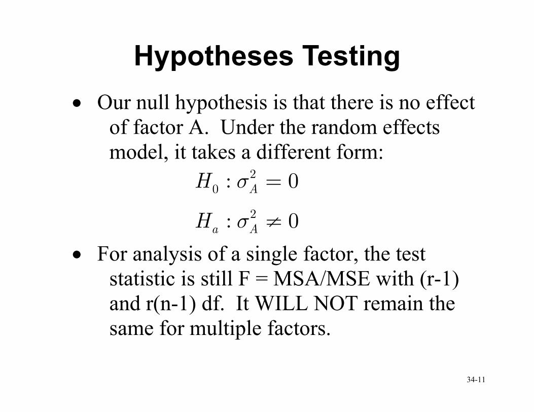
Hypotheses Testing

• Our null hypothesis is that there is no effect

of factor A. Under the random effects

model, it takes a different form:

20

2

: 0

: 0

A

a A

H

H

σ

σ

=

≠

• For analysis of a single factor, the test

statistic is still F = MSA/MSE with (r-1)

and r(n-1) df. It WILL NOT remain the

same for multiple factors.

34-12

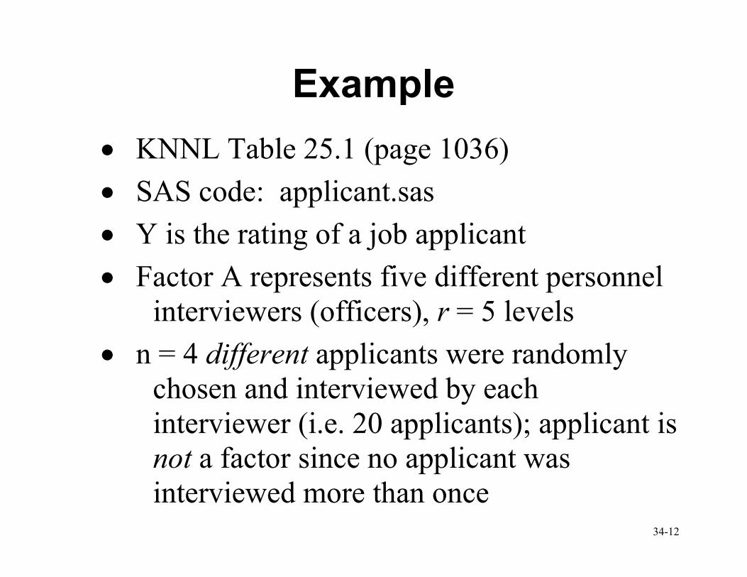
Example

• KNNL Table 25.1 (page 1036)

• SAS code: applicant.sas

• Y is the rating of a job applicant

• Factor A represents five different personnel

interviewers (officers), r = 5 levels

• n = 4 different applicants were randomly

chosen and interviewed by each

interviewer (i.e. 20 applicants); applicant is

not a factor since no applicant was

interviewed more than once

34-13

Example (2)

• The interviewers were selected at random

from the pool of interviewers and had

applicants randomly assigned.

• Here we are not so interested in the

differences between the five interviewers

that happened to be picked (i.e. does Joe

give higher ratings than Fred, is there a

difference between Ethel and Bob). Rather

we are interested in quantifying and

accounting for the effect of “interviewer” in

general.

34-14

Example (3)

• There are other interviewers in the

“population” and we want to make

inference about them too.

• Another way to say this is that with fixed

effects we are primarily interested in the

means of the factor levels (and differences

between them). With random effects, we

are primarily interested in their variances.

34-15

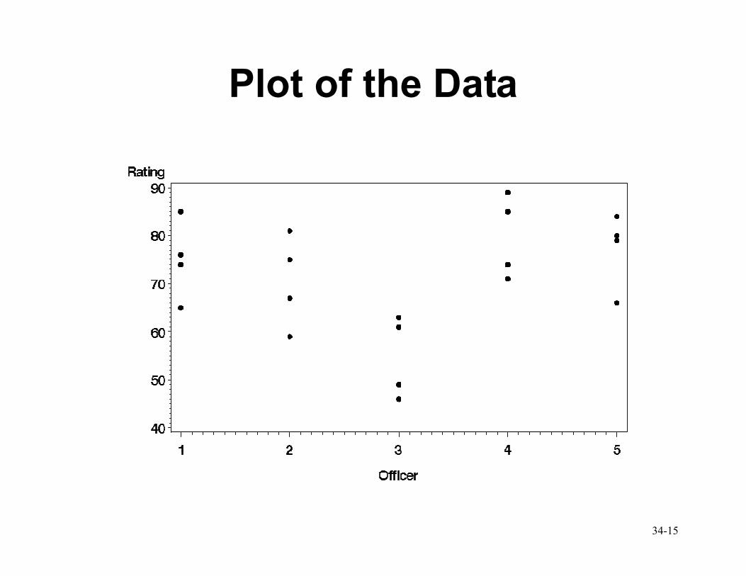
Plot of the Data

34-16

34-17

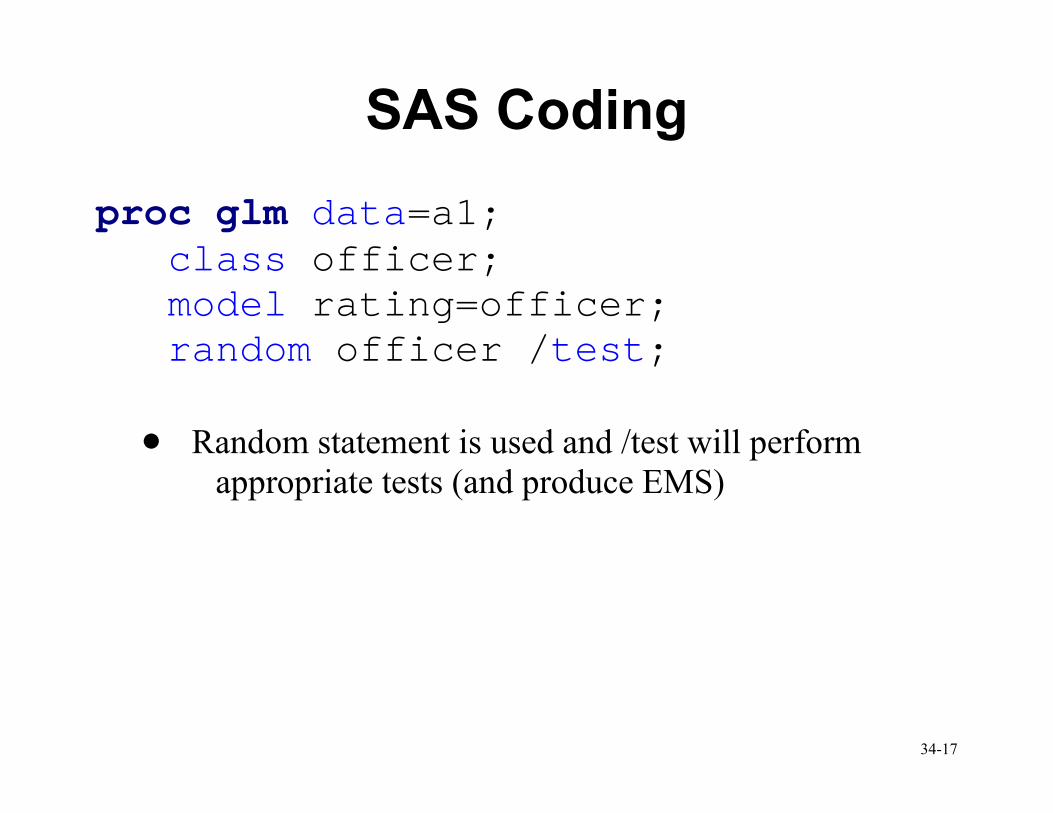
SAS Coding

proc glm data=a1; class officer; model rating=officer; random officer /test;

• Random statement is used and /test will perform

appropriate tests (and produce EMS)

34-18

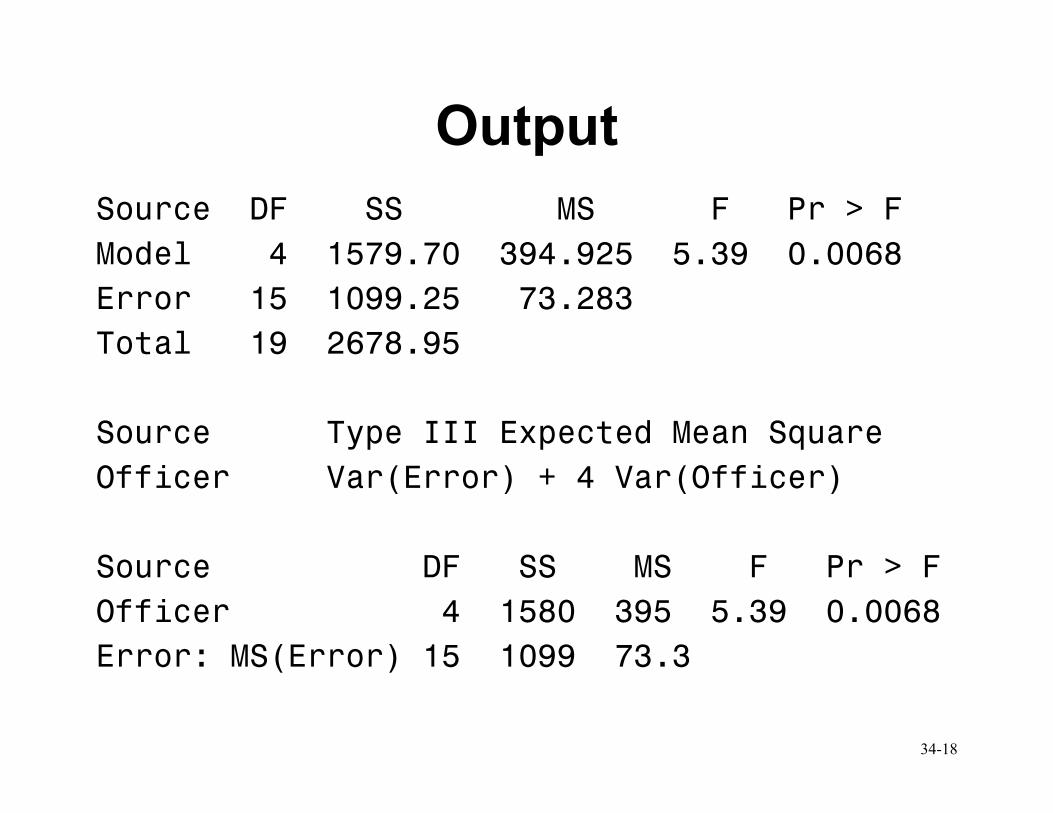
Output

Source DF SS MS F Pr > F

Model 4 1579.70 394.925 5.39 0.0068

Error 15 1099.25 73.283

Total 19 2678.95

Source Type III Expected Mean Square

Officer Var(Error) + 4 Var(Officer)

Source DF SS MS F Pr > F

Officer 4 1580 395 5.39 0.0068

Error: MS(Error) 15 1099 73.3

34-19

Output (2)

• SAS gives us the EMS (note n = 4

replicates): ( ) 2 24 AE MSA σ σ= +

• SAS provides the appropriate test for each

effect and tells you what “error term” is

being used in testing. Note for this

example it is as usual since there is only

one factor.

34-20

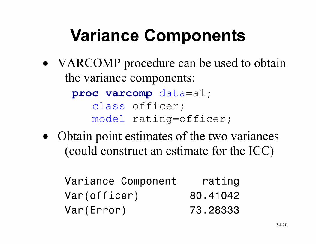
Variance Components

• VARCOMP procedure can be used to obtain

the variance components: proc varcomp data=a1; class officer; model rating=officer;

• Obtain point estimates of the two variances

(could construct an estimate for the ICC)

Variance Component rating

Var(officer) 80.41042

Var(Error) 73.28333

34-21

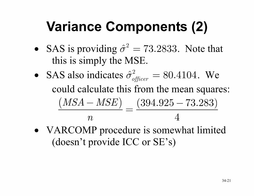
Variance Components (2)

• SAS is providing 2ˆ 73.2833σ = . Note that

this is simply the MSE.

• SAS also indicates 2ˆ 80.4104officerσ = . We

could calculate this from the mean squares:

( ) ( )394.925 73.283

4

MSA MSE

n

− −=

• VARCOMP procedure is somewhat limited

(doesn’t provide ICC or SE’s)

34-22

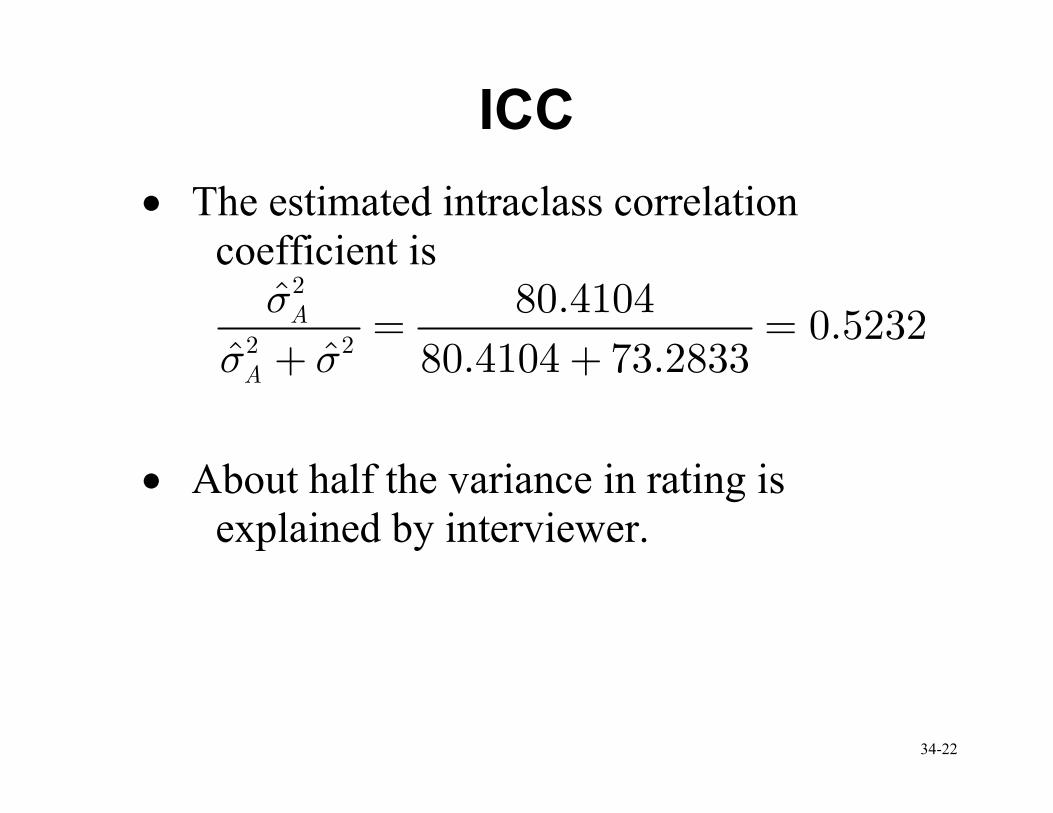
ICC

• The estimated intraclass correlation

coefficient is 2

2 2

ˆ 80.41040.5232

ˆ ˆ 80.4104 73.2833A

A

σ

σ σ= =

+ +

• About half the variance in rating is

explained by interviewer.

34-23

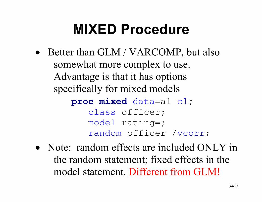
MIXED Procedure

• Better than GLM / VARCOMP, but also

somewhat more complex to use.

Advantage is that it has options

specifically for mixed models proc mixed data=a1 cl; class officer; model rating=; random officer /vcorr;

• Note: random effects are included ONLY in

the random statement; fixed effects in the

model statement. Different from GLM!

34-24

Mixed Procedure

• The cl option after data=a1 asks for the

confidence limits (on the variances).

• VCORR option provides the intraclass

correlation coefficient.

• Have to watch out for huge amounts of

output – in this case there were 5 pages –

we’ll just go through some of the pieces.

34-25

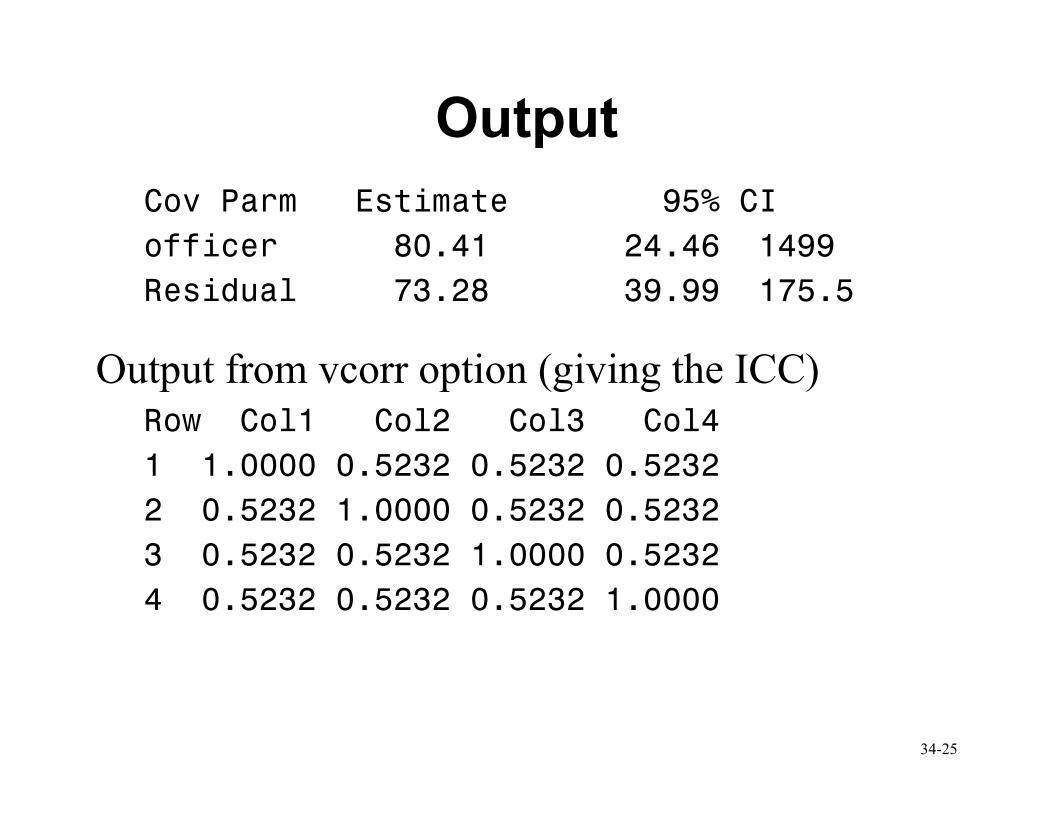
Output

Cov Parm Estimate 95% CI

officer 80.41 24.46 1499

Residual 73.28 39.99 175.5

Output from vcorr option (giving the ICC) Row Col1 Col2 Col3 Col4

1 1.0000 0.5232 0.5232 0.5232

2 0.5232 1.0000 0.5232 0.5232

3 0.5232 0.5232 1.0000 0.5232

4 0.5232 0.5232 0.5232 1.0000

34-26

Notes from Example

• Confidence intervals for variance components are

discussed in KNNL (pgs1041-1047)

• In this example, we would like the ICC to be

small, indicating that the variance due to the

interviewer is small relative to the variance due to

applicants. In many other examples, we may want

this quantity to be large.

• What we found is that there is a significant effect

of personnel officer (interviewer).

34-27

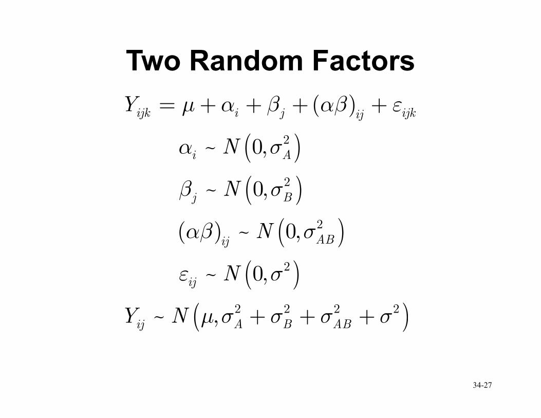
Two Random Factors

( )

( )

( )

( ) ( )

( )

( )

2

2

2

2

2 2 2 2

~ 0,

~ 0,

~ 0,

~ 0,

~ ,

ijk i j ijkij

i A

j B

ABij

ij

ij A B AB

Y

N

N

N

N

Y N

µ α β αβ ε

α σ

β σ

αβ σ

ε σ

µ σ σ σ σ

= + + + +

+ + +

34-28

Two Random Factors (2)

• Now the component 2µσ can be divided up

into three components – A, B, and AB.

• There are five parameters in this model: 2 2 2 2, , , ,A B ABµ σ σ σ σ .

• Again, the cell means are random variables,

not parameters!!!

34-29

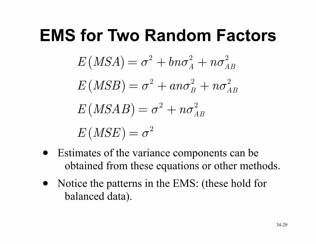
EMS for Two Random Factors

( )

( )

( )

( )

2 2 2

2 2 2

2 2

2

A AB

B AB

AB

E MSA bn n

E MSB an n

E MSAB n

E MSE

σ σ σ

σ σ σ

σ σ

σ

= + +

= + +

= +

=

• Estimates of the variance components can be

obtained from these equations or other methods.

• Notice the patterns in the EMS: (these hold for

balanced data).

34-30

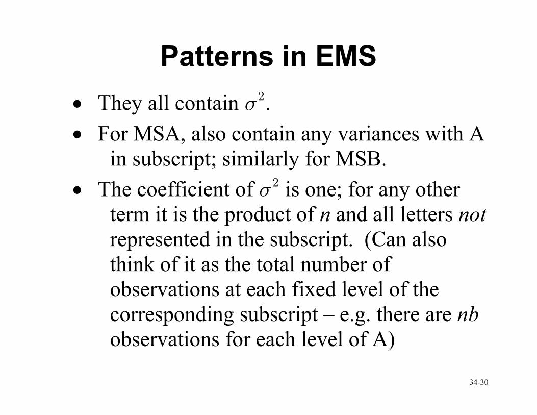
Patterns in EMS

• They all contain 2σ .

• For MSA, also contain any variances with A

in subscript; similarly for MSB.

• The coefficient of 2σ is one; for any other

term it is the product of n and all letters not

represented in the subscript. (Can also

think of it as the total number of

observations at each fixed level of the

corresponding subscript – e.g. there are nb

observations for each level of A)

34-31

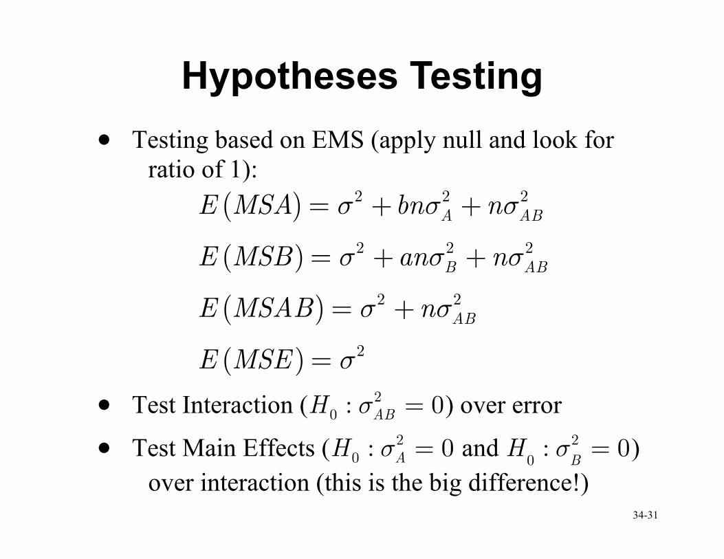
Hypotheses Testing

• Testing based on EMS (apply null and look for

ratio of 1):

( )

( )

( )

( )

2 2 2

2 2 2

2 2

2

A AB

B AB

AB

E MSA bn n

E MSB an n

E MSAB n

E MSE

σ σ σ

σ σ σ

σ σ

σ

= + +

= + +

= +

=

• Test Interaction ( 20 : 0ABH σ = ) over error

• Test Main Effects ( 20 : 0AH σ = and 2

0: 0B

H σ = )

over interaction (this is the big difference!)

34-32

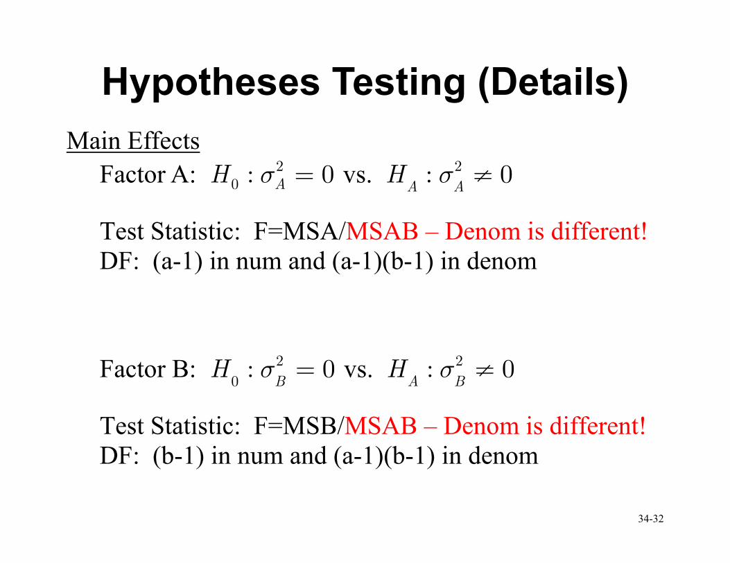
Hypotheses Testing (Details)

Main Effects

Factor A: 20 : 0AH σ = vs. 2: 0

A AH σ ≠

Test Statistic: F=MSA/MSAB – Denom is different!

DF: (a-1) in num and (a-1)(b-1) in denom

Factor B: 2

0: 0B

H σ = vs. 2: 0A BH σ ≠

Test Statistic: F=MSB/MSAB – Denom is different!

DF: (b-1) in num and (a-1)(b-1) in denom

34-33

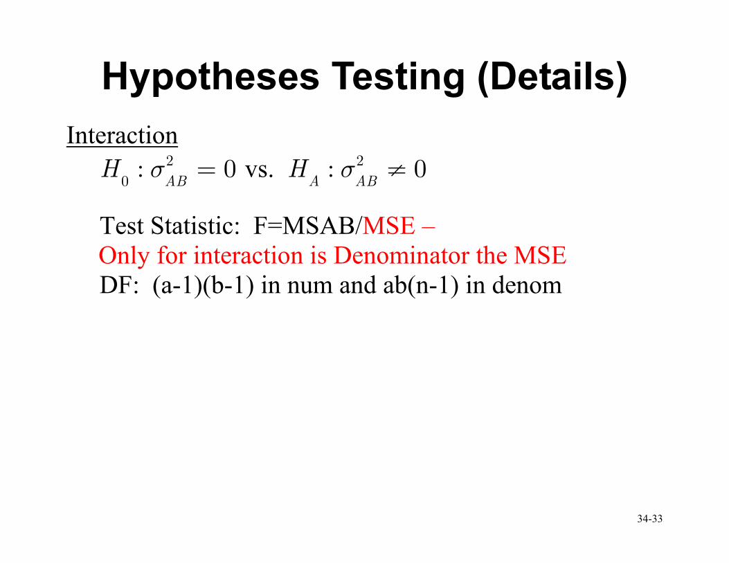
Hypotheses Testing (Details)

Interaction 2

0: 0AB

H σ = vs. 2: 0A ABH σ ≠

Test Statistic: F=MSAB/MSE –

Only for interaction is Denominator the MSE

DF: (a-1)(b-1) in num and ab(n-1) in denom

34-34

Example

• KNNL 25.15 (pg 1080)

• SAS code: mpg.sas

• Y is fuel efficiency in miles per gallon

• Factor A represents four different drivers,

a=4 levels

• Factor B represents five different cars of the

same model , b=5

• Each driver drove each car twice over the

same 40-mile test course (n = 2)

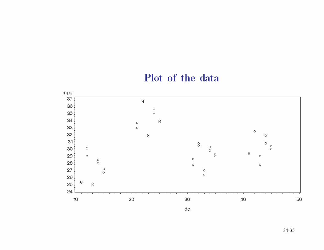
34-35

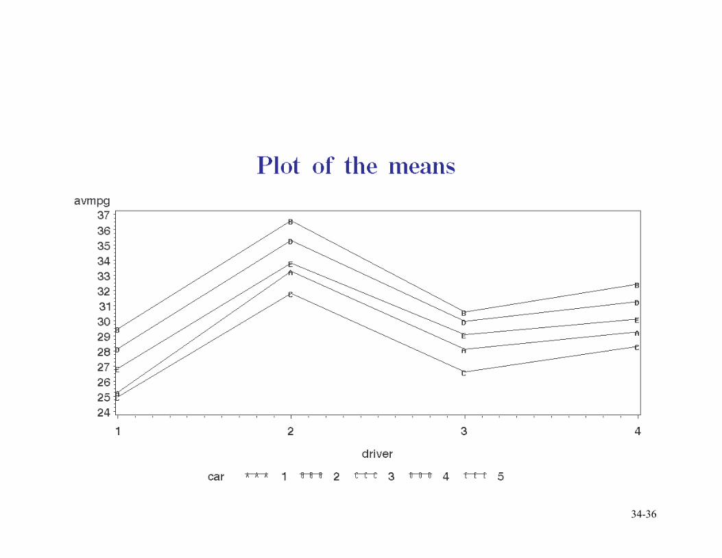
34-36

34-37

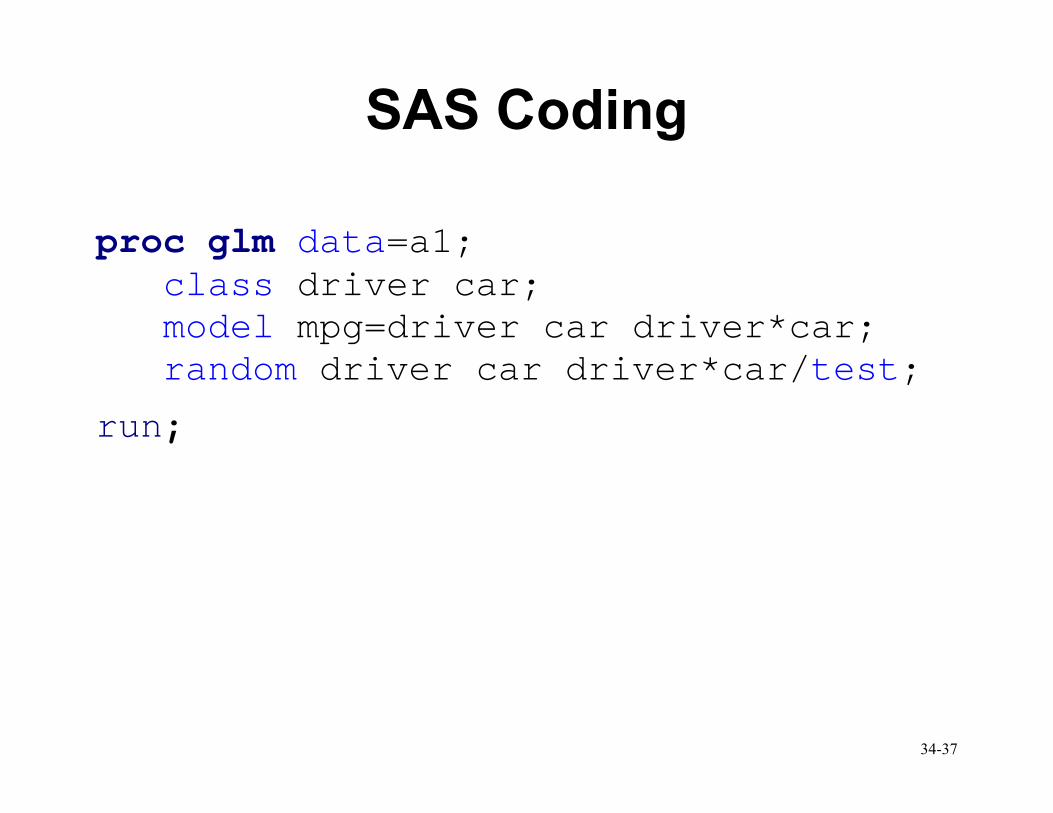
SAS Coding

proc glm data=a1; class driver car; model mpg=driver car driver*car; random driver car driver*car/test;

run;

34-38

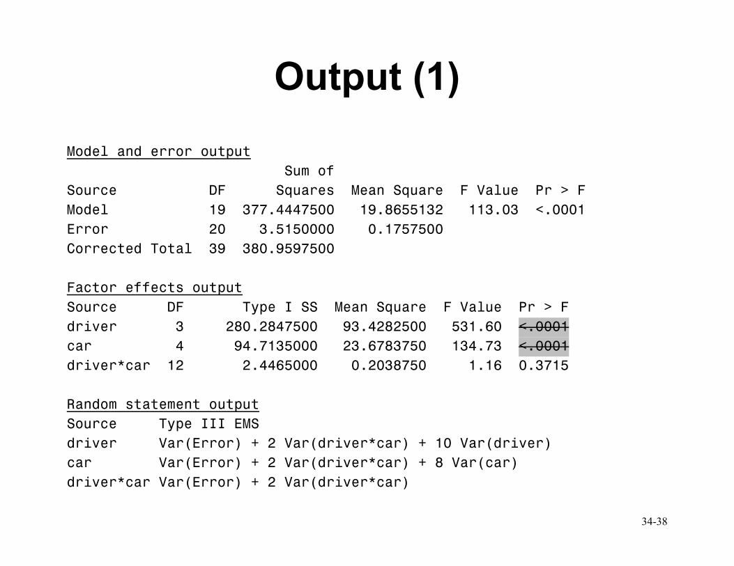
Output (1)

Model and error output

Sum of

Source DF Squares Mean Square F Value Pr > F

Model 19 377.4447500 19.8655132 113.03 <.0001

Error 20 3.5150000 0.1757500

Corrected Total 39 380.9597500

Factor effects output

Source DF Type I SS Mean Square F Value Pr > F

driver 3 280.2847500 93.4282500 531.60 <.0001

car 4 94.7135000 23.6783750 134.73 <.0001

driver*car 12 2.4465000 0.2038750 1.16 0.3715

Random statement output

Source Type III EMS

driver Var(Error) + 2 Var(driver*car) + 10 Var(driver)

car Var(Error) + 2 Var(driver*car) + 8 Var(car)

driver*car Var(Error) + 2 Var(driver*car)

34-39

Output (2)

Note that only the interaction test is valid here:

the test for interaction is MSAB/MSE, but the

tests for main effects should be MSA/MSAB and

MSB/MSAB which are done with the test

statement, not / MSE as is done here.

Lesson: just because SAS spits out a P-value,

doesn’t mean it is for a meaningful test!

34-40

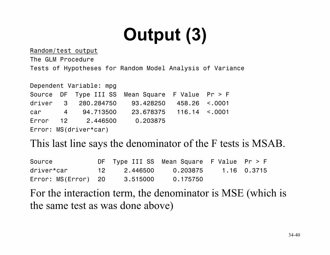
Output (3) Random/test output

The GLM Procedure

Tests of Hypotheses for Random Model Analysis of Variance

Dependent Variable: mpg

Source DF Type III SS Mean Square F Value Pr > F

driver 3 280.284750 93.428250 458.26 <.0001

car 4 94.713500 23.678375 116.14 <.0001

Error 12 2.446500 0.203875

Error: MS(driver*car)

This last line says the denominator of the F tests is MSAB.

Source DF Type III SS Mean Square F Value Pr > F

driver*car 12 2.446500 0.203875 1.16 0.3715

Error: MS(Error) 20 3.515000 0.175750

For the interaction term, the denominator is MSE (which is

the same test as was done above)

34-41

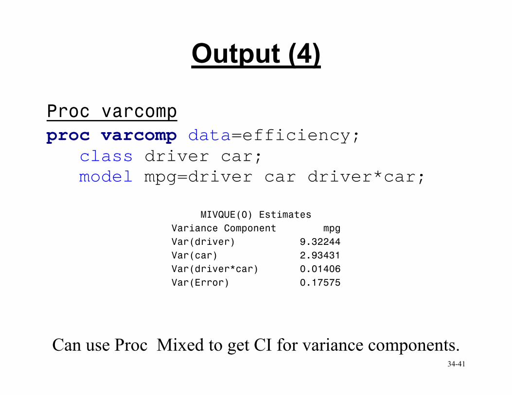
Output (4) Proc varcomp

proc varcomp data=efficiency; class driver car; model mpg=driver car driver*car;

MIVQUE(0) Estimates

Variance Component mpg

Var(driver) 9.32244

Var(car) 2.93431

Var(driver*car) 0.01406

Var(Error) 0.17575

Can use Proc Mixed to get CI for variance components.

34-42

Upcoming…

• Two-Way Mixed Model

o One Fixed Effect

o One Random Effect