meta-analysis fixed effect vs. random effects fixed effect... · meta-analysis . fixed effect vs....
TRANSCRIPT

Meta-Analysis Fixed effect vs. random effects
Michael Borenstein
Larry Hedges
Hannah Rothstein
www.Meta-Analysis.com © 2007 Borenstein, Hedges, Rothstein | 1

Section: Fixed effect vs. random effects models..................................................4
Overview ...........................................................................................................4 Fixed effect model .............................................................................................6
Definition of a combined effect.......................................................................6 Assigning weights to the studies....................................................................6
Random effects model ....................................................................................11 Definition of a combined effect.....................................................................11 Assigning weights to the studies..................................................................12
Fixed effect vs. random effects models ...........................................................22 The concept .................................................................................................22 Definition of a combined effect.....................................................................22 Computing the combined effect ...................................................................23 Extreme effect size in large study ................................................................23 Extreme effect size in small study................................................................25 Confidence interval width.............................................................................26 Which model should we use? ......................................................................29 Mistakes to avoid in selecting a model ........................................................30
Example 1 ─ Binary (2x2) Data...........................................................................32 Start the program and enter the data ..............................................................33
Insert column for study names.....................................................................34 Insert columns for the effect size data .........................................................35 Enter the data ..............................................................................................41 Show details for the computations ...............................................................42 Customize the screen ..................................................................................47 Display weights............................................................................................48
Compare the fixed effect and random effects models .....................................49 Impact of model on study weights................................................................50 Impact of model on the combined effect ......................................................51 Impact of model on the confidence interval .................................................52 What would happen if we eliminated Manning?...........................................53
Additional statistics..........................................................................................55 Test of the null hypothesis ...........................................................................56 Test of the heterogeneity .............................................................................58 Quantifying the heterogeneity ......................................................................60
High-resolution plots........................................................................................62 Computational details......................................................................................67
Computational details for the fixed effect analysis .......................................69 Computational details for the random effects analysis.................................73
Example 2 ─ Means............................................................................................77 Start the program and enter the data ..............................................................78
Insert column for study names.....................................................................79 Insert columns for the effect size data .........................................................80 Enter the data ..............................................................................................86 Show details for the computations ...............................................................87
www.Meta-Analysis.com © 2007 Borenstein, Hedges, Rothstein | 2
Run the analysis..............................................................................................89 Customize the screen ..................................................................................91 Display weights............................................................................................92
Compare the fixed effect and random effects models .....................................93 Impact of model on study weights................................................................94 Impact of model on the combined effect ......................................................95 Impact of model on the confidence interval .................................................96 What would happen if we eliminated Manning?...........................................97
Additional statistics..........................................................................................99 Test of the null hypothesis .........................................................................100 Test of the heterogeneity ...........................................................................101 Quantifying the heterogeneity ....................................................................102
High-resolution plots......................................................................................104 Computational details....................................................................................109
Computational details for the fixed effect analysis .....................................109 Computational details for the random effects analysis...............................113
Example 3 ─ Correlational Data........................................................................117 Start the program and enter the data ............................................................118
Insert column for study names...................................................................119 Insert columns for the effect size data .......................................................120 Enter the data ............................................................................................125 What are Fisher’s Z values ........................................................................126 Customize the screen ................................................................................133 Display weights..........................................................................................134
Compare the fixed effect and random effects models ...................................135 Impact of model on study weights..............................................................136 Impact of model on the combined effect ....................................................137 Impact of model on the confidence interval ...............................................138 What would happen if we eliminated Manning?.........................................139
Additional statistics........................................................................................141 Test of the null hypothesis .........................................................................142 Test of the heterogeneity ...........................................................................144 Quantifying the heterogeneity ....................................................................146
High-resolution plots......................................................................................148 Computational details....................................................................................153
Computational details for the fixed effect analysis .....................................155 Computational details for the random effects analysis...............................159
www.Meta-Analysis.com © 2007 Borenstein, Hedges, Rothstein | 3

Section: Fixed effect vs. random effects models Overview One goal of a meta-analysis will often be to estimate the overall, or combined effect. If all studies in the analysis were equally precise we could simply compute the mean of the effect sizes. However, if some studies were more precise than others we would want to assign more weight to the studies that carried more information. This is what we do in a meta-analysis. Rather than compute a simple mean of the effect sizes we compute a weighted mean, with more weight given to some studies and less weight given to others. The question that we need to address, then, is how the weights are assigned. It turns out that this depends on what we mean by a “combined effect”. There are two models used in meta-analysis, the fixed effect model and the random effects model. The two make different assumptions about the nature of the studies, and these assumptions lead to different definitions for the combined effect, and different mechanisms for assigning weights. Definition of the combined effect Under the fixed effect model we assume that there is one true effect size which is shared by all the included studies. It follows that the combined effect is our estimate of this common effect size. By contrast, under the random effects model we allow that the true effect could vary from study to study. For example, the effect size might be a little higher if the subjects are older, or more educated, or healthier; or if the study used a slightly more intensive or longer variant of the intervention; or if the effect was measured more reliably; and so on. The studies included in the meta-analysis are assumed to be a random sample of the relevant distribution of effects, and the combined effect estimates the mean effect in this distribution.
www.Meta-Analysis.com © 2007 Borenstein, Hedges, Rothstein | 4

Computing a combined effect Under the fixed effect model all studies are estimating the same effect size, and so we can assign weights to all studies based entirely on the amount of information captured by that study. A large study would be given the lion’s share of the weight, and a small study could be largely ignored. By contrast, under the random effects model we are trying to estimate the mean of a distribution of true effects. Large studies may yield more precise estimates than small studies, but each study is estimating a different effect size, and each of these effect sizes serve as a sample from the population whose mean we want to estimate. Therefore, as compared with the fixed effect model, the weights assigned under random effects are more balanced. Large studies are less likely to dominate the analysis and small studies are less likely to be trivialized. Precision of the combined effect Under the fixed effect model the only source of error in our estimate of the combined effect is the random error within studies. Therefore, with a large enough sample size the error will tend toward zero. This holds true whether the large sample size is confined to one study or distributed across many studies. By contrast, under the random effects model there are two levels of sampling and two levels of error. First, each study is used to estimate the true effect in a specific population. Second, all of the true effects are used to estimate the mean of the true effects. Therefore, our ability to estimate the combined effect precisely will depend on both the number of subjects within studies (which addresses the first source of error) and also the total number of studies (which addresses the second). In other words, even if each study had infinite sample size there would still be uncertainty in our estimate of the mean, since these studies have been sampled from all possible studies. How this section is organized The two chapters that follow provide detail on the fixed effect model and the random effects model. These chapters include computational details and worked examples for each model. Then, a chapter highlights the differences between the two.
www.Meta-Analysis.com © 2007 Borenstein, Hedges, Rothstein | 5

Fixed effect model
Definition of a combined effect In a fixed effect analysis we assume that all the included studies share a common effect size, μ. The observed effects will be distributed about μ, with a variance σ2 that depends primarily on the sample size for each study.
Fixed effect model. The observed effects are sampled from a distribution with true effect μ, and variance σ2. The observed effect T1 is equal to μ+ε i.
In this schematic the observed effect in Study 1, T1, is a determined by the common effect μ plus the within-study error ε1. More generally, for any observed effect Ti, iT μ εi= + (0.1)
Assigning weights to the studies In the fixed effect model there is only one level of sampling, since all studies are sampled from a population with effect size μ. Therefore, we need to deal with only one source of sampling error – within studies (e).
www.Meta-Analysis.com © 2007 Borenstein, Hedges, Rothstein | 6

Since our goal is to assign more weight to the studies that carry more information, we might propose to weight each study by its sample size, so that a study with 1000 subjects would get 10 times the weight of a study with 100 subjects. This is basically the approach used, except that we assign weights based on the inverse of the variance rather than sample size. The inverse variance is roughly proportional to sample size, but is a more nuanced measure (see notes), and serves to minimize the variance of the combined effect. Concretely, the weight assigned to each study is
1i
i
wv
= (0.2)
where vi is the within-study variance for study (i). The weighted mean (T • ) is then computed as
1
1
k
i ii
k
ii
w TT
w
=•
=
=∑
∑ (0.3)
that is, the sum of the products wiTi (effect size multiplied by weight) divided by the sum of the weights. The variance of the combined effect is defined as the reciprocal of the sum of the weights, or
1
1k
ii
vw
•
=
=
∑ (0.4)
and the standard error of the combined effect is then the square root of the variance, ( )SE T v• •= (0.5) The 95% confidence interval for the combined effect would be computed as 1.96 * ( )Lower Limit T SE T• •= − (0.6) 1.96 * ( )Upper Limit T SE T• •= + (0.7) Finally, if one were so inclined, the Z-value could be computed using
www.Meta-Analysis.com © 2007 Borenstein, Hedges, Rothstein | 7

( )
TZSE T
•
•
= (0.8)
For a one-tailed test the p-value would be given by 1 Φ( )p Z= − (0.9) and for a two-tailed test by ( )( )2 1 Φ | |p Z⎡ ⎤= −⎣ ⎦ ,
(0.10)
where Φ(Z) is the standard normal cumulative distribution function. Illustrative example The following figure is the forest plot of a fictional meta-analysis that looked at the impact of an intervention on reading scores in children.
In this example the Carroll study has a variance of 0.03. The weight for that study would computed as
11 33.333
(0.03)w = =
www.Meta-Analysis.com © 2007 Borenstein, Hedges, Rothstein | 8
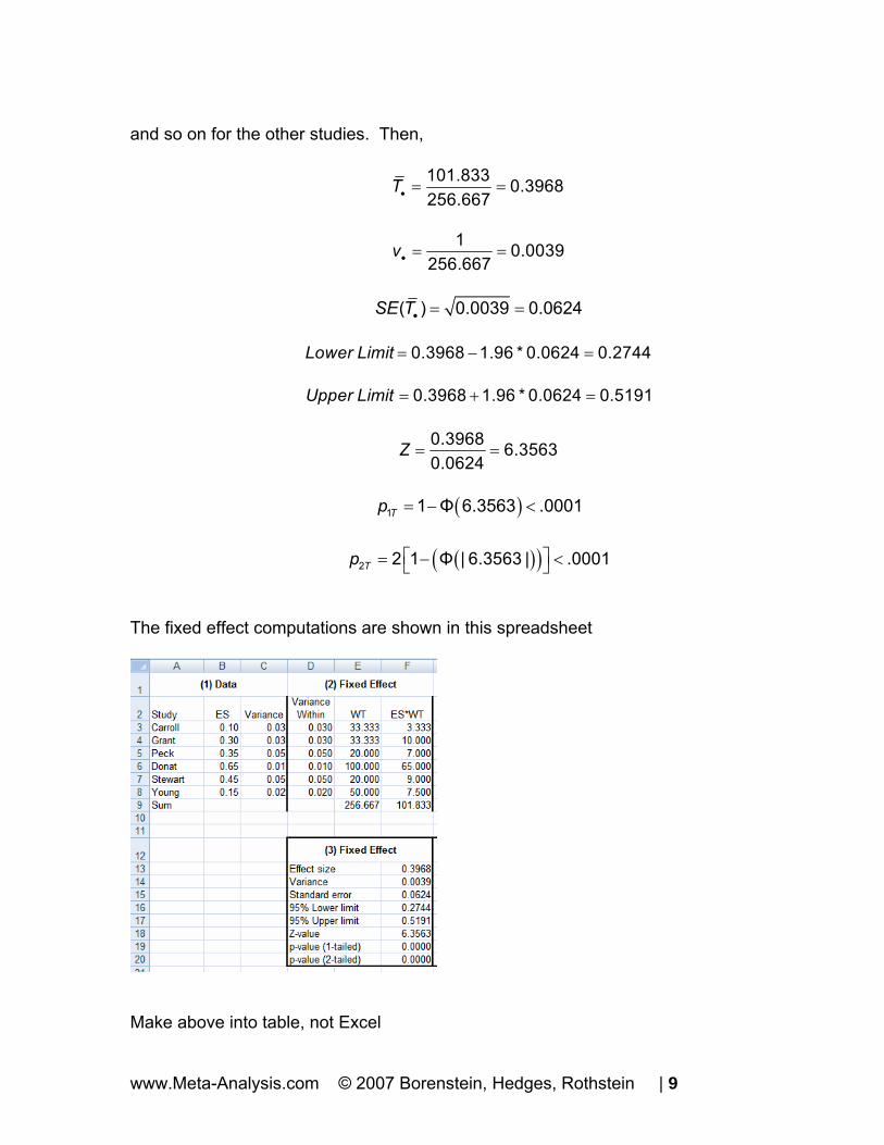
and so on for the other studies. Then,
101.833 0.3968256.667
T• = =
1 0.0039256.667
v• = =
( ) 0.0039 0.0624SE T• = = 0.3968 1.96 * 0.0624 0.2744Lower Limit = − = 0.3968 1.96 * 0.0624 0.5191Upper Limit = + =
0.3968 6.35630.0624
Z = =
( )1 1 Φ 6.3563 .0001Tp = − <
( )( )2 2 1 Φ | 6.3563 | .0001Tp ⎡ ⎤= − <⎣ ⎦
The fixed effect computations are shown in this spreadsheet
Make above into table, not Excel
www.Meta-Analysis.com © 2007 Borenstein, Hedges, Rothstein | 9

Incorporate formula refs directly into the table above Column (Cell) Label Content Excel Formula* See formula
(Section 1) Effect size and weights for each study
A Study name Entered B Effect size Entered C Variance Entered
(Section 2) Compute WT and WT*ES for each study
D Variance within study =$C3 E Weight =1/D3 (0.2) F ES*WT =$B3*E3
Sum the columns
E9 Sum of WT =SUM(E3:E8) F9 Sum of WT*ES =SUM(F3:F8)
(Section 3) Compute combined effect and related statistics
F13 Effect size =F9/E9 (0.3) F14 Variance =1/E9 (0.4) F15 Standard error =SQRT(F14) (0.5) F16 95% lower limit =F13-1.96*F15 (0.6) F17 95% upper limit =F13+1.96*F15 (0.7) F18 Z-value =F13/F15 (0.8) F19 p-value (1-tailed) =(1-(NORMDIST((F18),0,1,TRUE))) (0.9) F20 p-value (2-tailed) =(1-(NORMDIST(ABS(F18),0,1,TRUE)))*2 (0.10) Comments Some formulas include a “$”. In Excel this means that the reference is to a specific column. These are not needed here, but will be needed when we expand this spreadsheet in the next chapter to allow for other computational models. Inverse variance vs. sample size. As noted, weights are based on the inverse variance rather than the sample size. The inverse variance is determined primarily by the sample size, but it is a more nuanced measure. For example, the variance of a mean difference takes account not only of the total N, but also the sample size in each group. Similarly, the variance of an odds ratio is based not only on the total N but also on the number of subjects in each cell. The combined mean computed with inverse variance weights will have the smallest possible variance.
www.Meta-Analysis.com © 2007 Borenstein, Hedges, Rothstein | 10
Random effects model The fixed effect model, discussed above, starts with the assumption that the true effect is the same in all studies. However, this assumption may be implausible in many systematic reviews. When we decide to incorporate a group of studies in a meta-analysis we assume that the studies have enough in common that it makes sense to synthesize the information. However, there is generally no reason to assume that they are “identical” in the sense that the true effect size is exactly the same in all the studies. For example, assume that we are working with studies that compare the proportion of patients developing a disease in two groups (vaccination vs. placebo). If the treatment works we would expect the effect size (say, the risk ratio) to be similar but not identical across studies. The impact of the treatment might be more pronounced in studies where the patients were older, or where they had less natural immunity. Or, assume that we are working with studies that assess the impact of an educational intervention. The magnitude of the impact might vary depending on the other resources available to the children, the class size, the age, and other factors, which are likely to vary from study to study. We might not have assessed these covariates in each study. Indeed, we might not even know what covariates actually are related to the size of the effect. Nevertheless, experience says that such factors exist and may lead to variations in the magnitude of the effect.
Definition of a combined effect
www.Meta-Analysis.com © 2007 Borenstein, Hedges, Rothstein | 11

Rather than assume that there is one true effect, we allow that there is a distribution of true effect sizes. The combined effect therefore cannot represent the one common effect, but instead represents the mean of the population of true effects.
Random effects model. The observed effect T1 (box) is sampled from a distribution with true effect θ1, and variance σ2. This true effect θ1, in turn, is sampled from a distribution with mean μ and variance τ2.
In this schematic the observed effect in Study 1, T1, is a determined by the true effect θ1 plus the within-study error ε1. In turn, θ1, is determined by the mean of all true effects, μ and the between-study error ζ1. More generally, for any observed effect Ti, i i i iT θ ε μ ζ εi= + = + + (1.1)
Assigning weights to the studies
www.Meta-Analysis.com © 2007 Borenstein, Hedges, Rothstein | 12

Under the random effects model we need to take account of two levels of sampling, and two source of error. First, the true effect sizes θ are distributed about μ with a variance τ2 that reflects the actual distribution of the true effects about their mean. Second, the observed effect T for any given θ will be distributed about that θ with a variance σ2 that depends primarily on the sample size for that study. Therefore, in assigning weights to estimate μ, we need to deal with both sources of sampling error – within studies (ε), and between studies (ζ). Decomposing the variance The approach of a random effects analysis is to decompose the observed variance into its two component parts, within-studies and between-studies, and then use both parts when assigning the weights. The goal will be to take account of both sources of imprecision. The mechanism used to decompose the variance is to compute the total variance (which is observed) and then to isolate the within-studies variance. The difference between these two values will give us the variance between-studies, which is called tau-squared (τ2). Consider the three graphs in the following figure.
www.Meta-Analysis.com © 2007 Borenstein, Hedges, Rothstein | 13

In (A) the studies all line up pretty much in a row. There is no variance between studies, and therefore tau-squared is low (or zero). In (B) there is variance between studies, but it is fully explained by the variance within studies. Put another way, given the imprecision of the studies, we would expect the effect size to vary somewhat from one study to the next. Therefore, the between-studies variance is again low (or zero). In (C) there is variance between studies. And, it cannot be fully explained by the variance within studies, since the within-study variance is minimal. The excess variation (between-studies variance), will be reflected in the value of tau-squared. It follows that tau-squared will increase as either the variance within-studies decreases and/or the observed variance increases. This logic is operationalized in a series of formulas. We will compute Q, which represents the total variance, and df, which represents the expected variance if all studies have the same true effect. The difference, Q - df, will give us the excess variance. Finally, this value will be transformed, to put it into the same scale as the within-study variance. This last value is called tau-squared (τ2). The Q statistic represents the total variance and is defined as
( )2
1
k
i ii
Q w T T •
== −∑ (1.2)
that is, the sum of the squared deviations of each study (Ti) from the combined mean ( .T ). Note the “wi” in the formula, which indicates that each of the squared deviations is weighted by the study’s inverse variance. A large study that falls far from the mean will have more impact on Q than would a small study in the same location. An equivalent formula, useful for computations, is
2
12
1
1
k
i iki
i i ki
ii
w TQ w T
w
=
=
=
⎛ ⎞⎜ ⎟⎝= −∑
∑∑
⎠ (1.3)
Since Q reflects the total variance, it must now be broken down into its component parts. If the only source of variance was within-study error, then the expected value of Q would be the degrees of freedom (df) for the meta-analysis where
www.Meta-Analysis.com © 2007 Borenstein, Hedges, Rothstein | 14

(df Number Studies) 1= − (1.4) This allows us to compute the between-studies variance, τ2, as
if Q > df
0 if Q df
Q dfτ C2
−⎧⎪= ⎨⎪ ≤⎩
(1.5)
where
2i
ii
wC w
w= − ∑∑ ∑
(1.6)
The numerator, Q - df, is the excess (observed minus expected) variance. The denominator, C, is a scaling factor that has to do with the fact that Q is a weighted sum of squares. By applying this scaling factor we ensure that tau-squared is in the same metric as the variance within-studies. In the running example,
2101.83353.208 12.8056
256.667Q
⎛ ⎞= − =⎜ ⎟
⎝ ⎠
(6 1) 5df = − =
15522.222256.667 196.1905256.667
C ⎛ ⎞= − =⎜ ⎟⎝ ⎠
2 12.8056 5 0.0398196.1905
τ −= =
Assigning weights under the random effects model In the fixed effect analysis each study was weighted by the inverse of its variance. In the random effects analysis, too, each study will be weighted by the inverse of its variance. The difference is that the variance now includes the original (within-studies) variance plus the between-studies variance, tau-squared. Note the correspondence between the formulas here and those in the previous chapter. We use the same notations, but add a (*) to represent the random effects version. Concretely, under the random effects model the weight assigned to each study is
www.Meta-Analysis.com © 2007 Borenstein, Hedges, Rothstein | 15

**
1i
i
wv
= (1.7)
where v*i is the within-study variance for study (i) plus the between-studies variance, tau-squared. That is, * 2
i iv v τ= + . The weighted mean (T• *) is then computed as
*
1
*
1
*
k
i ii
k
ii
w TT
w
=•
=
=∑
∑ (1.8)
that is, the sum of the products (effect size multiplied by weight) divided by the sum of the weights. The variance of the combined effect is defined as the reciprocal of the sum of the weights, or
*.
*
1
1k
ii
vw
=
=
∑ (1.9)
and the standard error of the combined effect is then the square root of the variance, ( *) *SE T v• = • (1.10) The 95% confidence interval for the combined effect would be computed as * * 1.96 * ( *)Lower Limit T SE T•= − • (1.11) * * 1.96 * ( *)Upper Limit T SE T•= + • (1.12) Finally, if one were so inclined, the Z-value could be computed using
* *( *)
TZSE T
•
•
= (1.13)
www.Meta-Analysis.com © 2007 Borenstein, Hedges, Rothstein | 16

The one-tailed p-value (assuming an effect in the hypothesized direction) is given by ( )* 1 Φ *p Z= − (1.14)
and the two-tailed p-value by ( )* 2 1 Φ | |p *Z⎡ ⎤= −⎣ ⎦ (1.15)
where Φ(Z) is the standard normal cumulative distribution function. Illustrative example The following figure is based on the same studies we used for the fixed effect example.
Note the differences from the fixed effect model.
• The weights are more balanced. The boxes for the large studies such as Donat have decreased in area while those for the small studies such as Peck have increase in area.
• The combined effect has moved toward the left, from 0.40 to 0.34. This reflects the fact that the impact of Donat (on the right) has been reduced.
• The confidence interval for the combined effect has increased in width.
www.Meta-Analysis.com © 2007 Borenstein, Hedges, Rothstein | 17
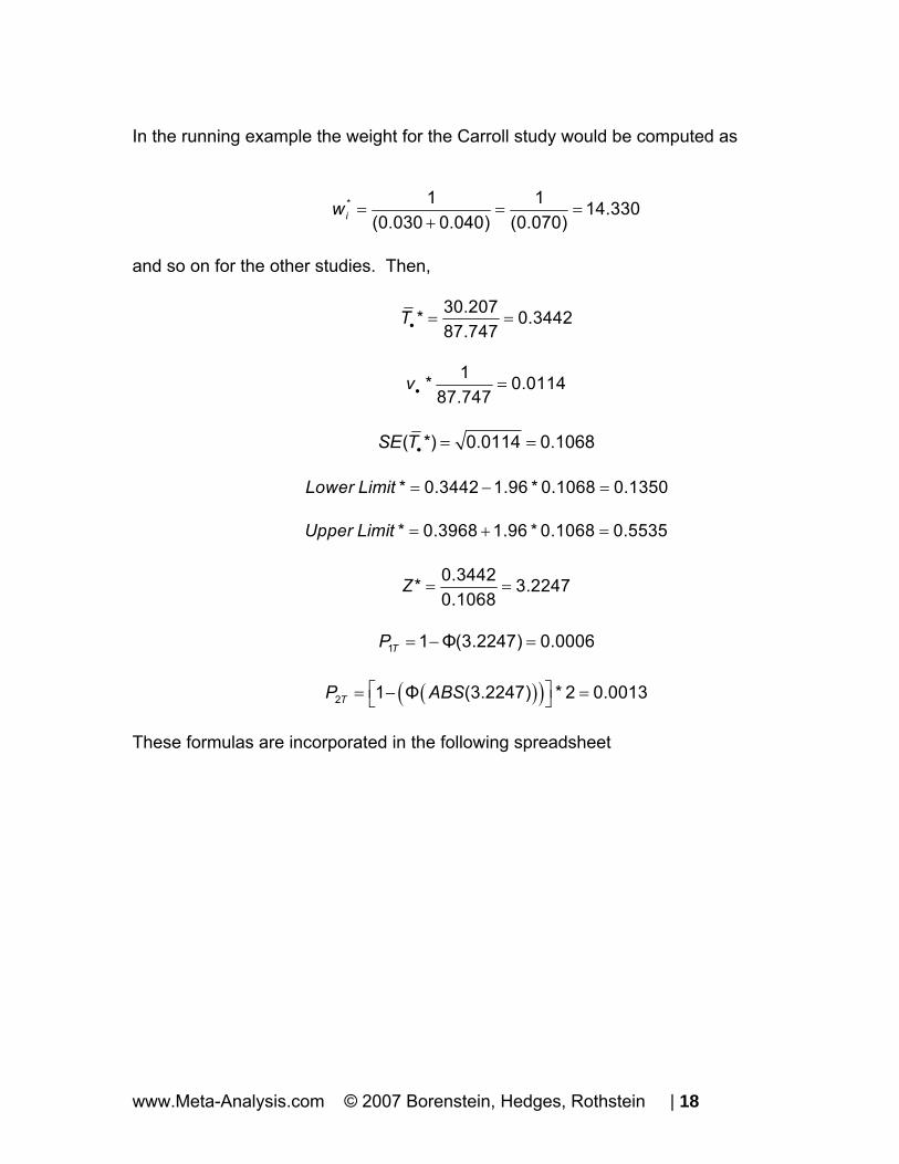
In the running example the weight for the Carroll study would be computed as
* 1 1 14.330(0.030 0.040) (0.070)iw = = =
+
and so on for the other studies. Then,
30.207* 0.87.747
T• = = 3442
1* 0.011487.747
v• =
( *) 0.0114 0.1068SE T• = = * 0.3442 1.96 * 0.1068 0.1350Lower Limit = − = * 0.3968 1.96 * 0.1068 0.5535Upper Limit = + =
0.3442* 3.22470.1068
Z = =
1 1 Φ(3.2247) 0.0006TP = − = ( )( )2 1 Φ (3.2247) * 2 0.0013TP ABS⎡ ⎤= − =⎣ ⎦
These formulas are incorporated in the following spreadsheet
www.Meta-Analysis.com © 2007 Borenstein, Hedges, Rothstein | 18

This spreadsheet builds on the spreadsheet for a fixed effect analysis. Columns A-F are identical to those in that spreadsheet. Here, we add columns for tau-squared (columns G-H) and random effects analysis (columns I-M). Note that the formulas for fixed effect and random effects analyses are identical, the only difference being the definition of the variance. For the fixed effect analysis the variance (Column D) is defined as the variance within-studies (for example D3=$C3). For the random effects analysis the variance is defined as the variance within-studies plus the variance between-studies (for example, K3=I3+J3).
www.Meta-Analysis.com © 2007 Borenstein, Hedges, Rothstein | 19

Column (Cell) Label Content Excel Formula* See formula
(Section 1) Effect size and weights for each study
A Study name Entered B Effect size Entered C Variance Entered
(Section 2) Compute fixed effect WT and WT*ES for each study
D Variance within study =$C3 E Weight =1/D3 (0.2) F ES*WT =$B3*E3
Sum the columns
E9 Sum of WT =SUM(E3:E8) F9 Sum of WT*ES =SUM(F3:F8)
(Section 3) Compute combined effect and related statistics for fixed effect model
F13 Effect size =F9/E9 (0.3) F14 Variance =1/E9 (0.4) F15 Standard error =SQRT(F14) (0.5) F16 95% lower limit =F13-1.96*F15 (0.6) F17 95% upper limit =F13+1.96*F15 (0.7) F18 Z-value =F13/F15 (0.8) F19 p-value (1-tailed) =(1-(NORMDIST((F18),0,1,TRUE))) (0.9) F20 p-value (2-tailed) =(1-(NORMDIST(ABS(F18),0,1,TRUE)))*2 (0.10)
(Section 4) Compute values needed for tau-squared
G3 ES^2*WT =B3^2*E3 H3 WT^2 =E3^2 Sum the columns G9 Sum of ES^2*WT =SUM(G3:G8) H9 Sum of WT^2 =SUM(H3:H8)
(Section 5) Compute tau-squared
H13 Q =G9-F9^2/E9 (1.3) H14 Df =COUNT(B3:B8)-1 (1.4) H15 Numerator =MAX(H13-H14,0) H16 C =E9-H9/E9 (1.6) H17 tau-sq =H15/H16 (1.5)
(Section 6) Compute random effects WT and WT*ES for each study
I3 Variance within =$C3 J3 Variance between =$H$17 K3 Variance total =I3+J3 L3 WT =1/K3 (1.7) M3 ES*WT =$B3*L3
Sum the columns
L9 Sum of WT =SUM(L3:L8) M9 Sum of ES*WT =SUM(M3:M8)
(Section 7) Compute combined effect and related statistics for random effects model
M13 Effect size =M9/L9 (1.8) M14 Variance =1/L9 (1.9) M15 Standard error =SQRT(M14) (1.10) M16 95% lower limit =M13-1.96*M15 (1.11)
www.Meta-Analysis.com © 2007 Borenstein, Hedges, Rothstein | 20

M17 95% upper limit =M13+1.96*M15 (1.12) M18 Z-value =M13/M15 (1.13) M19 p-value (1-tailed) =(1-(NORMDIST((M18),0,1,TRUE))) (1.14) M20 p-value (2-tailed) =(1-(NORMDIST(ABS(M18),0,1,TRUE)))*2 (1.15)
www.Meta-Analysis.com © 2007 Borenstein, Hedges, Rothstein | 21

Fixed effect vs. random effects models In the previous two chapters we outlined the two basic approaches to meta-analysis – the Fixed effect model and the Random effects model. This chapter will discuss the differences between the two.
The concept The fixed effect and random effects models represent two conceptually different approaches. Fixed effect The fixed effect model assumes that all studies in the meta-analysis share a common true effect size. Put another way, all factors which could influence the effect size are the same in all the study populations, and therefore the effect size is the same in all the study populations. It follows that the observed effect size varies from one study to the next only because of the random error inherent in each study. Random effects By contrast, the random effects model assumes that the studies were drawn from populations that differ from each other in ways that could impact on the treatment effect. For example, the intensity of the intervention or the age of the subjects may have varied from one study to the next. It follows that the effect size will vary from one study to the next for two reasons. The first is random error within studies, as in the fixed effect model. The second is true variation in effect size from one study to the next.
Definition of a combined effect The meaning of the “combined effect” is different for fixed effect vs. random effects analyses. Fixed effect Under the fixed effect model there is one true effect size. It follows that the combined effect is our estimate of this value. Random effects
www.Meta-Analysis.com © 2007 Borenstein, Hedges, Rothstein | 22

Under the random effects model there is not one true effect size, but a distribution of effect sizes. It follows that the combined estimate is not an estimate of one value, but rather is meant to be the average of a distribution of values.
Computing the combined effect These differences in the definition of the combined effect lead to differences in the way the combined effect is computed. Fixed effect Under the fixed effect model we assume that the true effect size for all studies is identical, and the only reason the effect size varies between studies is random error. Therefore, when assigning weights to the different studies we can largely ignore the information in the smaller studies since we have better information about the same effect size in the larger studies. Random effects By contrast, under the random effects model the goal is not to estimate one true effect, but to estimate the mean of a distribution of effects. Since each study provides information about an effect size in a different population, we want to be sure that all the populations captured by the various studies are represented in the combined estimate. This means that we cannot discount a small study by giving it a very small weight (the way we would in a fixed effect analysis). The estimate provided by that study may be imprecise, but it is information about a population that no other study has captured. By the same logic we cannot give too much weight to a very large study (the way we might in a fixed effect analysis). Our goal is to estimate the effects in a range of populations, and we do not want that overall estimate to be overly influenced by any one population.
Extreme effect size in large study How will the selection of a model influence the overall effect size? Consider the case where there is an extreme effect in a large study. Here, we have five small studies (Studies A-E, with 100 subjects per study) and one large study (Study F, with 1000 subjects). The confidence interval for each of the studies A-E is wide, reflecting relatively poor precision, while the confidence interval for Study F is narrow, indicating greater precision. In this example the small studies all have relatively large effects (in the range of 0.40 to 0.80) while the large study has a relatively small effect (0.20).
www.Meta-Analysis.com © 2007 Borenstein, Hedges, Rothstein | 23

Fixed effect Under the fixed effect model these studies are all estimating the same effect size, and the large study (F) provides a more precise estimate of this effect size. Therefore, this study is assigned 68% of the weight in the combined effect, with each of the remaining studies being assigned about 6% of the weight (see the column labeled “Relative weight” under fixed effects.
Because Study F is assigned so much of the weight it “pulls” the combined estimate toward itself. Study F had a smaller effect than the other studies and so it pulls the combined estimate toward the left. On the graph, note the point estimate for the large study (Study F, with d=.2), and how it has “pulled” the fixed effect estimate down to 0.34 (see the shaded row marked “Fixed” at the bottom of the plot). Random effects By contrast, under the random effects model these studies are drawn from a range of populations in which the effect size varies and our goal is to summarize this range of effects. Each study is estimating an effect size for its unique population, and so each must be given appropriate weight in the analysis. Now, Study F is assigned only 23% of the weight (rather than 68%), and each of the small studies is given about 15% of the weight (rather than 6%) (see the column labeled “Relative weights” under random effects). What happens to our estimate of the combined effect when we weight the studies this way? The overall effect is still being pulled by the large study, but not as much as before. In the plot, the bottom two lines reflect the fixed effect and random effect estimates, respectively. Compare the point estimate for “Random” (the last line) with the one for “Fixed” just above it. The overall effect is now 0.55 (which is much closer to the range of the small studies) rather than 0.34 (as it was for the fixed effect model). The impact of the large study is now less pronounced.
www.Meta-Analysis.com © 2007 Borenstein, Hedges, Rothstein | 24

Extreme effect size in small study Now, let’s consider the reverse situation: The effect sizes for each study are the same as in the prior example, but this time the first 5 studies are large while the sixth study is small. Concretely, we have five large studies (A-E, with 1000 subjects per study) and one small study (F, with 100 subjects). On the graphic, the confidence intervals for studies A-E are each relatively narrow, indicating high precision, while that for Study F is relatively wide, indicating less precision. The large studies all have relatively large effects (in the range of 0.40 to 0.80) while the small study has a relatively small effect (0.20). Fixed effect Under the fixed effect model the large studies (A-E) are each assigned about 20% of the weight, while the small study (F) is assigned only about 2% of the weight (see column labeled “Relative weights” under Fixed effect). This follows from the logic of the fixed effect model. The larger studies provide a good estimate of the common effect, and the small study offers a less reliable estimate of that same effect, so it is assigned a small (in this case trivial) weight. With only 2% of the weight, Study F has little impact on the combined value, which is computed as 0.64.
Random effects By contrast, under the random effects model each study is estimating an effect size for its unique population, and so each must be assigned appropriate weight in the analysis. As shown in the column “Relative weights” under random effects each of the large studies (A-E) is now assigned about 18% of the weight (rather than 20%) while the small study (F) receives 8% of the weight (rather than 2%).
www.Meta-Analysis.com © 2007 Borenstein, Hedges, Rothstein | 25
What happens to our estimate of the combined effect when we weight the studies this way? Where the small study has almost no impact under the fixed effect model, it now has a substantially larger impact. Concretely, it gets 8% of the weight, which is nearly half the weight assigned to any of the larger studies (18%). The small study therefore has more of an impact now than it did under the fixed effect model. Where it was assigned only 2% of the weight before, it is now assigned 8% of the weight. This is 50% of the weight assigned to studies A-E, and as such is no longer a trivial amount. Compare the two lines labeled “Fixed” and “Random” at the bottom of the plot. The overall effect is now 0.61, which is .03 points closer to study F than it had been under the fixed effect model (0.64). Summary The operating premise, as illustrated in these examples, is that the relative weights assigned under random effects will be more balanced than those assigned under fixed effects. As we move from fixed effect to random effects, extreme studies will lose influence if they are large, and will gain influence if they are small. In these two examples we included a single study with an extreme size and an extreme effect, to highlight the difference between the two weighting schemes. In most analyses, of course, there will be a range of sample sizes within studies and the larger (or smaller) studies could fall anywhere in this range. Nevertheless, the same principle will hold.
Confidence interval width Above, we considered the impact of the model (fixed vs. random effects) on the combined effect size. Now, let’s consider the impact on the width of the confidence interval. Recall that the fixed effect model defines “variance” as the variance within a study, while the random effects model defines it as variance within a study plus variance between studies. To understand how this difference will affect the width of the confidence interval, let’s consider what would happen if all studies in the meta-analysis were of infinite size, which means that the within-study error is effectively zero. Fixed effect Since we’ve started with the assumption that all variation is due to random error, and this error has now been removed, it follows that
• The observed effects would all be identical.
www.Meta-Analysis.com © 2007 Borenstein, Hedges, Rothstein | 26

• The combined effect would be exactly the same as each of the individual studies.
• The width of the confidence interval for the combined effect would approach zero.
All of these points can be seen in the figure. In particular, note that the diamond representing the combined effect has a width of zero, since the width of the confidence interval is zero.
Study name Std diff in means and 95% CI
Std diff Standard in means error
A 0.400 0.001B 0.400 0.001C 0.400 0.001D 0.400 0.001E 0.400 0.001
0.400 0.000
-1.00 -0.50 0.00 0.50 1.00
Favours A Favours B
Fixed effect model with huge N
Meta Analysis
Generally, we are concerned with the precision of the combined effect rather than the precision of the individual studies. For this purpose it doesn’t matter whether the sample is concentrated in one study or dispersed among many studies. In either case, as the total N approaches infinity the errors will cancel out and the standard error will approach zero. Random effects Under the random effects model the effect size for each study would still be known precisely. However, the effects would not line up in a row since the true treatment effect is assumed to vary from one study to the next. It follows that –
• The within-study error would approach zero, and the width of the confidence interval for each study would approach zero.
www.Meta-Analysis.com © 2007 Borenstein, Hedges, Rothstein | 27

• Since the studies are all drawn from different populations, even though the effects are now being estimated without error, the observed effects would not be identical to each other.
• The width of the confidence interval for the combined effect would not
approach zero unless the number of studies approached infinity. Generally, we are concerned with the precision of the combined effect rather than the precision of the individual studies. Under the random effects model we need an infinite number of studies in order for the standard error in estimating μ to approach zero. In our example we know the value of the five effects precisely, but these are only a random sample of all possible effects, and so there remains substantial error in our estimate of the mean effect. Note. While the distribution of the θ i about μ represents a real distribution of effect sizes, we nevertheless refer to this as “error” since it introduces error into our estimate of the mean effect. If the studies that we do observe tend to cluster closely together and/or our meta-analysis includes a large number of studies, this source of error will tend to be small. If the studies that we do observe show much dispersion and/or we have only a small sample of studies, then this source of error will tend to be large.
Study name Std diff in means and 95% CI
Std diff Standard in means error
A 0.400 0.001B 0.450 0.001C 0.350 0.001D 0.450 0.001E 0.350 0.001
0.400 0.022
-1.00 -0.50 0.00 0.50 1.00
Favours A Favours B
Random effects model with huge N
Meta Analysis
www.Meta-Analysis.com © 2007 Borenstein, Hedges, Rothstein | 28

Summary Since the variation under random effects incorporates the same error as fixed effects plus an additional component, it cannot be less than the variation under the fixed effect model. As long as the between-studies variation is non-zero, the variance, standard error, and confidence interval will always be larger under random effects. The standard error of the combined effect in both models is inversely proportional to the number of studies. Therefore, in both models, the width of the confidence interval tends toward zero as the number of studies increases. In the case of the fixed effect model the standard error and the width of the confidence interval can tend toward zero even with a finite number of studies if any of the studies is sufficiently large. By contrast, for the random effects model, the confidence interval can tend toward zero only with an infinite number of studies (unless the between-study variation is zero).
Which model should we use? The selection of a computational model should be based on the nature of the studies and our goals. Fixed effect The fixed effect model makes sense if (a) there is reason to believe that all the studies are functionally identical, and (b) our goal is to compute the common effect size, which would then be generalized to other examples of this same population. For example, assume that a drug company has run five studies to assess the effect of a drug. All studies recruited patients in the same way, used the same researchers, dose, and so on, so all are expected to have the identical effect (as though this were one large study, conducted with a series of cohorts). Also, the regulatory agency wants to see if the drug works in this one population. In this example, a fixed effect model makes sense. Random effects By contrast, when the researcher is accumulating data from a series of studies that had been performed by other people, it would be unlikely that all the studies were functionally equivalent. Typically, the subjects or interventions in these studies would have differed in ways that would have impacted on the results, and therefore we should not assume a common effect size. Therefore, in these
www.Meta-Analysis.com © 2007 Borenstein, Hedges, Rothstein | 29

cases the random effects model is more easily justified than the fixed effect model. Additionally, the goal of this analysis is usually to generalize to a range of populations. Therefore, if one did make the argument that all the studies used an identical, narrowly defined population, then it would not be possible to extrapolate from this population to others, and the utility of the analysis would be limited. Note If the number of studies is very small, then it may be impossible to estimate the between-studies variance (tau-squared) with any precision. In this case, the fixed effect model may be the only viable option. In effect, we would then be treating the included studies as the only studies of interest.
Mistakes to avoid in selecting a model Some have adopted the practice of starting with the fixed effect model and then moving to a random effects model if Q is statistically significant. This practice should be discouraged for the following reasons.
• If the logic of the analysis says that the study effect sizes have been sampled from a distribution of effect sizes then the random effects formula, which reflects this idea, is the logical one to use.
• If the actual dispersion turns out to be trivial (that is, less than expected
under the hypothesis of homogeneity), then the random effects model will reduce to the fixed effect model. Therefore, there is no “cost” to using the random effects model in this case.
• If the actual dispersion turns out to be non-trivial, then this dispersion
should be incorporated in the analysis, which the random effects model does, and the fixed effect model does not. That the Q statistic meets or does not meet a criterion for significance is simply not relevant.
The last statement above would be true even if the Q test did a good job of identifying dispersion. In fact, though, if the number of studies is small and the within-studies variance is large, the test based on the Q statistic may have low power even if the between-study variance is substantial. In this case, using the Q test as a criterion for selecting the model is problematic not only from a conceptual perspective, but could also lead to the use of a fixed effect analysis in cases with substantial dispersion.
www.Meta-Analysis.com © 2007 Borenstein, Hedges, Rothstein | 30

www.Meta-Analysis.com © 2007 Borenstein, Hedges, Rothstein | 31
Example 1 ─ Binary (2x2) Data This appendix shows how to use Comprehensive Meta-Analysis (CMA) to perform a meta-analysis for odds ratios using fixed and random effects models. To download a free trial copy of CMA go to www.Meta-Analysis.com If your trial copy has expired, simply ask for a free extension
• Start the program • Click “I want to get an unlock code”, to create an e-mail • In the e-mail, ask for an extension • We’ll send a code by return e-mail
www.Meta-Analysis.com © 2007 Borenstein, Hedges, Rothstein | 32

Start the program and enter the data
Start CMA The program shows this dialog box.
Select START A BLANK SPREADSHEET Click OK
www.Meta-Analysis.com © 2007 Borenstein, Hedges, Rothstein | 33

The program displays this screen.
Insert column for study names
Click INSERT > COLUMN FOR > STUDY NAMES
The program has added a column for Study names.
www.Meta-Analysis.com © 2007 Borenstein, Hedges, Rothstein | 34
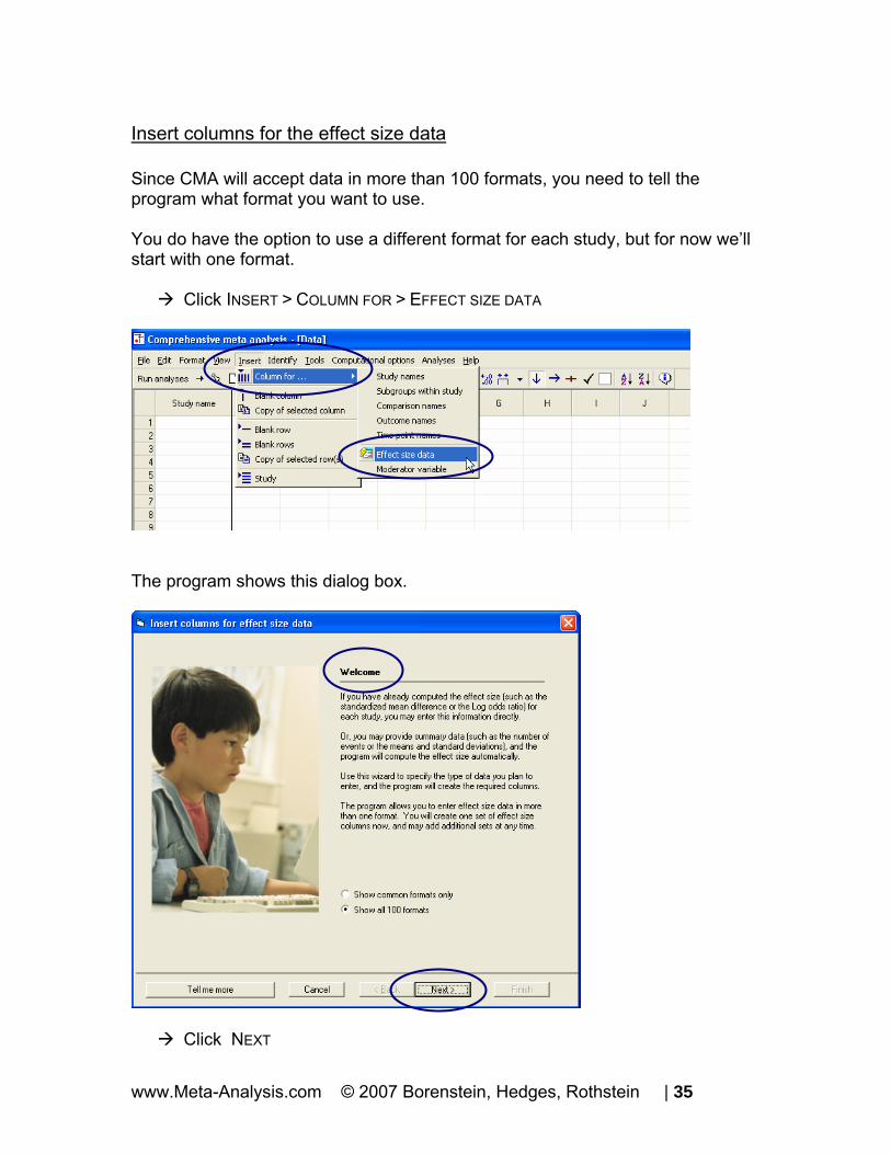
Insert columns for the effect size data Since CMA will accept data in more than 100 formats, you need to tell the program what format you want to use. You do have the option to use a different format for each study, but for now we’ll start with one format.
Click INSERT > COLUMN FOR > EFFECT SIZE DATA
The program shows this dialog box.
Click NEXT
www.Meta-Analysis.com © 2007 Borenstein, Hedges, Rothstein | 35

The dialog box lists four sets of effect sizes.
Select COMPARISON OF TWO GROUPS, TIME-POINTS, OR EXPOSURES (INCLUDES CORRELATIONS)
Click NEXT
www.Meta-Analysis.com © 2007 Borenstein, Hedges, Rothstein | 36

The program displays this dialog box.
Drill down to
DICHOTOMOUS (NUMBER OF EVENTS) UNMATCHED GROUPS, PROSPECTIVE (E.G. CONTROLLED TRIALS, COHORT
STUDIES) EVENTS AND SAMPLE SIZE IN EACH GROUP
Click FINISH
www.Meta-Analysis.com © 2007 Borenstein, Hedges, Rothstein | 37

www.Meta-Analysis.com © 2007 Borenstein, Hedges, Rothstein | 38 www.Meta-Analysis.com © 2007 Borenstein, Hedges, Rothstein | 38

The program will return to the main data-entry screen. The program displays a dialog box that you can use to name the groups.
Enter the names TREATED and CONTROL for the group Enter DIED and ALIVE for the outcome Click OK
www.Meta-Analysis.com © 2007 Borenstein, Hedges, Rothstein | 39

The program displays the columns needed for the selected format (Treated Died, Treated Total N, Control Died, Control Total N). You will enter data into the white columns (at left). The program will compute the effect size for each study and display that effect size in the yellow columns (at right). Since you elected to enter events and sample size, the program initially displays columns for the odds ratio and the log odds ratio. You can add other indices as well.
www.Meta-Analysis.com © 2007 Borenstein, Hedges, Rothstein | 40
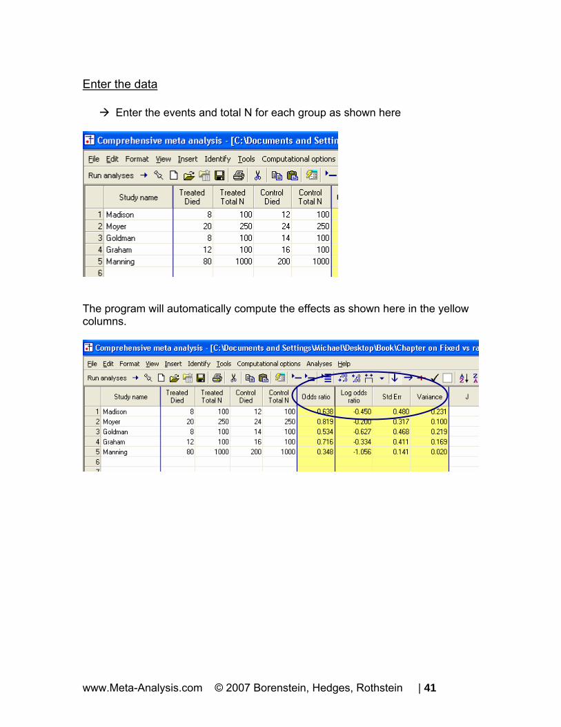
Enter the data
Enter the events and total N for each group as shown here
The program will automatically compute the effects as shown here in the yellow columns.
www.Meta-Analysis.com © 2007 Borenstein, Hedges, Rothstein | 41

Show details for the computations
Double click on the value 0.638
The program shows how this value was computed.
www.Meta-Analysis.com © 2007 Borenstein, Hedges, Rothstein | 42

Set the default index At this point, the program has displayed the odds ratio and the log odds ratio, which we’ll be using in this example. You have the option of adding additional indices, and/or specifying which index should be used as the “Default” index when you run the analysis.
Right-click on any of the yellow columns Select CUSTOMIZE COMPUTED EFFECT SIZE DISPLAY
www.Meta-Analysis.com © 2007 Borenstein, Hedges, Rothstein | 43

The program displays this dialog box.
Check Risk ratio, Log risk ratio, Risk difference Click OK
• The program has added columns for these indices
www.Meta-Analysis.com © 2007 Borenstein, Hedges, Rothstein | 44
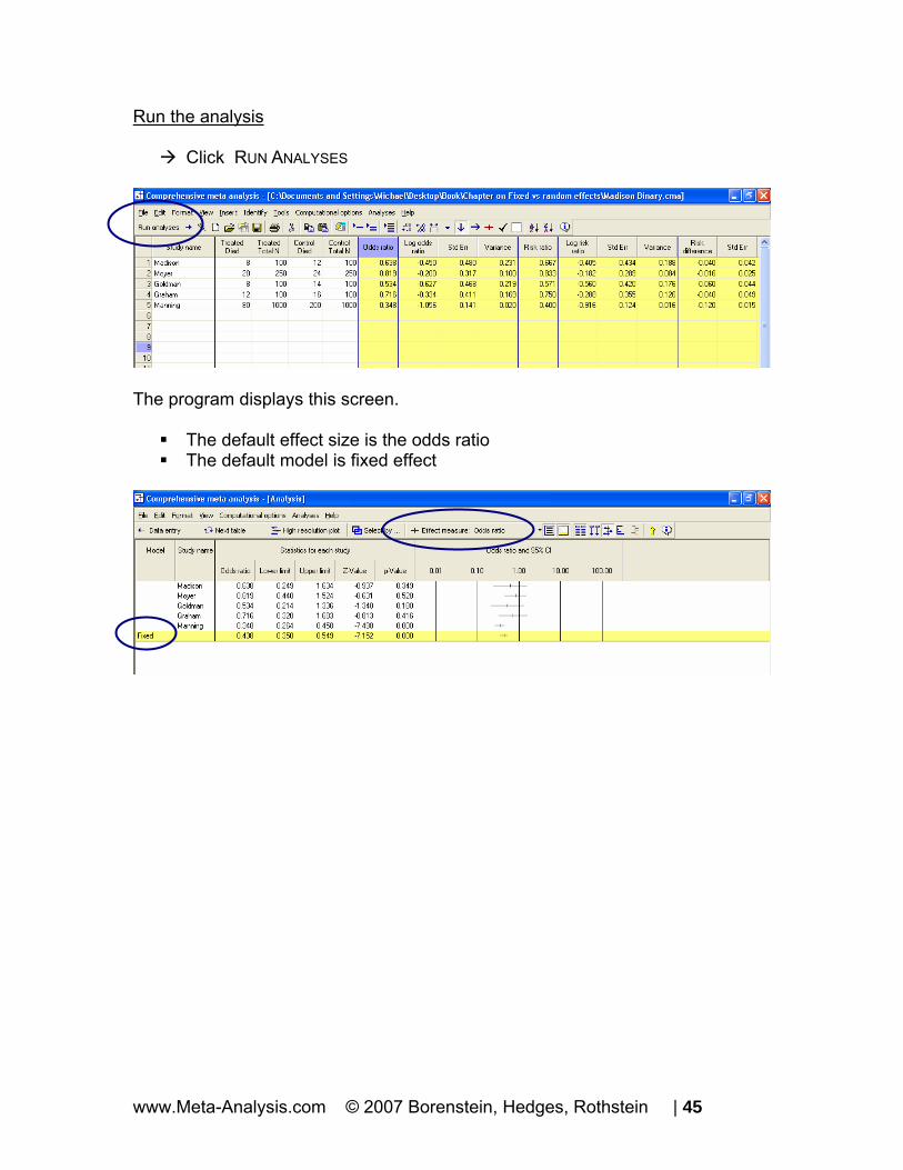
Run the analysis
Click RUN ANALYSES
The program displays this screen.
The default effect size is the odds ratio The default model is fixed effect
www.Meta-Analysis.com © 2007 Borenstein, Hedges, Rothstein | 45

The screen should look like this.
We can immediately get a sense of the studies and the combined effect. For example,
• All the effects fall below 1.0, in the range of 0.350 to 0.820. The treated group did better than the control group in all studies
• Some studies are clearly more precise than others. The confidence interval for Madison is substantially wider than the one for Manning, with the other three studies falling somewhere in between
• The combined effect is 0.438 with a 95% confidence interval of 0.350 to 0.549
www.Meta-Analysis.com © 2007 Borenstein, Hedges, Rothstein | 46

Customize the screen We want to hide the column for the z-value.
Right-click on one of the “Statistics” columns Select CUSTOMIZE BASIC STATS
Assign check-marks as shown here Click OK
Note – the standard error and variance are never displayed for the odds ratio. They are displayed when the corresponding boxes are checked and Log odds ratio is selected as the index.
www.Meta-Analysis.com © 2007 Borenstein, Hedges, Rothstein | 47

The program has hidden some of the columns, leaving us more room to work with on the display.
Display weights
Click the tool for SHOW WEIGHTS
The program now shows the relative weight assigned to each study for the fixed effect analysis. By “relative weight” we mean the weights as a percentage of the total weights, with all relative weights summing to 100%. For example, Madison was assigned a relative weight of 5.77% while Manning was assigned a relative weight of 67.05%.
www.Meta-Analysis.com © 2007 Borenstein, Hedges, Rothstein | 48

Compare the fixed effect and random effects models
At the bottom of the screen, select BOTH MODELS
• The program shows the combined effect and confidence limits for both fixed and random effects models
• The program shows weights for both the fixed effect and the random effects models
www.Meta-Analysis.com © 2007 Borenstein, Hedges, Rothstein | 49

Impact of model on study weights The Manning study, with a large sample size (N=1000 per group) is assigned 67% of the weight under the fixed effect model but only 34% of the weight under the random effects model. This follows from the logic of fixed and random effects models explained earlier. Under the fixed effect model we assume that all studies are estimating the same value and this study yields a better estimate than the others, so we take advantage of that. Under the random effects model we assume that each study is estimating a unique effect. The Manning study yields a precise estimate of its population, but that population is only one of many, and we don’t want it to dominate the analysis. Therefore, we assign it 34% of the weight. This is more than the other studies, but not the dominant weight that we gave it under fixed effects.
www.Meta-Analysis.com © 2007 Borenstein, Hedges, Rothstein | 50
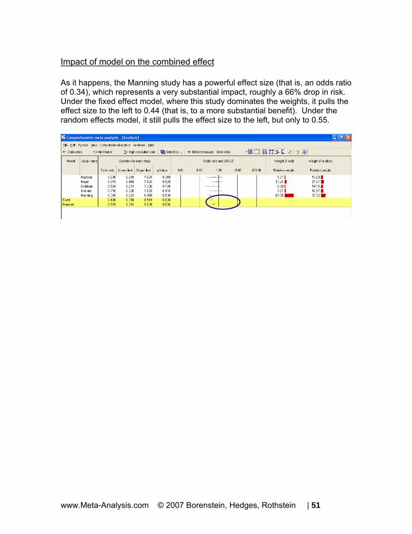
Impact of model on the combined effect As it happens, the Manning study has a powerful effect size (that is, an odds ratio of 0.34), which represents a very substantial impact, roughly a 66% drop in risk. Under the fixed effect model, where this study dominates the weights, it pulls the effect size to the left to 0.44 (that is, to a more substantial benefit). Under the random effects model, it still pulls the effect size to the left, but only to 0.55.
www.Meta-Analysis.com © 2007 Borenstein, Hedges, Rothstein | 51

Impact of model on the confidence interval Under fixed effect, we “set” the between-studies dispersion to zero. Therefore, for the purpose of estimating the mean effect, the only source of uncertainty is within-study error. With a combined total near 1500 subjects per group the within-study error is small, so we have a precise estimate of the combined effect. The confidence interval is relatively narrow, extending from 0.35 to 0.55. Under random effects, dispersion between studies is considered a real source of uncertainty. And, there is a lot of it. The fact that these five studies vary so much one from the other tells us that the effect will vary depending on details that vary randomly from study to study. If the persons who performed these studies happened to use older subjects, or a shorter duration, for example, the effect size would have changed. While this dispersion is “real” in the sense that it is caused by real differences among the studies, it nevertheless represents error if our goal is to estimate the mean effect. For computational purposes, the variance due to between-study differences is included in the error term. In our example we have only five studies, and the effect sizes do vary. Therefore, our estimate of the mean effect is not terribly precise, as reflected in the width of the confidence interval, 0.35 to 0.84, substantially wider than that for the fixed effect model.
www.Meta-Analysis.com © 2007 Borenstein, Hedges, Rothstein | 52
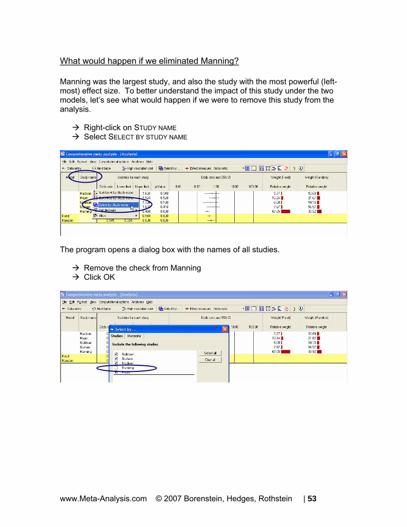
What would happen if we eliminated Manning? Manning was the largest study, and also the study with the most powerful (left-most) effect size. To better understand the impact of this study under the two models, let’s see what would happen if we were to remove this study from the analysis.
Right-click on STUDY NAME Select SELECT BY STUDY NAME
The program opens a dialog box with the names of all studies.
Remove the check from Manning Click OK
www.Meta-Analysis.com © 2007 Borenstein, Hedges, Rothstein | 53

The analysis now looks like this.
For both the fixed effect and random effects models, the combined effect is now close to 0.70.
• Under fixed effects Manning had pulled the effect down to 0.44 • Under random effects Manning had pulled the effect down to 0.55 • Thus, this study had a substantial impact under either model, but more so
under fixed than random effects
Right-click on STUDY NAME Add a check for Manning so the analysis again has five studies
www.Meta-Analysis.com © 2007 Borenstein, Hedges, Rothstein | 54

Additional statistics
Click NEXT TABLE on the toolbar
The program switches to this screen. The program shows the point estimate and confidence interval. These are the same values that had been shown on the forest plot.
• Under fixed effect the combined effect is 0.438 with 95% confidence interval of 0.350 to 0.549
• Under random effects the combined effect is 0.545 with 95% confidence interval of 0.354 to 0.838
www.Meta-Analysis.com © 2007 Borenstein, Hedges, Rothstein | 55

Test of the null hypothesis Under the fixed effect model the null hypothesis is that the common effect is zero. Under the random effects model the null hypothesis is that the mean of the true effects is zero. In either case, the null hypothesis is tested by the z-value, which is computed as Log odds ratio/SE for the corresponding model. To this point we’ve been displaying the odds ratio. The z-value is correct as displayed (since it is always based on the log), but to understand the computation we need to switch the display to show log values. Select LOG ODDS RATIO from the drop down box.
The screen should look like this.
Note that all values are now in log units.
• The point estimate for the fixed effect and random effects models are now -0.825 and -0.607, which are the natural logs of 0.438 and 0.545
• The program now displays the standard error and variance, which can be displayed for the log odds ratio but not for the odds ratio
www.Meta-Analysis.com © 2007 Borenstein, Hedges, Rothstein | 56

For the fixed effect model
−= = −
0.825 7.1520.115
Z
For the random effects model
∗ −= = −
0.607 2.7610.220
Z
With two-tailed p-values < 0.001 and 0.006 respectively.
www.Meta-Analysis.com © 2007 Borenstein, Hedges, Rothstein | 57

Test of the heterogeneity Switch the display back to Odds ratio.
Select ODDS RATIO from the drop-down box
Note, however, that the statistics addressed in this section are always computed using log value, regardless of whether Odds ratio or Log odds ratio has been selected as the index. The null hypothesis for heterogeneity is that the studies share a common effect size. The statistics in this section address the question of whether the observed dispersion among effects exceeds the amount that would be expected by chance.
The Q statistic reflects the observed dispersion. Under the null hypothesis that all studies share a common effect size, the expected value of Q is equal to the degrees of freedom (the number of studies minus 1), and is distributed as Chi-square with df = k-1 (where k is the number of studies).
• The Q statistic is 8.796, as compared with an expected value of 4
www.Meta-Analysis.com © 2007 Borenstein, Hedges, Rothstein | 58

• The p-value is 0.066 If we elect to set alpha at 0.10, then this p-value meets the criterion for statistical significance. If we elect to set alpha at 0.05, then this p-value just misses the criterion. This, of course, is one of the hazards of significance tests. It seems clear that there is substantial dispersion, and probably more than we would expect based on random differences. There probably is real variance among the effects. As discussed in the text, the decision to use a random effects model should be based on our understanding of how the studies were acquired, and should not depend on a statistically significant p-value for heterogeneity. In any event, this p-value does suggest that a fixed effect model does not fit the data.
www.Meta-Analysis.com © 2007 Borenstein, Hedges, Rothstein | 59

Quantifying the heterogeneity While Q is meant to test the null hypothesis that there is no dispersion across effect sizes, we want also to quantify this dispersion. For this purpose we would turn to I-squared and tau-squared.
To see these statistics, scroll the screen toward the right
• I-squared is 54.5, which means that 55% of the observed variance between studies is due to real differences in the effect size. Only about 45% of the observed variance would have been expected based on random error.
• Tau-squared is 0.123. This is the “Between studies” variance that was
used in computing weights. The Q statistic and tau-squared are reported on the fixed effect line, and not on the random effects line. These values are displayed on the fixed effect line because they are computed using fixed effect weights. These values are used in both fixed and random effects analyses, but for different purposes. For the fixed effect analysis Q addresses the question of whether or not the fixed effect model fits the data (is it reasonable to assume that tau-squared is actually zero). However, tau-squared is actually set to zero for the purpose of assigning weights. For the random effects analysis, these values are actually used to assign the weights.
www.Meta-Analysis.com © 2007 Borenstein, Hedges, Rothstein | 60

Return to the main analysis screen Click NEXT TABLE again to get back to the other screen
Your screen should look like this.
www.Meta-Analysis.com © 2007 Borenstein, Hedges, Rothstein | 61

High-resolution plots To this point we’ve used bar graphs to show the weight assigned to each study. Now, we’ll switch to a high-resolution plot, where the weight assigned to each study will determine the size of the symbol representing that study.
Select BOTH MODELS at the bottom of the screen Unclick the SHOW WEIGHTS button on the toolbar Click HIGH RESOLUTION PLOT on the toolbar
www.Meta-Analysis.com © 2007 Borenstein, Hedges, Rothstein | 62

The program shows this screen.
Select COMPUTATIONAL OPTIONS > FIXED EFFECT
Select COMPUTATIONAL OPTIONS > RANDOM EFFECTS
www.Meta-Analysis.com © 2007 Borenstein, Hedges, Rothstein | 63

Compare the weights. In the first plot, using fixed effect weights, the area of the Manning box is about 10 times that of Madison. In the second, using random effects weights, the area of the Manning box is only about 30% larger than Madison.
www.Meta-Analysis.com © 2007 Borenstein, Hedges, Rothstein | 64

Compare the combined effects and standard error.
In the first case (fixed), Manning is given substantial weight and pulls the combined effect left to 0.438. In the second case (random), Manning is given less weight, and the combined effect is 0.545.
www.Meta-Analysis.com © 2007 Borenstein, Hedges, Rothstein | 65

In the first case (fixed) the only source of error is the error within studies and the confidence interval about the combined effect is relatively narrow. In the second case (random) the fact that the true effect varies from study to study introduces another level of uncertainty to our estimate. The confidence interval about the combined effect is substantially wider than it is for the fixed effect analysis.
Click FILE > RETURN TO TABLE
The program returns to the main analysis screen.
www.Meta-Analysis.com © 2007 Borenstein, Hedges, Rothstein | 66

Computational details The program allows you to view details of the computations. Since all calculations are performed using log values, they are easier to follow if we switch the screen to use the log odds ratio as the effect size index.
Select LOG ODDS RATIO from the drop-down box
• The program is now showing the effect for each study and the combined effect using log values
We want to add columns to display the standard error and variance.
Right-click on any of the columns in the STATISTICS FOR EACH STUDY section
Select CUSTOMIZE BASIC STATS
www.Meta-Analysis.com © 2007 Borenstein, Hedges, Rothstein | 67

Check the box next to each statistic Click OK
The screen should look like this.
• Note that we now have columns for the standard error and variance, and all values are in log units
www.Meta-Analysis.com © 2007 Borenstein, Hedges, Rothstein | 68

Computational details for the fixed effect analysis
Select FORMAT > INCREASE DECIMALS on the menu This has no effect on the computations, which are always performed using all significant digits, but it makes the example easier to follow.
On the bottom of the screen select FIXED On the bottom of the screen select CALCULATIONS
www.Meta-Analysis.com © 2007 Borenstein, Hedges, Rothstein | 69

The program switches to this display.
For the first study, Madison
8 * 88LogOddsRatio = Ln = -0.449992 * 12
⎛ ⎞⎜ ⎟⎝ ⎠
1 1 1 1LogOddsVariance = = 0.23068 92 12 88
⎛ ⎞+ + +⎜ ⎟⎝ ⎠
The weight is computed as
11 4.3371
0.2306 0.0000w = =
+
Where the second term in the denominator represents tau-squared, which has been set to zero for the fixed effect analysis. 1 1 ( .4499)(4.3371) 1.9514T w = − = − and so on for the other studies. Then, working with the sums (in the last row)
62.0185 0.824975.1857
T•
−= = −
1 0.013375.1857
v• = =
( ) 0.0133 0.1153SE T• = =
www.Meta-Analysis.com © 2007 Borenstein, Hedges, Rothstein | 70
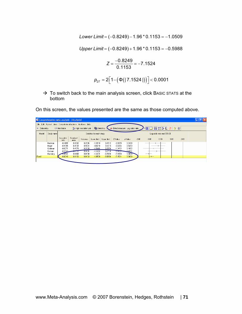
= − − = −( 0.8249) 1.96 * 0.1153 1.0509Lower Limit = − + = −( 0.8249) 1.96 * 0.1153 0.5988Upper Limit
0.8249 7.15240.1153
Z −= = −
( )( )⎡ ⎤= − <⎣ ⎦2 2 1 Φ | 7.1524 | 0.0001Tp
To switch back to the main analysis screen, click BASIC STATS at the bottom
On this screen, the values presented are the same as those computed above.
www.Meta-Analysis.com © 2007 Borenstein, Hedges, Rothstein | 71

Finally, if we select Odds ratio as the index, the program takes the effect size and confidence interval, and displays them as odds ratios.
Concretely, ( )exp 0.8249 0.4383T• = − =
( )exp 1.0509 0.3493Lower Limit = − =
( )= − =exp 0.5988 0.5495Upper Limit The columns for variance and standard error are hidden. The z-value and p-value that had been computed using log values apply here as well, and are displayed without modification.
www.Meta-Analysis.com © 2007 Borenstein, Hedges, Rothstein | 72
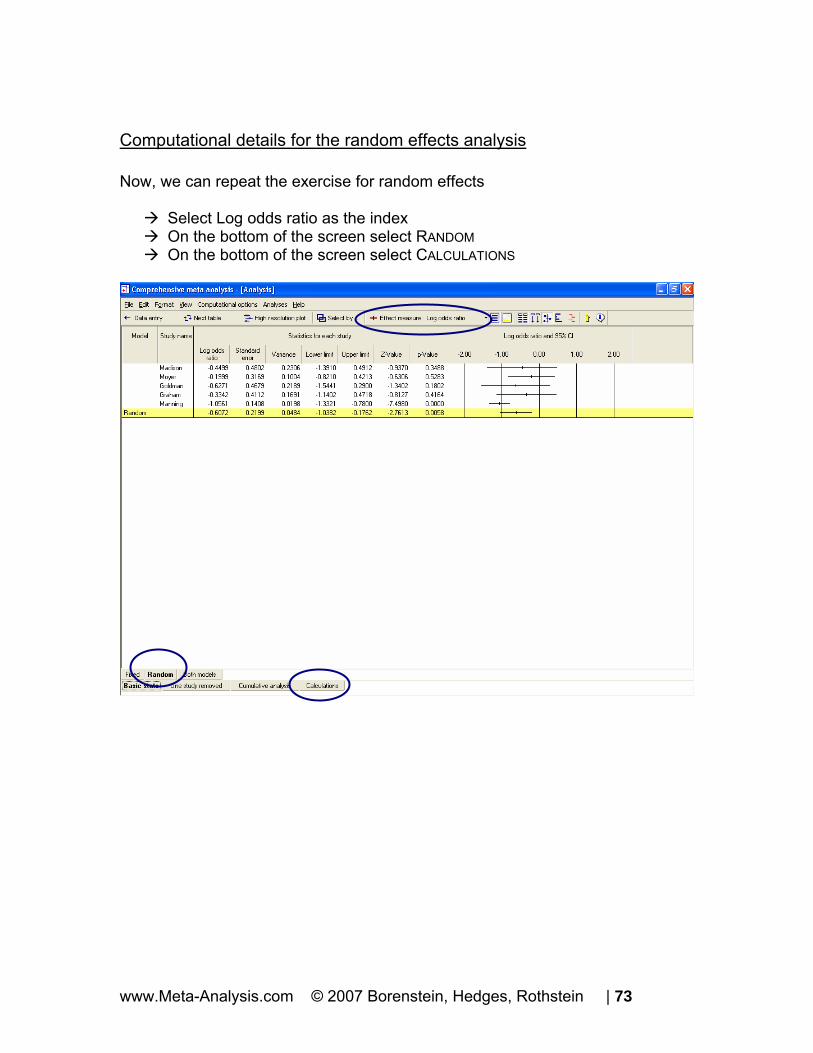
Computational details for the random effects analysis Now, we can repeat the exercise for random effects
Select Log odds ratio as the index On the bottom of the screen select RANDOM On the bottom of the screen select CALCULATIONS
www.Meta-Analysis.com © 2007 Borenstein, Hedges, Rothstein | 73

The program switches to this display.
For the first study, Madison
8 * 88LogOddsRatio = Ln = -0.449992 * 12
⎛ ⎞⎜ ⎟⎝ ⎠
1 1 1 1LogOddsVariance = = 0.23068 92 12 88
⎛ ⎞+ + +⎜ ⎟⎝ ⎠
The weight is computed as
∗ = = =+11 1 2.8305
0.2306 0.1227 0.3533w
Where the (*) indicates that we are using random effects weights, and the second term in the denominator represents tau-squared. ∗ ∗ = − = −1 1 ( 0.4499)(2.8305) 1.2735T w and so on for the other studies. Then, working with the sums (in the last row)
12.5569 0.607220.6791
T ∗•
−= = −
1 0.048420.6791
v ∗• = =
( ) 0.0484 0.2199SE T ∗
• = =
www.Meta-Analysis.com © 2007 Borenstein, Hedges, Rothstein | 74
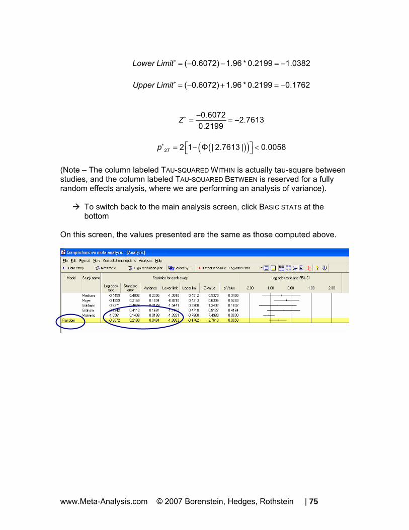
∗ = − − = −( 0.6072) 1.96 * 0.2199 1.0382Lower Limit ∗ = − + = −( 0.6072) 1.96 * 0.2199 0.1762Upper Limit
0.6072 2.76130.2199
Z∗ −= = −
( )( )∗ ⎡ ⎤= − <⎣ ⎦2 2 1 Φ | 2.7613 | 0.0058Tp
(Note – The column labeled TAU-SQUARED WITHIN is actually tau-square between studies, and the column labeled TAU-SQUARED BETWEEN is reserved for a fully random effects analysis, where we are performing an analysis of variance).
To switch back to the main analysis screen, click BASIC STATS at the bottom
On this screen, the values presented are the same as those computed above.
www.Meta-Analysis.com © 2007 Borenstein, Hedges, Rothstein | 75

Finally, if we select Odds ratio as the index, the program takes the effect size and confidence interval, and displays them as odds ratios. The columns for variance and standard error are then hidden.
Concretely, ( )exp 0.6072 0.5449T ∗
• = − =
( )exp 1.0382 .3541Lower Limit ∗ = − =
( )exp 0.1762 0.8384Lower Limit ∗ = − = The columns for variance and standard error are hidden. The z-value and p-value that had been computed using log values apply here as well, and are displayed without modification. This is the conclusion of the exercise for binary data.
www.Meta-Analysis.com © 2007 Borenstein, Hedges, Rothstein | 76

Example 2 ─ Means This appendix shows how to use Comprehensive Meta-Analysis (CMA) to perform a meta-analysis for means using fixed and random effects models. To download a free trial copy of CMA go to www.Meta-Analysis.com If your trial copy has expired, simply ask for a free extension
• Start the program • Click “I want to get an unlock code”, to create an e-mail • In the e-mail, ask for an extension • We’ll send a code by return e-mail
www.Meta-Analysis.com © 2007 Borenstein, Hedges, Rothstein | 77

Start the program and enter the data
Start CMA The program shows this dialog box.
Select START A BLANK SPREADSHEET Click OK
www.Meta-Analysis.com © 2007 Borenstein, Hedges, Rothstein | 78

The program displays this screen.
Insert column for study names
Click INSERT > COLUMN FOR > STUDY NAMES
The program has added a column for Study names.
www.Meta-Analysis.com © 2007 Borenstein, Hedges, Rothstein | 79

Insert columns for the effect size data Since CMA will accept data in more than 100 formats, you need to tell the program what format you want to use. You do have the option to use a different format for each study, but for now we’ll start with one format.
Click INSERT > COLUMN FOR > EFFECT SIZE DATA
The program shows this dialog box.
Click NEXT
www.Meta-Analysis.com © 2007 Borenstein, Hedges, Rothstein | 80

The dialog box lists four sets of effect sizes.
Select COMPARISON OF TWO GROUPS, TIME-POINTS, OR EXPOSURES (INCLUDES CORRELATIONS
Click NEXT
www.Meta-Analysis.com © 2007 Borenstein, Hedges, Rothstein | 81

The program displays this dialog box.
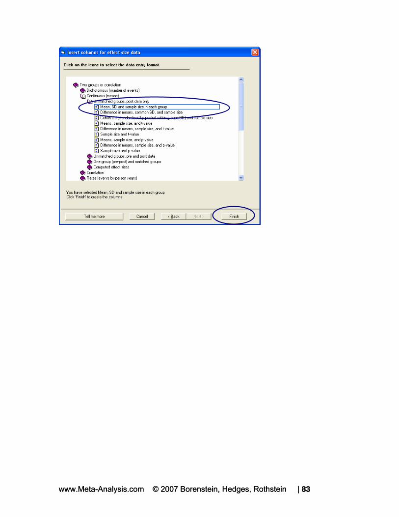
Drill down to
CONTINUOUS (MEANS) UNMATCHED GROUPS, POST DATA ONLY MEAN, SD AND SAMPLE SIZE IN EACH GROUP
Click FINISH
www.Meta-Analysis.com © 2007 Borenstein, Hedges, Rothstein | 82
www.Meta-Analysis.com © 2007 Borenstein, Hedges, Rothstein | 83 www.Meta-Analysis.com © 2007 Borenstein, Hedges, Rothstein | 83

The program will return to the main data-entry screen. The program displays a dialog box that you can use to name the groups.
Enter the names TREATED and CONTROL Click OK
www.Meta-Analysis.com © 2007 Borenstein, Hedges, Rothstein | 84

The program displays the columns needed for the selected format (Means and standard deviations). It also labels these columns using the names Treated and Control. You will enter data into the white columns (at left). The program will compute the effect size for each study and display that effect size in the yellow columns (at right). Since you elected to enter means and SDs the program initially displays columns for the standardized mean difference (Cohen’s d), the bias-corrected standardized mean difference (Hedges’s G) and the raw mean difference. You can add other indices as well.
www.Meta-Analysis.com © 2007 Borenstein, Hedges, Rothstein | 85

Enter the data
Enter the mean, SD, and N for each group as shown here
In the column labeled EFFECT DIRECTION use the drop-down box to select AUTO
(“Auto” means that the program will compute the mean difference as Treated minus Control. You also have the option of selecting “Positive”, in which case the program will assign a plus sign to the difference, or “Negative” in which case it will assign a minus sign to the difference.) The program will automatically compute the effects as shown here in the yellow columns.
www.Meta-Analysis.com © 2007 Borenstein, Hedges, Rothstein | 86

Show details for the computations
Double click on the value 0.540
The program shows how this value was computed.
www.Meta-Analysis.com © 2007 Borenstein, Hedges, Rothstein | 87

Set the default index to Hedges’s G At this point, the program has displayed three indices of effect size – Cohen’s d, Hedges’s G, and the raw mean difference. You have the option of adding additional indices, and/or specifying which index should be used as the “Default” index when you run the analysis.
Right-click on the column for Hedges’s G Click SET PRIMARY INDEX TO HEDGES’S G
www.Meta-Analysis.com © 2007 Borenstein, Hedges, Rothstein | 88

Run the analysis
Click RUN ANALYSES
The program displays this screen.
The default effect size is Hedges’s G The default model is fixed effect
www.Meta-Analysis.com © 2007 Borenstein, Hedges, Rothstein | 89

The screen should look like this.
We can immediately get a sense of the studies and the combined effect. For example,
• All the effects fall on the positive side of zero, in the range of 0.205 to 0.763
• Some studies are clearly more precise than others. The confidence interval for Graham is about four times as wide as the one for Manning, with the other three studies falling somewhere in between
• The combined effect is 0.307 with a 95% confidence interval of 0.234 to 0.380
www.Meta-Analysis.com © 2007 Borenstein, Hedges, Rothstein | 90
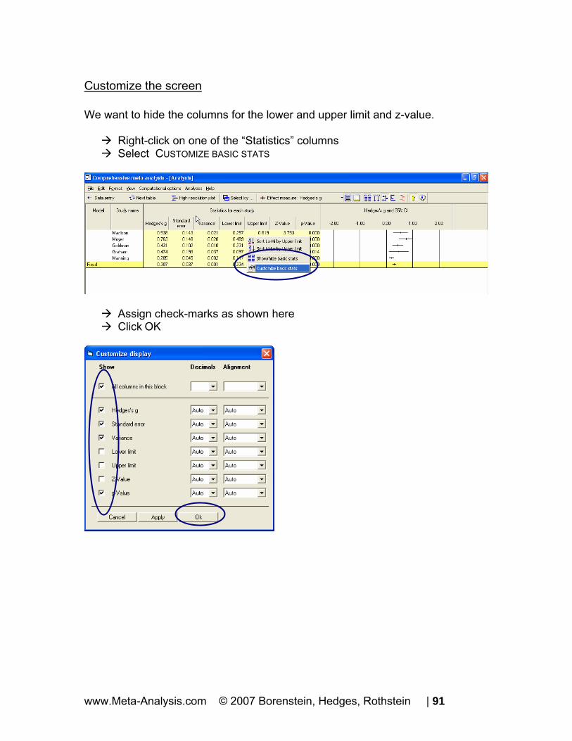
Customize the screen We want to hide the columns for the lower and upper limit and z-value.
Right-click on one of the “Statistics” columns Select CUSTOMIZE BASIC STATS
Assign check-marks as shown here Click OK
www.Meta-Analysis.com © 2007 Borenstein, Hedges, Rothstein | 91

The program has hidden some of the columns, leaving us more room to work with on the display.
Display weights
Click the tool for SHOW WEIGHTS
The program now shows the relative weight assigned to each study for the fixed effect analysis. By “relative weight” we mean the weights as a percentage of the total weights, with all relative weights summing to 100%. For example, Madison was assigned a relative weight of 6.75% while Manning was assigned a relative weight of 69.13%.
www.Meta-Analysis.com © 2007 Borenstein, Hedges, Rothstein | 92

Compare the fixed effect and random effects models
At the bottom of the screen, select BOTH MODELS
• The program shows the combined effect and standard error for both fixed and random effects models
• The program shows weights for both the fixed effect and the random effects models
www.Meta-Analysis.com © 2007 Borenstein, Hedges, Rothstein | 93

Impact of model on study weights The Manning study, with a large sample size (N=1000 per group) is assigned 69% of the weight under the fixed effect model but only 26% of the weight under the random effects model. This follows from the logic of fixed and random effects models explained earlier. Under the fixed effect model we assume that all studies are estimating the same value and this study yields a better estimate than the others, so we take advantage of that. Under the random effects model we assume that each study is estimating a unique effect. The Manning study yields a precise estimate of its population, but that population is only one of many, and we don’t want it to dominate the analysis. Therefore, we assign it 26% of the weight. This is more than the other studies, but not the dominant weight that we gave it under fixed effects.
www.Meta-Analysis.com © 2007 Borenstein, Hedges, Rothstein | 94

Impact of model on the combined effect As it happens, the Manning study has a low effect size. Under the fixed effect model, where this study dominates the weights, it pulls the effect size down to 0.31. Under the random effects model, it still pulls the effect size down, but only to 0.46.
www.Meta-Analysis.com © 2007 Borenstein, Hedges, Rothstein | 95

Impact of model on the confidence interval Under fixed effect, we “set” the between-studies dispersion to zero. Therefore, for the purpose of estimating the mean effect, the only source of uncertainty is within-study error. With a combined total near 1500 subjects per group the within-study error is small, so we have a precise estimate of the combined effect. The standard error is 0.037. Under random effects, dispersion between studies is considered a real source of uncertainty. And, there is a lot of it. The fact that these five studies vary so much one from the other tells us that the effect will vary depending on details that vary randomly from study to study. If the persons who performed these studies happened to use older subjects, or a shorter duration, for example, the effect size would have changed. While this dispersion is “real” in the sense that it is caused by real differences among the studies, it nevertheless represents error if our goal is to estimate the mean effect. For computational purposes, the variance due to between-study differences is included in the error term. In our example we have only five studies, and the effect sizes do vary. Therefore, our estimate of the mean effect is not terribly precise, as reflected in a standard error of 0.112, which is about three times that of the fixed effect value.
www.Meta-Analysis.com © 2007 Borenstein, Hedges, Rothstein | 96

What would happen if we eliminated Manning? Manning was the largest study, and also the study with the smallest effect size. To better understand the impact of this study under the two models, let’s see what would happen if we were to remove this study from the analysis.
Right-click on STUDY NAME Select SELECT BY STUDY NAME
The program opens a dialog box with the names of all studies.
Remove the check from Manning Click OK
www.Meta-Analysis.com © 2007 Borenstein, Hedges, Rothstein | 97

The analysis now looks like this.
For both the fixed effect and random effects models, the combined effect is now close to 0.54.
• Under fixed effects Manning had pulled the effect down to 0.31 • Under random effects Manning had pulled the effect down to 0.46 • Thus, this study had a substantial impact under either model, but more so
under fixed than random effects
Right-click on STUDY NAME Add a check for Manning so the analysis again has five studies
www.Meta-Analysis.com © 2007 Borenstein, Hedges, Rothstein | 98
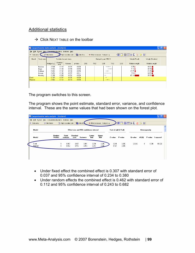
Additional statistics
Click NEXT TABLE on the toolbar
The program switches to this screen. The program shows the point estimate, standard error, variance, and confidence interval. These are the same values that had been shown on the forest plot.
• Under fixed effect the combined effect is 0.307 with standard error of 0.037 and 95% confidence interval of 0.234 to 0.380
• Under random effects the combined effect is 0.462 with standard error of 0.112 and 95% confidence interval of 0.243 to 0.682
www.Meta-Analysis.com © 2007 Borenstein, Hedges, Rothstein | 99

Test of the null hypothesis Under the fixed effect model the null hypothesis is that the common effect is zero. Under the random effects model the null hypothesis is that the mean of the true effects is zero. In either case, the null hypothesis is tested by the z-value, which is computed as G/SE for the corresponding model.
For the fixed effect model
.307Z= =8.244.037
For the random effects model
∗ 0.462Z = =4.1270.112
In either case, the two-tailed p-value is < 0.001.
www.Meta-Analysis.com © 2007 Borenstein, Hedges, Rothstein | 100

Test of the heterogeneity The null hypothesis for heterogeneity is that the studies share a common effect size. The statistics in this section address the question of whether the observed dispersion among effects exceeds the amount that would be expected by chance.
The Q statistic reflects the observed dispersion. Under the null hypothesis that all studies share a common effect size, the expected value of Q is equal to the degrees of freedom (the number of studies minus 1), and is distributed as Chi-square with df = k-1 (where k is the number of studies).
• The Q statistic is 20.64, as compared with an expected value of 4 • The p-value is < 0.001
As discussed in the text, the decision to use a random effects model should be based on our understanding of how the studies were acquired, and should not depend on a statistically significant p-value for heterogeneity. In any event, however, this p-value tells us that the observed dispersion cannot be attributed to random error, and there is real variance among the effects. A fixed effect model would not fit the data.
www.Meta-Analysis.com © 2007 Borenstein, Hedges, Rothstein | 101

Quantifying the heterogeneity While Q is meant to test the null hypothesis that there is no dispersion across effect sizes, we want also to quantify this dispersion. For this purpose we would turn to I-squared and tau-squared.
To see these statistics, scroll the screen toward the right
• I-squared is 80.6, which means that 80% of the observed variance between studies is due to real differences in the effect size. Only about 20% of the observed variance would have been expected based on random error.
• Tau-squared is 0.047. This is the “Between studies” variance that was
used in computing weights. The Q statistic and tau-squared are reported on the fixed effect line, and not on the random effects line. These values are displayed on the fixed effect line because they are computed using fixed effect weights. These values are used in both fixed and random effects analyses, but for different purposes. For the fixed effect analysis Q addresses the question of whether or not the fixed effect model fits the data (is it reasonable to assume that tau-squared is actually zero). However, tau-squared is actually set to zero for the purpose of assigning weights. For the random effects analysis, these values are actually used to assign the weights.
www.Meta-Analysis.com © 2007 Borenstein, Hedges, Rothstein | 102

Return to the main analysis screen Click NEXT TABLE again to get back to the other screen.
Your screen should look like this.
www.Meta-Analysis.com © 2007 Borenstein, Hedges, Rothstein | 103

High-resolution plots To this point we’ve used bar graphs to show the weight assigned to each study. Now, we’ll switch to a high-resolution plot, where the weight assigned to each study will determine the size of the symbol representing that study.
Select BOTH MODELS at the bottom of the screen Unclick the SHOW WEIGHTS button on the toolbar Click HIGH-RESOLUTION PLOT on the toolbar
www.Meta-Analysis.com © 2007 Borenstein, Hedges, Rothstein | 104

The program shows this screen.
Select COMPUTATIONAL OPTIONS > FIXED EFFECT
Select COMPUTATIONAL OPTIONS > RANDOM EFFECTS
www.Meta-Analysis.com © 2007 Borenstein, Hedges, Rothstein | 105

Compare the weights. In the first plot, using fixed effect weights, the area of the Manning box is about 10 times that of Madison. In the second, using random effects weights, the area of the Manning box is only about 30% larger than Madison.
www.Meta-Analysis.com © 2007 Borenstein, Hedges, Rothstein | 106

Compare the combined effects and standard error.
In the first case (fixed) Manning is given substantial weight and pulls the combined effect down to 0.307. In the second case (random) Manning is given less weight, and the combined effect is 0.462. In the first case (fixed) the only source of error is the error within studies. The standard error of the combined effect is 0.037 and the confidence interval about the combined effect is relatively narrow. In the second case (random) the fact that the true effect varies from study to study introduces another level of uncertainty to our estimate. The standard error of the combined effect is 0.112,
www.Meta-Analysis.com © 2007 Borenstein, Hedges, Rothstein | 107

and the confidence interval about the combined effect is about three times as wide as that for the fixed effect analysis.
Click FILE > RETURN TO TABLE
The program returns to the main analysis screen.
www.Meta-Analysis.com © 2007 Borenstein, Hedges, Rothstein | 108

Computational details The program allows you to view details of the computations.
Computational details for the fixed effect analysis
Select FORMAT > INCREASE DECIMALS on the menu This has no effect on the computations, which are always performed using all significant digits, but it makes the example easier to follow.
On the bottom of the screen select FIXED On the bottom of the screen select CALCULATIONS
www.Meta-Analysis.com © 2007 Borenstein, Hedges, Rothstein | 109

The program switches to this display.
For the first study, Madison RawDifference =410-360=50
( ) ( )+
=+ −
2 2
Pooled
(100-1)(90 ) (100-1)(95 )SD = 92.534
100 100 2
= =50 0.5403
92.534d
= + + =+
21 1 0.5403 0.1440100 100 2 * (100 100)dSE
⎛ ⎞ =⎜ ⎟⎝ ⎠
3J = 1 - 0.9964 * 198 - 1
= =0.996 * 0.5403 0.5383G = =0.996 * 0.1440 0.1434GSE = =2 20.1434 0.0206GSE The weight is computed as
11 48.6074
0.0206 0.0000w = =
+
www.Meta-Analysis.com © 2007 Borenstein, Hedges, Rothstein | 110

where the second term in the denominator represents tau-squared, which has been set to zero for the fixed effect analysis. = =1 1 0.5383 * 48.6074 26.1651T w and so on for the other studies. Then, working with the sums (in the last row)
• = =221.2233 0.3072720.0528
T
1 0.0014720.0528
v• = =
( ) 0.0014 0.0373SE T• = = = − =0.3072 1.96 * 0.0373 0.2342Lower Limit = + =0.3072 1.96 * 0.0373 0.3803Upper Limit
= =0.3072 8.24420.0373
Z
( )( )⎡ ⎤= − <⎣ ⎦2 2 1 Φ | 8.2242 | 0.0001Tp
www.Meta-Analysis.com © 2007 Borenstein, Hedges, Rothstein | 111

To switch back to the main analysis screen, click BASIC STATS at the bottom
These are the same values presented here
www.Meta-Analysis.com © 2007 Borenstein, Hedges, Rothstein | 112

Computational details for the random effects analysis Now, we can repeat the exercise for random effects.
On the bottom of the screen select RANDOM On the bottom of the screen select CALCULATIONS
www.Meta-Analysis.com © 2007 Borenstein, Hedges, Rothstein | 113

The program switches to this display.
For the first study, Madison RawDifference =410-360=50
( ) ( )+
=+ −
2 2
Pooled
(100-1)(90 ) (100-1)(95 )SD = 92.534
100 100 2
50 0.540392.534
d = =
= + + =+
21 1 0.5403 0.1440100 100 2 * (100 100)dSE
⎛ ⎞ =⎜ ⎟⎝ ⎠
3J = 1 - 0.9964 * 198 - 1
= =0.996 * 0.5403 0.5383G = =0.996 * 0.1440 0.1434GSE = =2 20.1434 .0206GSE The weight is computed as
∗ = = =+11 1 14.8356
0.0206 0.0468 0.0674w
www.Meta-Analysis.com © 2007 Borenstein, Hedges, Rothstein | 114

where the (*) indicates that we are using random effects weights, and the second term in the denominator represents tau-squared. ∗ ∗ = =1 1 0.5383 *14.8356 7.9859T w and so on for the other studies. Then, working with the sums (in the last row)
∗• = =
36.8481 0.462179.7353
T
1 0.012579.7353
v ∗• = =
( ) 0.0125 0.1120SE T ∗
• = = ∗ = − =0.4621 1.96 * 0.1120 0.2426Lower Limit ∗ = + =0.4621 1.96 * 0.1120 0.6816Upper Limit
∗ = =0.4621 4.12660.1120
Z
( )( )∗ ⎡ ⎤= − <⎣ ⎦2 2 1 Φ | 4.1266 | 0.0001Tp
(Note – The column labeled TAU-SQUARED WITHIN is actually tau-squared between studies, and the column labeled TAU-SQUARED BETWEEN is reserved for a fully random effects analysis, where we are performing an analysis of variance).
To switch back to the main analysis screen, click BASIC STATS at the bottom
On this screen, the values presented are the same as those computed above.
www.Meta-Analysis.com © 2007 Borenstein, Hedges, Rothstein | 115

This is the conclusion of the exercise for means.
www.Meta-Analysis.com © 2007 Borenstein, Hedges, Rothstein | 116
Example 3 ─ Correlational Data This appendix shows how to use Comprehensive Meta-Analysis (CMA) to perform a meta-analysis for correlations using fixed and random effects models. To download a free trial copy of CMA go to www.Meta-Analysis.com If your trial copy has expired, simply ask for a free extension
• Start the program • Click “I want to get an unlock code”, to create an e-mail • In the e-mail, ask for an extension • We’ll send a code by return e-mail
www.Meta-Analysis.com © 2007 Borenstein, Hedges, Rothstein | 117

Start the program and enter the data
Start CMA The program shows this dialog box.
Select START A BLANK SPREADSHEET Click OK
www.Meta-Analysis.com © 2007 Borenstein, Hedges, Rothstein | 118

The program displays this screen.
Insert column for study names
Click INSERT > COLUMN FOR > STUDY NAMES
The program has added a column for Study names.
www.Meta-Analysis.com © 2007 Borenstein, Hedges, Rothstein | 119

Insert columns for the effect size data Since CMA will accept data in more than 100 formats, you need to tell the program what format you want to use. You do have the option to use a different format for each study, but for now we’ll start with one format.
Click INSERT > COLUMN FOR > EFFECT SIZE DATA
The program shows this dialog box
Click NEXT
www.Meta-Analysis.com © 2007 Borenstein, Hedges, Rothstein | 120
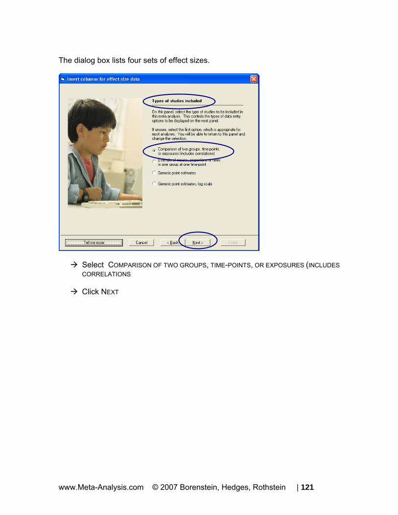
The dialog box lists four sets of effect sizes.
Select COMPARISON OF TWO GROUPS, TIME-POINTS, OR EXPOSURES (INCLUDES CORRELATIONS
Click NEXT
www.Meta-Analysis.com © 2007 Borenstein, Hedges, Rothstein | 121

The program displays this dialog box.
Drill down to
CORRELATION COMPUTED EFFECT SIZES CORRELATION AND SAMPLE SIZE
Click FINISH
www.Meta-Analysis.com © 2007 Borenstein, Hedges, Rothstein | 122

www.Meta-Analysis.com © 2007 Borenstein, Hedges, Rothstein | 123 www.Meta-Analysis.com © 2007 Borenstein, Hedges, Rothstein | 123

The program will return to the main data-entry screen. The program displays the columns needed for the selected format (Correlation, Sample size). You will enter data into the white columns (at left). The program will compute the effect size for each study and display that effect size in the yellow columns (at right). Since you elected work with correlational data the program initially displays columns for the correlation and the Fisher ‘s Z transformation of the correlation. You can add other indices as well.
www.Meta-Analysis.com © 2007 Borenstein, Hedges, Rothstein | 124

Enter the data
Enter the correlation and sample size for each study as shown here
The program will automatically compute the standard error and Fisher’s Z values as shown here in the yellow columns.
www.Meta-Analysis.com © 2007 Borenstein, Hedges, Rothstein | 125

What are Fisher’s Z values The Fisher’s Z value is a transformation of the correlation into a different metric. The standard error of a correlation is a function not only of sample size but also of the correlation itself, with larger correlations (either positive or negative) having a smaller standard error. This can cause problems in a meta-analysis since this would lead the larger correlations to appear more precise and be assigned more weight in the analysis. To avoid this problem we convert all correlations to the Fisher’s Z metric, whose standard error is determined solely by sample size. All computations are performed using Fisher’s Z. The results are then converted back to correlations for display. Fisher’s Z should not be confused with the Z statistic used to test hypotheses. The two are not related. This table shows the correspondence between the correlation value and Fisher’s Z for specific correlations. Note that the two are similar for correlations near zero, but diverge substantially as the correlation increases.
All conversions are handled automatically by the program. That is, if you enter data using correlations, the program will automatically convert these to Fisher’s Z, perform the analysis, and then reconvert the values to correlations for display. The transformation from correlation to Fisher’s Z is given by
10.5 *1
CorrelationFisherZ LogCorrelation
+⎛= ⎜ −⎝ ⎠⎞⎟
www.Meta-Analysis.com © 2007 Borenstein, Hedges, Rothstein | 126

1
3FisherZSEN
=−
The transformation from Fisher’s Z to correlation is given by (2 * )C Exp FisherZ=
11
CCorrelationC−⎛= ⎜
⎞⎟+⎝ ⎠
2(1 ) *Correlation FisherZSE Correlation SE= −
www.Meta-Analysis.com © 2007 Borenstein, Hedges, Rothstein | 127

Show details for the computations.
Double click on the value 0.261
The program shows how all related values were computed.
www.Meta-Analysis.com © 2007 Borenstein, Hedges, Rothstein | 128

Set the default index At this point, the program has displayed the correlation and the Fisher’s Z transformation, which we’ll be using in this example. You have the option of adding additional indices, and/or specifying which index should be used as the “Default” index when you run the analysis.
Right-click on any of the yellow columns Select CUSTOMIZE COMPUTED EFFECT SIZE DISPLAY
www.Meta-Analysis.com © 2007 Borenstein, Hedges, Rothstein | 129

The program displays this dialog box.
You could use this dialog box to add or remove effect size indices from the display.
Click OK
www.Meta-Analysis.com © 2007 Borenstein, Hedges, Rothstein | 130

Run the analysis
Click RUN ANALYSES
The program displays this screen.
The default effect size is the correlation The default model is fixed effect
www.Meta-Analysis.com © 2007 Borenstein, Hedges, Rothstein | 131

The screen should look like this.
We can immediately get a sense of the studies and the combined effect. For example,
• All the correlations are positive, and they all fall in the range of 0.102 to 0.356
• Some studies are clearly more precise than others. The confidence interval for Graham is substantially wider than the one for Manning, with the other three studies falling somewhere in between
• The combined correlation is 0.151 with a 95% confidence interval of 0.115 to 0.186
www.Meta-Analysis.com © 2007 Borenstein, Hedges, Rothstein | 132

Customize the screen We want to hide the column for the z-value.
Right-click on one of the “Statistics” columns Select CUSTOMIZE BASIC STATS
Assign check-marks as shown here Click OK
Note – the standard error and variance are never displayed for the correlation. They are displayed when the corresponding boxes are checked and Fisher’s Z is selected as the index.
www.Meta-Analysis.com © 2007 Borenstein, Hedges, Rothstein | 133

The program has hidden some of the columns, leaving us more room to work with on the display.
Display weights
Click the tool for SHOW WEIGHTS
The program now shows the relative weight assigned to each study for the fixed effect analysis. By “relative weight” we mean the weights as a percentage of the total weights, with all relative weights summing to 100%. For example, Madison was assigned a relative weight of 6.83% while Manning was assigned a relative weight of 69.22%.
www.Meta-Analysis.com © 2007 Borenstein, Hedges, Rothstein | 134

Compare the fixed effect and random effects models
At the bottom of the screen, select BOTH MODELS
• The program shows the combined effect and confidence limits for both fixed and random effects models
• The program shows weights for both the fixed effect and the random effects models
www.Meta-Analysis.com © 2007 Borenstein, Hedges, Rothstein | 135

Impact of model on study weights The Manning study, with a large sample size (N=2000) is assigned 69% of the weight under the fixed effect model, but only 26% of the weight under the random effects model. This follows from the logic of fixed and random effects models explained earlier. Under the fixed effect model we assume that all studies are estimating the same value and this study yields a better estimate than the others, so we take advantage of that. Under the random effects model we assume that each study is estimating a unique effect. The Manning study yields a precise estimate of its population, but that population is only one of many, and we don’t want it to dominate the analysis. Therefore, we assign it 26% of the weight. This is more than the other studies, but not the dominant weight that we gave it under fixed effects.
www.Meta-Analysis.com © 2007 Borenstein, Hedges, Rothstein | 136

Impact of model on the combined effect As it happens, the Manning study of 0.102 is the smallest effect size in this group of studies. Under the fixed effect model, where this study dominates the weights, it pulls the combined effect down to 0.151. Under the random effects model, it still pulls the effect size down, but only to 0.223.
www.Meta-Analysis.com © 2007 Borenstein, Hedges, Rothstein | 137

Impact of model on the confidence interval Under fixed effect, we “set” the between-studies dispersion to zero. Therefore, for the purpose of estimating the mean effect, the only source of uncertainty is within-study error. With a combined total near 3000 subjects the within-study error is small, so we have a precise estimate of the combined effect. The confidence interval is relatively narrow, extending from 0.12 to 0.19. Under random effects, dispersion between studies is considered a real source of uncertainty. And, there is a lot of it. The fact that these five studies vary so much one from the other tells us that the effect will vary depending on details that vary randomly from study to study. If the persons who performed these studies happened to use older subjects, or a shorter duration, for example, the effect size would have changed. While this dispersion is “real” in the sense that it is caused by real differences among the studies, it nevertheless represents error if our goal is to estimate the mean effect. For computational purposes, the variance due to between-study differences is included in the error term. In our example we have only five studies, and the effect sizes do vary. Therefore, our estimate of the mean effect is not terribly precise, as reflected in the width of the confidence interval, 0.12 to 0.32, substantially wider than that for the fixed effect model.
www.Meta-Analysis.com © 2007 Borenstein, Hedges, Rothstein | 138

What would happen if we eliminated Manning? Manning was the largest study, and also the study with the most powerful (left-most) effect size. To better understand the impact of this study under the two models, let’s see what would happen if we were to remove this study from the analysis.
Right-click on STUDY NAME Select SELECT BY STUDY NAME
The program opens a dialog box with the names of all studies.
Remove the check from Manning Click OK
www.Meta-Analysis.com © 2007 Borenstein, Hedges, Rothstein | 139

The analysis now looks like this.
For both the fixed effect and random effects models, the combined effect is now approximately 0.26.
• Under fixed effects Manning had pulled the effect down to 0.15 • Under random effects Manning had pulled the effect down to 0.22 • Thus, this study had a substantial impact under either model, but more so
under fixed than random effects
Right-click on STUDY NAMES Add a check for Manning so the analysis again has five studies
www.Meta-Analysis.com © 2007 Borenstein, Hedges, Rothstein | 140

Additional statistics
Click NEXT TABLE on the toolbar
The program switches to this screen. The program shows the point estimate and confidence interval. These are the same values that had been shown on the forest plot.
• Under fixed effect the combined effect is 0.151 with 95% confidence interval of 0.115 to 0.186
• Under random effects the combined effect is 0.223 with 95% confidence interval of 0.120 to 0.322
www.Meta-Analysis.com © 2007 Borenstein, Hedges, Rothstein | 141

Test of the null hypothesis Under the fixed effect model the null hypothesis is that the common effect is zero. Under the random effects model the null hypothesis is that the mean of the true effects is zero. In either case, the null hypothesis is tested by the z-value, which is computed as Fisher’s Z/SE for the corresponding model. To this point we’ve been displaying the correlation rather than the Fisher’s Z value. The test statistic Z (not to be confused with Fisher’s Z) is correct as displayed (since it is always based on the Fisher’s Z transform), but to understand the computation we need to switch the display to show Fisher’s Z values. Select FISHER’S Z from the drop down box
www.Meta-Analysis.com © 2007 Borenstein, Hedges, Rothstein | 142

The screen should look like this (use the Format menu to display additional decimal places).
Note that all values are now in Fisher’s Z units.
• The point estimate for the fixed effect and random effects models are now 0.152 and 0.227, which are the Fisher’s Z transformations of the correlations, 0.151 and 0.223. (The difference between the correlation and the Fisher’s Z value becomes more pronounced as the size of the correlation increases)
• The program now displays the standard error and variance, which can be displayed for the Fisher’s Z value but not for the correlation
For the fixed effect analysis
= =0.1519 8.16000.0186
Z
For the random effect analysis
= =0.2273 4.17200.0545
Z
In either case, the two-tailed p-value is < 0.0001.
www.Meta-Analysis.com © 2007 Borenstein, Hedges, Rothstein | 143

Test of the heterogeneity Switch the display back to correlation
Select CORRELATION from the drop-down box
Note, however, that the statistics addressed in this section are always computed using the Fisher’s Z values, regardless of whether Correlation or Fisher’s Z has been selected as the index. The null hypothesis for heterogeneity is that the studies share a common effect size. The statistics in this section address the question of whether or the observed dispersion among effects exceeds the amount that would be expected by chance.
www.Meta-Analysis.com © 2007 Borenstein, Hedges, Rothstein | 144

The Q statistic reflects the observed dispersion. Under the null hypothesis that all studies share a common effect size, the expected value of Q is equal to the degrees of freedom (the number of studies minus 1), and is distributed as Chi-square with df = k-1 (where k is the number of studies).
• The Q statistic is 19.3179, as compared with an expected value of 4 • The p-value is 0.0007
This p-value meets the criterion for statistical significance. It seems clear that there is substantial dispersion, and probably more than we would expect based on random differences. There probably is real variance among the effects. As discussed in the text, the decision to use a random effects model should be based on our understanding of how the studies were acquired, and should not depend on a statistically significant p-value for heterogeneity. In any event, this p-value does suggest that a fixed effect model does not fit the data.
www.Meta-Analysis.com © 2007 Borenstein, Hedges, Rothstein | 145

Quantifying the heterogeneity While Q is meant to test the null hypothesis that there is no dispersion across effect sizes, we want also to quantify this dispersion. For this purpose we would turn to I-squared and Tau-squared.
To see these statistics, scroll the screen toward the right
• I-squared is 79.29, which means that 79% of the observed variance between studies is due to real differences in the effect size. Only about 21% of the observed variance would have been expected based on random error.
• Tau-squared is 0.0108. This is the “Between studies” variance that was
used in computing weights. The Q statistic and tau-squared are reported on the fixed effect line, and not on the random effects line. These value are displayed on the fixed effect line because they are computed using fixed effect weights. These values are used in both fixed and random effects analyses, but for different purposes. For the fixed effect analysis Q addresses the question of whether or not the fixed effect model fits the data (is it reasonable to assume that tau-squared is actually zero). However, tau-squared is actually set to zero for the purpose of assigning weights. For the random effects analysis, these values are actually used to assign the weights.
www.Meta-Analysis.com © 2007 Borenstein, Hedges, Rothstein | 146

Return to the main analysis screen Click NEXT TABLE again to get back to the other screen.
Your screen should look like this
www.Meta-Analysis.com © 2007 Borenstein, Hedges, Rothstein | 147

High-resolution plots To this point we’ve used bar graphs to show the weight assigned to each study. Now, we’ll switch to a high-resolution plot, where the weight assigned to each study will be incorporated into the symbol representing that study.
Select BOTH MODELS at the bottom of the screen Unclick the SHOW WEIGHTS button on the toolbar Click HIGH-RESOLUTION PLOT on the toolbar
www.Meta-Analysis.com © 2007 Borenstein, Hedges, Rothstein | 148

The program shows this screen.
Select COMPUTATIONAL OPTIONS > FIXED EFFECT
Select COMPUTATIONAL OPTIONS > RANDOM EFFECTS
www.Meta-Analysis.com © 2007 Borenstein, Hedges, Rothstein | 149

Compare the weights. In the first plot, using fixed effect weights, the area of the Manning box was about 20 times that of Graham. In the second, using random effects weights, the area of the Manning box was only about twice as large as Graham.
www.Meta-Analysis.com © 2007 Borenstein, Hedges, Rothstein | 150
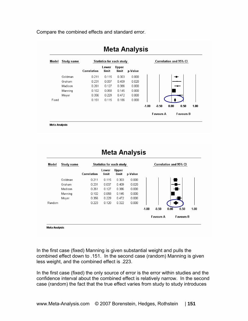
Compare the combined effects and standard error.
In the first case (fixed) Manning is given substantial weight and pulls the combined effect down to .151. In the second case (random) Manning is given less weight, and the combined effect is .223. In the first case (fixed) the only source of error is the error within studies and the confidence interval about the combined effect is relatively narrow. In the second case (random) the fact that the true effect varies from study to study introduces
www.Meta-Analysis.com © 2007 Borenstein, Hedges, Rothstein | 151

another level of uncertainty to our estimate. The confidence interval about the combined effect is substantially wider than it is for the fixed effect analysis.
Click FILE > RETURN TO TABLE
The program returns to the main analysis screen.
www.Meta-Analysis.com © 2007 Borenstein, Hedges, Rothstein | 152

Computational details The program allows you to view details of the computations Since all calculations are performed using Fisher’s Z values, they are easier to follow if we switch the screen to use Fisher’s Z as the effect size index.
Select FISHER’S Z from the drop-down box
• The program is now showing the effect for each study and the combined effect using values in the Fisher’s Z metric.
We want to add columns to display the standard error and variance.
Right-click on any of the columns in the STATISTICS FOR EACH STUDY section
Select CUSTOMIZE BASIC STATS
www.Meta-Analysis.com © 2007 Borenstein, Hedges, Rothstein | 153

Check the box next to each statistic Click OK
The screen should look like this.
• Note that we now have columns for the standard error and variance, and all values are in Fisher’s Z units
www.Meta-Analysis.com © 2007 Borenstein, Hedges, Rothstein | 154
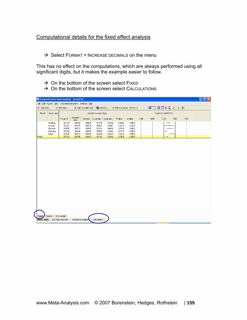
Computational details for the fixed effect analysis
Select FORMAT > INCREASE DECIMALS on the menu This has no effect on the computations, which are always performed using all significant digits, but it makes the example easier to follow.
On the bottom of the screen select FIXED On the bottom of the screen select CALCULATIONS
www.Meta-Analysis.com © 2007 Borenstein, Hedges, Rothstein | 155

The program switches to this display.
For the first study, Madison, the correlation was entered as .261 with a sample size of 200. The program computed the Fisher’s Z value and its variance as follows (to see these computations return to the data entry screen and double-click on the computed value).
1 + 0.2610.5 * Log = 0.2671 - 0.261
FisherZ ⎛ ⎞= ⎜ ⎟⎝ ⎠
1SE= = 0.0712
200-3
= =20.0712 0.0051Variance The weight is computed as
11 197.0000
0.0051 0.0000w = =
+
Where the second term in the denominator represents tau-squared, which has been set to zero for the fixed effect analysis. = =1 1 (0.2670)(197.0000) 52.5967T w and so on for the other studies. Then, working with the sums (in the last row)
• = =438.2894 0.1519
2885.0000T
www.Meta-Analysis.com © 2007 Borenstein, Hedges, Rothstein | 156

• = =1 0.0003
2885.0000v
( ) 0.0003 0.0186SE T• = = = − =0.1519 1.96 * 0.0186 0.1154Lower Limit = + =0.1519 1.96 * 0.0186 0.1884Upper Limit
0.1519 8.16000.0186
Z = =
To switch back to the main analysis screen, click BASIC STATS at the bottom
On this screen, the values presented are the same as those computed above.
www.Meta-Analysis.com © 2007 Borenstein, Hedges, Rothstein | 157

Finally, if we select Correlation as the index, the program takes the effect size and confidence interval, and displays them as correlations.
To transform the combined effect (Fisher’s Z = 0.1519) to a correlation ( )= =exp 2 * 0.1519 1.355C
1.355 1 0.1511.355 1
T•
−= =
+ To transform the lower limit (Fisher’s Z = 0.1154) to a correlation ( )exp 2 * 0.1154 1.260C = =
1.260 1 0.11491.260 1
LowerLimit −= =
+ To transform the upper limit (Fisher’s Z = 0.1884) to a correlation ( )exp 2 * 0.1884 1.458C = =
1.458 1 0.18621.458 1
UpperLimit −= =
+ The columns for variance and standard error are hidden. The z-value and p-value that had been computed using Fisher’s Z values apply here as well, and are displayed without modification.
www.Meta-Analysis.com © 2007 Borenstein, Hedges, Rothstein | 158

Computational details for the random effects analysis Now, we can repeat the exercise for random effects.
Select FISHER’S Z as the index On the bottom of the screen select RANDOM On the bottom of the screen select CALCULATIONS
www.Meta-Analysis.com © 2007 Borenstein, Hedges, Rothstein | 159

The program switches to this display
For the first study, Madison, the correlation was entered as 0.261 with a sample size of 200. The program computed the Fisher’s Z value and its variance as follows (to see these computations return to the data entry screen and double-click on the computed value).
1 + 0.2610.5 * Log = 0.2671 - 0.261
FisherZ ⎛ ⎞= ⎜ ⎟⎝ ⎠
1SE= = 0.0712
200-3
= =20.0712 0.0051Variance The weight is computed as
∗ = = =+11 1 62.9742
0.0051 0.0108 0.0159w
Where the (*) indicates that we are using random effects weights, and the second term in the denominator represents tau-squared. ∗ ∗ = =1 1 (.2670)(62.9742) 16.8134T w and so on for the other studies. Then, working with the sums (in the last row)
www.Meta-Analysis.com © 2007 Borenstein, Hedges, Rothstein | 160
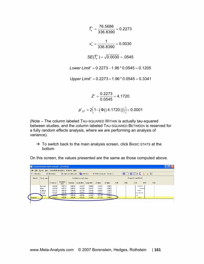
76.5686 0.2273336.8390
T ∗• = =
∗• = =
1 0.0030336.8390
v
( ) 0.0030 .0545SE T ∗
• = = ∗ = − =0.2273 1.96 * 0.0545 0.1205Lower Limit ∗ = + =0.2273 1.96 * 0.0545 0.3341Upper Limit
∗ = =0.2273 4.17200.0545
Z
( )( )∗ ⎡ ⎤= − <⎣ ⎦2 2 1 Φ | 4.1720 | 0.0001Tp
(Note – The column labeled TAU-SQUARED WITHIN is actually tau-squared between studies, and the column labeled TAU-SQUARED BETWEEN is reserved for a fully random effects analysis, where we are performing an analysis of variance).
To switch back to the main analysis screen, click BASIC STATS at the bottom
On this screen, the values presented are the same as those computed above.
www.Meta-Analysis.com © 2007 Borenstein, Hedges, Rothstein | 161

Finally, if we select Correlation as the index, the program takes the effect size and confidence interval, and displays them as correlations. The columns for variance and standard error are then hidden.
To transform the combined effect (Fisher’s Z = 0.2273) to a correlation ( )exp 2 * 0.2273 1.576C = =
1.576 1 0.22351.576 1
T•
−= =
+ To transform the lower limit (Fisher’s Z = 0.1205) to a correlation ( )exp 2 * 0.1205 1.273C = =
1.273 1 0.11991.273 1
LowerLimit −= =
+ To transform the upper limit (Fisher’s Z = 0.3341) to a correlation ( )exp 2 * 0.3341 1.951C = =
1.951 1 0.32221.951 1
UpperLimit −= =
+ The columns for variance and standard error are hidden. The z-value and p-value that had been computed using log values apply here as well, and are displayed without modification. This is the conclusion of the exercise for correlational data.
www.Meta-Analysis.com © 2007 Borenstein, Hedges, Rothstein | 162