lecture 3 feedforward networks and backpropagationshubhendu/pages/files/lecture3_flat.pdf ·...
TRANSCRIPT
Lecture 3Feedforward Networks and Backpropagation
CMSC 35246: Deep Learning
Shubhendu Trivedi&
Risi Kondor
University of Chicago
April 3, 2017
Lecture 3 Feedforward Networks and Backpropagation CMSC 35246
Things we will look at today
• Recap of Logistic Regression• Going from one neuron to Feedforward Networks• Example: Learning XOR• Cost Functions, Hidden unit types, output types• Universality Results and Architectural Considerations• Backpropagation
Lecture 3 Feedforward Networks and Backpropagation CMSC 35246
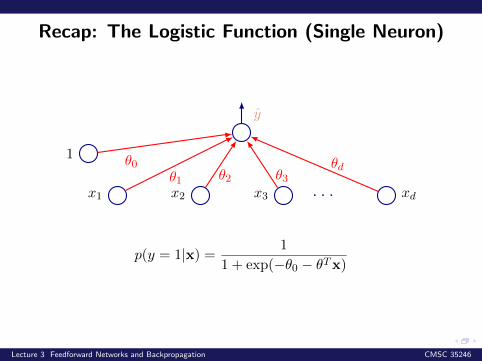
Recap: The Logistic Function (Single Neuron)
x1
1
x2 x3 . . . xd
y
θ1 θ2 θ3θdθ0
p(y = 1|x) = 1
1 + exp(−θ0 − θTx)
Lecture 3 Feedforward Networks and Backpropagation CMSC 35246
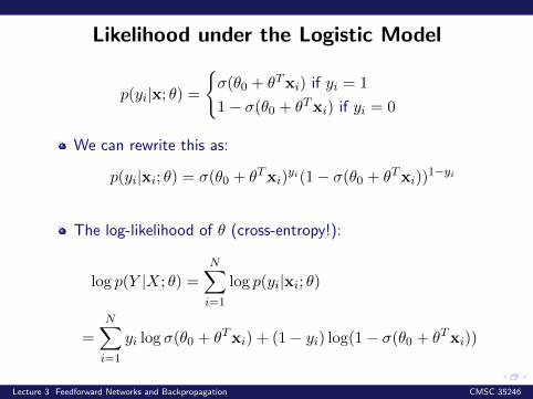
Likelihood under the Logistic Model
p(yi|x; θ) =
{σ(θ0 + θTxi) if yi = 1
1− σ(θ0 + θTxi) if yi = 0
We can rewrite this as:
p(yi|xi; θ) = σ(θ0 + θTxi)yi(1− σ(θ0 + θTxi))
1−yi
The log-likelihood of θ (cross-entropy!):
log p(Y |X; θ) =
N∑i=1
log p(yi|xi; θ)
=
N∑i=1
yi log σ(θ0 + θTxi) + (1− yi) log(1− σ(θ0 + θTxi))
Lecture 3 Feedforward Networks and Backpropagation CMSC 35246
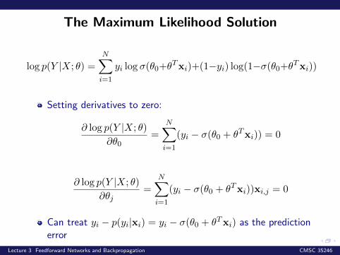
The Maximum Likelihood Solution
log p(Y |X; θ) =
N∑i=1
yi log σ(θ0+θTxi)+(1−yi) log(1−σ(θ0+θTxi))
Setting derivatives to zero:
∂ log p(Y |X; θ)
∂θ0=
N∑i=1
(yi − σ(θ0 + θTxi)) = 0
∂ log p(Y |X; θ)
∂θj=
N∑i=1
(yi − σ(θ0 + θTxi))xi,j = 0
Can treat yi − p(yi|xi) = yi − σ(θ0 + θTxi) as the predictionerror
Lecture 3 Feedforward Networks and Backpropagation CMSC 35246
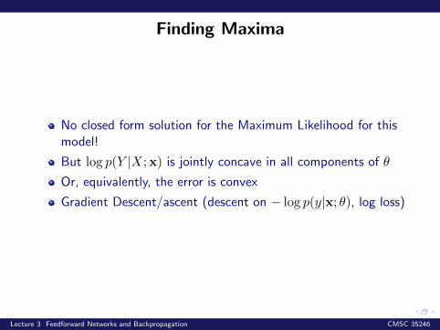
Finding Maxima
No closed form solution for the Maximum Likelihood for thismodel!
But log p(Y |X;x) is jointly concave in all components of θ
Or, equivalently, the error is convex
Gradient Descent/ascent (descent on − log p(y|x; θ), log loss)
Lecture 3 Feedforward Networks and Backpropagation CMSC 35246
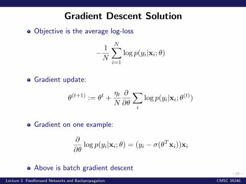
Gradient Descent Solution
Objective is the average log-loss
− 1
N
N∑i=1
log p(yi|xi; θ)
Gradient update:
θ(t+1) := θt +ηtN
∂
∂θ
∑i
log p(yi|xi; θ(t))
Gradient on one example:
∂
∂θlog p(yi|xi; θ) = (yi − σ(θTxi))xi
Above is batch gradient descent
Lecture 3 Feedforward Networks and Backpropagation CMSC 35246
Feedforward Networks
Lecture 3 Feedforward Networks and Backpropagation CMSC 35246
Introduction
Goal: Approximate some unknown ideal function f∗ : X → YIdeal classifier: y = f∗(x) with x and category y
Feedforward Network: Define parametric mappingy = f(x, θ)
Learn parameters θ to get a good approximation to f∗ fromavailable sample
Naming: Information flow in function evaluation begins atinput, flows through intermediate computations (that definethe function), to produce the category
No feedback connections (Recurrent Networks!)
Lecture 3 Feedforward Networks and Backpropagation CMSC 35246
Introduction
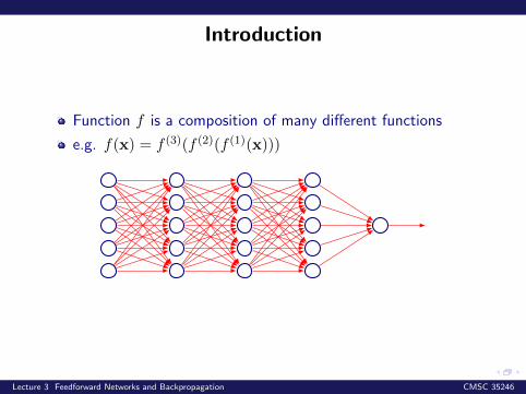
Function f is a composition of many different functions
e.g. f(x) = f (3)(f (2)(f (1)(x)))
Lecture 3 Feedforward Networks and Backpropagation CMSC 35246
Introduction
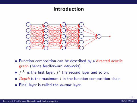
Function composition can be described by a directed acyclicgraph (hence feedforward networks)
f (1) is the first layer, f2 the second layer and so on.
Depth is the maximum i in the function composition chain
Final layer is called the output layer
Lecture 3 Feedforward Networks and Backpropagation CMSC 35246
Introduction
Training: Optimize θ to drive f(x; θ) closer to f∗(x)
Training Data: f∗ evaluated at different x instances (i.e.expected outputs)
Only specifies the output of the output layers
Output of intermediate layers is not specified by D, hence thenomenclature hidden layers
Neural: Choices of f (i)’s and layered organization, looselyinspired by neuroscience (first lecture)
Lecture 3 Feedforward Networks and Backpropagation CMSC 35246
Back to Linear Models
+ve: Optimization is convex or closed form!
-ve: Model can’t understand interaction between inputvariables!
Extension: Do nonlinear transformation x→ φ(x); applylinear model to φ(x)
φ gives features or a representation for x
How do we choose φ?
Lecture 3 Feedforward Networks and Backpropagation CMSC 35246
Choosing φ
Option 1: Use a generic φ
Example: Infinite dimensional φ implicitly used by kernelmachines with RBF kernel
Positive: Enough capacity to fit training data
Negative: Poor generalization for highly varying f∗
Prior used: Function is locally smooth.
Lecture 3 Feedforward Networks and Backpropagation CMSC 35246
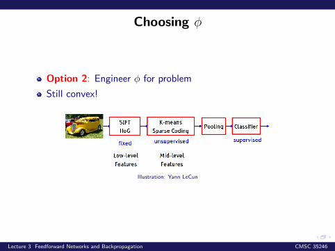
Choosing φ
Option 2: Engineer φ for problem
Still convex!
Illustration: Yann LeCun
Lecture 3 Feedforward Networks and Backpropagation CMSC 35246
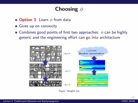
Choosing φ
Option 3: Learn φ from data
Gives up on convexity
Combines good points of first two approaches: φ can be highlygeneric and the engineering effort can go into architecture
Figure: Honglak Lee
Lecture 3 Feedforward Networks and Backpropagation CMSC 35246
Design Decisions
Need to choose optimizer, cost function and form of output
Choosing activation functions
Architecture design (number of layers etc)
Lecture 3 Feedforward Networks and Backpropagation CMSC 35246

Back to XOR
Lecture 3 Feedforward Networks and Backpropagation CMSC 35246
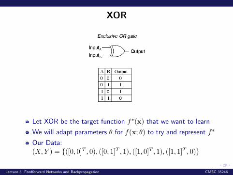
XOR
Let XOR be the target function f∗(x) that we want to learn
We will adapt parameters θ for f(x; θ) to try and represent f∗
Our Data:(X,Y ) = {([0, 0]T , 0), ([0, 1]T , 1), ([1, 0]T , 1), ([1, 1]T , 0)}
Lecture 3 Feedforward Networks and Backpropagation CMSC 35246
XOR
Our Data:(X,Y ) = {([0, 0]T , 0), ([0, 1]T , 1), ([1, 0]T , 1), ([1, 1]T , 0)}Not concerned with generalization, only want to fit this data
For simplicity consider the squared loss function
J(θ) =1
4
∑x∈X
(f∗(x)− f(x; θ))2
Need to choose a form for f(x; θ): Consider a linear modelwith θ being w and b
Our model f(x;w, b) = xTw + b
Lecture 3 Feedforward Networks and Backpropagation CMSC 35246
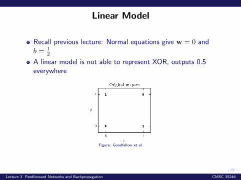
Linear Model
Recall previous lecture: Normal equations give w = 0 andb = 1
2
A linear model is not able to represent XOR, outputs 0.5everywhere
Figure: Goodfellow et al.
Lecture 3 Feedforward Networks and Backpropagation CMSC 35246
Solving XOR
How can we solve the XOR problem?
Idea: Learn a different feature space in which a linear modelwill work
Lecture 3 Feedforward Networks and Backpropagation CMSC 35246
Solving XOR
x1 x2
h1 h2
y
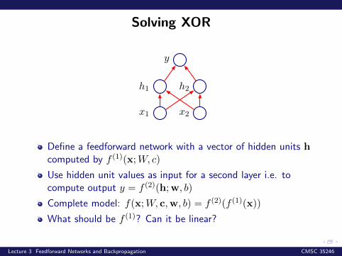
Define a feedforward network with a vector of hidden units hcomputed by f (1)(x;W, c)
Use hidden unit values as input for a second layer i.e. tocompute output y = f (2)(h;w, b)
Complete model: f(x;W, c,w, b) = f (2)(f (1)(x))
What should be f (1)? Can it be linear?
Lecture 3 Feedforward Networks and Backpropagation CMSC 35246
Solving XOR
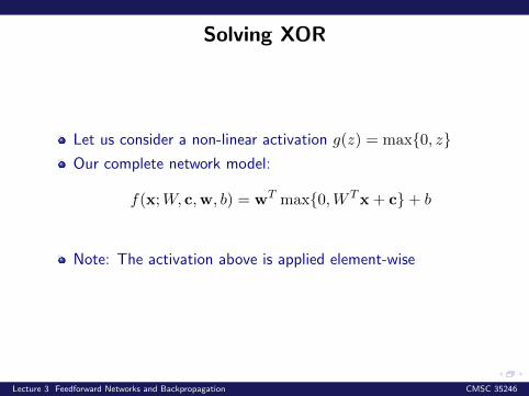
Let us consider a non-linear activation g(z) = max{0, z}Our complete network model:
f(x;W, c,w, b) = wT max{0,W Tx+ c}+ b
Note: The activation above is applied element-wise
Lecture 3 Feedforward Networks and Backpropagation CMSC 35246
A Solution
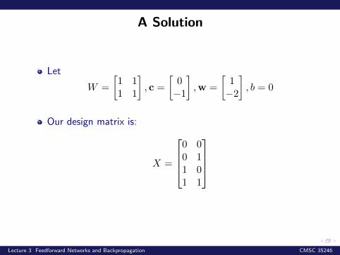
Let
W =
[1 11 1
], c =
[0−1
],w =
[1−2
], b = 0
Our design matrix is:
X =
0 00 11 01 1
Lecture 3 Feedforward Networks and Backpropagation CMSC 35246
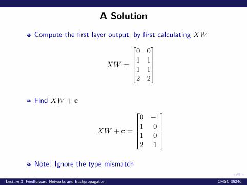
A Solution
Compute the first layer output, by first calculating XW
XW =
0 01 11 12 2
Find XW + c
XW + c =
0 −11 01 02 1
Note: Ignore the type mismatch
Lecture 3 Feedforward Networks and Backpropagation CMSC 35246
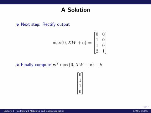
A Solution
Next step: Rectify output
max{0, XW + c} =
0 01 01 02 1
Finally compute wT max{0, XW + c}+ b
0110
Lecture 3 Feedforward Networks and Backpropagation CMSC 35246
Able to correctly classify every example in the set
This is a hand coded; demonstrative example, hence clean
For more complicated functions, we will proceed by usinggradient based learning
Lecture 3 Feedforward Networks and Backpropagation CMSC 35246
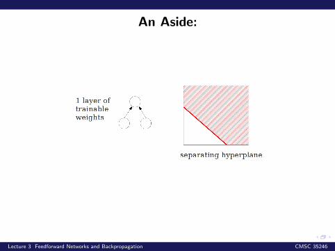
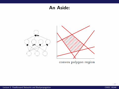
An Aside:
Lecture 3 Feedforward Networks and Backpropagation CMSC 35246
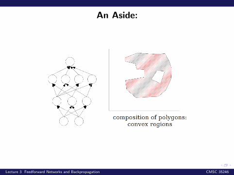
An Aside:
Lecture 3 Feedforward Networks and Backpropagation CMSC 35246
An Aside:
Lecture 3 Feedforward Networks and Backpropagation CMSC 35246
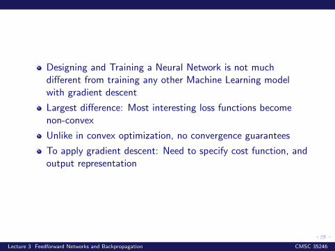
Designing and Training a Neural Network is not muchdifferent from training any other Machine Learning modelwith gradient descent
Largest difference: Most interesting loss functions becomenon-convex
Unlike in convex optimization, no convergence guarantees
To apply gradient descent: Need to specify cost function, andoutput representation
Lecture 3 Feedforward Networks and Backpropagation CMSC 35246
Cost Functions
Lecture 3 Feedforward Networks and Backpropagation CMSC 35246
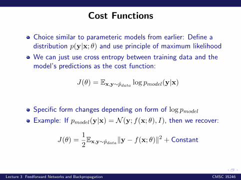
Cost Functions
Choice similar to parameteric models from earlier: Define adistribution p(y|x; θ) and use principle of maximum likelihood
We can just use cross entropy between training data and themodel’s predictions as the cost function:
J(θ) = Ex,y∼pdata log pmodel(y|x)
Specific form changes depending on form of log pmodel
Example: If pmodel(y|x) = N (y; f(x; θ), I), then we recover:
J(θ) =1
2Ex,y∼pdata‖y − f(x; θ)‖
2 + Constant
Lecture 3 Feedforward Networks and Backpropagation CMSC 35246
Cost Functions
Advantage: Need to specify p(y|x), and automatically get acost function log p(y|x)Choice of output units is very important for choice of costfunction
Lecture 3 Feedforward Networks and Backpropagation CMSC 35246

Output Units
Lecture 3 Feedforward Networks and Backpropagation CMSC 35246
Linear Units
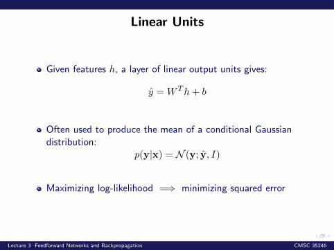
Given features h, a layer of linear output units gives:
y =W Th+ b
Often used to produce the mean of a conditional Gaussiandistribution:
p(y|x) = N (y; y, I)
Maximizing log-likelihood =⇒ minimizing squared error
Lecture 3 Feedforward Networks and Backpropagation CMSC 35246
Sigmoid Units
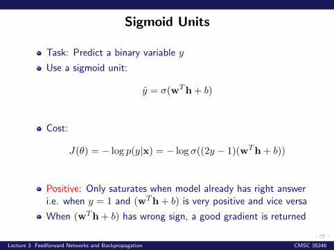
Task: Predict a binary variable y
Use a sigmoid unit:
y = σ(wTh+ b)
Cost:
J(θ) = − log p(y|x) = − log σ((2y − 1)(wTh+ b))
Positive: Only saturates when model already has right answeri.e. when y = 1 and (wTh+ b) is very positive and vice versa
When (wTh+ b) has wrong sign, a good gradient is returned
Lecture 3 Feedforward Networks and Backpropagation CMSC 35246
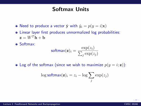
Softmax Units
Need to produce a vector y with yi = p(y = i|x)Linear layer first produces unnormalized log probabilities:z =W Th+ b
Softmax:
softmax(z)i =exp(zi)∑j exp(zj)
Log of the softmax (since we wish to maximize p(y = i; z)):
log softmax(z)i = zi − log∑j
exp(zj)
Lecture 3 Feedforward Networks and Backpropagation CMSC 35246
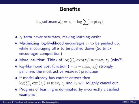
Benefits
log softmax(z)i = zi − log∑j
exp(zj)
zi term never saturates, making learning easier
Maximizing log-likelihood encourages zi to be pushed up,while encouraging all z to be pushed down (Softmaxencourages competition)
More intuition: Think of log∑
j exp(zj) ≈ maxj zj (why?)
log-likelihood cost function (∼ zi −maxj zj) stronglypenalizes the most active incorrect prediction
If model already has correct answer thenlog∑
j exp(zj) ≈ maxj zj and zi will roughly cancel out
Progress of learning is dominated by incorrectly classifiedexamples
Lecture 3 Feedforward Networks and Backpropagation CMSC 35246

Hidden Units
Lecture 3 Feedforward Networks and Backpropagation CMSC 35246
Hidden Units
Accept input x → compute affine transformationz =W Tx+ b → apply elementwise non-linear function g(z)→ obtain output g(z)
Choices for g?
Design of Hidden units is an active area of research
Lecture 3 Feedforward Networks and Backpropagation CMSC 35246
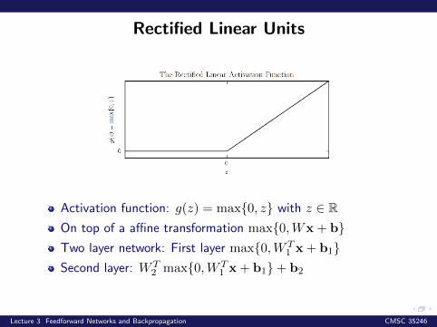
Rectified Linear Units
Activation function: g(z) = max{0, z} with z ∈ ROn top of a affine transformation max{0,Wx+ b}Two layer network: First layer max{0,W T
1 x+ b1}Second layer: W T
2 max{0,W T1 x+ b1}+ b2
Lecture 3 Feedforward Networks and Backpropagation CMSC 35246
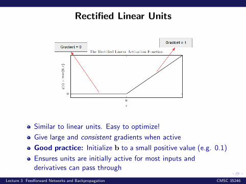
Rectified Linear Units
Similar to linear units. Easy to optimize!
Give large and consistent gradients when active
Good practice: Initialize b to a small positive value (e.g. 0.1)
Ensures units are initially active for most inputs andderivatives can pass through
Lecture 3 Feedforward Networks and Backpropagation CMSC 35246
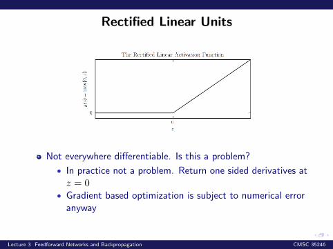
Rectified Linear Units
Not everywhere differentiable. Is this a problem?
• In practice not a problem. Return one sided derivatives atz = 0
• Gradient based optimization is subject to numerical erroranyway
Lecture 3 Feedforward Networks and Backpropagation CMSC 35246
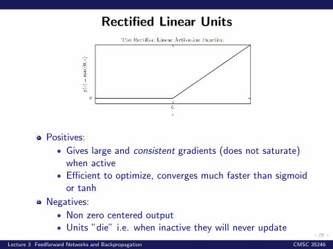
Rectified Linear Units
Positives:
• Gives large and consistent gradients (does not saturate)when active
• Efficient to optimize, converges much faster than sigmoidor tanh
Negatives:
• Non zero centered output• Units ”die” i.e. when inactive they will never update
Lecture 3 Feedforward Networks and Backpropagation CMSC 35246
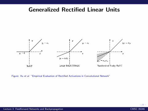
Generalized Rectified Linear Units
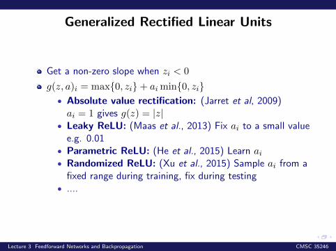
Get a non-zero slope when zi < 0
g(z, a)i = max{0, zi}+ aimin{0, zi}• Absolute value rectification: (Jarret et al, 2009)ai = 1 gives g(z) = |z|
• Leaky ReLU: (Maas et al., 2013) Fix ai to a small valuee.g. 0.01
• Parametric ReLU: (He et al., 2015) Learn ai• Randomized ReLU: (Xu et al., 2015) Sample ai from a
fixed range during training, fix during testing• ....
Lecture 3 Feedforward Networks and Backpropagation CMSC 35246
Generalized Rectified Linear Units
Figure: Xu et al. ”Empirical Evaluation of Rectified Activations in Convolutional Network”
Lecture 3 Feedforward Networks and Backpropagation CMSC 35246
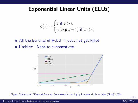
Exponential Linear Units (ELUs)
g(z) =
{z if z > 0
α(exp z − 1) if z ≤ 0
All the benefits of ReLU + does not get killed
Problem: Need to exponentiate
Figure: Clevert et al. ”Fast and Accurate Deep Network Learning by Exponential Linear Units (ELUs)”, 2016
Lecture 3 Feedforward Networks and Backpropagation CMSC 35246
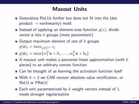
Maxout Units
Generalizes ReLUs further but does not fit into the (dotproduct → nonlinearity) mold
Instead of applying an element-wise function g(z), dividevector z into k groups (more parameters!)
Output maximum element of one of k groupsg(z)i = maxj∈G(i) zj
g(z)i = max{wT1 x+ b1, . . . , wTk x+ bk}
A maxout unit makes a piecewise linear approximation (with kpieces) to an arbitrary convex function
Can be thought of as learning the activation function itself
With k = 2 we CAN recover absolute value rectification, orReLU or PReLU
Each unit parameterized by k weight vectors instead of 1,needs stronger regularization
Lecture 3 Feedforward Networks and Backpropagation CMSC 35246
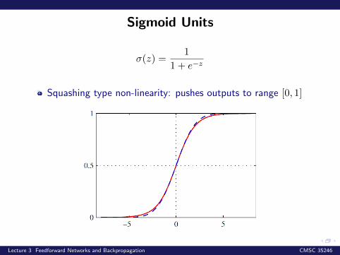
Sigmoid Units
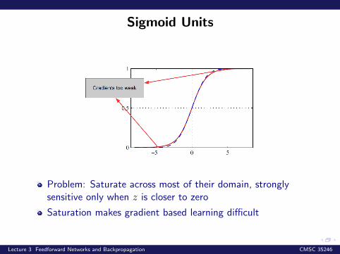
σ(z) =1
1 + e−z
Squashing type non-linearity: pushes outputs to range [0, 1]
Lecture 3 Feedforward Networks and Backpropagation CMSC 35246
Sigmoid Units
Problem: Saturate across most of their domain, stronglysensitive only when z is closer to zero
Saturation makes gradient based learning difficult
Lecture 3 Feedforward Networks and Backpropagation CMSC 35246
Tanh Units
Related to sigmoid: g(z) = tanh(z) = 2σ(2z)− 1
Positives: Squashes output to range [−1, 1], outputs arezero-centered
Negative: Also saturates
Still better than sigmoid as y = wT tanh(UT tanh(V Tx))resembles y = wTUTV Tx when activations are small
Lecture 3 Feedforward Networks and Backpropagation CMSC 35246
Other Units
Radial Basis Functions: g(z)i = exp(
1σ2i‖W:,ix‖2
)Function is more active as x approaches a template W:,i. Alsosaturates and is hard to train
Softplus: g(z) = log(1 + ez). Smooth version of rectifier(Dugas et al., 2001), although differentiable everywhere,empirically performs worse than rectifiers
Hard Tanh: g(z) = max(−1,min(1, z)), like the rectifier, butbounded (Collobert, 2004)
Lecture 3 Feedforward Networks and Backpropagation CMSC 35246
Summary
In Feedforward Networks don’t use Sigmoid
When a sigmoidal function must be used, use tanh
Use ReLU by default, but be careful with learning rates
Try other generalized ReLUs and Maxout for possibleimprovement
Lecture 3 Feedforward Networks and Backpropagation CMSC 35246

Universality and Depth
Lecture 3 Feedforward Networks and Backpropagation CMSC 35246
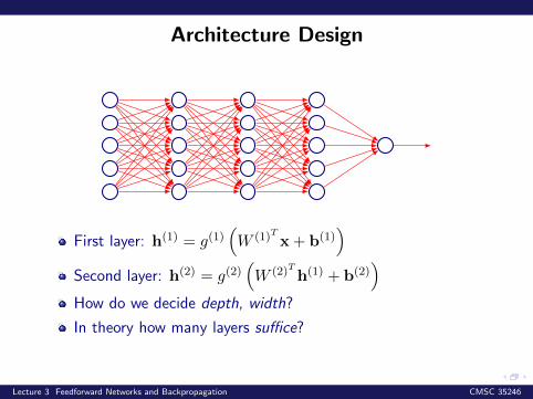
Architecture Design
First layer: h(1) = g(1)(W (1)Tx+ b(1)
)Second layer: h(2) = g(2)
(W (2)Th(1) + b(2)
)How do we decide depth, width?
In theory how many layers suffice?
Lecture 3 Feedforward Networks and Backpropagation CMSC 35246
Universality
Theoretical result [Cybenko, 1989]: 2-layer net with linearoutput with some squashing non-linearity in hidden units canapproximate any continuous function over compact domain toarbitrary accuracy (given enough hidden units!)
Implication: Regardless of function we are trying to learn, weknow a large MLP can represent this function
But not guaranteed that our training algorithm will be able tolearn that function
Gives no guidance on how large the network will be(exponential size in worst case)
Talked of some suggestive results earlier:
Lecture 3 Feedforward Networks and Backpropagation CMSC 35246
One more result:
(Montufar et al., 2014) Number of linear regions carved outby a deep rectifier network with d inputs, depth l and n unitsper hidden layer is:
O
((nd
)d(l−1)nd
)
Exponential in depth!
They showed functions representable with a deep rectifiernetwork can require an exponential number of hidden unitswith a shallow network
Lecture 3 Feedforward Networks and Backpropagation CMSC 35246
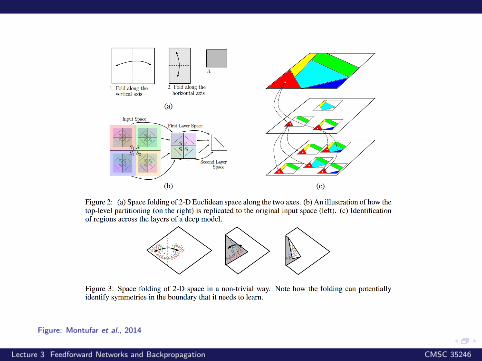
Figure: Montufar et al., 2014
Lecture 3 Feedforward Networks and Backpropagation CMSC 35246
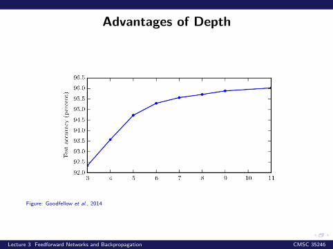
Advantages of Depth
Figure: Goodfellow et al., 2014
Lecture 3 Feedforward Networks and Backpropagation CMSC 35246
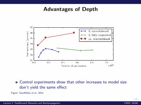
Advantages of Depth
Control experiments show that other increases to model sizedon’t yield the same effect
Figure: Goodfellow et al., 2014
Lecture 3 Feedforward Networks and Backpropagation CMSC 35246
Backpropagation: Introduction
Lecture 3 Feedforward Networks and Backpropagation CMSC 35246
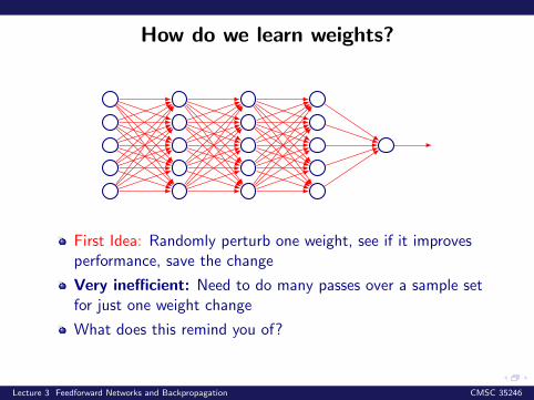
How do we learn weights?
First Idea: Randomly perturb one weight, see if it improvesperformance, save the change
Very inefficient: Need to do many passes over a sample setfor just one weight change
What does this remind you of?
Lecture 3 Feedforward Networks and Backpropagation CMSC 35246
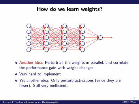
How do we learn weights?
Another Idea: Perturb all the weights in parallel, and correlatethe performance gain with weight changes
Very hard to implement
Yet another idea: Only perturb activations (since they arefewer). Still very inefficient.
Lecture 3 Feedforward Networks and Backpropagation CMSC 35246
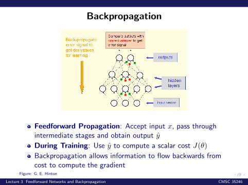
Backpropagation
Feedforward Propagation: Accept input x, pass throughintermediate stages and obtain output y
During Training: Use y to compute a scalar cost J(θ)
Backpropagation allows information to flow backwards fromcost to compute the gradient
Figure: G. E. Hinton
Lecture 3 Feedforward Networks and Backpropagation CMSC 35246
Backpropagation
From the training data we don’t know what the hidden unitsshould do
But, we can compute how fast the error changes as we changea hidden activity
Use error derivatives w.r.t hidden activities
Each hidden unit can affect many output units and haveseparate effects on error – combine these effects
Can compute error derivatives for hidden units efficiently (andonce we have error derivatives for hidden activities, easy toget error derivatives for weights going in)
Slide: G. E. Hinton
Lecture 3 Feedforward Networks and Backpropagation CMSC 35246
Review: neural networks
x1 x2
. . .xd
h h . . . h
f
w(1)11 w
(1)21 w
(1)d1
w(2)1 w
(2)2
w(2)m
h0 ≡ 1w
(2)0
x0 ≡ 1 w(1)01
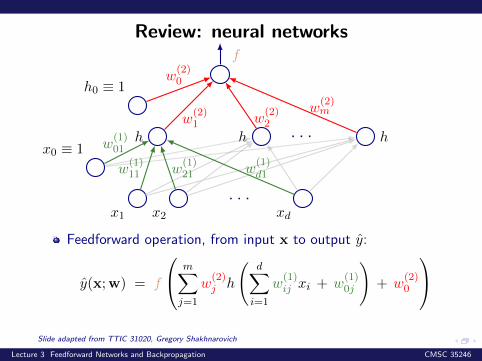
Feedforward operation, from input x to output y:
y(x;w) = f
m∑j=1
w(2)j h
(d∑i=1
w(1)ij xi + w
(1)0j
)+ w
(2)0
Slide adapted from TTIC 31020, Gregory Shakhnarovich
Lecture 3 Feedforward Networks and Backpropagation CMSC 35246
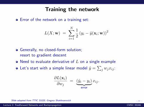
Training the network
Error of the network on a training set:
L(X;w) =
N∑i=1
1
2(yi − y(xi;w))2
Generally, no closed-form solution;resort to gradient descent
Need to evaluate derivative of L on a single example
Let’s start with a simple linear model y =∑
j wjxij :
∂L(xi)
∂wj= (yi − yi)︸ ︷︷ ︸
error
xij .
Slide adapted from TTIC 31020, Gregory Shakhnarovich
Lecture 3 Feedforward Networks and Backpropagation CMSC 35246
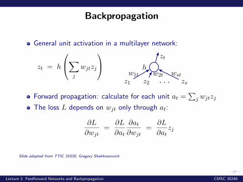
Backpropagation
General unit activation in a multilayer network:
zt = h
∑j
wjtzj
h
z1
w1t
z2w2t. . . zs
wst
zt
Forward propagation: calculate for each unit at =∑
j wjtzj
The loss L depends on wjt only through at:
∂L
∂wjt=
∂L
∂at
∂at∂wjt
=∂L
∂atzj
Slide adapted from TTIC 31020, Gregory Shakhnarovich
Lecture 3 Feedforward Networks and Backpropagation CMSC 35246
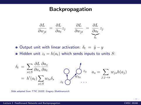
Backpropagation
∂L
∂wjt=
∂L
∂atzj
∂L
∂wjt=
∂L
∂at︸︷︷︸δt
zj
Output unit with linear activation: δt = y − yHidden unit zt = h(at) which sends inputs to units S:
δt =∑s∈S
∂L
∂as
∂as∂at
= h′(at)∑s∈S
wtsδszt . . .
zswts
as =∑j:j→s
wjsh(aj)
Slide adapted from TTIC 31020, Gregory Shakhnarovich
Lecture 3 Feedforward Networks and Backpropagation CMSC 35246
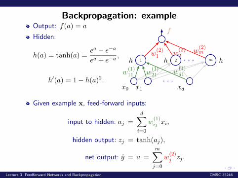
Backpropagation: exampleOutput: f(a) = a
Hidden:
h(a) = tanh(a) =ea − e−a
ea + e−a,
h′(a) = 1− h(a)2.x0 x1
. . .xd
1h 2h . . . m h
f
w(1)11 w
(1)21
w(1)d1
w(2)1 w
(2)2
w(2)m
Given example x, feed-forward inputs:
input to hidden: aj =d∑i=0
w(1)ij xi,
hidden output: zj = tanh(aj),
net output: y = a =
m∑j=0
w(2)j zj .
Lecture 3 Feedforward Networks and Backpropagation CMSC 35246
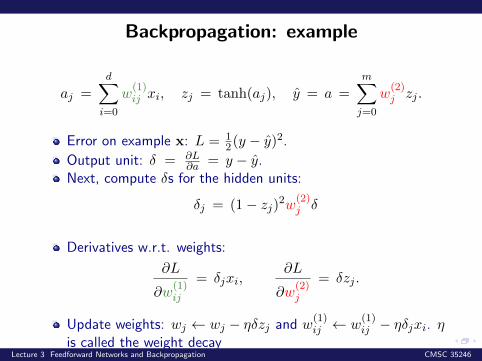
Backpropagation: example
aj =
d∑i=0
w(1)ij xi, zj = tanh(aj), y = a =
m∑j=0
w(2)j zj .
Error on example x: L = 12(y − y)
2.
Output unit: δ = ∂L∂a = y − y.
Next, compute δs for the hidden units:
δj = (1− zj)2w(2)j δ
Derivatives w.r.t. weights:
∂L
∂w(1)ij
= δjxi,∂L
∂w(2)j
= δzj .
Update weights: wj ← wj − ηδzj and w(1)ij ← w
(1)ij − ηδjxi. η
is called the weight decayLecture 3 Feedforward Networks and Backpropagation CMSC 35246
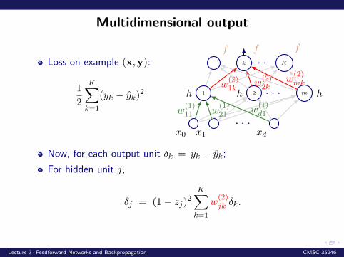
Multidimensional output
Loss on example (x,y):
1
2
K∑k=1
(yk − yk)2
x0 x1. . .
xd
1h 2h . . . m h
fk
f. . . K
f
w(1)11 w
(1)21
w(1)d1
w(2)1k
w(2)2k
w(2)mk
Now, for each output unit δk = yk − yk;
For hidden unit j,
δj = (1− zj)2K∑k=1
w(2)jk δk.
Lecture 3 Feedforward Networks and Backpropagation CMSC 35246
Next time
More Backpropagation
Start with Regularization in Neural Networks
Quiz
Lecture 3 Feedforward Networks and Backpropagation CMSC 35246