lecture 13 newton-raphson power flow professor tom overbye department of electrical and computer...
TRANSCRIPT

Lecture 13Newton-Raphson Power Flow
Professor Tom OverbyeDepartment of Electrical and
Computer Engineering
ECE 476
POWER SYSTEM ANALYSIS

2
Announcements
Homework 6 is due on Thursday (Oct 18) Be reading Chapter 6 Homework 7 is 6.12, 6.19, 6.22, 6.45 and 6.50.
Due date is October 25

3
Design Project
Design Project 2 from the book is assigned today (page 345 to 348). It will be due Nov 29. For a transmission tower configuration assume a symmetrical tower configuration with individual conductor spacings as provided on the handout sheet.

4
Newton-Raphson Algorithm
The second major power flow solution method is the Newton-Raphson algorithm
Key idea behind Newton-Raphson is to use sequential linearization
General form of problem: Find an x such that
( ) 0ˆf x

5
Newton-Raphson Method (scalar)
( )
( ) ( )
( )( ) ( )
2 ( ) 2( )2
1. For each guess of , , define ˆ
-ˆ
2. Represent ( ) by a Taylor series about ( )ˆ
( )( ) ( )ˆ
1 ( )higher order terms
2
v
v v
vv v
vv
x x
x x x
f x f x
df xf x f x x
dx
d f xx
dx

6
Newton-Raphson Method, cont’d
( )( ) ( )
( )
1( )( ) ( )
3. Approximate ( ) by neglecting all terms ˆ
except the first two
( )( ) 0 ( )ˆ
4. Use this linear approximation to solve for
( )( )
5. Solve for a new estim
vv v
v
vv v
f x
df xf x f x x
dx
x
df xx f x
dx
( 1) ( ) ( )
ate of x̂v v vx x x
7
Newton-Raphson Example
2
1( )( ) ( )
( ) ( ) 2( )
( 1) ( ) ( )
( 1) ( ) ( ) 2( )
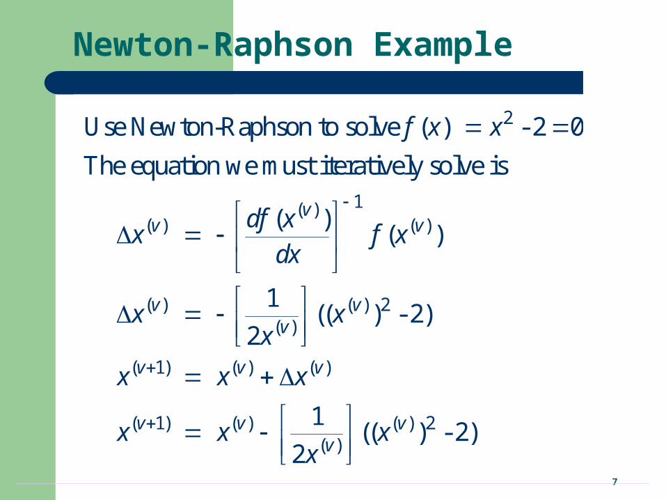
Use Newton-Raphson to solve ( ) - 2 0
The equation we must iteratively solve is
( )( )
1(( ) - 2)
2
1(( ) - 2)
2
vv v
v vv
v v v
v v vv
f x x
df xx f x
dx
x xx
x x x
x x xx
8
Newton-Raphson Example, cont’d
( 1) ( ) ( ) 2( )
(0)
( ) ( ) ( )
3 3
6
1(( ) - 2)
2
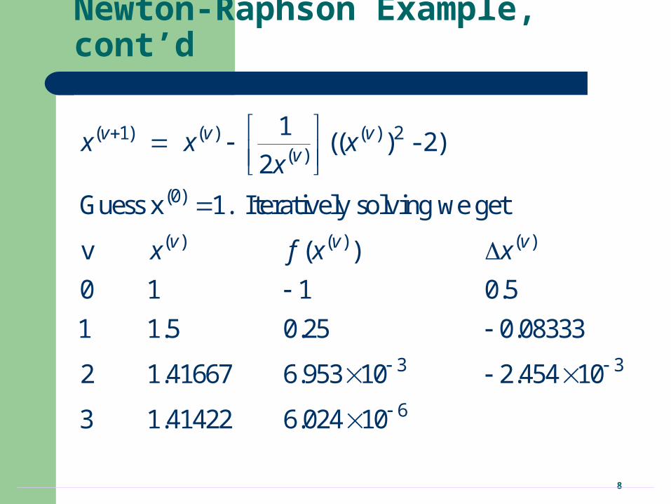
Guess x 1. Iteratively solving we get
v ( )
0 1 1 0.5
1 1.5 0.25 0.08333
2 1.41667 6.953 10 2.454 10
3 1.41422 6.024 10
v v vv
v v v
x x xx
x f x x

9
Newton-Raphson Comments
When close to the solution the error decreases quite quickly -- method has quadratic convergence
f(x(v)) is known as the mismatch, which we would like to drive to zero
Stopping criteria is when f(x(v)) < Results are dependent upon the initial guess. What if we had
guessed x(0) = 0, or x (0) = -1? A solution’s region of attraction (ROA) is the set of initial
guesses that converge to the particular solution. The ROA is often hard to determine

10
Multi-Variable Newton-Raphson
1 1
2 2
Next we generalize to the case where is an n-
dimension vector, and ( ) is an n-dimension function
( )
( )( )
( )
Again define the solution so ( ) 0 andˆ ˆn n
x f
x f
x f
x
f x
x
xx f x
x
x f x
x
ˆ x x

11
Multi-Variable Case, cont’d
i
1 11 1 1 2
1 2
1
n nn n 1 2
1 2
n
The Taylor series expansion is written for each f ( )
f ( ) f ( )f ( ) f ( )ˆ
f ( )higher order terms
f ( ) f ( )f ( ) f ( )ˆ
f ( )higher order terms
nn
nn
x xx x
xx
x xx x
xx
x
x xx x
x
x xx x
x

12
Multi-Variable Case, cont’d
1 1 1
1 21 1
2 2 22 2
1 2
1 2
This can be written more compactly in matrix form
( ) ( ) ( )
( )( ) ( ) ( )
( )( )ˆ
( )( ) ( ) ( )
n
n
nn n n
n
f f fx x x
f xf f f
f xx x x
ff f fx x x
x x x
xx x x
xf x
xx x x
higher order terms
nx
13
Jacobian Matrix
1 1 1
1 2
2 2 2
1 2
1 2
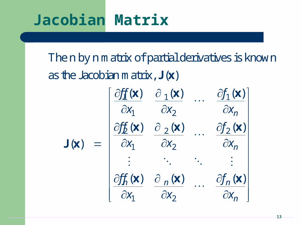
The n by n matrix of partial derivatives is known
as the Jacobian matrix, ( )
( ) ( ) ( )
( ) ( ) ( )
( )
( ) ( ) ( )
n
n
n n n
n
f f fx x x
f f fx x x
f f fx x x
J x
x x x
x x x
J x
x x x

14
Multi-Variable N-R Procedure
1
( 1) ( ) ( )
( 1) ( ) ( ) 1 ( )
( )
Derivation of N-R method is similar to the scalar case
( ) ( ) ( ) higher order termsˆ
( ) 0 ( ) ( )ˆ
( ) ( )
( ) ( )
Iterate until ( )
v v v
v v v v
v
f x f x J x x
f x f x J x x
x J x f x
x x x
x x J x f x
f x

15
Multi-Variable Example
1
2
2 21 1 2
2 22 1 2 1 2
1 1
1 2
2 2
1 2
xSolve for = such that ( ) 0 where
x
f ( ) 2 8 0
f ( ) 4 0
First symbolically determine the Jacobian
f ( ) f ( )
( ) =f ( ) f ( )
x x
x x x x
x x
x x
x f x
x
x
x x
J xx x

16
Multi-variable Example, cont’d
1 2
1 2 1 2
11 1 2 1
2 1 2 1 2 2
(0)
1(1)
4 2( ) =
2 2
Then
4 2 ( )
2 2 ( )
1Arbitrarily guess
1
1 4 2 5 2.1
1 3 1 3 1.3
x x
x x x x
x x x f
x x x x x f
J x
x
x
x
x

17
Multi-variable Example, cont’d
1(2)
(2)
2.1 8.40 2.60 2.51 1.8284
1.3 5.50 0.50 1.45 1.2122
Each iteration we check ( ) to see if it is below our
specified tolerance
0.1556( )
0.0900
If = 0.2 then we wou
x
f x
f x
ld be done. Otherwise we'd
continue iterating.

18
NR Application to Power Flow
** * *
i1 1
We first need to rewrite complex power equations
as equations with real coefficients
S
These can be derived by defining
Recal
i
n n
i i i ik k i ik kk k
ik ik ik
ji i i i
ik i k
V I V Y V V Y V
Y G jB
V V e V
jl e cos sinj

19
Real Power Balance Equations
* *i
1 1
1
i1
i1
S ( )
(cos sin )( )
Resolving into the real and imaginary parts
P ( cos sin )
Q ( sin cos
ikn n
ji i i ik k i k ik ik
k k
n
i k ik ik ik ikk
n
i k ik ik ik ik Gi Dik
n
i k ik ik ik ik
P jQ V Y V V V e G jB
V V j G jB
V V G B P P
V V G B
)k Gi DiQ Q

20
Newton-Raphson Power Flow
i1
In the Newton-Raphson power flow we use Newton's
method to determine the voltage magnitude and angle
at each bus in the power system.
We need to solve the power balance equations
P ( cosn
i k ik ikk
V V G
i1
sin )
Q ( sin cos )
ik ik Gi Di
n
i k ik ik ik ik Gi Dik
B P P
V V G B Q Q

21
Power Flow Variables
2 2 2
n
2
Assume the slack bus is the first bus (with a fixed
voltage angle/magnitude). We then need to determine
the voltage angle/magnitude at the other buses.
( )
( )
G
n
P P
V
V
x
x f x
2
2 2 2
( )
( )
( )
D
n Gn Dn
G D
n Gn Dn
P
P P P
Q Q Q
Q Q Q
x
x
x

22
N-R Power Flow Solution
( )
( )
( 1) ( ) ( ) 1 ( )
The power flow is solved using the same procedure
discussed last time:
Set 0; make an initial guess of ,
While ( ) Do
( ) ( )
1
End While
v
v
v v v v
v
v v
x x
f x
x x J x f x

23
Power Flow Jacobian Matrix
1 1 1
1 2
2 2 2
1 2
1 2
The most difficult part of the algorithm is determining
and inverting the n by n Jacobian matrix, ( )
( ) ( ) ( )
( ) ( ) ( )
( )
( ) ( ) ( )
n
n
n n n
n
f f fx x x
f f fx x x
f f fx x x
J x
x x x
x x x
J x
x x x

24
Power Flow Jacobian Matrix, cont’d
i
i
i1
Jacobian elements are calculated by differentiating
each function, f ( ), with respect to each variable.
For example, if f ( ) is the bus i real power equation
f ( ) ( cos sin )n
i k ik ik ik ik Gik
x V V G B P P
x
x
i
1
i
f ( )( sin cos )
f ( )( sin cos ) ( )
Di
n
i k ik ik ik iki k
k i
i j ik ik ik ikj
xV V G B
xV V G B j i

25
Two Bus Newton-Raphson Example
Line Z = 0.1j
One Two 1.000 pu 1.000 pu
200 MW 100 MVR
0 MW 0 MVR
For the two bus power system shown below, use the Newton-Raphson power flow to determine the voltage magnitude and angle at bus two. Assumethat bus one is the slack and SBase = 100 MVA.
2
2
10 10
10 10busj j
V j j
x Y

26
Two Bus Example, cont’d
i1
i1
2 2 1 2
22 2 1 2 2
General power balance equations
P ( cos sin )
Q ( sin cos )
Bus two power balance equations
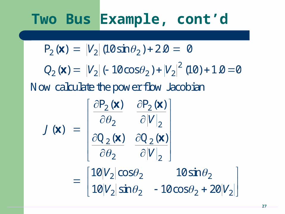
P (10sin ) 2.0 0
( 10cos ) (10) 1.0 0
n
i k ik ik ik ik Gi Dik
n
i k ik ik ik ik Gi Dik
V V G B P P
V V G B Q Q
V V
Q V V V
27
Two Bus Example, cont’d
2 2 2
22 2 2 2
2 2
2 2
2 2
2 2
2 2 2
2 2 2 2
P ( ) (10sin ) 2.0 0
( ) ( 10cos ) (10) 1.0 0
Now calculate the power flow Jacobian
P ( ) P ( )
( )Q ( ) Q ( )
10 cos 10sin
10 sin 10cos 20
V
Q V V
VJ
V
V
V V
x
x
x x
xx x

28
Two Bus Example, First Iteration
(0)
2 2(0)2
2 2 2
2 2 2(0)
2 2 2 2
(1)
0Set 0, guess
1
Calculate
(10sin ) 2.0 2.0f( )
1.0( 10cos ) (10) 1.0
10 cos 10sin 10 0( )
10 sin 10cos 20 0 10
0 10 0Solve
1 0 10
v
V
V V
V
V V
x
x
J x
x1 2.0 0.2
1.0 0.9

29
Two Bus Example, Next Iterations
(1)2
(1)
1(2)
0.9(10sin( 0.2)) 2.0 0.212f( )
0.2790.9( 10cos( 0.2)) 0.9 10 1.0
8.82 1.986( )
1.788 8.199
0.2 8.82 1.986 0.212 0.233
0.9 1.788 8.199 0.279 0.8586
f(
x
J x
x
(2) (3)
(3)2
0.0145 0.236)
0.0190 0.8554
0.0000906f( ) Done! V 0.8554 13.52
0.0001175
x x
x

30
Two Bus Solved Values
Line Z = 0.1j
One Two 1.000 pu 0.855 pu
200 MW 100 MVR
200.0 MW168.3 MVR
-13.522 Deg
200.0 MW 168.3 MVR
-200.0 MW-100.0 MVR
Once the voltage angle and magnitude at bus 2 are known we can calculate all the other system values,such as the line flows and the generator reactive power output

31
Two Bus Case Low Voltage Solution
(0)
2 2(0)2
2 2 2
This case actually has two solutions! The second
"low voltage" is found by using a low initial guess.
0Set 0, guess
0.25
Calculate
(10sin ) 2.0f( )
( 10cos ) (10) 1.0
v
V
V V
x
x
2 2 2(0)
2 2 2 2
2
0.875
10 cos 10sin 2.5 0( )
10 sin 10cos 20 0 5
V
V V
J x

32
Low Voltage Solution, cont'd
1(1)
(2) (2) (3)
0 2.5 0 2 0.8Solve
0.25 0 5 0.875 0.075
1.462 1.42 0.921( )
0.534 0.2336 0.220
x
f x x x
Line Z = 0.1j
One Two 1.000 pu 0.261 pu
200 MW 100 MVR
200.0 MW831.7 MVR
-49.914 Deg
200.0 MW 831.7 MVR
-200.0 MW-100.0 MVR
Low voltage solution

33
Two Bus Region of Convergence
Slide shows the region of convergence for different initialguesses of bus 2 angle (x-axis) and magnitude (y-axis)
Red regionconvergesto the highvoltage solution,while the yellow regionconvergesto the lowvoltage solution

34
PV Buses
Since the voltage magnitude at PV buses is fixed there is no need to explicitly include these voltages in x or write the reactive power balance equations– the reactive power output of the generator varies to
maintain the fixed terminal voltage (within limits)– optionally these variations/equations can be included by
just writing the explicit voltage constraint for the generator bus
|Vi | – Vi setpoint = 0

35
Three Bus PV Case Example
Line Z = 0.1j
Line Z = 0.1j Line Z = 0.1j
One Two 1.000 pu 0.941 pu
200 MW 100 MVR
170.0 MW 68.2 MVR
-7.469 Deg
Three 1.000 pu
30 MW 63 MVR
2 2 2 2
3 3 3 3
2 2 2
For this three bus case we have
( )
( ) ( ) 0
V ( )
G D
G D
D
P P P
P P P
Q Q
x
x f x x
x

36
Modeling Voltage Dependent Load
So far we've assumed that the load is independent of
the bus voltage (i.e., constant power). However, the
power flow can be easily extended to include voltage
depedence with both the real and reactive l
Di Di
1
1
oad. This
is done by making P and Q a function of :
( cos sin ) ( ) 0
( sin cos ) ( ) 0
i
n
i k ik ik ik ik Gi Di ik
n
i k ik ik ik ik Gi Di ik
V
V V G B P P V
V V G B Q Q V

37
Voltage Dependent Load Example
22 2 2 2
2 22 2 2 2 2
2 2 2 2
In previous two bus example now assume the load is
constant impedance, so
P ( ) (10sin ) 2.0 0
( ) ( 10cos ) (10) 1.0 0
Now calculate the power flow Jacobian
10 cos 10sin 4.0( )
10
V V
Q V V V
V VJ
x
x
x2 2 2 2 2sin 10cos 20 2.0V V V

38
Voltage Dependent Load, cont'd
(0)
22 2 2(0)
2 22 2 2 2
(0)
1(1)
0Again set 0, guess
1
Calculate
(10sin ) 2.0 2.0f( )
1.0( 10cos ) (10) 1.0
10 4( )
0 12
0 10 4 2.0 0.1667Solve
1 0 12 1.0 0.9167
v
V V
V V V
x
x
J x
x
39
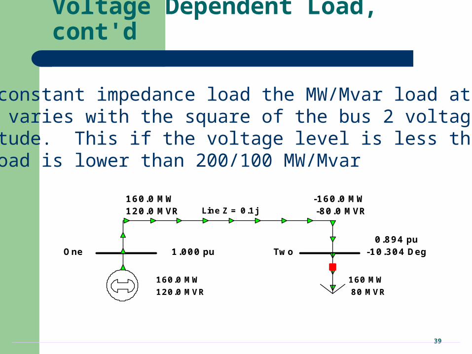
Voltage Dependent Load, cont'd
Line Z = 0.1j
One Two 1.000 pu 0.894 pu
160 MW 80 MVR
160.0 MW120.0 MVR
-10.304 Deg
160.0 MW 120.0 MVR
-160.0 MW -80.0 MVR
With constant impedance load the MW/Mvar load atbus 2 varies with the square of the bus 2 voltage magnitude. This if the voltage level is less than 1.0,the load is lower than 200/100 MW/Mvar

40
Solving Large Power Systems
The most difficult computational task is inverting the Jacobian matrix– inverting a full matrix is an order n3 operation, meaning
the amount of computation increases with the cube of the size size
– this amount of computation can be decreased substantially by recognizing that since the Ybus is a sparse matrix, the Jacobian is also a sparse matrix
– using sparse matrix methods results in a computational order of about n1.5.
– this is a substantial savings when solving systems with tens of thousands of buses

41
Newton-Raphson Power Flow
Advantages– fast convergence as long as initial guess is close to solution– large region of convergence
Disadvantages– each iteration takes much longer than a Gauss-Seidel iteration– more complicated to code, particularly when implementing
sparse matrix algorithms
Newton-Raphson algorithm is very common in power flow analysis