lecture #13 more machine learning - kth

15-‐05-‐16

1

KTH ROYAL INSTITUTE OF TECHNOLOGY

Lecture #13 More Machine Learning

On the Shoulder of Giants

Much of the material in this slide set is based upon: ”Automated Learning techniques in Power Systems” by L. Wehenkel, Université Liege ”Probability based learning” Josephine Sullivan, KTH ”Entropy and Information Gain” by F.Aiolli, University of Padova

15-‐05-‐16

2

Contents

Repeating from last time Artificial Neural Networks K-Nearest Neighbour

Power Systems Analysis – An automated learning approach

Understanding states in the power system is established through observation of inputs and outputs without regard to the physical electrotechnical relations between the states. Adding knowledge about the electrotechnical rules means adding heuristics to the learning.

Someinput

Someoutput

P(X)

15-‐05-‐16

3

Classes of methods for learning

In Supervised learning a set of input data and output data is provided, and with the help of these two datasets the model of the system is created. In Unsupervised learning, no ideal model is anticipated, but instead the analysis of the states is done in order to identify possible correlations bewteen datapoints. In Reinforced learning, the model in the system can be gradually refined through means of a utility function, that tells the system that a certain ouput is more suitable than another.

For this introductory course, our

focus is here With a short

look at unsupervised

learning

Classification vs Regression

Two forms of Supervised learning Classification: The input data is number of switch operations a circuitbreaker has performed and tthe output is a notification whether the switch needs maintenance or not. ”Boolean” Regression: Given the wind speed in a incoming weather front, the output is the anticipated production in a set of wind turbines. ”Floating point”

15-‐05-‐16

4

Supervised learning - a preview

In the scope of this course, we will be studying three forms of supervised learning.

•  Decision Trees Overview and practical work on exercise session.

•  Artificial Neural Networks Overview only, no practical work.

•  Statistical methods – k-Nearest Neighbour

Overview and practical work on exercise session. Also included in Project Assignment kNN algorithm can also be used for unsupervised clustering.

Example from Automatic Learning techniques in Power Systems

One Machine Infinite Bus (OMIB) system •  Assuming a fault close to the Generator will be cleared

within 155 ms by protection relays •  We need to identify situations in which this clearing time is

sufficient and when it is not •  Under certain loading situations, 155 ms may be too slow.

Source: Automatic Learning techniques in Power Systems, L. Wehenkel

15-‐05-‐16

5

OMIB – further information

In the OMIB system the following parameters influence security •  Amount of active and reactive power of the generator ( •  Amount of load nearby the generator (PI) •  Voltage magnitudes at the load bus and at the infinite bus

Short-circuit reactance Xinf, representing the effect of variable topology in the large system represented by the infinite bus.

In the example, Voltages at generator and Infinite bus are assumed similar and constant for simplicity


Our database of objects with attributes

In a simulator, we randomly sample values for Pu and Qu creating a database with 5000 samples (objects) and for each object we have a set of attributes (Pu, Qu, V1, P1, Vinf, Xinf, CCT) as per below.


15-‐05-‐16

6

Plot of database content


How to measure information content

Entropy H is a measure of Unpredictability. Defined as:

� Where

pi is the probability of event i

15-‐05-‐16

7

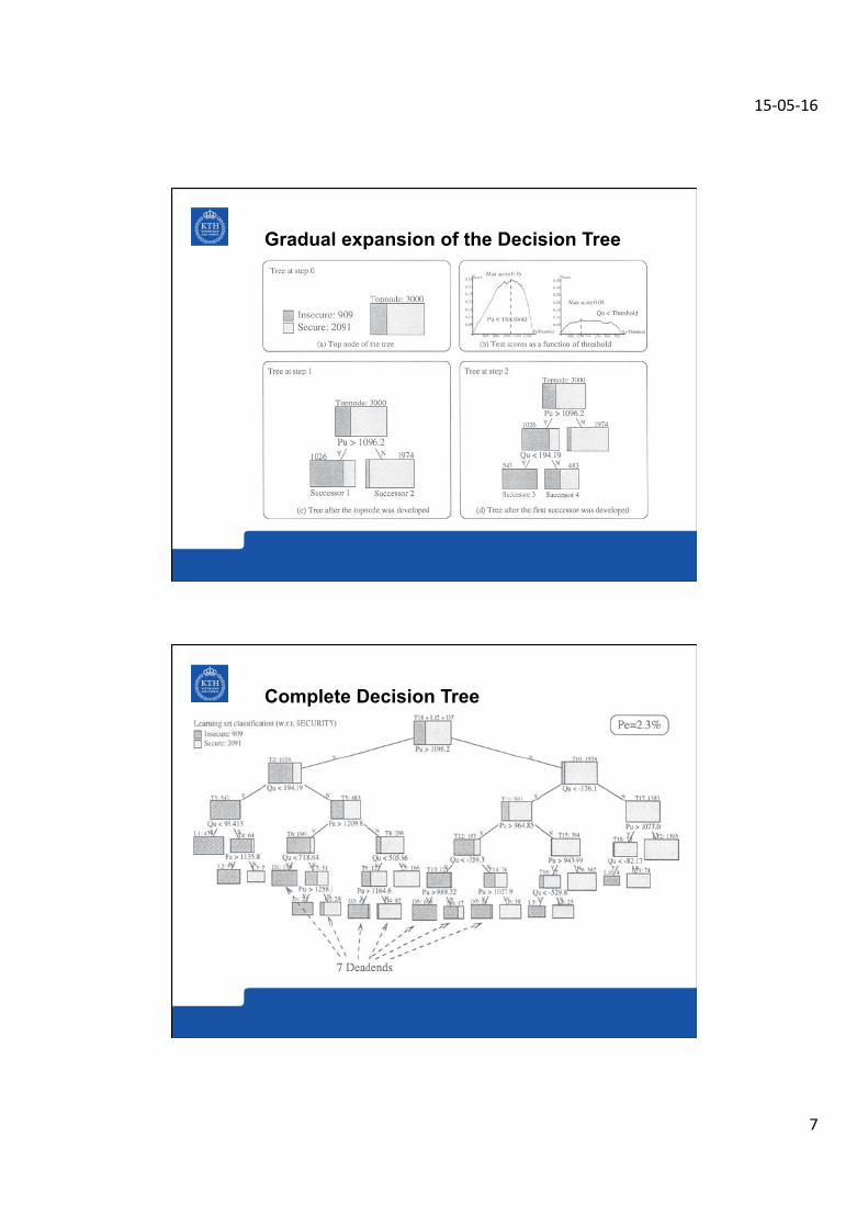
Gradual expansion of the Decision Tree

Complete Decision Tree

15-‐05-‐16

8

How to stop?

The splitting of data sets continues until either: A perfect partition is reached – i.e. One which perfecly explains the content of the class – a leaf One where no infomration is gained no matter how the data set is split. – a deadend.

Validation of the Decision Tree

By using the Test Set (2000 samples) we can calidate the Decision tree. By testing for each Object in the Test Set, we determine if the Decision tree provides the right answer for the Object. In this particular example, the probability o error can be determined to 2,3. I.e. Of the 2000 samples 46 were classififed to the wrong class.

15-‐05-‐16

9

Contents


Artificial Neural Networks - Introduction

Inspired by the Human Nerve system A close resemblance ?

15-‐05-‐16

10

The Perceptron – Artifical Neuron

•  The perceptron takes inputs x •  The inputs are weighted w •  The Perceptron sums the values of the inputs •  Provides as output a threshold function based on the sum •  Linear perceptron provides sum as output •  Non-linear provide a output function.

x

w

Non Linear Perceptrons

Linear Perceptrons provide output as sum of weighted inputs. Non-linear perceptrons normally use a threhold function for the output, to limit the extreme values. Some examples are: tanh(x) Signmoidal function 0 -> 0,5 << -1 -> 0 >>1 -> 1

15-‐05-‐16

11

Artificial Neural Network

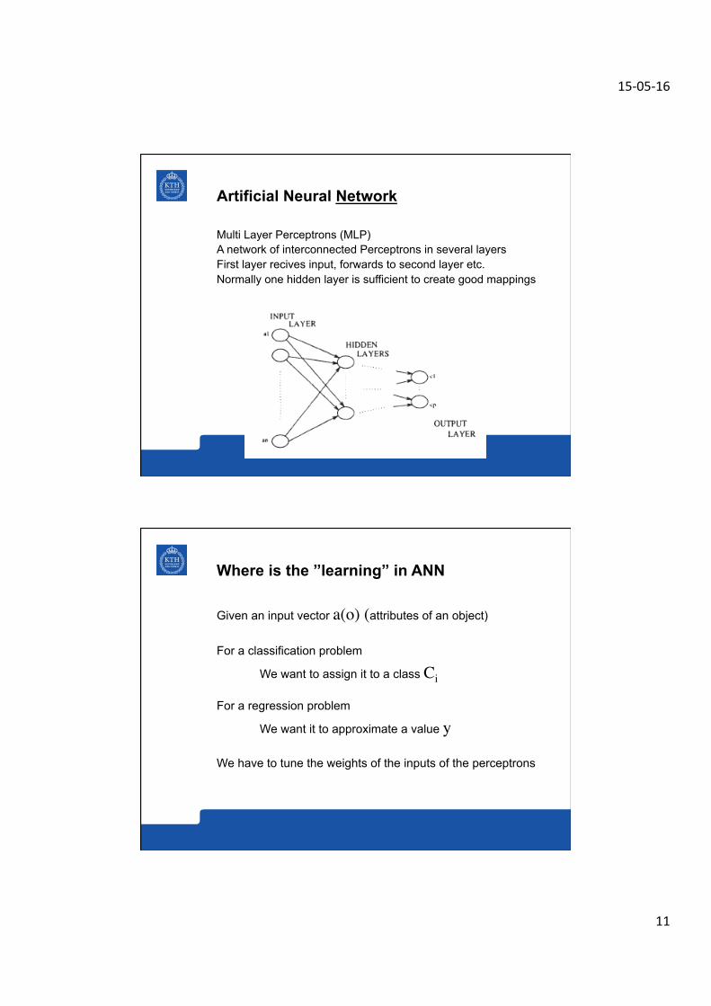
Multi Layer Perceptrons (MLP) A network of interconnected Perceptrons in several layers First layer recives input, forwards to second layer etc. Normally one hidden layer is sufficient to create good mappings

Where is the ”learning” in ANN

Given an input vector a(o) (attributes of an object) For a classification problem

We want to assign it to a class Ci

For a regression problem

We want it to approximate a value y

We have to tune the weights of the inputs of the perceptrons

15-‐05-‐16

12

So how to tune the weights in this …?

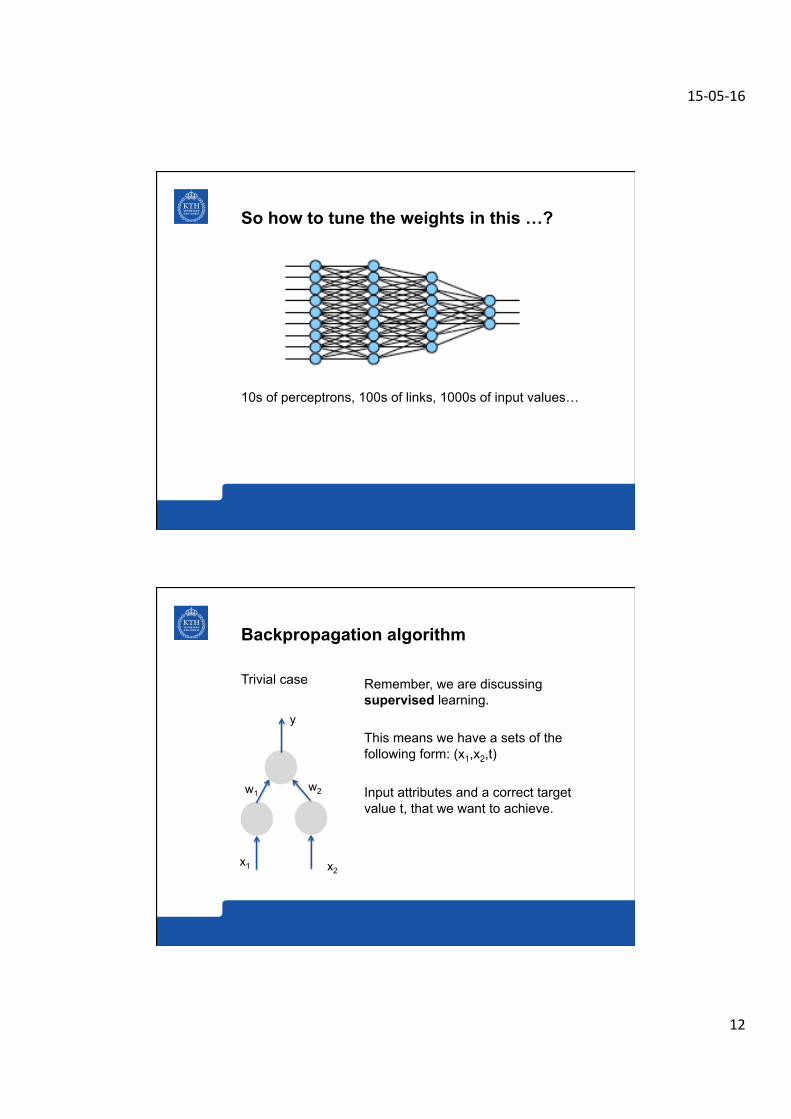
10s of perceptrons, 100s of links, 1000s of input values…

Backpropagation algorithm

Trivial case

x1 x2

w2 w1

y

Remember, we are discussing supervised learning. This means we have a sets of the following form: (x1,x2,t)

Input attributes and a correct target value t, that we want to achieve.

15-‐05-‐16

13

Backpropagation algorithm

Trivial case

x1 x2

w2 w1

y

The Least Squares Error

E = (t - y)2

For a linear Perceptron

y = x1w1 + x2w2Find minima of E(y) w.r.t (w1,w2)

Finding minima - gradient descent

In the general case, we want to find the minima of the Error function with regards to the weights If we can find the derivative of the error function, we can use that to find a suitable adjustment of the weights ………..

15-‐05-‐16

14

Where are we now?

1.  We have created a ANN with a ”suitable number of layers” and perceptrons

2.  We have chosen a threshold function for the perceptrons 3.  We have allocated random weights to all links 4.  We use our Training set to tune the weights using the

Backdrop algorithm. 5.  In the Backgrop algorithm we had to determine the

minima of the error function and derived a formula on how to adjust weights to reach the minima.

6.  We adjust the weights, try a new test set and run the whole process again.

And this was for a ANN with one layer…..

Example from Automatic Learning techniques in Power Systems

One Machine Infinite Bus (OMIB) system •  Assuming a fault close to the Generator will be cleared

within 155 ms by protection relays •  We need to identify situations in which this clearing time is

sufficient and when it is not •  Under certain loading situations, 155 ms may be too slow.


15-‐05-‐16

15

Initial ANN for the OMIB problem

Weights are random Perceptrons use linear combination of inputs and tanh function We want to calculate the clearing time (CCT), i.e. This is a Regression problem

Output and Error function

The Output function is: The error function is:

15-‐05-‐16

16

The final ANN structure is

After 46 iterations

Error estimation with Test set

15-‐05-‐16

17

Contents


Classes of methods for learning

In Supervised learning a set of input data and output data is provided, and with the help of these two datasets the model of the system is created. In Unsupervised learning, no ideal model is anticipated, but instead the analysis of the states is done in order to identify possible correlations bewteen datapoints. In Reinforced learning, the model in the system can be gradually refined through means of a utility function, that tells the system that a certain ouput is more suitable than another.

For this introductory course, our

focus is here With a short

look at unsupervised

learning

15-‐05-‐16

18

The k Nearest Neighbour algorithm

The Nearest Neighbour algorithm is a way to classify objects with attributes to its nearest neighbour in the Learning set. In k–Nearest Neighbour, the k nearest neighbours are considered. ”Nearest” is measured as distance in Euclidean space.

Lazy vs. Eager learning

In Eager learning, the Training set is pre-classified. All objects in the Learning set are clustered with regards to their neighbours. In Lazy learning, only when a new object is input to the algorithm is the distance calculated.

15-‐05-‐16

19

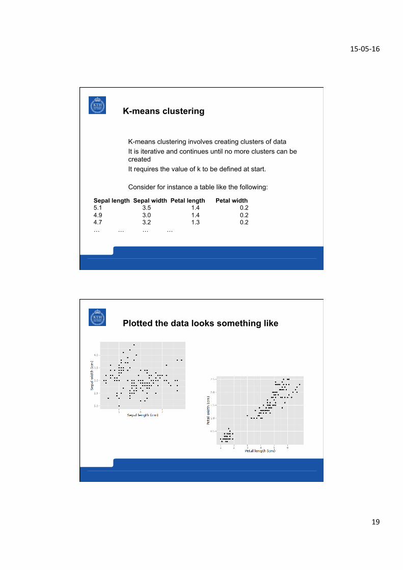
K-means clustering

K-means clustering involves creating clusters of data It is iterative and continues until no more clusters can be created It requires the value of k to be defined at start. Consider for instance a table like the following:

Sepal length Sepal width Petal length Petal width 5.1 3.5 1.4 0.2 4.9 3.0 1.4 0.2 4.7 3.2 1.3 0.2 … … … …

Plotted the data looks something like

15-‐05-‐16

20

K-means clustering (continued)

In k means clustering, first pick k mean points randomly in the space Caculate the distance from each object to the points Assign datapoint to its closest mean point Recalculate means Once ended, we have k clusters

k-Nearest Neighbour classification

Assuming instead a table like this where we have lables to ”clusters”

Sepal length Sepal width Petal length Petal width Species 5.1 3.5 1.4 0.2 iris setosa 4.9 3.0 1.4 0.2 iris setosa 4.7 3.2 1.3 0.2 iris setosa … … … … 7.0 3.2 4.7 1.4 iris versicolor … … … … … 6.3 3.3 6.0 2.5 iris virginica … … … … …

15-‐05-‐16

21

K-Nearest Neighbour algorithm

Given a new set of measurements, perform the following test: Find (using Euclidean distance, for example), the k nearest entities from the training set. These entities have known labels. The choice of k is left to us. Among these k entities, which label is most common? That is the label for the unknown entity.

In the OMIB example database

Sample 4984, and its neighbours

15-‐05-‐16

22

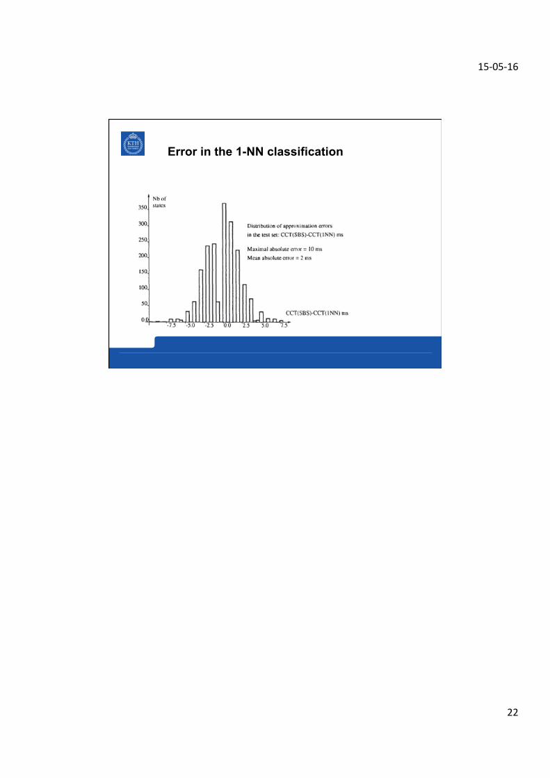
Error in the 1-NN classification

lecture #13 more machine learning - kth

Documents