Least-square mean effect: Application to the Analysis of SLR Time Series

D. Coulot1, P. Berio2, A. Pollet1

1. IGN/LAREG - Marne-la-Vallée – France

2. CNRS/OCA/GEMINI - Grasse - France

Contact: David.Coulot@ensg.ign.fr Fax: +33-1-64-15-32-53

Abstract

In this paper, we evidence an artifact due to the least square estimation method and, in particular, to the current modeling used to derive station position time series from space-geodetic measurements. Indeed, to compute such series, we in fact estimate constant (typically over one week) updates of station positions with respect to a priori models (ITRF2000, solid Earth tides, polar tide and oceanic loading effects). Thus, these estimations must underline the physical models which were not taken into account in the a priori modeling (atmospheric and hydrologic loading effects and even unknown signals, in our case).

As shown through the example of the Satellite Laser Ranging measurement processing, it is not the case: the weekly position time series exhibit weekly means of these physical signals but with a supplementary signal at the level of a few millimeters. This is the so-called “least square mean effect”.

To avoid this effect, alternative modeling such as periodic series can be used. A method to compute such periodic series for the station positions together with the geocenter motion is also presented in this paper.

Introduction

This paper comprises four parts. First of all, we present the least square mean effect from two points of view, theoretical and numerical. Secondly, we propose alternative models to reduce this effect. Then, we study a new method to process Satellite Laser Ranging (SLR) data. This method should help to use alternative modeling for a global network. Finally, we provide some conclusions and prospects.

1. Least square mean effect The quality presently reached by space-geodetic measurements allows us to study geodetic parameters (Earth Orientation Parameters (EOPs), station positions, Earth’s gravity field, etc.) under the form of time series. The modeling currently used to derive such time series is the following. The physical effects which are well understood are modeled (take as examples solid Earth tides or oceanic loading effects for station positions). These models are used to compute a priori values for the parameters worthy of interest and we compute the parameters with respect to these a priori values. These estimations are supposed to be constant over a given time (typically one day for EOPs and one week for station positions). And these estimations should help us to study the underlying physical effects (atmospheric loading effects, for instance). But, to do so, we need exact and judicious representations. We show that it is not really the case for the current modeling in this section.

1.1. Theoretical considerations

We consider a vector of physical parameters Xr

which vary with time. According to the modeling used, we split this vector in two parts: the modeled effects 0X

rand the effects we

want to study through time series Xr

δ , )()()( 0 tXtXtXrrr

δ+= .We know that the vector Xr

δ varies with time but, in order to get a robust estimation, we suppose it constant over a given

interval [ ]mtt ,1 . And, doing so, we hope that the constant estimations X̂r

δ will correspond to the averages of the underlying physical signals over this interval. The measurements used are modeled with a function f ( ),()( Xtftm

r≅ ) which is linearized

XtXtXftXtftm

rrr

rδ)).(,())(,()( 00 ∂

∂+≅ with ))(,( 0 tXt

Xf rr

∂∂ ,

the partial derivative matrix of f at the point ))(,( 0 tXtr

) to get the least square model. Furthermore, we can also linearize the measurements but with respect to the true signal to be

studied ( )()).(,())(,()( 00 tXtXtXftXtftm

rrr

rδ

∂∂

+≅ ).

As a consequence, on one hand, we have a relation between the measurements and the constant updates to be estimated and, on the other hand, a relation between these measurements and the true physical signal to be studied. From these two relations, we get the following observation equation:

)()).(,())(,()).(,())(,( 0000 tXtXtXftXtfXtXt

XftXtf

rrr

rrrr

rδδ

∂∂

+≅∂∂

+

This observation equation allows us to build the following system:

XAXA~

.~.rr

δδ ≅

with

⎥⎥⎥⎥⎥⎥⎥⎥⎥

⎦

⎤

⎢⎢⎢⎢⎢⎢⎢⎢⎢

⎣

⎡

∂∂

∂∂∂∂

=

))(,(

))(,(

))(,(

0

202

101

mm tXtXf

tXtXf

tXtXf

A

rr

M

rr

rr

,

⎥⎥⎥⎥⎥⎥⎥⎥⎥

⎦

⎤

⎢⎢⎢⎢⎢⎢⎢⎢⎢

⎣

⎡

∂∂

∂∂

∂∂

=

))(,(00

0))(,(0

00))(,(

~

0

202

101

mm tXtXf

tXtXf

tXtXf

A

rrL

MOMM

Lr

r

Lr

r

,

and .

⎟⎟⎟⎟⎟

⎠

⎞

⎜⎜⎜⎜⎜

⎝

⎛

=

)(

)()(

~2

1

mtX

tXtX

XrM

rr

δ

δδ

δ

r

This system is then used to compute the least square solution with a weight matrix P:

( ) )~~

.(~ˆ 1average

TTaverage XXAPAPAAXX

rrrrδδδδ −+≅

−

with and

⎟⎟⎟⎟⎟⎟⎟

⎠

⎞

⎜⎜⎜⎜⎜⎜⎜

⎝

⎛

=

X

XX

X

average

average

average

average

r

r

r

rM

δ

δδ

δ~

∫−=

mt

tmaverage

duuXttX

1

)(1

1

rrδδ .

In this solution, we can see that the estimations effectively contain the averages of the involved signals over the time interval but with a complementary term. We have called this term the “least square mean effect”.

1.2. Numerical examples

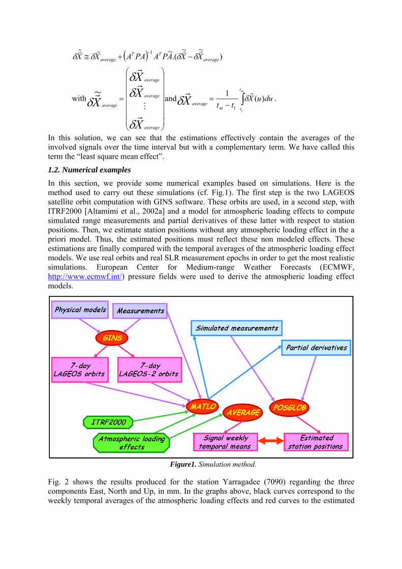
In this section, we provide some numerical examples based on simulations. Here is the method used to carry out these simulations (cf. Fig.1). The first step is the two LAGEOS satellite orbit computation with GINS software. These orbits are used, in a second step, with ITRF2000 [Altamimi et al., 2002a] and a model for atmospheric loading effects to compute simulated range measurements and partial derivatives of these latter with respect to station positions. Then, we estimate station positions without any atmospheric loading effect in the a priori model. Thus, the estimated positions must reflect these non modeled effects. These estimations are finally compared with the temporal averages of the atmospheric loading effect models. We use real orbits and real SLR measurement epochs in order to get the most realistic simulations. European Center for Medium-range Weather Forecasts (ECMWF, http://www.ecmwf.int/) pressure fields were used to derive the atmospheric loading effect models.

Figure1. Simulation method.

Fig. 2 shows the results produced for the station Yarragadee (7090) regarding the three components East, North and Up, in mm. In the graphs above, black curves correspond to the weekly temporal averages of the atmospheric loading effects and red curves to the estimated

weekly time series. The graph below shows the absolute differences between black and red curves, so the least square mean effects.

Table 1 provides maximum values of differences of a few millimeters (2 mm for the Up component). And, on average, the least square mean effect is approximately 10 % of the amplitude of the loading effects.

Figure 2. Simulation results for the station Yarragadee (7090).

Graphs above: black (resp. red) curves correspond to the weekly temporal averages of the atmospheric loading effects (resp. to the estimated weekly time series) in mm.

Graph below: absolute values of least square mean effects per component in mm.

Table 1. Statistics of the results shown on Fig. 2.

Values (mm) Minimum Maximum Average RMS East 2.37 10-4 1.26 0.15 0.13 North 1.86 10-5 0.95 0.13 0.12 Up 2.29 10-5 2.00 0.34 0.32

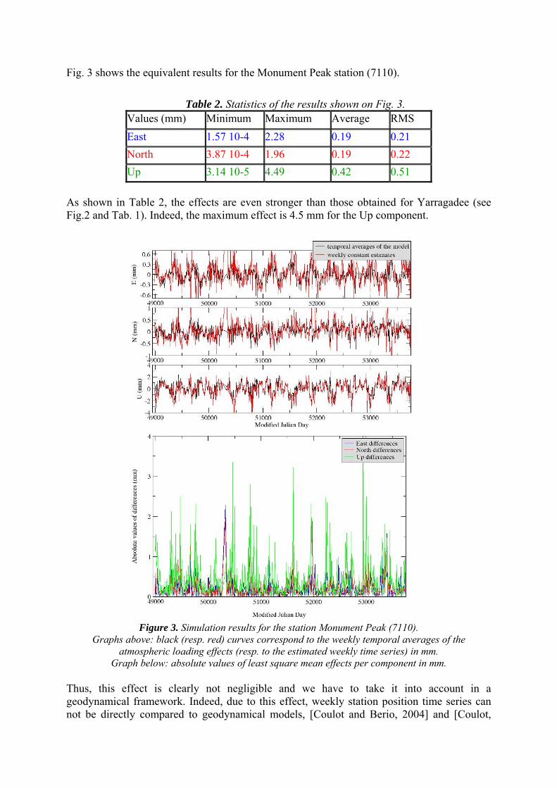
Fig. 3 shows the equivalent results for the Monument Peak station (7110).

Table 2. Statistics of the results shown on Fig. 3.

Values (mm) Minimum Maximum Average RMS East 1.57 10-4 2.28 0.19 0.21 North 3.87 10-4 1.96 0.19 0.22 Up 3.14 10-5 4.49 0.42 0.51

As shown in Table 2, the effects are even stronger than those obtained for Yarragadee (see Fig.2 and Tab. 1). Indeed, the maximum effect is 4.5 mm for the Up component.

Figure 3. Simulation results for the station Monument Peak (7110).

Graphs above: black (resp. red) curves correspond to the weekly temporal averages of the atmospheric loading effects (resp. to the estimated weekly time series) in mm.

Graph below: absolute values of least square mean effects per component in mm. Thus, this effect is clearly not negligible and we have to take it into account in a geodynamical framework. Indeed, due to this effect, weekly station position time series can not be directly compared to geodynamical models, [Coulot and Berio, 2004] and [Coulot,

2005]. Furthermore, the results provided in [Penna and Stewart, 2003], [Stewart et al., 2005], and [Penna et al., 2007] show that this effect could create spurious periodic signals in the estimated time series. To reduce this effect, we have studied some alternative models.

2. Alternative models

We have studied two alternative modeling. The first one uses periodic terms and the second one is based on wavelets.

2.1. Periodic series

The first model is a periodic one. Each of the three positioning componentsϕ is modeled as

periodic series: ∑=

+≅n

i ii

ii t

Tbt

Tat

1

)2sin()2cos()( ππϕ where the periods are the

characteristic periods of the involved signals. Instead of estimating weekly

niiT ,1)( =

ϕ time series, all available measurements are stacked to compute the coefficients and . niia ,1)( = niib ,1)( =

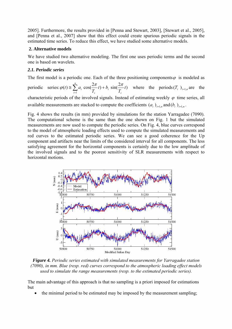
Fig. 4 shows the results (in mm) provided by simulations for the station Yarragadee (7090). The computational scheme is the same than the one shown on Fig. 1 but the simulated measurements are now used to compute the periodic series. On Fig. 4, blue curves correspond to the model of atmospheric loading effects used to compute the simulated measurements and red curves to the estimated periodic series. We can see a good coherence for the Up component and artifacts near the limits of the considered interval for all components. The less satisfying agreement for the horizontal components is certainly due to the low amplitude of the involved signals and to the poorest sensitivity of SLR measurements with respect to horizontal motions.

Figure 4. Periodic series estimated with simulated measurements for Yarragadee station

(7090), in mm. Blue (resp. red) curves correspond to the atmospheric loading effect models used to simulate the range measurements (resp. to the estimated periodic series).

The main advantage of this approach is that no sampling is a priori imposed for estimations but

• the minimal period to be estimated may be imposed by the measurement sampling;

• regarding unknown signals, it will probably be difficult to find the involved periods; • this model can difficultly take into account discontinuities such as earthquakes.

2.2. Wavelets To go further, we have also studied a model based on wavelets. We have used, as a first test, the simplest wavelet, Haar’s wavelet, for which the core function ψ is defined as follows:

⎪⎪⎪

⎩

⎪⎪⎪

⎨

⎧

<≤−

<≤

=

not if 0

121 if 1

210 if 1

)( t

t

tψ .

Each of the three positioning componentsϕ is modeled by the decomposition of the involved

physical signal on the wavelet basis: with ∑ ∑−= =

=2

1

max

0,, )()(

j

jj

n

nnjnj tat ψϕ

⎩⎨⎧ <−

=not if 0

0 if 12max

jn

j

and ⎟⎟⎠

⎞⎜⎜⎝

⎛ −= j

j

jnj

ntt

22

21)(, ψψ .

All available measurements are stacked to compute the coefficients . The discontinuities can now be taken into account with the help of this time-frequency representation.

nja ,

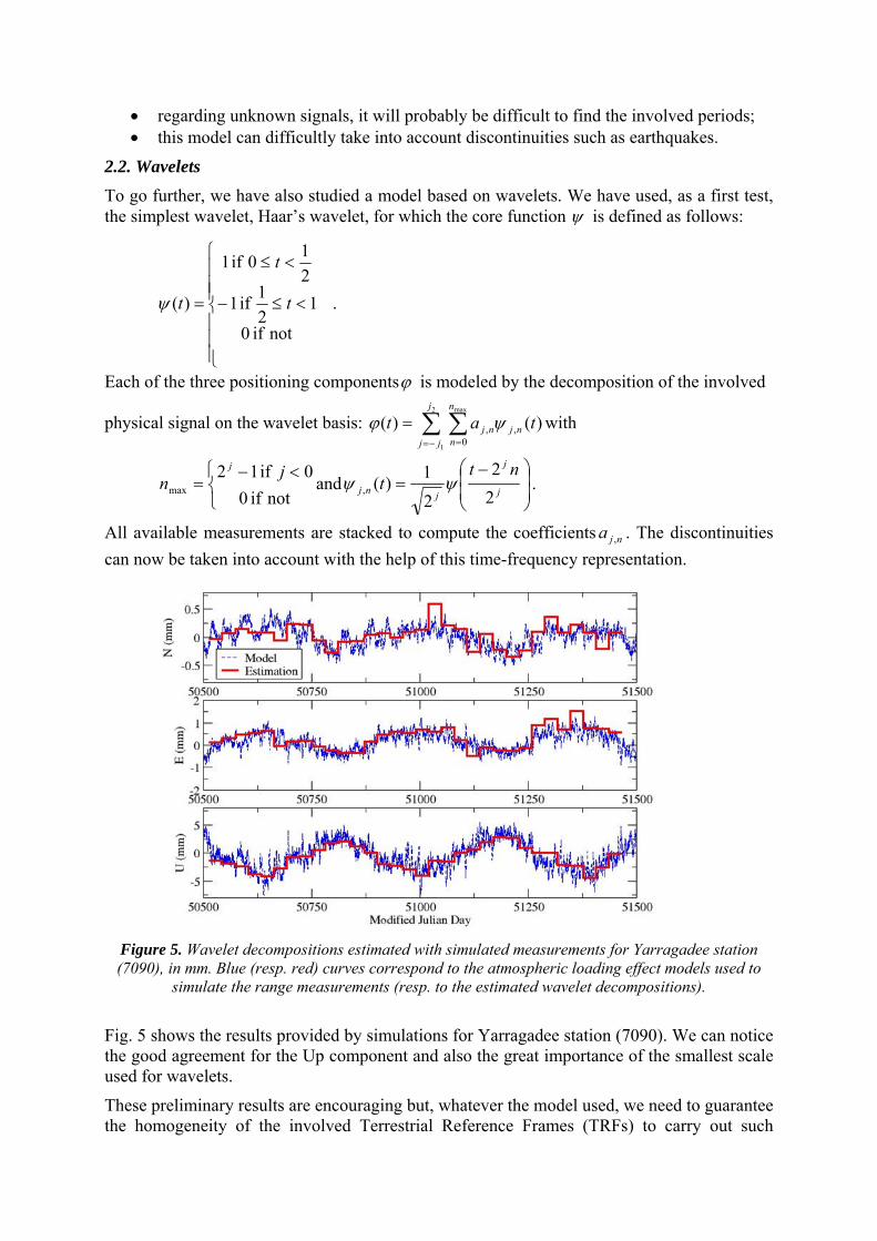
Figure 5. Wavelet decompositions estimated with simulated measurements for Yarragadee station (7090), in mm. Blue (resp. red) curves correspond to the atmospheric loading effect models used to

simulate the range measurements (resp. to the estimated wavelet decompositions).

Fig. 5 shows the results provided by simulations for Yarragadee station (7090). We can notice the good agreement for the Up component and also the great importance of the smallest scale used for wavelets.

These preliminary results are encouraging but, whatever the model used, we need to guarantee the homogeneity of the involved Terrestrial Reference Frames (TRFs) to carry out such

computations for a station network. Furthermore, we can take the opportunity of such global computation to derive geodynamical signals contained in global parameters such as translations. To reach this goal, we have developed a new approach to process SLR data [Pollet, 2006].

3. New model for SLR data processing

3.1. General considerations In the “classical approach”, the starting point is the observation system Y=A.δX composed by the pseudo measurements Y, the design matrix A and the parameters to be computed δX. By applying weak or minimum constraints, we are able to derive weekly solutions [Altamimi et al., 2002b] (usually, daily EOPs together with weekly station positions for the considered network). On the basis of these weekly solutions, with the help of Helmert’s transformation - here are the well-known formulae for station positions and for EOPs [Altamimi et al., 2002a]:

we can compute station positions in the a priori reference frame (ITRF2000, for instance) together with coherent EOPs and also 7-parameter transformation between involved TRFs.

The new model we have developed allows us to compute all these parameters in the same process, directly at the observational level. To derive this new approach, we have directly translated Helmert’s transformations at the level of the previous observation system: Y=A.δX with δX=δXC+T+DX0+RX0 and δEOP=δEOPC+εR{X,Y,Z}. Doing so, we have replaced the parameters δX and δEOP by new ones: δXC, T, D, R{X,Y,Z} and δEOPC.

Theoretical considerations and numerical tests with SLR data have shown that the rotations R{X,Y,Z} were not needed at all in this model. We did not keep them.

The normal matrices provided by this new approach present a rank deficiency of 7, coming from:

• the fact that SLR data do not carry any orientation information (deficiency of 3);

• the estimation of three translations and a scale factor (deficiency of 4).

This rank deficiency in fact corresponds to the definition of the totally unknown TRF underlying the estimated δXC for which the seven degrees of freedom need to de defined. To do so, minimum constraints [Sillard and Boucher, 2001] are applied with respect to the ITRF2000 and with the help of a minimum network.

3.2. First results In this section, we provide the preliminary results produced with this new model for SLR data processing over 13 years.

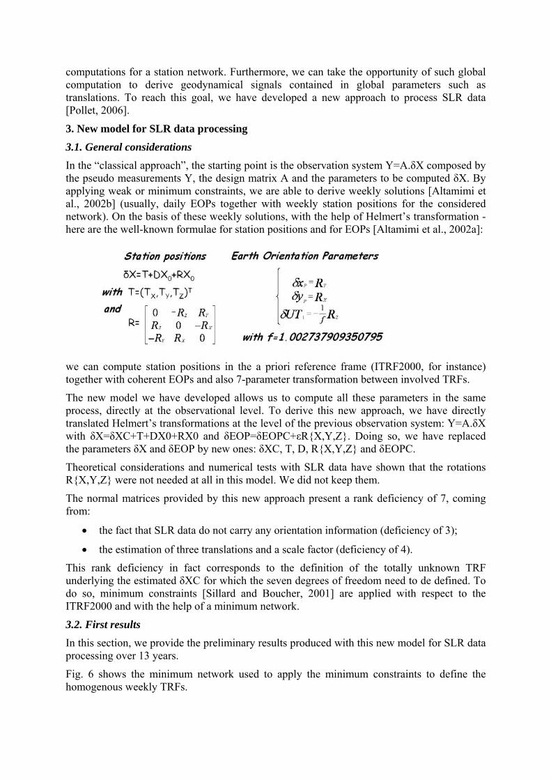
Fig. 6 shows the minimum network used to apply the minimum constraints to define the homogenous weekly TRFs.

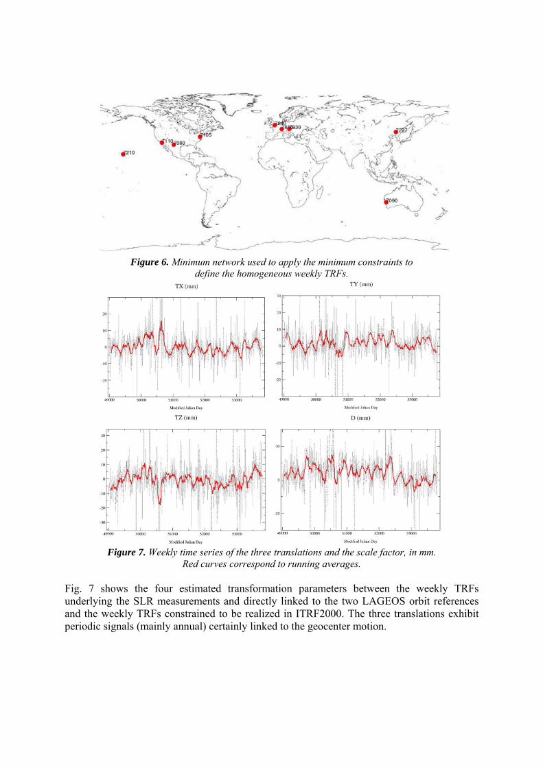
Figure 6. Minimum network used to apply the minimum constraints to

define the homogeneous weekly TRFs.

Figure 7. Weekly time series of the three translations and the scale factor, in mm.

Red curves correspond to running averages.

Fig. 7 shows the four estimated transformation parameters between the weekly TRFs underlying the SLR measurements and directly linked to the two LAGEOS orbit references and the weekly TRFs constrained to be realized in ITRF2000. The three translations exhibit periodic signals (mainly annual) certainly linked to the geocenter motion.

Figure 8. Results produced with the new method for EOPs and station positions. Graph up left: EOP

residuals (mas) with respect to EOPC04 time series [Gambis, 2004] consistent with the estimated station positions. Three other graphs: Mount Stromlo - 7849, in blue- and Yarragadee - 7090, in red-

station three positioning component estimated time series (cm).

Fig. 8 shows the results provided by the new method for EOPs and two Australian SLR stations, Mount Stromlo (blue curves) and Yarragadee (red curves). Regarding EOPs, the weighted biases (resp. the WRMS) are respectively 5µas for Xp and 23µas for Yp (resp. 280µas for Xp and Yp). Regarding the station position time series, we can notice the similarities between these series. The constant difference between the two Up time series is certainly due to range biases which were not taken into account for these computations.

3.3. Toward global estimations over long period

How this new model can help us to reduce the least square mean effect? We can replace the new parameters of the model by previous alternative models such as periodic series in the following example (new parameters to be estimated are underlined in green):

But, each harmonic estimated on station positions generates new rank deficiencies. Consequently, we have to generalize the minimum constraints for harmonic vectors. Furthermore, the number of involved parameters is very large (close to 50 000 in the next example).Thus, we have to use tools allowing the handling of large normal systems.

As a very preliminary computation, we have used this approach to compute amplitudes of annual signals contained in the four global parameters involved. The computation was carried out over 3 years of data. Amplitudes obtained are relatively satisfying (TX: 2.1 mm, TY: 3.6 mm, TZ: 1.1 mm and D: 0.9 mm). Moreover, the periodic series really absorb the annual signals as the annual harmonic totally disappears in the residual weekly parameters (the previous parameters called δZ0) computed with respect to this annual term.

4. Conclusions and Prospects All these results are satisfying but we of course need to go further by:

• using this periodic approach not only for global parameters but also for station positions;

• computing periodic series directly linked to oceanic loading effects together with series corresponding to atmospheric and hydrologic loading effects;

• deriving diurnal and semi-diurnal signals affecting EOPs with this approach;

• studying the spurious effects provided by this least square mean effect in the International Laser Ranging Service (ILRS) operational products.

We could also couple periodic series with more complex wavelet bases to get a more robust model and, eventually, with stochastic modeling in a filtering framework.

References [1] Altamimi, Z., P. Sillard, and C. Boucher: “ITRF2000: a new release of the International Terrestrial

Reference Frame for Earth science applications”, J. Geophys. Res., 107(B10), 2214, doi: 10.1029/2001JB000561, 2002a.

[2] Altamimi, Z., C. Boucher, and P. Sillard: “New trends for the realization of the International Terrestrial Reference System”, Adv. Space Res., 30(2), p. 175-184, 2002b.

[3] Coulot, D. and P. Berio: “Effet de moyenne par moindres carrés, application à l’analyse des séries temporelles laser”, Bulletin d’Information Scientifique & Technique de l’IGN, 75, p. 129-142, IGN (Eds), IGN-SR-03-083-G-ART-DC, 2004.

[4] Coulot, D.: “Télémétrie laser sur satellites et combinaison de techniques géodésiques. Contributions aux Systèmes de Référence Terrestres et Applications”, Ph. D. thesis, Observatoire de Paris, 2005.

[5] Gambis, D: “Monitoring Earth orientation using space-geodetic techniques: state-of-the-art and prospective”, J. Geod., 78, p. 295-305, 2004.

[6] Penna, N.T. and M.P. Stewart: “Aliased tidal signatures in continuous GPS height time series”, Geophys. Res. Lett., 30(23), p. 2184-2187, doi: 10.1029/2003GL018828, 2003.

[7] Penna, N.T., M.A. King, and M.P. Stewart: “GPS height time series: Short-period origins of spurious long-period signals”, J. Geophys. Res., 112, B02402, doi: 10.1029/2005JB004047, 2007.

[8] Pollet, A.: “Combinaison de mesures de télémétrie laser sur satellites. Contributions aux systèmes de référence terrestres et à la rotation de la Terre.”, Master research course report, Observatoire de Paris, 2006.

[9] Sillard, P. and C. Boucher: “Review of algebraic constraints in terrestrial reference frame datum definition”, J. Geod., 75, p. 63-73, 2001.

[10] Stewart, M.P., N.T. Penna, and D.D. Lichti: “Investigating the propagation mechanism of unmodelled systematic errors on coordinate time series estimated using least squares”, J. Geod., 79(8), p. 479-489, doi: 10.1007/s00190-005-0478-6, 2005.