learning lost temporal fuzzy association rules
TRANSCRIPT

Learning LostTemporal Fuzzy Association Rules
Stephen Gifford MatthewsBSc (Hons), MSc
A thesis submitted in partial fulfilment of
the requirements for the degree of
Doctor of Philosophy
at
De Montfort University
November 2012

Abstract
Fuzzy association rule mining discovers patterns in transactions, such as shopping baskets
in a supermarket, or Web page accesses by a visitor to a Web site. Temporal patterns can be
present in fuzzy association rules because the underlying process generating the data can be
dynamic. However, existing solutions may not discover all interesting patterns because of a
previously unrecognised problem that is revealed in this thesis. The contextual meaning of fuzzy
association rules changes because of the dynamic feature of data. The static fuzzy representation
and traditional search method are inadequate.
The Genetic Iterative Temporal Fuzzy Association Rule Mining (GITFARM) framework
solves the problem by utilising flexible fuzzy representations from a fuzzy rule-based system
(FRBS). The combination of temporal, fuzzy and itemset space was simultaneously searched with
a genetic algorithm (GA) to overcome the problem. The framework transforms the dataset to a
graph for efficiently searching the dataset. A choice of model in fuzzy representation provides
a trade-off in usage between an approximate and descriptive model. A method for verifying
the solution to the hypothesised problem was presented. The proposed GA-based solution was
compared with a traditional approach that uses an exhaustive search method. It was shown how
the GA-based solution discovered rules that the traditional approach did not. This shows that
simultaneously searching for rules and membership functions with a GA is a suitable solution for
mining temporal fuzzy association rules. So, in practice, more knowledge can be discovered for
making well-informed decisions that would otherwise be lost with a traditional approach.
Acknowledgements
I would like to thank my supervisors, Dr Mario A Gongora, Professor Adrian A Hopgood and
Dr Samad Ahmadi, for their support, guidance and encouragement. Furthermore, the staff and
students in the Centre for Computational Intelligence, at De Montfort University, have been a
fantastic community of stimulating researchers. I extend my gratitude to Dr Simon Miller and Dr
Benjamin N Passow for proof reading this thesis.
My family has been incredibly supportive throughout my PhD journey, so I am thankful to:
my father, Harry; my mother, Irene; and my brother, Chris.
I graciously acknowledge the Doctoral Training Account funding from the Engineering and
Physical Sciences Research Council.
i
Contents
Contents iv
List of Figures vi
List of Tables viii
Abbreviations x
1 Introduction 11.1 The Problem . . . . . . . . . . . . . . . . . . . . . . . . . . . . . . . . . . . . . 2
1.2 Research Hypothesis . . . . . . . . . . . . . . . . . . . . . . . . . . . . . . . . 4
1.3 Thesis Structure . . . . . . . . . . . . . . . . . . . . . . . . . . . . . . . . . . . 4
2 Literature Review 62.1 Computational Intelligence . . . . . . . . . . . . . . . . . . . . . . . . . . . . . 6
2.1.1 Fuzzy Logic . . . . . . . . . . . . . . . . . . . . . . . . . . . . . . . . 7
2.1.2 Evolutionary Computation . . . . . . . . . . . . . . . . . . . . . . . . . 9
2.1.3 Discussion . . . . . . . . . . . . . . . . . . . . . . . . . . . . . . . . . 14
2.2 Genetic Fuzzy System . . . . . . . . . . . . . . . . . . . . . . . . . . . . . . . 14
2.2.1 Fuzzy Rule-Based System . . . . . . . . . . . . . . . . . . . . . . . . . 14
2.2.2 Accuracy Versus Interpretability . . . . . . . . . . . . . . . . . . . . . . 18
2.2.3 Taxonomy . . . . . . . . . . . . . . . . . . . . . . . . . . . . . . . . . 20
2.2.4 Discussion . . . . . . . . . . . . . . . . . . . . . . . . . . . . . . . . . 23
2.3 Association Rule Mining . . . . . . . . . . . . . . . . . . . . . . . . . . . . . . 23
2.3.1 Data Mining . . . . . . . . . . . . . . . . . . . . . . . . . . . . . . . . 23
2.3.2 Association Rule Mining . . . . . . . . . . . . . . . . . . . . . . . . . . 25
2.3.3 Algorithms . . . . . . . . . . . . . . . . . . . . . . . . . . . . . . . . . 27
2.3.4 Data Representations . . . . . . . . . . . . . . . . . . . . . . . . . . . . 29
2.3.5 Types of Association Rule Mining . . . . . . . . . . . . . . . . . . . . . 29
2.3.6 Metaheuristic Approaches . . . . . . . . . . . . . . . . . . . . . . . . . 30
2.3.7 Discussion . . . . . . . . . . . . . . . . . . . . . . . . . . . . . . . . . 31
2.4 Temporal Association Rule Mining . . . . . . . . . . . . . . . . . . . . . . . . . 31
2.4.1 Inter-Transaction . . . . . . . . . . . . . . . . . . . . . . . . . . . . . . 32
ii

2.4.2 Intra-Transaction . . . . . . . . . . . . . . . . . . . . . . . . . . . . . . 33
2.4.3 Discussion . . . . . . . . . . . . . . . . . . . . . . . . . . . . . . . . . 37
2.5 Fuzzy Association Rule Mining . . . . . . . . . . . . . . . . . . . . . . . . . . 38
2.5.1 Quantitative Association Rule Mining . . . . . . . . . . . . . . . . . . . 38
2.5.2 Utility Association Rule Mining . . . . . . . . . . . . . . . . . . . . . . 39
2.5.3 Fuzzy Association Rule Mining . . . . . . . . . . . . . . . . . . . . . . 40
2.5.4 Discussion . . . . . . . . . . . . . . . . . . . . . . . . . . . . . . . . . 42
2.6 Temporal Fuzzy Association Rule Mining . . . . . . . . . . . . . . . . . . . . . 43
2.6.1 Academia . . . . . . . . . . . . . . . . . . . . . . . . . . . . . . . . . . 43
2.6.2 Industry . . . . . . . . . . . . . . . . . . . . . . . . . . . . . . . . . . . 44
2.6.3 Discussion . . . . . . . . . . . . . . . . . . . . . . . . . . . . . . . . . 45
2.7 Web Mining . . . . . . . . . . . . . . . . . . . . . . . . . . . . . . . . . . . . . 45
2.7.1 Data Cleaning and Preprocessing . . . . . . . . . . . . . . . . . . . . . 46
2.7.2 Computational Intelligence in Web Usage Mining . . . . . . . . . . . . . 47
2.7.3 Discussion . . . . . . . . . . . . . . . . . . . . . . . . . . . . . . . . . 48
3 Datasets 503.1 Synthetic . . . . . . . . . . . . . . . . . . . . . . . . . . . . . . . . . . . . . . 50
3.2 Real-World . . . . . . . . . . . . . . . . . . . . . . . . . . . . . . . . . . . . . 52
3.2.1 Data Cleaning . . . . . . . . . . . . . . . . . . . . . . . . . . . . . . . . 54
3.2.2 User and Transaction Identification . . . . . . . . . . . . . . . . . . . . 54
3.2.3 Preprocessing . . . . . . . . . . . . . . . . . . . . . . . . . . . . . . . . 55
3.3 Discussion . . . . . . . . . . . . . . . . . . . . . . . . . . . . . . . . . . . . . . 55
4 GITFARM Framework 574.1 Data Transformation . . . . . . . . . . . . . . . . . . . . . . . . . . . . . . . . 58
4.2 Model of Mamdani Fuzzy Rule-Based System . . . . . . . . . . . . . . . . . . . 60
4.2.1 Approximate . . . . . . . . . . . . . . . . . . . . . . . . . . . . . . . . 61
4.2.2 Descriptive . . . . . . . . . . . . . . . . . . . . . . . . . . . . . . . . . 62
4.3 Genetic Algorithm . . . . . . . . . . . . . . . . . . . . . . . . . . . . . . . . . 63
4.3.1 Chromosome . . . . . . . . . . . . . . . . . . . . . . . . . . . . . . . . 63
4.3.2 Fitness Evaluation . . . . . . . . . . . . . . . . . . . . . . . . . . . . . 65
4.3.3 Initialisation . . . . . . . . . . . . . . . . . . . . . . . . . . . . . . . . 68
4.3.4 Restart . . . . . . . . . . . . . . . . . . . . . . . . . . . . . . . . . . . 70
4.3.5 Crossover: Difference Check . . . . . . . . . . . . . . . . . . . . . . . . 70
4.3.6 Crossover: HybridCrossover . . . . . . . . . . . . . . . . . . . . . . . . 74
4.3.7 Iterative Rule Learning . . . . . . . . . . . . . . . . . . . . . . . . . . . 79
4.4 Discussion . . . . . . . . . . . . . . . . . . . . . . . . . . . . . . . . . . . . . . 80
5 Experimental Methodology 815.1 Comparative Analysis Framework . . . . . . . . . . . . . . . . . . . . . . . . . 81
5.1.1 Define Model and Parameters . . . . . . . . . . . . . . . . . . . . . . . 81
iii

5.1.2 Algorithm Execution . . . . . . . . . . . . . . . . . . . . . . . . . . . . 82
5.1.3 Rule Analysis . . . . . . . . . . . . . . . . . . . . . . . . . . . . . . . . 83
5.2 Variables . . . . . . . . . . . . . . . . . . . . . . . . . . . . . . . . . . . . . . 85
5.2.1 GITFARM Parameters . . . . . . . . . . . . . . . . . . . . . . . . . . . 85
5.2.2 FuzzyApriori Parameters . . . . . . . . . . . . . . . . . . . . . . . . . . 85
5.2.3 Linguistic Labels and Membership Function Parameters . . . . . . . . . 85
5.2.4 Size of Temporal Partitions . . . . . . . . . . . . . . . . . . . . . . . . . 86
5.2.5 Similarity Measures . . . . . . . . . . . . . . . . . . . . . . . . . . . . 86
5.2.6 Width . . . . . . . . . . . . . . . . . . . . . . . . . . . . . . . . . . . . 87
5.2.7 Rule Lengths in IRL . . . . . . . . . . . . . . . . . . . . . . . . . . . . 88
5.3 Discussion . . . . . . . . . . . . . . . . . . . . . . . . . . . . . . . . . . . . . . 88
6 Learning Lost Temporal Fuzzy Association Rules 896.1 Preliminary Results . . . . . . . . . . . . . . . . . . . . . . . . . . . . . . . . . 89
6.1.1 Evolving Rules . . . . . . . . . . . . . . . . . . . . . . . . . . . . . . . 89
6.1.2 Evolving Multiple Rules . . . . . . . . . . . . . . . . . . . . . . . . . . 92
6.2 Comparative Analysis . . . . . . . . . . . . . . . . . . . . . . . . . . . . . . . . 95
6.3 Varying the Number of Membership Functions . . . . . . . . . . . . . . . . . . 100
6.4 Analysis of Number of Transactions . . . . . . . . . . . . . . . . . . . . . . . . 106
6.5 Analysis of Number of Items . . . . . . . . . . . . . . . . . . . . . . . . . . . . 108
6.6 Discussion . . . . . . . . . . . . . . . . . . . . . . . . . . . . . . . . . . . . . . 110
7 Conclusions 1127.1 Summary . . . . . . . . . . . . . . . . . . . . . . . . . . . . . . . . . . . . . . 112
7.2 Conclusions . . . . . . . . . . . . . . . . . . . . . . . . . . . . . . . . . . . . . 113
7.3 Further Work . . . . . . . . . . . . . . . . . . . . . . . . . . . . . . . . . . . . 114
A List of publications by Stephen G. Matthews directly related to PhD 116
iv

List of Figures
1.1 Example membership functions . . . . . . . . . . . . . . . . . . . . . . . . . . 2
1.2 Example membership function occurring on intersection of two adjacent member-
ship functions in a temporal period of a dataset . . . . . . . . . . . . . . . . . . 3
2.1 Crisp set tall . . . . . . . . . . . . . . . . . . . . . . . . . . . . . . . . . . . . . 7
2.2 Fuzzy set tall . . . . . . . . . . . . . . . . . . . . . . . . . . . . . . . . . . . . 7
2.3 Example of a 2-tuple membership function . . . . . . . . . . . . . . . . . . . . . 9
2.4 Process of genetic algorithm . . . . . . . . . . . . . . . . . . . . . . . . . . . . 10
2.5 Pareto front for minimising two objectives . . . . . . . . . . . . . . . . . . . . . 12
2.6 Process of CHC (Cross-generational elitist selection, Heterogeneous re-combination,
and Cataclysmic mutation) . . . . . . . . . . . . . . . . . . . . . . . . . . . . . 13
2.7 Mamdani fuzzy rule-based system . . . . . . . . . . . . . . . . . . . . . . . . . 15
2.8 Comparison of descriptive and approximate Mamdani fuzzy rule-based system
features . . . . . . . . . . . . . . . . . . . . . . . . . . . . . . . . . . . . . . . 17
2.9 Process of Iterative Rule Learning . . . . . . . . . . . . . . . . . . . . . . . . . 22
3.1 Histogram of quantities of items ordered in every transaction in the Blue Martini
Software Point of Sale dataset . . . . . . . . . . . . . . . . . . . . . . . . . . . 53
4.1 Relationship between the GITFARM framework and the KDD Process . . . . . . 58
4.2 Example graph transformed from dataset in Table 4.1 . . . . . . . . . . . . . . . 59
4.3 Suitability of approximate and descriptive membership functions for accuracy and
interpretability . . . . . . . . . . . . . . . . . . . . . . . . . . . . . . . . . . . . 62
4.4 Soft constrained learning for membership function parameters in an approximate
rule . . . . . . . . . . . . . . . . . . . . . . . . . . . . . . . . . . . . . . . . . 65
4.5 Membership functions for approximately 4.5 and approximately 15 . . . . . . . . 67
4.6 Membership functions for low, medium and high . . . . . . . . . . . . . . . . . 67
5.1 Comparative analysis framework . . . . . . . . . . . . . . . . . . . . . . . . . . 82
5.2 Overlapping approximate/descriptive membership functions . . . . . . . . . . . 84
5.3 Example of two 2-tuple membership functions (s1, 0) and (s1, 0.5) . . . . . . . . 87
6.1 Best fitness during one run of the GITFARM framework with different rule lengths
(k) for approximate and descriptive models with EPA dataset and IBM dataset . 90
v

6.2 Box plots of temporal fuzzy support and confidence for approximate/descriptive
models of the GITFARM framework and FuzzyApriori (FA) for one run with
different datasets . . . . . . . . . . . . . . . . . . . . . . . . . . . . . . . . . . 94
6.3 Percentage of rules found with only the GITFARM framework and both
approaches with different numbers of membership functions . . . . . . . . . . . 103
6.4 Rules not discovered with FuzzyApriori and have a final temporal fuzzy support
greater than or equal to the minimum threshold with datasets with different
numbers of membership functions . . . . . . . . . . . . . . . . . . . . . . . . . 104
6.5 Arithmetic mean of execution times of IRL with different numbers of membership
functions . . . . . . . . . . . . . . . . . . . . . . . . . . . . . . . . . . . . . . 105
6.6 Arithmetic mean of percentage of rules discovered with the GITFARM framework
and FuzzyApriori, and GITFARM framework for datasets with different numbers
of transactions . . . . . . . . . . . . . . . . . . . . . . . . . . . . . . . . . . . . 107
6.7 Arithmetic mean of rules not discovered in FuzzyApriori and now have measures
greater than or equal to one or both minimum thresholds for datasets with different
numbers of transactions . . . . . . . . . . . . . . . . . . . . . . . . . . . . . . . 107
6.8 Arithmetic mean of execution times of IRL on datasets with different numbers of
transactions . . . . . . . . . . . . . . . . . . . . . . . . . . . . . . . . . . . . . 108
6.9 Percentage of rules found with only the GITFARM framework and both
approaches with different numbers of items . . . . . . . . . . . . . . . . . . . . 109
6.10 Rules not discovered in FuzzyApriori and have a final temporal fuzzy support
greater than or equal to the minimum threshold for datasets with varying numbers
of items . . . . . . . . . . . . . . . . . . . . . . . . . . . . . . . . . . . . . . . 110
6.11 Arithmetic mean of execution times of IRL with different numbers of items in
datasets . . . . . . . . . . . . . . . . . . . . . . . . . . . . . . . . . . . . . . . 110
vi
List of Tables
1.1 Example of fuzzy support measure of one rule for each day in a sample dataset . 3
2.1 A taxonomy to analyse the interpretability of linguistic FRBS (Gacto et al., 2011) 20
2.2 Example market basket dataset . . . . . . . . . . . . . . . . . . . . . . . . . . . 26
2.3 Horizontal, vertical and tabular data formats of the same example dataset . . . . . 28
2.4 Inter-transaction patterns . . . . . . . . . . . . . . . . . . . . . . . . . . . . . . 32
2.5 Transaction sequences for individual customers . . . . . . . . . . . . . . . . . . 33
2.6 Intra-transaction patterns . . . . . . . . . . . . . . . . . . . . . . . . . . . . . . 33
3.1 Parameters of the IBM Quest synthetic dataset generator . . . . . . . . . . . . . 50
3.2 Sample dataset from IBM Quest synthetic dataset generator . . . . . . . . . . . . 52
3.3 The first 4 records from the EPA dataset . . . . . . . . . . . . . . . . . . . . . . 53
3.4 Records removed with resource suffixes in HTTP request . . . . . . . . . . . . . 54
3.5 Example of transaction with identical URL items . . . . . . . . . . . . . . . . . 55
3.6 Example of calculating time spent on page . . . . . . . . . . . . . . . . . . . . . 55
4.1 Example dataset containing three items in vertical layout . . . . . . . . . . . . . 59
4.2 Example adjacency matrix transformed from example dataset in Table 4.1 . . . . 60
4.3 Example dataset for demonstrating fitness evaluation . . . . . . . . . . . . . . . 67
6.1 Percentage of rules with assigned rule lengths for IRL in the GITFARM
framework . . . . . . . . . . . . . . . . . . . . . . . . . . . . . . . . . . . . . 92
6.2 Results of approximate/descriptive GITFARM and FuzzyApriori (United States
Environmental Protection Agency (EPA) dataset: 0.0011 minimum temporal
fuzzy support and 0.5 confidence. IBM dataset: 0.01 minimum temporal fuzzy
support and 0.1 confidence) . . . . . . . . . . . . . . . . . . . . . . . . . . . . . 93
6.3 Analysis of temporal fuzzy support and confidence for rules discovered with the
approximate and descriptive models of GITFARM framework and the systematic
search with FuzzyApriori (FA) . . . . . . . . . . . . . . . . . . . . . . . . . . . 97
6.4 Rules discovered with the approximate and descriptive models of GITFARM
framework that were lost and are now greater than or equal to the threshold(s) . . 98
6.5 Number of rules found in FuzzyApriori when using different numbers of
membership functions . . . . . . . . . . . . . . . . . . . . . . . . . . . . . . . . 101
vii
6.6 Percentage of rules with assigned rule lengths for IRL with different numbers of
membership functions . . . . . . . . . . . . . . . . . . . . . . . . . . . . . . . . 101
6.7 Number of rules found in FuzzyApriori when using different numbers of
membership functions . . . . . . . . . . . . . . . . . . . . . . . . . . . . . . . . 102
6.8 Percentage of rules with assigned rule lengths for IRL on datasets with varying
numbers of transactions . . . . . . . . . . . . . . . . . . . . . . . . . . . . . . . 106
6.9 Number of rules discovered in FuzzyApriori . . . . . . . . . . . . . . . . . . . . 106
6.10 Percentage of rules with assigned rule lengths for IRL with varying number of
items in datasets . . . . . . . . . . . . . . . . . . . . . . . . . . . . . . . . . . . 108
6.11 Number of rules found in FuzzyApriori with varying number of items in datasets 109
viii

Abbreviations
ACS Ant Colony System.
BMS-POS Blue Martini Software Point of Sale.
CHC Cross-generational elitist selection, Heterogeneous re-combination, and Cataclysmic
mutation.
CI computational intelligence.
CRISP-DM CRoss Industry Standard Process for Data Mining.
DB data base.
DNF disjunctive normal form.
Eclat Equivalence CLASS Transformation.
EP Tree extended partial support tree.
EPA United States Environmental Protection Agency.
ET Tree extended target tree.
FARIM Fuzzy Apriori Rare Itemset Mining.
FFP-growth Fuzzy Frequent Pattern-growth.
FP-growth Frequent Pattern growth.
FP-tree Frequent Pattern tree.
FRBS fuzzy rule-based system.
FTDA Fuzzy Transaction Data-mining Algorithm.
GA genetic algorithm.
GCCL genetic cooperative-competitive learning.
ix
GFS Genetic Fuzzy System.
GITFARM Genetic Iterative Temporal Fuzzy Association Rule Mining.
HTTP Hypertext Transfer Protocol.
IRL Iterative Rule Learning.
ITAR Incremental Temporal Association Rule.
ITARM Incremental Temporal Association Rules Mining.
KB knowledge base.
KDD Knowledge Discovery in Databases.
KEEL Knowledge Extraction based on Evolutionary Learning.
MOEA multi-objective evolutionary algorithm.
NMEEF-SD Non-dominated Multiobjective Evolutionary algorithm for Extracting Fuzzy rules
in Subgroup Discovery.
NSGA-II nondominated sorting genetic algorithm II.
PCBLX-α parent centric BLX-α.
PPM Progressive Partition Miner.
PSO particle swarm optimisation.
RB rule base.
SPF Segmented Progressive Filter.
TID transaction ID.
TSK Takagi-Sugeno-Kang.
TWAIN TWo end AssocIation miNer.
URL uniform resource locator.
VEGA vector evaluated GA.
x

Chapter 1
Introduction
Advances in information technology have accelerated the collection, storage and processing of
various sources of data in recent decades (Manyika et al., 2011). To acquire useful information
from databases, the term Knowledge Discovery in Databases (KDD) has emerged (Piatetsky-
Shapiro, 1990). Data mining is one step of KDD where the goal is to discover knowledge that is
accurate, comprehensible and interesting (Freitas, 2002). Commercial benefit can be gained from
information about customer purchases and credit card transactions, to mention a few. Another
beneficiary is science where information about measurements, such as those from microarrays or
telescopes, can be used to help form hypotheses, and classify or segment data (Tan et al., 2005).
There are a variety of methods in data mining that discover different types of information.
Association rule mining (Agrawal et al., 1993) is one that discovers interesting correlations
between items in a database. Agrawal et al. mined association rules from a retail company’s
database. An example of a rule is one that says “20% of customers who purchased pizza also
purchased beer”.
There are two extensions to association rule mining that incorporate additional knowledge.
The challenges of the composition of the two extensions are investigated in this thesis. One
extension is fuzzy association rules that uses fuzzy sets. The quantities of items in an association
rule are represented with words such that they are more interpretable to a human. For example, a
fuzzy association rule could take the form “customers who purchased a large quantity of pizza also
purchased a medium quantity of beer”. The other extension is temporal association rule mining.
This type of association rule mining incorporates information about when the rules occur more
frequently in time. For example, “customers on a Monday morning who purchased pizza also
purchased beer”. This research investigates a problem with mining association rules that have
both fuzzy quantities and temporal features.
It is demonstrated how the traditional approach to mining association rules that are both
temporal and fuzzy does not discover all rules. The assumptions and decisions made in the
traditional approach limit the temporal fuzzy association rules that can be discovered. This thesis
proposes the Genetic Iterative Temporal Fuzzy Association Rule Mining (GITFARM) framework
that provides flexibility to allow for the discovery of rules that a traditional approach cannot.
The problem is now introduced with an example in Section 1.1, the research hypothesis is
defined in Section 1.2 and the structure of thesis is explained in Section 1.3.
1

1.1 The Problem
The composition of fuzzy quantities and temporal features in association rule mining presents an
interesting problem. Association rules that combine these features are referred to as temporal
fuzzy association rules. Association rules, temporal association rules and fuzzy association rules
will be introduced in Sections 2.3.2, 2.4 and 2.5.3 respectively. There is a traditional approach to
finding temporal fuzzy association rules that has a previously unrecognised problem.
The traditional method of finding fuzzy association rules is a two-stage process consisting of
the following ordered steps:
1. Define parameters (linguistic terms and membership function parameters).
2. Mine the rules using the parameters.
The parameters defined in the first stage are described in detail in the literature review; the
membership functions define how words, or linguistic terms, are used to describe quantities. For
example, Figure 1.1 shows the membership functions that describe three linguistic terms low,
medium and high.
5 10 15 200
0.5
1 low medium high
Quantity
Deg
ree
ofm
embe
rshi
p
Fig. 1.1. Example membership functions
Once these are defined, the parameters are then used for mining fuzzy association rules.
However, mining fuzzy association rules that occur more frequently across a finite duration of
time presents a new problem. The traditional approach for mining temporal fuzzy association
rules assumes the parameters are static. The membership functions, which determine the linguistic
terms, do not change throughout the duration of the whole dataset. The contextual meaning
of linguistic terms may change with factors such as seasonal weather, sports events (Saleh and
Masseglia, 2010), or unforeseen events, e.g., hurricanes (Leonard, 2005). For example, a low
quantity of beer on an average weekday may have a different meaning on the day of a sporting
event. A change in contextual meaning is not represented with static membership functions.
Different membership functions from those defined before the mining process may yield more
significant rules in some temporal periods of the dataset. More significant rules may be present
when a quantity is near to the intersection of membership function boundaries. It is for this reason
that traditional approaches to mining temporal fuzzy association rules can lose some interesting
rules. An example of how rules are lost is given. Some preliminaries are discussed in the literature
review. Such as fuzzy support, which measures the frequency (i.e., strength) of a rule and is
discussed in Section 2.5.3.
2
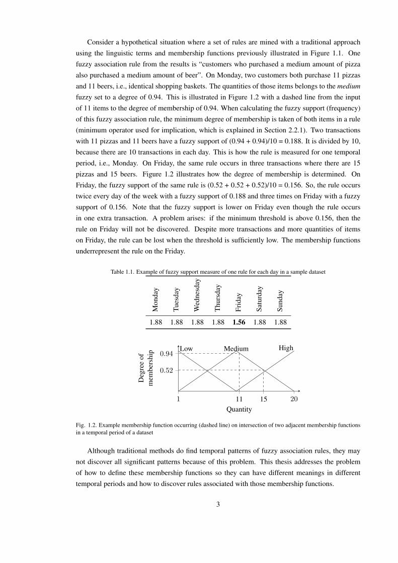
Consider a hypothetical situation where a set of rules are mined with a traditional approach
using the linguistic terms and membership functions previously illustrated in Figure 1.1. One
fuzzy association rule from the results is “customers who purchased a medium amount of pizza
also purchased a medium amount of beer”. On Monday, two customers both purchase 11 pizzas
and 11 beers, i.e., identical shopping baskets. The quantities of those items belongs to the medium
fuzzy set to a degree of 0.94. This is illustrated in Figure 1.2 with a dashed line from the input
of 11 items to the degree of membership of 0.94. When calculating the fuzzy support (frequency)
of this fuzzy association rule, the minimum degree of membership is taken of both items in a rule
(minimum operator used for implication, which is explained in Section 2.2.1). Two transactions
with 11 pizzas and 11 beers have a fuzzy support of (0.94 + 0.94)/10 = 0.188. It is divided by 10,
because there are 10 transactions in each day. This is how the rule is measured for one temporal
period, i.e., Monday. On Friday, the same rule occurs in three transactions where there are 15
pizzas and 15 beers. Figure 1.2 illustrates how the degree of membership is determined. On
Friday, the fuzzy support of the same rule is (0.52 + 0.52 + 0.52)/10 = 0.156. So, the rule occurs
twice every day of the week with a fuzzy support of 0.188 and three times on Friday with a fuzzy
support of 0.156. Note that the fuzzy support is lower on Friday even though the rule occurs
in one extra transaction. A problem arises: if the minimum threshold is above 0.156, then the
rule on Friday will not be discovered. Despite more transactions and more quantities of items
on Friday, the rule can be lost when the threshold is sufficiently low. The membership functions
underrepresent the rule on the Friday.
Table 1.1. Example of fuzzy support measure of one rule for each day in a sample dataset
Mon
day
Tues
day
Wed
nesd
ay
Thu
rsda
y
Frid
ay
Satu
rday
Sund
ay
1.88 1.88 1.88 1.88 1.56 1.88 1.88
1 11 15 20
0.52
0.94Low Medium High
Quantity
Deg
ree
ofm
embe
rshi
p
Fig. 1.2. Example membership function occurring (dashed line) on intersection of two adjacent membership functionsin a temporal period of a dataset
Although traditional methods do find temporal patterns of fuzzy association rules, they may
not discover all significant patterns because of this problem. This thesis addresses the problem
of how to define these membership functions so they can have different meanings in different
temporal periods and how to discover rules associated with those membership functions.
3

1.2 Research Hypothesis
The following hypothesis is the focus of this thesis.
“Traditional intra-transaction temporal fuzzy association rule mining algorithms may not discover
some rules because the degree of membership may occur at the intersection of membership
function boundaries. A fuzzy representation that provides flexibility in membership functions
is suitable for discovering these rules. The combination of a GA-based approach and flexible
fuzzy representation can discover fuzzy association rules, which exhibit intra-transaction temporal
patterns, that a traditional approach cannot.”
The traditional approach to intra-transaction temporal fuzzy association rule mining refers
to a search algorithm that uses an exhaustive and deterministic search method on membership
functions that are static/in-flexible and so do not change.
The GITFARM framework is created for mining intra-transaction temporal fuzzy association
rules. A GA is required to adapt a fuzzy representation so it is not static throughout the entire
dataset. A method for analysing the GA-based approach with a traditional approach is created.
Both real-world and synthetic datasets that have different dimensions are used to analyse the ability
to generalise and scale to different datasets.
1.3 Thesis Structure
The thesis is structured as follows:
• Chapter 2 surveys the literature that relates to the hypothesis. The background behind this
thesis’s core topics of computational intelligence (CI) and data mining is discussed. Specific
fields of literature focus on: the hybridisation of GAs and fuzzy logic, temporal association
rule mining and fuzzy association rule mining. Significant developments and state of the art
are discussed.
• Chapter 3 discusses a synthetic dataset generator and a real-world dataset. The features and
preprocessing of the datasets are described to provide an understanding of the type of data
and aid the justification of design decisions in the solution.
• Chapter 4 proposes a GA-framework for discovering intra-transaction temporal fuzzy
association rules. The framework is composed of multiple components: a data
transformation, a model of fuzzy representation, and a GA.
• Chapter 5 presents a comparative analysis framework that encompasses an experimental
methodology for analysing the GA-based framework.
• Chapter 6 presents a series of experiments designed to support the research hypothesis.
Preliminary results demonstrate the ability of the GA-based framework in finding rules.
The comparative analysis framework is then utilised to support the hypothesis.
4

• Chapter 7 briefly summarises this research, draws conclusions from the research, discusses
the conclusions and presents scope for future research.
5

Chapter 2
Literature Review
This thesis combines the fields of computational intelligence (CI) with data mining. Foundational
literature in both of these fields is presented to provide the required background knowledge. This
review sets the context of the field to enhance the accessibility for both the CI and data mining
communities. Key methods of CI and data mining are reviewed to understand previous work and
the relevance of this thesis.
The first section of this chapter, Section 2.1, introduces the CI methods used in this thesis.
Specifically, fuzzy logic and evolutionary computation. Section 2.2 provides an overview of the
hybridisation of CI methods used in this research referred to as Genetic Fuzzy Systems (GFSs).
Section 2.3 provides background information about data mining and focuses on association rule
mining. Section 2.4 reviews the temporal features of association rule mining and Section 2.5
reviews the fuzzy features of association rule mining. Section 2.6 highlights previous research
that tackles similar questions to this research.
2.1 Computational Intelligence
The question “Can machines think?” was posed by Turing (1950) when he introduced what is
now known as the Turing test for assessing a machine’s ability to exhibit intelligence. Artificial
intelligence is a broad field that has been defined by Hopgood (2005) as “the science of mimicking
human mental faculties in a computer”.
CI is a subfield of artificial intelligence (Bezdek, 1992) that aims to replicate intelligence in
machines using nature inspired methods. However, there is much debate about the definition of
the term CI and its interpretation can be considered subjective as discussed by Bezdek (2013)
who traced the origins of the term CI back to the 1970s. These methods are inspired from
observations of intelligent behaviour in the environment. The main areas of research in CI are
fuzzy logic, evolutionary computation and artificial neural networks. Fuzzy logic and evolutionary
computation are used in this thesis so these are introduced to provide preliminary knowledge
required for the literature review and the research.
6
2.1.1 Fuzzy Logic
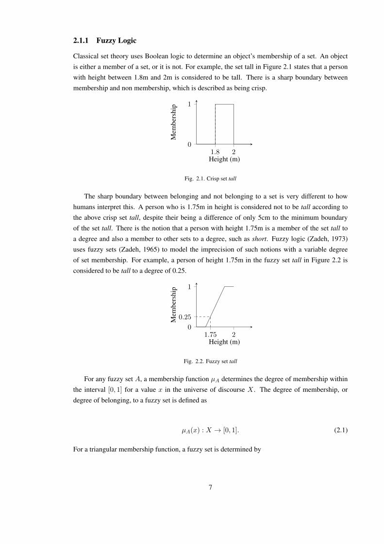
Classical set theory uses Boolean logic to determine an object’s membership of a set. An object
is either a member of a set, or it is not. For example, the set tall in Figure 2.1 states that a person
with height between 1.8m and 2m is considered to be tall. There is a sharp boundary between
membership and non membership, which is described as being crisp.
1.8 20
1
Height (m)
Mem
bers
hip
Fig. 2.1. Crisp set tall
The sharp boundary between belonging and not belonging to a set is very different to how
humans interpret this. A person who is 1.75m in height is considered not to be tall according to
the above crisp set tall, despite their being a difference of only 5cm to the minimum boundary
of the set tall. There is the notion that a person with height 1.75m is a member of the set tall to
a degree and also a member to other sets to a degree, such as short. Fuzzy logic (Zadeh, 1973)
uses fuzzy sets (Zadeh, 1965) to model the imprecision of such notions with a variable degree
of set membership. For example, a person of height 1.75m in the fuzzy set tall in Figure 2.2 is
considered to be tall to a degree of 0.25.
1.75 20
0.25
1
Height (m)
Mem
bers
hip
Fig. 2.2. Fuzzy set tall
For any fuzzy set A, a membership function µA determines the degree of membership within
the interval [0, 1] for a value x in the universe of discourse X . The degree of membership, or
degree of belonging, to a fuzzy set is defined as
µA(x) : X → [0, 1]. (2.1)
For a triangular membership function, a fuzzy set is determined by
7

µA(x) =
x−ab−a , if a ≤ x < b,
c−xc−b , if b ≤ x ≤ c,
0, otherwise.
(2.2)
where a, b and c are the parameters of the triangular membership function.
Fuzzy sets are suitable for problems with specific features. Vagueness and linguistic
uncertainty are present in words so fuzzy sets have been used to model the imprecision of notions,
concepts and perceptions used by humans. For example, there is uncertainty in low risk and high
risk loans issued by banks, and the perception of a hot temperature can be quite different between
humans. Imprecision is present in many physical system measurements, such as the measurement
of height. A measurement can be modelled with a fuzzy set to attempt to handle the imprecision.
Fuzzy numbers were introduced by Zadeh (1975) for approximating with real numbers that can
deal with the uncertainty and imprecision of quantities. A fuzzy number can model approximate
quantities such as the height of a person, e.g., about 1.7m, or the weight of fruit in a greengrocer,
e.g., approximately 0.5 kg. There is no linguistic term, such as low and high, associated with a
fuzzy number. A fuzzy number has a central point for modelling a number that has a maximum
degree of membership of 1 and the degree of membership for other numbers close to the central
number is reflected according to the proximity (Klir et al., 1997).
A fuzzy inference system utilises fuzzy logic in a FRBS. The description of FRBSs is
presented in the context of GFSs in Section 2.2.1 because the learning/tuning aspect of GFSs
is tightly coupled with FRBSs so they are discussed together.
2.1.1.1 The 2-tuple Linguistic Representation
The 2-tuple linguistic representation is an extension of the fuzzy representation previously
described in this chapter. The 2-tuple linguistic representation is described here because it forms
part of the solution presented in this thesis.
The 2-tuple linguistic representation is based on a symbolic translation of a fuzzy set and
has been introduced by Herrera and Martınez (2000). A symbolic translation is the lateral
displacement of the fuzzy set within the interval [−0.5, 0.5) that expresses the domain of a label
when it is displaced between two linguistic labels. The 2-tuple linguistic representation maintains
the shape of a fuzzy set whilst it is shifted left or right from its original membership function, but
not beyond the middle point between itself and a neighbouring membership function (dashed line
in Figure 2.3). The 2-tuple linguistic representation is defined as
{(sj , αj)|sj ∈ S, αj ∈ [−0.5, 0.5)}, (2.3)
where S represents a set of linguistic labels and α quantifies the lateral displacement of a linguistic
label within the interval [−0.5, 0.5) (the term α does not refer to an α-cut). Figure 2.3 is
8

an example of three membership functions, where s1 is laterally displaced to give a 2-tuple
membership function (s1,−0.3).
1 200
1s0 s2s1−0.5 0.5
α = −0.3
Deg
ree
ofm
embe
rshi
pFig. 2.3. Example of a 2-tuple membership function, (s1,−0.3) (light grey) that is displaced from s1 (dark grey)
The 2-tuple linguistic representation was proposed for computing with words. The
computational methods for computing with words can lose information and the 2-tuple linguistic
representation was used to overcome this limitation.
2.1.2 Evolutionary Computation
Evolutionary Computation is a broad field of CI that focuses on methods inspired by the principles
of natural selection and genetics. This section of the literature review introduces evolutionary
computation before focusing on the GA. However, other evolutionary computation algorithms are
also briefly discussed because of their application in the review of data mining. In this thesis, a
GA is the method for searching for temporal fuzzy association rules. Two variants of the classical
evolutionary computation model, i.e., a GA, are presented because they are important aspects used
in this thesis.
Following preliminary work in the 1950s and 1960s, the GA was introduced in Holland (1975).
Fogel (1998) discusses the history behind evolutionary computation. A GA is a search method
inspired by natural evolution of living organisms. Animals and plants have evolved over many
generations to reach a near-optimum state by modifying the genes of organisms and using natural
selection (Hopgood, 2012). A GA is a basic model of natural evolution that encodes a solution
to a problem in a chromosome. A population contains many chromosomes and the population
undergoes a series of steps defined in Figure 2.4.
The information in the genes of a chromosome is referred to as the genotype. The phenotype
is the observable characteristics of the chromosome in the environment. The positions of genes in
the chromosome are referred to as loci.
A GA starts by initialising a population with chromosomes. A chromosome traditionally
contains a bit string where each bit represents a variable in a given problem. Other chromosome
representations are possible, such as real values. Every chromosome’s ability as a solution to a
given problem is evaluated with a fitness function and a fitness value is assigned. Chromosomes
are then selected from the population at random, but more preference is given to the solutions that
have a better fitness value. For example, in roulette wheel selection, individuals are allocated slots
on a roulette wheel so that fitter individuals have more slots compared to weaker individuals that
9

have fewer slots. If elitism is used then the best individual is automatically copied to the new
population. Reproduction occurs with crossover and mutation, which are applied to the selected
chromosomes to modify them, and the resulting chromosomes are known as the offspring. The
offspring from reproduction form the new population, along with other selected chromosomes that
are copied into the new population. The new population is a new generation of solutions and the
whole process is repeated until the termination criteria are met.
Start
Initialise population
Evaluate fitness
Selection
Reproduction
Terminate?
Finish
Yes
No
Fig. 2.4. Process of genetic algorithm
The reproduction stage modifies parent chromosomes from the current population using either
crossover or mutation to produce offspring in the next population. The crossover operator splices
two chromosomes at one or more points in each chromosome. The spliced parts are swapped so
each chromosome contains genes of the other chromosome. The purpose of crossing over parts
of genes is to exploit parts of good chromosomes with the intention of creating better offspring.
Mutation operates on a single chromosome by randomly choosing one gene in the chromosome
and changing it to a random value. Mutation provides a mechanism for exploration of the search
space by introducing new solutions. Exploitation and exploration are essential aspects in many
evolutionary computation algorithms, such as a GA. In this thesis, a GA is used for mining
temporal fuzzy association rules.
There are other algorithms similar to GAs. A heuristic is a “rule of thumb” that is a means
for an educated guess or an informal judgement. A heuristic method provides a “good-enough
solution” to some complex problems that are otherwise difficult to solve. A metaheuristic was
introduced by Glover (1986), as a “meta-heuristic”. A metaheuristic is an upper level methodology
used to guide strategies in underlying heuristics for optimisation problems. A GA is in the category
of metaheuristic.
This is a classical model of a GA and there are many variants in evolutionary computation that
are suitable for different problems. For example, variations cited in this thesis are:
• Genetic programming (Koza, 1990) uses a tree structure to represent and evolve computer
programs.
10
• Grammatical evolution (Ryan et al., 1998) has a user-defined grammar (such as Backus-
Naur Form) to evolve solutions.
• Differential evolution (Storn and Price, 1995) mutates a candidate first to produce a trial
vector that is then used by the crossover operator to produce an offspring.
• Evolution strategies (Schwefel, 1965) are based on the concept of evolution where
parameters control evolution.
Other evolutionary computation paradigms can be found in Engelbrecht (2007). There are
two variations of a classical GA that are now described. The foundational literature on GAs has
focused on solving problems that have one objective to search/optimise, which are referred to as
single-objective evolutionary algorithms. The first variation is a GA for problems with multiple
objectives. The second variation is a single-objective evolutionary algorithm that applies genetic
operators in a very different manner to classical GAs.
2.1.2.1 Multi-Objective Evolutionary Algorithm
Many problems have two or more objectives, often competing, where a trade-off between these
objectives is required to solve a problem. For example, the time-cost trade-off is common in
many areas because something that can be done quickly incurs a higher cost, so a balance between
objectives is required. The origins of work that recognise this type of problem dates back many
centuries and covers fields such as economics and game theory (Coello et al., 2007). The focus of
this review covers the multi-objective optimisation problem using evolutionary algorithms.
Classical approaches to multi-objective optimisation aggregate fitness values from multiple
objectives into one function (Hopgood, 2012). If there is a preference towards a particular trade-
off, weights are applied to the appropriate components of the fitness function. This is known
as preference-based multi-objective optimisation (Deb, 2005) and was first used by Gass and
Saaty (1955). It is subjective and an understanding of the application is required to identify the
preference. It is also sensitive towards the preferences because these can yield very different
solutions. This approach is straightforward and finds one near-optimal solution.
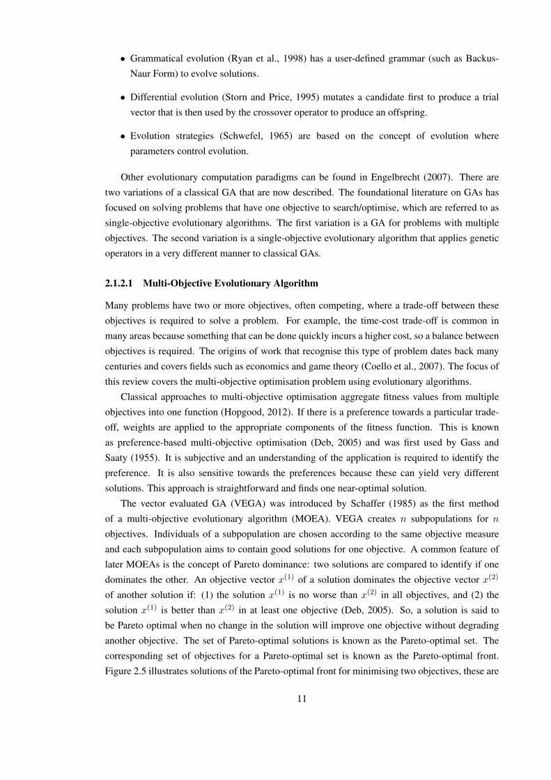
The vector evaluated GA (VEGA) was introduced by Schaffer (1985) as the first method
of a multi-objective evolutionary algorithm (MOEA). VEGA creates n subpopulations for n
objectives. Individuals of a subpopulation are chosen according to the same objective measure
and each subpopulation aims to contain good solutions for one objective. A common feature of
later MOEAs is the concept of Pareto dominance: two solutions are compared to identify if one
dominates the other. An objective vector x(1) of a solution dominates the objective vector x(2)
of another solution if: (1) the solution x(1) is no worse than x(2) in all objectives, and (2) the
solution x(1) is better than x(2) in at least one objective (Deb, 2005). So, a solution is said to
be Pareto optimal when no change in the solution will improve one objective without degrading
another objective. The set of Pareto-optimal solutions is known as the Pareto-optimal set. The
corresponding set of objectives for a Pareto-optimal set is known as the Pareto-optimal front.
Figure 2.5 illustrates solutions of the Pareto-optimal front for minimising two objectives, these are
11

indicated as the non-dominated solutions. The Pareto-optimal front is used by an expert to select
a solution that is most suitable for the given problem considering the trade-off.
Objective 1
Obj
ectiv
e2
Non-dominated solutionsDominated solutions
Fig. 2.5. Pareto front for minimising two objectives
2.1.2.2 CHC
The Cross-generational elitist selection, Heterogeneous re-combination, and Cataclysmic muta-
tion (CHC) algorithm was created by Eshelman (1991). CHC is reviewed because it is the
algorithm used in this thesis for mining temporal fuzzy association rules. The justification for
choosing CHC was made while reviewing the literature on fuzzy association rules as presented in
Section 2.5.3. The descriptions of each part of CHC’s abbreviation explain the key concepts of
CHC that distinguish it from a classical GA.
Cross-generational elitist selectionSelecting individuals for the next population occurs across parents and offsprings. This
selection method is the same as that used in the (µ+λ) evolutionary strategy (Schwefel,
1975) where µ refers to the number of parents and λ indicates the number of offspring.
Selection uses elitism to select the best µ parents from a population, or the best λ offspring,
and always copies these to the next population.
Heterogeneous re-combinationUniform crossover is applied where the probability of crossing over each bit in a binary
representation is 50%, rather than crossing over segments of bits. Uniform crossover is said
to be highly disruptive by Eshelman (1991) because it swaps about half the genes during
crossover. The incest prevention mechanism only performs crossover on chromosomes
whose measured difference is above a difference threshold. The Hamming distance
measures the number of positions in a bit string that are different. So when two individuals
are selected for crossover, the Hamming distance is measured and if the difference is
12

above the threshold then crossover is performed, otherwise it is not. The aim of the incest
prevention mechanism is to prevent reproduction between similar chromosomes.
Cataclysmic mutationThe mutation operator is not present in CHC. Instead, a restart operator provides the
exploration ability that is crucial for a GA. Restart reintroduces diversity when the
population converges and there have been no new chromosomes for multiple generations.
Instead of mutating every generation, a population is restarted in only those generations
where the level of diversity drops below a threshold, which is determined by the incest
prevention mechanism. Note that convergence is not used as a termination criterion. When
a population is restarted, each individual is reinitialised, except the best individual, which
is just copied. Each individual is evaluated and the algorithm continues. A Boolean
representation is used and a percentage of bits is flipped. The percentage of bits is referred to
as divergence rate (Eshelman, 1991). The best individual is used as a template for creating
other individuals.
The incest prevention mechanism helps to slow convergence and it is integral to CHC’s
operation because it influences crossover and restart. The difference threshold (d) is decremented
when there are no new chromosomes. Crossover uses the threshold to determine when to crossover
individuals based on their difference. Figure 2.6 illustrates the CHC algorithm with an emphasise
on its restart method.
Initialise population,initialise d = L/4
and evaluate
Crossover Evaluate
Select
If no new individualsThen d = d− 0.05(L/4)d < 0
Restart andinitialise d = L/4 No
Yes
Fig. 2.6. Process of CHC (Cross-generational elitist selection, Heterogeneous re-combination, and Cataclysmicmutation)
The difference threshold d is initialised to L/4. The numerator L is the length of bits in a
chromosome and so L represents the maximum difference between two chromosomes. To explain
the value of the difference threshold, it is recalled that CHC only crosses over chromosomes when
the parents are more than 50% different, i.e., more than L/2. Considering uniform crossover then
crosses over about half of the genes, which are known to be least 50% different, L/4 is half the
expected difference between parent chromosomes.
13

2.1.3 Discussion
CI has been presented and important areas of CI used in this thesis have been introduced. The
literature on fuzzy logic has introduced the basic concepts of fuzzy sets, linguistic terms and fuzzy
numbers. The application of fuzzy sets in fuzzy logic systems is described more in Section 2.2.1
in the context of a hybrid method that combines evolutionary computation and fuzzy logic. GAs
can be categorised as metaheuristics and this term is used throughout this literature review to
encompass similar search and optimisation methods. The classical GA and a variation of this,
CHC, are introduced to provide an understanding of the method that is central to this thesis.
2.2 Genetic Fuzzy System
The thesis focuses on the hybridisation of two CI methods: evolutionary computation and fuzzy
logic. Evolutionary computation is applied as a learning/tuning method to a fuzzy rule-based
system (FRBS). Aspects that are important to the design of a Genetic Fuzzy System (GFS) are
reviewed here, such as the accuracy-interpretability problem, taxonomy of a GFS application to a
FRBS and the various learning approaches.
The use of evolutionary computation for system identification of FRBSs has been very
successful and GFSs have been used for a variety of tasks such as fuzzy modelling, classification,
control and prediction (Herrera, 2008; Cordon, 2011).
2.2.1 Fuzzy Rule-Based System
Knowledge-based systems are used in artificial intelligence to store and use information
(Hopgood, 2012). Knowledge-based systems contain two components: a knowledge base (KB)
and an inference system. Knowledge is stored in a structured manner in the KB and the inference
system is explicitly separate from the knowledge. A FRBS is a type of knowledge-based system
that uses fuzzy rules in the KB. The principles of FRBSs are at the foundations of how this thesis
supports the hypothesis. The search method for temporal fuzzy association rules uses principles
taken from FRBSs. This section therefore reviews FRBSs.
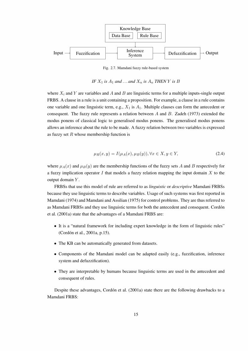
Mamdani (1974) introduced a Mamdani FRBS that uses fuzzy-rules, and fuzzification and
defuzzification components. Figure 2.7 shows the components of a Mamdani FRBS. The
fuzzification and defuzzification components are not present in a non-fuzzy knowledge-based
system, they are specific to a FRBS. Fuzzification maps the crisp values from the input domain to
fuzzy sets, and defuzzification performs the opposite operation of mapping fuzzy sets to crisp
output values. The inference system determines the fuzzy outputs from the fuzzy inputs by
applying an implication operator to each rule. Defuzzification then applies an aggregation operator
to produce a final fuzzy set that is then defuzzified to give a crisp output.
The KB stores the fuzzy rules in the rule base (RB) and the data base (DB)∗ contains the
linguistic terms and the associated fuzzy sets. Fuzzy rules have the following form∗DB refers to the collection of membership functions and linguistic terms. In this thesis it has a different meaning
to dataset.
14
Knowledge Base
Data Base Rule Base
InferenceSystemFuzzification DefuzzificationInput Output
Fig. 2.7. Mamdani fuzzy rule-based system
IF X1 is A1 and . . . and Xn is An THEN Y is B
where Xi and Y are variables and A and B are linguistic terms for a multiple inputs-single output
FRBS. A clause in a rule is a unit containing a proposition. For example, a clause in a rule contains
one variable and one linguistic term, e.g., X1 is A1. Multiple clauses can form the antecedent or
consequent. The fuzzy rule represents a relation between A and B. Zadeh (1973) extended the
modus ponens of classical logic to generalised modus ponens. The generalised modus ponens
allows an inference about the rule to be made. A fuzzy relation between two variables is expressed
as fuzzy set R whose membership function is
µR(x, y) = I(µA(x), µB(y)),∀x ∈ X, y ∈ Y, (2.4)
where µA(x) and µB(y) are the membership functions of the fuzzy sets A and B respectively for
a fuzzy implication operator I that models a fuzzy relation mapping the input domain X to the
output domain Y .
FRBSs that use this model of rule are referred to as linguistic or descriptive Mamdani FRBSs
because they use linguistic terms to describe variables. Usage of such systems was first reported in
Mamdani (1974) and Mamdani and Assilian (1975) for control problems. They are thus referred to
as Mamdani FRBSs and they use linguistic terms for both the antecedent and consequent. Cordon
et al. (2001a) state that the advantages of a Mamdani FRBS are:
• It is a “natural framework for including expert knowledge in the form of linguistic rules”
(Cordon et al., 2001a, p.15).
• The KB can be automatically generated from datasets.
• Components of the Mamdani model can be adapted easily (e.g., fuzzification, inference
system and defuzzification).
• They are interpretable by humans because linguistic terms are used in the antecedent and
consequent of rules.
Despite these advantages, Cordon et al. (2001a) state there are the following drawbacks to a
Mamdani FRBS:
15

• A lack of flexibility caused by the rigid partitioning of input and output spaces. Partitioning
refers to how linguistic terms cover the universe of discourse. A linguistic term is one
partition.
• Difficulties in finding the fuzzy partitions of input space when input variables are mutually
dependent.
• “The homogeneous partition of the input and output space does not scale well as the
dimensionality and complexity of input-output mappings increases” (Cordon et al., 2001a,
p.16).
• The size of the KB increases rapidly when the number of variables and linguistic terms
increases. An increase in linguistic terms provides finer granularity and enhances accuracy
but the system becomes less interpretable for humans.
There are two approaches that aim to overcome the shortcomings of descriptive Mamdani
FRBS by allowing more flexibility. The disjunctive normal form (DNF) fuzzy rule has a set of
linguistic terms that describe each variable (Gonzalez et al., 1994). A DNF fuzzy rule has the
form
IF X is A THEN Y is B
where the input variable X has a set of linguistic terms A and the output variable B has one
linguistic term B. The linguistic terms in A are joined by a disjunctive operator and this operator
provides flexibility in linguistic terms. The set of linguistic terms in a DNF fuzzy rule have the
form
A = {A1 or . . . or An}
Another model that allows more flexibility is the approximate Mamdani FRBS. An
approximate Mamdani FRBS has the same rule structure as a descriptive Mamdani FRBS but the
fuzzy sets are independent of each other. Rules in a descriptive Mamdani FRBS have linguistic
terms and the linguistic terms have the same meaning amongst rules. However, rules in an
approximate Mamdani FRBS each have their own meaning (Cordon and Herrera, 1995a). A rule
from an approximate Mamdani FRBS has the form
IF X is A THEN Y is B
where X and Y are variables and A and B are independent fuzzy variables. Where as a descriptive
Mamdani FRBS uses linguistic variables, an approximate Mamdani FRBS uses fuzzy variables
represented by fuzzy numbers. Rules from an approximate Mamdani FRBS are described as
being “semantic free” (Cordon et al., 2001a, p.18) because they have no linguistic label. For this
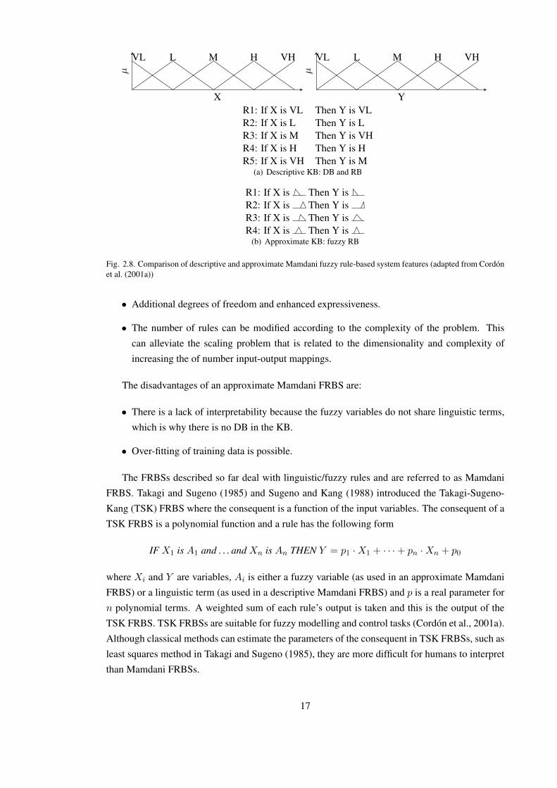
reason the KB does not contain a DB. Figure 2.8 illustrates the differences between the KBs of a
descriptive and an approximate Mamdani FRBS. According to Carse et al. (1996) the advantages
of an approximate Mamdani FRBS are:
16
VL L M H VH
X
µ
VL L M H VH
Y
µ
R1: If X is VL Then Y is VLR2: If X is L Then Y is LR3: If X is M Then Y is VHR4: If X is H Then Y is HR5: If X is VH Then Y is M
(a) Descriptive KB: DB and RB
R1: If X is Then Y isR2: If X is Then Y isR3: If X is Then Y isR4: If X is Then Y is
(b) Approximate KB: fuzzy RB
Fig. 2.8. Comparison of descriptive and approximate Mamdani fuzzy rule-based system features (adapted from Cordonet al. (2001a))
• Additional degrees of freedom and enhanced expressiveness.
• The number of rules can be modified according to the complexity of the problem. This
can alleviate the scaling problem that is related to the dimensionality and complexity of
increasing the of number input-output mappings.
The disadvantages of an approximate Mamdani FRBS are:
• There is a lack of interpretability because the fuzzy variables do not share linguistic terms,
which is why there is no DB in the KB.
• Over-fitting of training data is possible.
The FRBSs described so far deal with linguistic/fuzzy rules and are referred to as Mamdani
FRBS. Takagi and Sugeno (1985) and Sugeno and Kang (1988) introduced the Takagi-Sugeno-
Kang (TSK) FRBS where the consequent is a function of the input variables. The consequent of a
TSK FRBS is a polynomial function and a rule has the following form
IF X1 is A1 and . . . and Xn is An THEN Y = p1 ·X1 + · · ·+ pn ·Xn + p0
where Xi and Y are variables, Ai is either a fuzzy variable (as used in an approximate Mamdani
FRBS) or a linguistic term (as used in a descriptive Mamdani FRBS) and p is a real parameter for
n polynomial terms. A weighted sum of each rule’s output is taken and this is the output of the
TSK FRBS. TSK FRBSs are suitable for fuzzy modelling and control tasks (Cordon et al., 2001a).
Although classical methods can estimate the parameters of the consequent in TSK FRBSs, such as
least squares method in Takagi and Sugeno (1985), they are more difficult for humans to interpret
than Mamdani FRBSs.
17

Linguistic labels are often easily identifiable for applications, but when they are not, a domain
expert is used. To determine the membership functions for either Mamdani or TSK FRBSs there
are two broad approaches that are dependent on the FRBS application. The first is to manually
determine the membership functions from experts by determining the frequency of experts that
assert an object belongs to a group, or by asking experts to grade the degree of belonging of
an object (Dubois and Prade, 1980). The second method is to automatically determine the
membership functions from data with methods such as ad hoc data-driven methods, GAs and
artificial neural networks, to mention a few (Cordon et al., 2001a). Ad hoc data-driven methods
are supervised learning methods that use training data (discussed more in Section 2.3.1).
A domain expert is required for generating linguistic rules for a descriptive Mamdani FRBS. If
the domain expert cannot fully determine the KB then some aspect of learning either the linguistic
labels, fuzzy sets or rules is required. Cordon et al. (2001a) assert that an approximate Mamdani
FRBS can be generated in three ways. An approximate Mamdani FRBS can be generated directly
from a descriptive Mamdani FRBS by tuning the descriptive rules so they become approximate.
Another similar approach is that the rules are provided by a domain expert and the fuzzy sets
are learnt from data. The third approach is to use preliminary partitions of fuzzy sets provided
by the domain expert to constrain the learning process. This third approach has several types of
constraints for learning approximate FRBSs. A taxonomy of constrained learning was proposed
by Alcala et al. (2001). Constrained learning has two types of constraints. Hard constraints restrict
each parameter of a membership function to an interval (e.g., Cordon and Herrera (1995b)). Soft
constraints are more relaxed by restricting all parameters of a membership function to the same
interval (e.g., Cordon and Herrera (1997b)). Unconstrained learning imposes no restrictions on
the parameters of membership functions (e.g., Cordon and Herrera (1997a)). There is a trade-off
between the freedom of defining membership function parameters anywhere on the universe of
discourse (hard constrained learning) and the size of search space (unconstrained learning) (Alcala
et al., 2001). Soft constrained learning is a good trade-off between flexibility and size of the search
space.
FRBSs are referred to in the remaining parts of the literature review. FRBSs are drawn upon
when discussing the solution that this thesis proposes. There is a distinction between the type of
FRBS (TSK/Mamdani) and the Mamdani models (approximate/descriptive). Methods for defining
the linguistic labels, fuzzy sets and rules were also reviewed.
2.2.2 Accuracy Versus Interpretability
For modelling real-world systems there are two conflicting aims: creating a true model of
the system that is accurate and creating a model for humans to be able to understand that is
interpretable (Cordon, 2011). This problem is referred to as the accuracy-interpretability trade-off
(Casillas et al., 2003a,c). The accuracy-interpretability trade-off is an important consideration for
a GFS.
It is a challenging problem to achieve a good level of accuracy and also a good level of
interpretability. So, in practice, it is common for one of these features to take preference over the
18
other (Herrera, 2008). For a Mamdani FRBS there are two approaches to tackling the accuracy-
interpretability trade-off. One approach is to enhance the accuracy of a highly interpretable FRBS
(Casillas et al., 2003a,b); the other approach is to enhance the interpretability of a highly accurate
FRBS (Casillas et al., 2003c,d).
A descriptive Mamdani FRBS is suitable for maintaining interpretability because all fuzzy
sets are assigned linguistic labels in a rule. A TSK FRBS can achieve high accuracy because
of the degrees of freedom in the consequent (a polynomial function) and the availability of
numerical approximation methods to derive this, however, the consequent lacks interpretability.
An approximate Mamdani FRBS can also provide high accuracy because there is flexibility from
not having linguistic labels.
To assess these features of FRBSs, it is necessary to quantify them. Measures of accuracy
are well defined, for example, classification accuracy metrics the number of correctly classified
samples and regression typically uses mean square error. For interpretability there are many
measures that are subjective and this is still an open research question (Cordon, 2011). In recent
years there has been work that seeks to define the interpretability of FRBS and these are now
discussed.
Alonso et al. (2009) conducted an experiment to evaluate widely used interpretability indices.
A web poll with experts and non experts was setup to assess their views on different interpretability
measures for a specific problem. They concluded that a numerical index was not widely accepted
and this demonstrates the subjectivity of interpretability. They recommend a fuzzy index that
can be adapted to different situations and user preferences. Mencar and Fanelli (2008) have
defined a taxonomy of interpretability constraints for fuzzy sets, universe of discourse, fuzzy
information granules, fuzzy rules, fuzzy models and learning algorithms. Within the wider field of
fuzzy systems, Zhou and Gan (2008) created a taxonomy that includes low-level interpretability
and high-level interpretability. Low-level interpretability refers to the interpretability of the
membership functions whilst high-level interpretability refers to that of fuzzy rules. This
works serves to highlight surveys, frameworks and taxonomies of interpretability in FRBSs and
more broadly, fuzzy systems. Ishibuchi (2007) reviewed the use of MOEA in tackling the
accuracy-interpretability problem and highlighted different combinations of objectives designed
for interpretability. Comprehensive reviews of the many approaches to interpretability can be
found in Cordon (2011) and Gacto et al. (2011).
To date, the most comprehensive taxonomy of interpretability is found in Gacto et al. (2011).
Their taxonomy focuses on two dimensions of the meaning for interpretability. The first dimension
considers whether interpretability is semantic-based or complexity-based. Semantic-based
interpretability focuses on maintaining the semantics of membership functions and complexity-
based interpretability focuses on decreasing the complexity of models. The second dimension
considers the level at which interpretability refers to. It is either at the RB level or the fuzzy
partition level. Combining these dimensions creates four categories of interpretability in the
taxonomy of Gacto et al. (2011). The taxonomy of Gacto et al. is reproduced in Table 2.1, which
shows the four categories as quadrants of the table.
The taxonomy of interpretability of Gacto et al. (2011) is used throughout remaining chapters
19

Table 2.1. A taxonomy to analyse the interpretability of linguistic FRBS (Gacto et al., 2011)
Rule base level Fuzzy partition level
Q1 Q2
Complexity-based number of rules number of membership functionsinterpretability number of conditions number of features
Q3 Q4
Semantic-based consistency of rules completeness or coverageinterpretability rules fired at the same time normalisation
transparency of rule structure distinguishability(rule weights, etc.) complementaritycointension relative measures
of this thesis to describe the type of interpretability.
2.2.3 Taxonomy
This section presents a taxonomy of how GFSs can be applied to different areas of a FRBS. This
review will identify important aspects of using a GFS in this thesis. Herrera (2008) reviewed the
current literature and presented a refined taxonomy to that of previous taxonomies proposed in
Cordon et al. (2001b, 2004). The GFS taxonomy by Herrera (2008) has the following distinction
between the tasks of learning and tuning components of GFSs.
Genetic tuning Tuning a FRBS by tuning the DB but without altering the RB.
Genetic learning Learning KB components of a FRBS such as the RB or the DB.
The tuning and learning methods for GFSs are essential for the GA-based search method for
learning temporal fuzzy association rules. The principles of the tuning and learning methods are
the crucial aspect for the problem of learning lost rules, which was outlined in Section 1.1.
2.2.3.1 Tuning
Once a KB has been derived, a GFS can tune the DB of the FRBS to improve performance. This
can be achieved by tuning only the membership functions so they are optimised for the RB. This
was first applied to fuzzy logic controllers by Karr (1991a,b). This approach of tuning parameters
of derived membership functions is a common task of tuning GFSs. Crockett et al. (2006) extended
the parts of a FRBS that could be tuned by simultaneously tuning both the membership function
parameters and weights of fuzzy inference operators to achieve cooperation between fuzzy rules.
The weights of defuzzification operators have also been tuned (Kim et al., 2002). This reports on
the first methods that tune pre-defined components of a FRBS.
The RB is usually derived from heuristic knowledge of a domain expert. The heuristic
knowledge is usually valid independently of the environment, meaning that the RB model does
not change with the environment. Thus, the RB is considered to be a context-free model and the
meaning of the linguistic terms is context dependent (Botta et al., 2008b). For example, given a
20

rule “IF temperature is hot THEN fan speed is high” there may be different perceptions of the
term hot because of geographical location of domain experts. According to Gudwin and Gomide
(1994), psychologists have been interested in how context can effect perception of events, an
observation that also applies in the context of rules such as those above.
The context of fuzzy sets can be tuned so that the linguistic terms stay the same but the meaning
changes slightly in some context. This is another method of tuning a Mamdani FRBS (Cordon,
2011), which extends the discussion of tuning/learning GFSs from Section 2.2.3. The types of
methods for tuning the context of fuzzy sets are now reviewed.
Scaling the fuzzy set is an early approach to adapting the context pioneered by Gudwin and
Gomide (1994). The normalised universe of discourse [0, 1] is mapped to a contextualised universe
of discourse with a scaling function. The scaling function is tuned so the fuzzy sets for a variable
are tuned. Non-linear scaling has also been applied in Magdalena (1997).
Fuzzy modifiers have also been used to tune the context of fuzzy sets. A fuzzy modifier
maps a fuzzy set to another fuzzy set. Scaling a fuzzy set changes the partition of the universe
of discourse and fuzzy modifiers tune fuzzy sets while the partition of the universe of discourse
remains the same. Fuzzy modifiers have been implemented in the form of linguistic modifiers
such as extremely, very and more or less (De Cock and Kerre, 2000). Botta et al. (2008a) have
applied both scaling functions and fuzzy modifiers in a single framework.
The 2-tuple linguistic representation (discussed in Section 2.1.1.1) has been used by Alcala
et al. (2005, 2007) for lateral tuning of fuzzy sets. Rather than scaling or modifying a fuzzy
set, the fuzzy set is laterally displaced along the universe of discourse whilst maintaining the
membership function shape. Alcala et al. (2005, 2007) used a GA to tune the fuzzy sets to
achieve higher accuracy for a descriptive Mamdani FRBSs controller of a heating, ventilation,
and air conditioning system. The 2-tuple linguistic representation provides a reduction in the
search space because one parameter, α, is used to describe the membership function instead of
multiple parameters, e.g., parameters a, b and c for a triangular membership function. From the
perspective of the accuracy-interpretability trade-off, the 2-tuple linguistic representation reduces
the complexity-based interpretability at the fuzzy partition level because the dimensionality of
representing features is reduced (i.e., one parameter).
2.2.3.2 Learning
The other task of a GFS is to learn components of a FRBS. Thrift (1991) learnt the RB with a GA
for a fuzzy controller with a predefined DB. Some applications of FRBSs may produce many rules
that can be irrelevant, redundant, erroneous or contradictory. So, Ishibuchi et al. (1995) used a GA
to learn the significant rules for classification that were selected for the RB. As well as learning the
RB, the DB can also be learnt by two approaches. The a priori DB learning approach learns the
DB first using an evaluation measure and then a RB is derived from the DB. The embedded DB
learning approach incorporates the DB generation and RB generation into one step of the learning
process that is repeated (Filipic and Juricic, 1996; Glorennec, 1996; Ishibuchi and Murata, 1996).
Another use of genetic learning is to simultaneously learn both components of the KB: RB and
21
DB. Simultaneously evolving both membership functions and fuzzy rules in FRBSs is particularly
suitable for FRBS controllers (Homaifar and McCormick, 1995; Carse et al., 1996; Mucientes
et al., 2007), FRBS classifiers (Zhou and Khotanzad, 2007) and FRBS models (Delgado et al.,
1997; Cordon and Herrera, 2001). In these works the purpose of simultaneously evolving both the
definition of membership functions and induction of rules focuses more on improving accuracy
rather than interpretability.
GAs can be seen as either learning or optimisation algorithms as explained in Yao et al. (1996).
For learning, more than one solution in a population is used as there is much information present
in a population. For optimisation, there is only one optimal solution considered to be the best that
is the final result. The different approaches to learning are reviewed here.
In the context of machine learning there are two distinct approaches to applying a GA.
The Pittsburgh representation (Smith, 1980) represents a set of rules in one chromosome. A
Pittsburgh representation evolves the entire RB with one run of a GA. The first use of a Pittsburgh
representation specifically for a GFS was by Thrift (1991) and Carse et al. (1996). The Michigan
representation (Holland and Reitman, 1977) represents a single rule in one chromosome. The first
use of a Michigan representation specifically for a GFS was by Valenzuela-Rendon (1991). The
genetic cooperative-competitive learning (GCCL) approach is based on the Michigan approach
and the population represents the RB. The first use of a GCCL approach specifically for a GFS was
by Greene and Smith (1993). The RB is learnt by the chromosomes cooperating and competing in
a population.
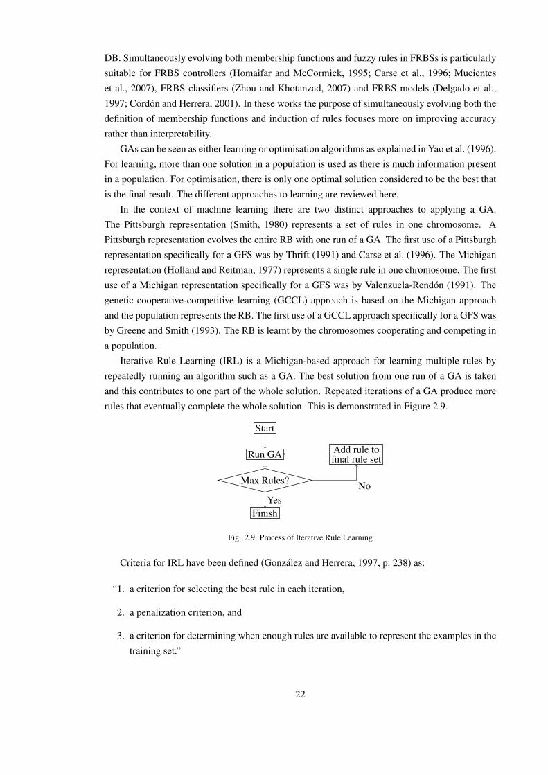
Iterative Rule Learning (IRL) is a Michigan-based approach for learning multiple rules by
repeatedly running an algorithm such as a GA. The best solution from one run of a GA is taken
and this contributes to one part of the whole solution. Repeated iterations of a GA produce more
rules that eventually complete the whole solution. This is demonstrated in Figure 2.9.
Start
Run GA
Max Rules?
Add rule tofinal rule set
Finish
NoYes
Fig. 2.9. Process of Iterative Rule Learning
Criteria for IRL have been defined (Gonzalez and Herrera, 1997, p. 238) as:
“1. a criterion for selecting the best rule in each iteration,
2. a penalization criterion, and
3. a criterion for determining when enough rules are available to represent the examples in the
training set.”
22
Gonzalez and Perez (1998) applied IRL to a classification problem where a GA is restarted
after a rule is discovered. Venturini (1993) used IRL with a steady state GA that continually
evolved classification rules whilst labelling the remaining examples as “uncovered”. The approach
by Venturini differs from typical IRL methods because the GA is not stopped, instead the same GA
continually runs. IRL has been used for fuzzy controllers by penalising rules that match existing
rules with same antecedent but different consequent (Herrera et al., 1995, 1998). Mata et al. (2002)
mined quantitative association rules and also penalised rules that have previously been covered.
The method in Shimada et al. (2006) used IRL by updating a pool of rules every generation.
2.2.4 Discussion
The hybridisation of GAs and fuzzy logic is a proven synergy of CI paradigms that is used in this
thesis.
The FRBS has been discussed in this section by expanding on the discussion of fuzzy logic
from Section 2.1.1. Different models of FRBSs systems have advantages and disadvantages that
are suitable for certain situations. Fuzzy association rule mining is not a FRBS because it has
no inference mechanism, but knowledge of FRBSs supports the design of fuzzy association rule
mining in this thesis.
The accuracy–interpretability problem is a trade-off between the two features when designing
a FRBS. There have been several taxonomies describing methods for tackling the accuracy–
interpretability problem and one of these taxonomies is used throughout the remainder of the
thesis.
The taxonomy of how GFSs are applied to the structure of FRBS highlights two key
paradigms: learning and tuning. Tuning FRBSs and context adaptation with the 2-tuples linguistic
representation have both been reviewed in Section 2.2.3.1. Learning has also been reviewed and
the simultaneous learning of membership functions and rules has been reviewed in Section 2.2.3.2.
Of particular interest to this thesis is the method for learning multiple rules by repeatedly iterating
a learning algorithm, i.e., IRL, because it is used in the solution that this thesis proposes.
2.3 Association Rule Mining
The CI methods relevant to this thesis have been reviewed and discussed. The other core field
of computer science that this thesis relates to is data mining. Data mining is reviewed first to
introduce the broad field. The review then focuses on a specific method of data mining, association
rule mining. The scope of the review narrows as temporal association rule mining and fuzzy
association rule mining are reviewed. CI methods from the previous section are now called upon
in multiple areas of the remaining review of literature.
2.3.1 Data Mining
Data mining is one step of KDD that extracts and identifies patterns in data. There are a variety
of methodologies and processes that define the steps in KDD, such as the KDD Process (Fayyad
23

et al., 1996a) and CRoss Industry Standard Process for Data Mining (CRISP-DM), to mention a
few. The KDD Process can be considered to be an academic methodology, whilst CRISP-DM
was created by a consortium of European companies. To understand the role of data mining, an
overview of the KDD Process is given. Whilst the KDD Process methodology is not as popular
as CRISP-DM, according to polls of practitioners (Piatetsky-Shapiro, 2002, 2004, 2007), it best
explains the key steps of KDD that are related to this research. The steps of the KDD Process are
reproduced from Fayyad et al. (1996b)† below.
“1. Developing an understanding of the application domain, the relevant prior knowledge, and
the goals of the end-user.
2. Creating a target data set: selecting a data set, or focusing on a subset of variables or data
samples, on which discovery is to be performed.
3. Data cleaning and preprocessing: basic operations such as the removal of noise or outliers
if appropriate, collecting the necessary information to model or account for noise, deciding
on strategies for handling missing data fields, accounting for time sequence information and
known changes.
4. Data reduction and projection: finding useful features to represent the data depending on
the goal of the task. Using dimensionality reduction or transformation methods to reduce
the effective number of variables under consideration or to find invariant representations for
the data.
5. Choosing the data mining task: deciding whether the goal of the KDD process is
classification, regression, clustering, etc.
6. Choosing the data mining algorithm(s): selecting method(s) to be used for searching
for patterns in the data. This includes deciding which models and parameters may be
appropriate (e.g. models for categorical data are different than models on vectors over
the reals) and matching a particular data mining method with the overall criteria of the
KDD process (e.g. the end-user may be more interested in understanding the model than its
predictive capabilities).
7. Data mining: searching for patterns of interest in a particular representational form or a
set of such representations: classification rules or trees, regression, clustering, and so forth.
The user can significantly aid the data mining method by correctly performing the preceding
steps.
8. Interpreting mined patterns, possible return to any of steps 1–7 for further iteration.
9. Consolidating discovered knowledge: incorporating this knowledge into the performance
system, or simply documenting it and reporting it to the interested parties. This also includes
checking for and resolving potential conflicts with previously believed (or extracted)
knowledge.ӠThe reproduced text does not include references to sections present in the original text.
24
The structure of this thesis, discussed in Section 1.3, follows the KDD process. Step 1 is
considered to be the literature review in this section that demonstrates our goal of mining temporal
fuzzy association rules. Steps 2 and 3 are discussed in Chapter 3 when the datasets are selected,
cleaned and preprocessed. Steps 4 to 7 are presented with the framework in Chapter 4 where the
dataset undergoes a transformation and decisions are made about how to run the framework. Steps
7 to 9 are covered by the results in Chapter 6.
When choosing a data mining task there are two aims, which relate to a user’s goals.
Descriptive tasks mine patterns that describe historical data and this is useful for exploring data.
Descriptive data mining methods are association rule mining and clustering. The other type of
data mining tasks are predictive tasks that mine patterns to make predictions and forecasts, such
as classification and regression (e.g., time series analysis).
Within the context of machine learning, data mining methods can also be classified according
to how data mining is performed. Supervised methods use training data that has a labelled target to
guide/supervise the learning process. For example, classification methods are trained to correctly
classify target classes before being tested on unseen data. Unsupervised methods learn patterns
from data without labelled targets. Association rule mining is in the category of unsupervised
learning. This is important because in Section 2.2.3 it was shown that GFSs are often used for
supervised learning tasks. But, in this thesis a GFS is used for an unsupervised learning task,
temporal fuzzy association rule mining.
This section has presented the KDD Process and explained the role of data mining in the KDD
Process. The descriptive and unsupervised nature of association rule mining has been explained
to identify how association rule mining can be categorised.
2.3.2 Association Rule Mining
Association rule mining is the process of identifying significant correlations between items in
transaction datasets (Agrawal et al., 1993). Association rule mining is commonly used for market
basket analysis to mine point-of-sale data from a shop, typically a supermarket. Each transaction
has a transaction ID (TID) and a list of purchased items that are present in a customer’s shopping
basket. The aim of market basket analysis is to learn about customer behaviour by discovering
common purchase patterns. This information can support businesses by informing actions such as
cross-marketing promotions (Olson and Delen, 2008), positioning stock on shelves (Power, 2002),
inventory management and customer relationship management (Tan et al., 2005), to mention a few.
An example of a market basket dataset is shown in Table 2.2. Association rules are expressed
as an implication of the form X ⇒ Y where the antecedent and consequent are sets of Boolean
items that are disjoint, i.e., X ∩ Y = ∅. The following rule could be mined from the example
dataset:
{pizza} ⇒ {beer}
A formal definition is presented. A dataset contains a set of N transactions T =
{t1, t2, ..., tN}. Each transaction comprises a subset of items, referred to as an itemset, from
25
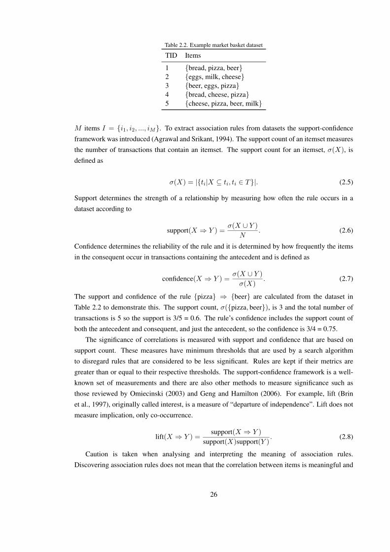
Table 2.2. Example market basket dataset
TID Items
1 {bread, pizza, beer}2 {eggs, milk, cheese}3 {beer, eggs, pizza}4 {bread, cheese, pizza}5 {cheese, pizza, beer, milk}
M items I = {i1, i2, ..., iM}. To extract association rules from datasets the support-confidence
framework was introduced (Agrawal and Srikant, 1994). The support count of an itemset measures
the number of transactions that contain an itemset. The support count for an itemset, σ(X), is
defined as
σ(X) = |{ti|X ⊆ ti, ti ∈ T}|. (2.5)
Support determines the strength of a relationship by measuring how often the rule occurs in a
dataset according to
support(X ⇒ Y ) =σ(X ∪ Y )
N. (2.6)
Confidence determines the reliability of the rule and it is determined by how frequently the items
in the consequent occur in transactions containing the antecedent and is defined as
confidence(X ⇒ Y ) =σ(X ∪ Y )
σ(X). (2.7)
The support and confidence of the rule {pizza} ⇒ {beer} are calculated from the dataset in
Table 2.2 to demonstrate this. The support count, σ({pizza, beer}), is 3 and the total number of
transactions is 5 so the support is 3/5 = 0.6. The rule’s confidence includes the support count of
both the antecedent and consequent, and just the antecedent, so the confidence is 3/4 = 0.75.
The significance of correlations is measured with support and confidence that are based on
support count. These measures have minimum thresholds that are used by a search algorithm
to disregard rules that are considered to be less significant. Rules are kept if their metrics are
greater than or equal to their respective thresholds. The support-confidence framework is a well-
known set of measurements and there are also other methods to measure significance such as
those reviewed by Omiecinski (2003) and Geng and Hamilton (2006). For example, lift (Brin
et al., 1997), originally called interest, is a measure of “departure of independence”. Lift does not
measure implication, only co-occurrence.
lift(X ⇒ Y ) =support(X ⇒ Y )
support(X)support(Y ). (2.8)
Caution is taken when analysing and interpreting the meaning of association rules.
Discovering association rules does not mean that the correlation between items is meaningful and
26

interesting (Han and Kamber, 2005). There may be a correlation between items that is coincidental
and meaningless within an application domain. Another interpretation of an association rule is
causality. An association rule means there is a strong occurrence of a set of items, but it does not
mean they are caused by those items. Association rule mining also requires more knowledge of
the application domain to ascertain causality.
2.3.3 Algorithms
Association rule mining is a well-established field with many algorithms. The Apriori algorithm
is reviewed here because an extension of the algorithm is used in this thesis. The extension
incorporates fuzzy set theory into the algorithm and this is discussed in Section 2.5.3. Other
Boolean association rule mining algorithms are reviewed to highlight suitability with certain
features of datasets.
2.3.3.1 Apriori
The Apriori‡ algorithm was introduced by Agrawal and Srikant (1994). Apriori allowed more than
one item in the consequent and Apriori was demonstrated to have better performance compared
to previous approaches (Agrawal et al., 1993). The Apriori method, and many others, use a two
stage process of:
1. Frequent Itemset Generation. This stage searches for all itemsets that have a support greater
than or equal to the minimum support threshold. Candidate itemsets that satisfy the support
threshold are referred to as frequent itemsets.
2. Rule Generation. This stage searches for all rules in the frequent itemsets that have
confidence greater than or equal to the minimum confidence threshold. Candidate rules
that satisfy the confidence threshold are referred to as strong rules.
Apriori is a breadth-first search algorithm that first discovers all frequent 1-itemsets (itemset
of size 1) then discovers the next size of itemset, i.e., 2-itemset, and increases the itemset size
until the search space is exhausted. Traversing the entire search space of itemsets is a large task
in itself that requires evaluating candidate itemsets. Agrawal and Srikant (1994) discovered that
the downward closure property (also referred to in literature as the Apriori principle and anti-
monotonicity) prunes the itemset generation of the search space and so reduces the number of
scans on the dataset when counting support of candidate itemsets. The downward closure property
states that if an itemset is frequent then all of its subsets are also frequent. Conversely, if an itemset
is infrequent then all of its subsets are also infrequent. The number of frequent itemsets that can be
generated with the Apriori algorithm is large so there are two compact representations from which
other frequent itemsets can be derived (Tan et al., 2005). A maximal frequent itemset is a frequent
‡The name of the algorithm, Apriori, is a noun that is based on the meaning of the Latin term a priori, which is anadjective that describes knowledge known ahead of time. The term Apriori is used throughout the thesis as the name ofthe algorithm.
27

itemset where none of its supersets are frequent. Maximal frequent itemsets allow pruning of the
search space for itemset generation. This method is based on a generate-and-test paradigm.
A data transformation in Apriori allows the efficiency of support counting for candidate
itemsets to be improved. The raw data is transformed into a hash tree data structure where nodes
contain items and leaf nodes represent a set of candidate itemsets that have common prefixes.
When counting support, the itemsets contained in each transaction are enumerated in a prefix tree.
The support counts of matching candidate itemsets are incremented.
2.3.3.2 FP-growth
Frequent Pattern growth (FP-growth) (Han et al., 2000) is a depth-first search algorithm that uses
a condensed representation of the data, a Frequent Pattern tree (FP-tree). The first stage scans the
dataset to construct the FP-tree, which is an extended prefix tree that contains support counts of
itemsets. The second stage searches for and extracts frequent itemsets directly from the FP-tree.
FP-growth differs from the generate-and-test paradigm used by the Apriori algorithm. A divide-
and-conquer strategy splits the problem into smaller subproblems and searches the tree from the
bottom up. The FP-tree is more suited to sparse datasets that have few items per transaction.
2.3.3.3 Eclat
A different approach to support counting is used in Equivalence CLASS Transformation (Eclat)
(Zaki, 2000). The Apriori and FP-growth algorithms mine frequent itemsets from datasets that are
in a horizontal data format. A horizontal data format identifies a row of itemsets in a transaction
using the TID, whilst the vertical data format lists all TIDs for each item. Table 2.3 illustrates both
formats and another common format, tabular.
Table 2.3. Horizontal, vertical and tabular data formats of the same example dataset
(a) Horizontal layout
TID Items
1 {A, B, C}2 {B, D, E}3 {A, C, D}4 {A, B, E}5 {A, B, D, E}
(b) Vertical layout
A B C D E
1 1 1 2 23 2 3 3 54 45 5
(c) Tabular layout
TID A B C D E
1 1 1 1 0 02 0 1 0 1 13 1 0 1 1 04 1 1 0 0 15 1 1 0 1 1
Intersection counting is a method for counting support on a vertical data format. Lists of
TID for items in a candidate itemset are joined to determine the number of shared TID to give a
support count. Similar to FP-growth, a depth-first search is performed. Eclat is more suited to
dense datasets with many items in each transaction because this is best represented with a vertical
data format.
28
2.3.3.4 Partition
Partition (Savasere et al., 1995) also uses vertical data format with a breadth-first search. Partition
splits the dataset into several logical non-overlapping partitions. Each partition is transformed into
a vertical data format and locally frequent itemsets are generated. The final stage scans the dataset
to check that locally frequent itemsets are also globally frequent.
2.3.4 Data Representations
Data representations are of crucial importance for algorithms, because there is a synergy between
a search algorithm and its data representation. A data transformation forms part of the solution
proposed in this thesis. Existing methods that use data representations for association rule mining
are reviewed here.
Tree structures are commonly used in association rule mining (Yan et al., 2007). A hash
tree (Agrawal and Srikant, 1994), a FP-tree (Han et al., 2000), and a P-tree and a T-tree
(Goulbourne et al., 2000; Coenen et al., 2004a) were applied to efficiently count support for
Boolean association rules. A generalised tree structure is an acyclic directed graph that provides
a suitable schema for representing the downward closure property (Agrawal and Srikant, 1994)
(discussed in Section 2.3.3.1).
Graphs have previously been used for association rule mining in the DLG algorithm (Yen
and Chen, 1996) and Similis (Cavique, 2004). Cavique (2004) transformed the dataset into an
undirected graph with the method from Chen et al. (2001) and formulated the market basket
problem as a maximum weighted clique problem (Bomze et al., 1999). The Primal-Tabu algorithm
(a metaheuristic) searches for cliques that represent rules. A grammar-based genetic programming
method for association rule mining aims to prevent producing invalid candidate solutions that are
not in the dataset (Luna et al., 2010b).
Graph data structures provide a suitable and natural representation of networks. Holme and
Saramaki (2012) have reviewed temporal networks and identified a class of graphs called contact
sequences. An edge of a contact sequence is a triple containing two vertices and a non-empty list
of time contacts. The time contacts are timestamps representing when contact is made between
two vertices. Although Holme and Saramaki (2012) do not focus on association rule mining, the
class of graphs referred to as contact sequences are relevant to the data structure used in this thesis
and a similar data structure is discussed in Section 4.1.
2.3.5 Types of Association Rule Mining
Association rule mining is a broad task and there are multiple variations of Boolean association
rule mining, some of which have subtle differences. A variety of association rules can be mined
from different datasets or for different purposes. Two types of association are combined in this
thesis so other commonly used types of association rule mining are reviewed. The purpose is to
define the boundaries of what type of association rule is the focus of this thesis.
29

2.3.5.1 Generalised/Multiple-Level Association Rule Mining
Srikant and Agrawal (1995) and Han and Fu (1995) both disseminated work at the same conference
that extended association rules by incorporating a taxonomy of items. Han and Fu (1995)
introduced multiple-level association rule mining, whilst Srikant and Agrawal (1995) introduced
generalised association rule mining. This allows more generalised association rules, such as
“people who buy outerwear tend to buy shoes” (Srikant and Agrawal, 1995).
2.3.5.2 Weighted Association Rule Mining
Cai et al. (1998) assign weights to items in a rule to assign more importance to those rules. The
weights are entirely application and end-user dependent.
2.3.5.3 Associative Classification Rule Mining
Liu et al. (1998) created a classifier using association rule mining where the consequent is limited
to a target class. Class association rules are mined from a training dataset and pruned to prevent
overfitting before used as a classifier.
2.3.5.4 Mining Multiple Minimum Supports
Mining association rules with multiple minimum supports of items can yield rules that have
different frequencies of items or items that are of a different nature (Liu et al., 1999). For example,
the sale of items such as champagne or microwaves occurs less frequently than beer or pizza.
Minimum support values are assigned to each item and the Apriori algorithm was extended.
2.3.5.5 Negative Association Rule Mining
Negative association rules (Savasere et al., 1998) search for rules that contain associations between
items that are sold and items that are not. For example, a negative association rule could be “5%
of customers who purchase pizza do not purchase water”.
2.3.6 Metaheuristic Approaches
The Boolean association rule mining algorithms that have been reviewed here employ exhaustive
methods. This thesis proposes the use of a metaheuristic for a specific type of association rule.
Metaheuristics for other particular types of association rule mining are briefly reviewed here. A
review of all types of association rule mining that focuses on evolutionary algorithms can be found
in del Jesus et al. (2011).
Kuo et al. (2007) clustered a dataset with an Ant Colony System (ACS) and then applied
ACS to mine association rules. ACS is a search method based on ants’ behaviours that seeks
to find a path between a colony and a food source. Kuo et al. demonstrate their approach
could be suitable for larger datasets. Another swarm intelligence method for association rule
mining is particle swarm optimisation (PSO) (Kuo et al., 2011). PSO has a population (swarm)
30

of solutions (particles) that moves through the search space by controlling particles’ positions
and velocities. Kuo et al. applied PSO to improve the efficiency of association rule mining and
automatically determine threshold values. A grammar-based approach is presented in Luna et al.
(2010a). Grammar-guided genetic programming searches for association rules by using genetic
programming to represent the rule in a tree structure and a grammar to specify the tree’s schema.
Ghosh and Nath (2004) extracted association rules with a Pareto-based MOEA that has
objectives for support count, comprehensibility and interestingness. Ghosh and Nath treated
the mining problem as a multi-objective problem because some objectives are conflicting. For
example, a rule may have lower support but be very interesting to the end-user. Dehuri et al. (2006)
use a MOEA parallelised across a cluster of workstations with three objectives: comprehensibility,
confidence and interestingness. Another multi-objective approach has been used in Nasiri et al.
(2010) but with simulated annealing. Simulated Annealing models the excitation of particles in
metals when they are heated to search for association rules.
Yan et al. (2005) applied IRL with a GA for mining Boolean association rules. An important
aspect of the approach by Yan et al. (2005) is that it does not require the minimum threshold values
to be specified, so Yan et al. refer to this approach as being database-independent.
2.3.7 Discussion
The broad area of knowledge discovery has been introduced. A knowledge discovery methodology
has been identified and is used later in this thesis. The task of association rule mining is
fundamental to this thesis and the Apriori algorithm has been introduced because this forms the
basis of the temporal fuzzy association rule mining algorithm. Association rule mining algorithms
that are seminal in the field were reviewed because the algorithms are suitable for datasets with
certain features. Other types of association rule mining were given a brief overview to distinguish
other types of rule. Metaheuristic methods for Boolean association rule mining were discussed
to identify the suitability of metaheuristics. This is important because the solution proposed in
this thesis searches for items in a rule. A variety of metaheuristic methods have been applied
and MOEAs are common for finding a trade-off in rule metrics. Graphs and trees are two
common data representations that were reviewed. The data representations are also used for
temporal, quantitative and fuzzy association rule mining, which is reviewed later in this chapter.
In particular, the contact sequence graph that incorporates temporal information is relevant to the
data transformation used in this thesis.
2.4 Temporal Association Rule Mining
The fundamentals of association rule mining have been introduced in the previous section. The
hypothesised problem is caused by the composition of temporal and fuzzy association rules. The
temporal aspect of association rule mining is discussed here.
Temporal association rule mining is a large field with a plethora of work (Mitsa, 2010). The
term temporal can be ambiguous because it often has different interpretations. The meaning of the
31

word is clarified in this section. Two broad categories of temporal patterns are explained here and
specific types of temporal pattern in each category are reviewed. The specific type of temporal
association rule used in this thesis is identified.
The types of association rules discussed in the previous section can be applied to datasets that
have no temporal information. A feature of the data used in temporal association rule mining
is that each transaction consists of a tuple containing a time-ordered transaction ID (TID) and an
itemset.
2.4.1 Inter-Transaction
An inter-transaction pattern is a correlation between items spread across different transactions.
Table 2.4 shows an example of two occurrences of a generic inter-transaction pattern that covers
multiple transactions, i.e., {B} ⇒ {D}. Implication refers to itemsets in different transactions.
Only key research in this area is reviewed, but a more in-depth review of inter-transaction patterns
can be found in Morchen (2007).
Table 2.4. Inter-transaction patterns
TID Items
1 A B C2 B D E3 A C D4 A B E5 A B D E
2.4.1.1 Sequence Mining
Shortly after association rule mining was introduced, the type of pattern was extended to sequence
mining with the AprioriAll algorithm (Agrawal and Srikant, 1995). An example sequence rule
from Agrawal and Srikant (1995) is “customers typically rent Star Wars, then Empire Strikes
Back, and then Return of the Jedi”. Items are not necessarily sold consecutively allowing other
items to be sold in between. The items that form a sequence are found in different transactions.
The temporal order of the items is important.
The tuple used in a sequence is extended so that it includes the TID, itemset and also the
customer ID. The customer ID allows the identification of transactions made by the same customer
with methods such as loyalty cards or payment cards. An example of a dataset for sequence mining
is shown in Table 2.5. A transaction is denoted with brackets. For example, customer ID 1 has
two transactions, (A, B) and (C).
Agrawal and Srikant (1995) proposed three algorithms to mine frequent sequences, which
are all based on the Apriori algorithm. The algorithms follow a similar process to the Apriori
algorithm where candidates are generated that satisfy the minimum support threshold. These
algorithms and applications of sequence mining can be considered as the first applications of
temporal data mining (Laxman and Sastry, 2006), which disregards time series analysis.
32
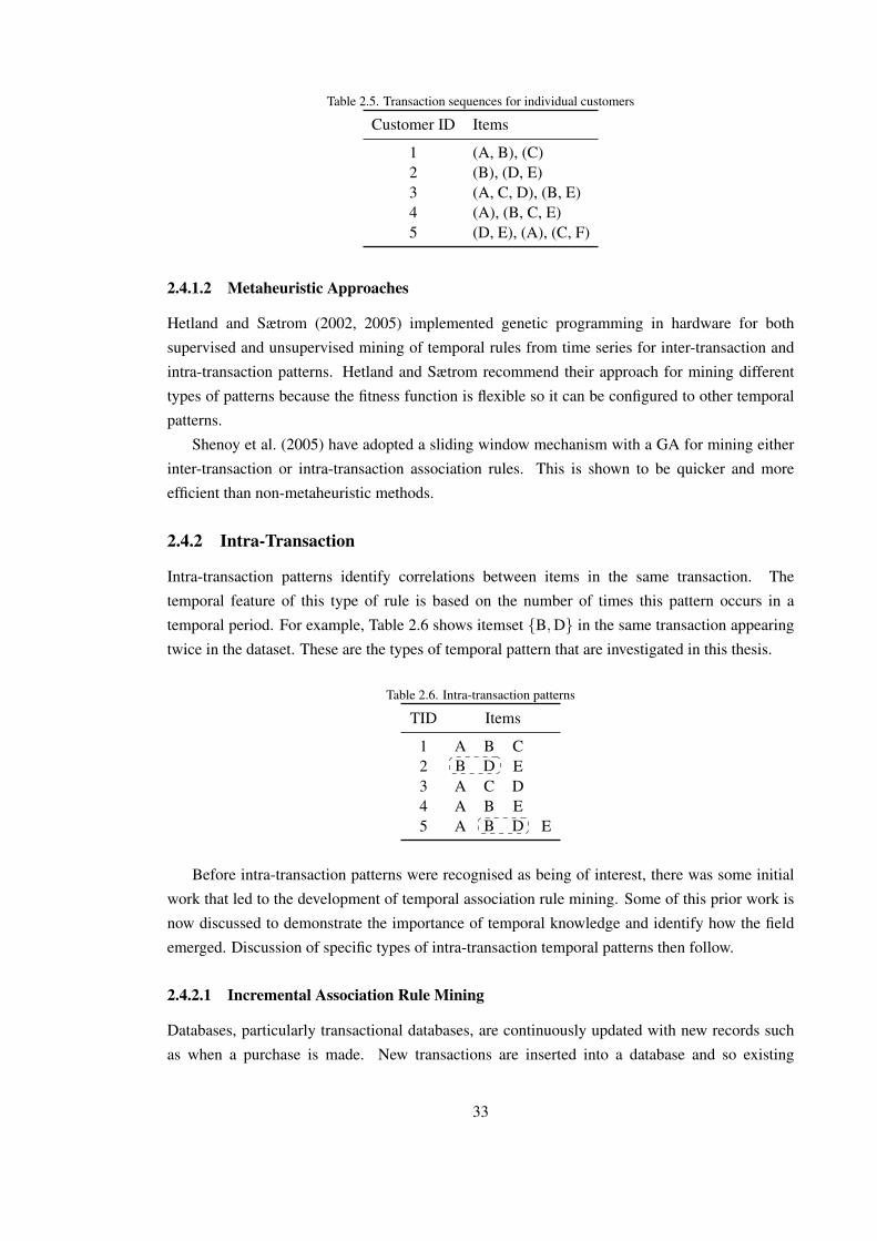
Table 2.5. Transaction sequences for individual customers
Customer ID Items
1 (A, B), (C)2 (B), (D, E)3 (A, C, D), (B, E)4 (A), (B, C, E)5 (D, E), (A), (C, F)
2.4.1.2 Metaheuristic Approaches
Hetland and Sætrom (2002, 2005) implemented genetic programming in hardware for both
supervised and unsupervised mining of temporal rules from time series for inter-transaction and
intra-transaction patterns. Hetland and Sætrom recommend their approach for mining different
types of patterns because the fitness function is flexible so it can be configured to other temporal
patterns.
Shenoy et al. (2005) have adopted a sliding window mechanism with a GA for mining either
inter-transaction or intra-transaction association rules. This is shown to be quicker and more
efficient than non-metaheuristic methods.
2.4.2 Intra-Transaction
Intra-transaction patterns identify correlations between items in the same transaction. The
temporal feature of this type of rule is based on the number of times this pattern occurs in a
temporal period. For example, Table 2.6 shows itemset {B,D} in the same transaction appearing
twice in the dataset. These are the types of temporal pattern that are investigated in this thesis.
Table 2.6. Intra-transaction patterns
TID Items
1 A B C2 B D E3 A C D4 A B E5 A B D E
Before intra-transaction patterns were recognised as being of interest, there was some initial
work that led to the development of temporal association rule mining. Some of this prior work is
now discussed to demonstrate the importance of temporal knowledge and identify how the field
emerged. Discussion of specific types of intra-transaction temporal patterns then follow.
2.4.2.1 Incremental Association Rule Mining
Databases, particularly transactional databases, are continuously updated with new records such
as when a purchase is made. New transactions are inserted into a database and so existing
33

association rules may be invalidated as new rules are introduced. It would be inefficient to
rerun the entire algorithm just to include the newly inserted transactions. So, the Fast Update
(FUP) algorithm (Cheung et al., 1996) was introduced to incrementally update existing association
rules. This is suitable for a non-trivial number of new transactions that are inserted frequently or
occasionally. For deletion, the FUP2 algorithm was introduced (Cheung et al., 1997). Incremental
updating has been extensively researched and is a method of maintenance that focuses only on
updating existing knowledge. Gharib et al. (2010) introduced an incremental mining algorithm
called Incremental Temporal Association Rules Mining (ITARM) for maintaining intra-transaction
temporal association rules. The Incremental Temporal Association Rule (ITAR) algorithm (Ng
et al., 2007) tackles the same task of maintaining temporal association rules that have numeric
attributes.
Prior to update algorithms, Agrawal and Psaila (1995) focused on analysing historical
association rules using active data mining. This method partitioned a database, mined association
rules from each partition and stored rules in a database of rules with the corresponding support
and confidence measures. The historical behaviour of association rules can be queried with
shape operators that define the temporal behaviour, such as a rule’s frequency going up, down,
or remaining stable. User defined triggers are based on rule conditions and provide a mechanism
for applying actions when triggers are activated. Although it does not mine or predict the changes
in association rules, it demonstrates an appreciation for changes and historical data.
Traditionally association rule mining assumes the entire dataset to be static meaning that the
rule is representative for the entire temporal period. The support value of a rule is calculated across
the entire dataset so resulting rules are assumed to be relevant for the entire period. However, in
real-world datasets this is not the case. Rules may occur over small temporal periods (e.g., music
festivals, religious events) or exhibit some recurring behaviour (e.g., weekends). Detecting and
adapting to changes is critical for businesses to be successful. Preventing lost opportunities can be
achieved with making timely decisions based on current and up-to-date information. Products or
services can be tailored with emerging knowledge of trends and requirements.
Dong and Li (1999) highlighted the importance of changing association rules for predictive
and descriptive data mining tasks. Au and Chan (2002) recognise the importance of changing
association rules, particularly so for predictive tasks such as classification. A dataset of flat prices
for the housing market was partitioned into years and then association rules were extracted. The
approach of Au and Chan constructed fuzzy rules from the association rules that represent the
changes in support and confidence through the years. These rules were used for associative
classification rule mining to predict flat prices. This demonstrates the widening importance of
association rules in dynamic environments and that is not limited solely to descriptive tasks.
2.4.2.2 Cyclic Association Rules
Cyclic association rules have support measures that change in temporal periods of a dataset (Ozden
et al., 1998). For example, these rules can analyse regular fluctuations of items. The dataset
is partitioned to a desired time granularity, e.g., day or week, and rules are induced from each
34
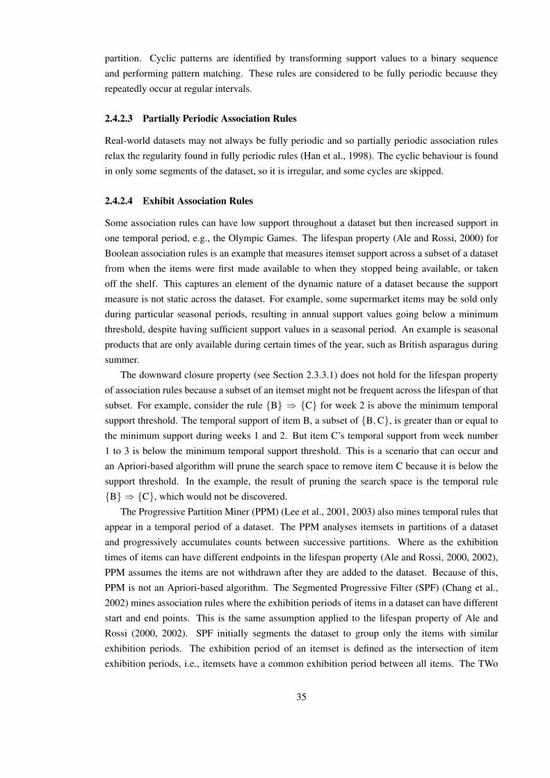
partition. Cyclic patterns are identified by transforming support values to a binary sequence
and performing pattern matching. These rules are considered to be fully periodic because they
repeatedly occur at regular intervals.
2.4.2.3 Partially Periodic Association Rules
Real-world datasets may not always be fully periodic and so partially periodic association rules
relax the regularity found in fully periodic rules (Han et al., 1998). The cyclic behaviour is found
in only some segments of the dataset, so it is irregular, and some cycles are skipped.
2.4.2.4 Exhibit Association Rules
Some association rules can have low support throughout a dataset but then increased support in
one temporal period, e.g., the Olympic Games. The lifespan property (Ale and Rossi, 2000) for
Boolean association rules is an example that measures itemset support across a subset of a dataset
from when the items were first made available to when they stopped being available, or taken
off the shelf. This captures an element of the dynamic nature of a dataset because the support
measure is not static across the dataset. For example, some supermarket items may be sold only
during particular seasonal periods, resulting in annual support values going below a minimum
threshold, despite having sufficient support values in a seasonal period. An example is seasonal
products that are only available during certain times of the year, such as British asparagus during
summer.
The downward closure property (see Section 2.3.3.1) does not hold for the lifespan property
of association rules because a subset of an itemset might not be frequent across the lifespan of that
subset. For example, consider the rule {B} ⇒ {C} for week 2 is above the minimum temporal
support threshold. The temporal support of item B, a subset of {B,C}, is greater than or equal to
the minimum support during weeks 1 and 2. But item C’s temporal support from week number
1 to 3 is below the minimum temporal support threshold. This is a scenario that can occur and
an Apriori-based algorithm will prune the search space to remove item C because it is below the
support threshold. In the example, the result of pruning the search space is the temporal rule
{B} ⇒ {C}, which would not be discovered.
The Progressive Partition Miner (PPM) (Lee et al., 2001, 2003) also mines temporal rules that
appear in a temporal period of a dataset. The PPM analyses itemsets in partitions of a dataset
and progressively accumulates counts between successive partitions. Where as the exhibition
times of items can have different endpoints in the lifespan property (Ale and Rossi, 2000, 2002),
PPM assumes the items are not withdrawn after they are added to the dataset. Because of this,
PPM is not an Apriori-based algorithm. The Segmented Progressive Filter (SPF) (Chang et al.,
2002) mines association rules where the exhibition periods of items in a dataset can have different
start and end points. This is the same assumption applied to the lifespan property of Ale and
Rossi (2000, 2002). SPF initially segments the dataset to group only the items with similar
exhibition periods. The exhibition period of an itemset is defined as the intersection of item
exhibition periods, i.e., itemsets have a common exhibition period between all items. The TWo
35

end AssocIation miNer (TWAIN) algorithm (Huang et al., 2007) is another exhibition rule mining
algorithm. TWAIN is able to discover more precise exhibition rules than PPM and SPF because
exhibition periods of items in an itemset can have different start and end points, i.e., the exhibition
period of each item does not necessarily overlap with the other items in an itemset.
2.4.2.5 Calendar-based Association Rules
Cyclic rules, partially periodic rules and exhibition rules use a single time granularity but
calendars express temporal patterns with multiple granularities, which is particularly suitable
for complicated temporal patterns. A calendric algebra has been created to formerly specify
complicated temporal patterns in Ramaswamy et al. (1998). The user specifies the calendar periods
for mining temporal association rules before the algorithm is executed. A calendar-based method
aims to be more applicable to real-world problems where periodicity has limited capabilities in
expressing change.
Calendar schemas (Li et al., 2001a, 2003) define the temporal intervals for discovering
association rules. The Apriori algorithm was modified to discover temporal patterns using
calendar-based schemas. Less prior knowledge is required than the calendric algebra of
Ramaswamy et al. (1998). A calendar pattern is defined from calendar units such as day, week
and month.
To enhance the general interpretability of expressing temporal patterns, fuzzy calendars were
introduced by Lee and Lee (2004) to allow rules to be described according to user requirements in
a calendar. For example, temporal patterns can be represented with linguistic terms such as every
summer and at the weekends.
Lee et al. (2008) and Lee (2008) use fuzzy calendars to express imprecise periodicities and
disturbances. The fuzzy periodic calendar has three types of components: crisp, fuzzy and cyclic.
Each calendar is required to have at least one cyclic component. The example provided by Lee
et al. (2008) states, “close to 15, June in every year” where “close to 15” is the fuzzy component,
“June” is the crisp component and “every year” is the cyclic component.
Verma et al. (2005) used tree data structures to enhance the execution time for mining calendar-
based association rules. The approach by Verma et al. utilised a Total-tree and a Partial-tree
(Coenen et al., 2001, 2004b,a).
2.4.2.6 Emerging Patterns
Emerging Patterns have an increase in support from one dataset to another. Early work constructed
models of datasets, which can be used for different mining tasks (e.g., classification, prediction),
and the difference between models is quantified by a deviation measure (Ganti et al., 1999). This
describes the amount of work required to transform one model to the other, for example, comparing
popular items sold in different stores. Although this does not model any explicit temporal aspect,
the same approach has also been used by Dong and Li (1999) to detect temporal patterns. A
framework proposed by Dong and Li (1999) measures the differences between two datasets for
36

the purpose of discovering emerging patterns. The difference in frequency of patterns, i.e., support,
between different datasets has been analysed. These approaches are restricted to two datasets.
2.4.2.7 Other types
This section of the literature review has focused on the temporal element of association rules being
expressed as either cyclic, partially periodic, exhibit period, calendar based or an emerging pattern.
All of which require prior knowledge of the type of temporal pattern sought to determine the most
suitable method. Li et al. (2006) created a framework to identify the type of temporal pattern
so specifying the type is not required before running the algorithm. The only prior knowledge
required is a time period of interest to the end-user.
Rare associations may occur infrequently (low support) but when it occurs it is simultaneous
with the specific data in high proportion (high confidence). Yun et al. (2003) have investigated
rare association rule mining. Association rules that are interesting because of rare or temporal
properties can be lost within association rule mining because measures can be below minimum
thresholds.
In real-world data there is often a temporal pattern present and there can be several types of
temporal pattern occurring simultaneously. This was first investigated by Zimbrao et al. (2002)
who incorporated lifespan into calendar based rules. Schluter and Conrad (2010) and Schluter
(2012) incorporated more than two elements of temporal association rules by using an efficient
approach with two tree structures: i) the extended partial support tree (EP Tree), and ii) the
extended target tree (ET Tree).
2.4.2.8 Metaheuristic Approaches
The intra-transaction temporal association rule mining algorithms that have been reviewed above
employ exhaustive search methods. The metaheuristics used for intra-transaction temporal
association rule mining are briefly reviewed here. Note that in Section 2.4.1.2 metaheuristic
approaches for inter-transaction temporal pattern were reviewed and Hetland and Sætrom (2002),
Hetland and Sætrom (2005) and Shenoy et al. (2005) are also relevant to this section because they
also mine intra-transaction patterns.
Martınez-Ballesteros et al. (2009, 2011) investigated intra-transaction patterns by using a GA
to find the intervals of quantitative attributes of association rules (reviewed in see Section 2.5.1)
from time series data. Their approach finds the temporal periods when specific quantitative
association rules occur.
2.4.3 Discussion
The main purpose of this section was to distinguish the different types of temporal pattern from
each other because the word temporal is ambiguous.
The different types of intra-transaction pattern were reviewed to clarify the exact type of
temporal patterns used in this thesis. Exhibit association rules are the type of temporal pattern
37

that are sought. It will be discussed in Section 7.3 that future work could be directed towards other
types of temporal pattern than those reviewed here.
Metaheuristics have been applied to both inter-transaction and intra-transaction rule mining.
The main benefits of metaheuristics for temporal association rule mining are the flexibility in
defining the type of pattern and the ability to find rules that are specific to certain temporal periods.
The review has also noted how tree data structures have been used for intra-transaction
temporal association rule mining.
2.5 Fuzzy Association Rule Mining
This section focuses on the other extension to classical association rule mining, the fuzzy feature.
Research using classical set theory in quantitative association rule mining and utility association
rule mining is reviewed first. Fuzzy association rule mining is then reviewed. Each subsection
reviews the use of exhaustive search methods as well as metaheuristics.
2.5.1 Quantitative Association Rule Mining
Association rule mining finds correlations among items in Boolean data. Quantitative association
rule mining extends this by discovering correlations in quantitative attributes. Research into this
area preceded fuzzy association rule mining.
Srikant and Agrawal (1996) introduced mining quantitative and categorical association rules.
Quantitative items were uniformly discretised into crisp sets and a descriptive label was mapped to
each set. Categories and crisp sets of quantities are handled as items so that the Apriori algorithm
can be applied. For example, a gender attribute has two values, so instead of one item for both
male and female there is one item for male and one item for female. The inclusion of quantities
makes this a problem of discovering correlations between the intervals of items, rather than just
the items. Partitioning attributes is considered to be another stage in a KDD methodology to that
of data mining (step 6 of the KDD Process in Section 2.3.1). Srikant and Agrawal recognised
that partitioning attributes into intervals causes a loss of information. They introduced the partial
completeness measure to quantify the information loss, which considered minimum support, and
used the measure to determine the number of partitions. The number of partitions was chosen to
satisfy the level of partial completeness. The partitions were defined using equal width partitioning
by splitting the range of an attribute’s value into equal width intervals.
The Birch clustering algorithm was used by Miller and Yang (1997) for equal frequency
partitioning, which places an equal number of values into an interval. This is more suitable for
data that can have transactions that are skewed within individual partitions. They also proposed a
distance-based association rule mining process for improving the semantics of the intervals. These
methods of equal width and equal frequency partitioning are common methods of discretisation
for unsupervised learning (Yang et al., 2010).
Statistical inference theory was used by Aumann and Lindell (2003) for quantitative
association rule mining. A new definition was introduced that has the form
38

{population-subset} ⇒ {extraordinary-behavior}
The population-subset describes a subset of the population and the extraordinary-behavior is a
description of a behaviour particular to that subset. For example, ‘Sex = female⇒ mean wage =
$7.90 p/hr’ (Aumann and Lindell, 2003).
Further to the discretisation and statistical methods, there are many methods that have used
evolutionary computation (del Jesus et al., 2011). Mata et al. (2001) have used a GA for
quantitative association rule mining. Mata et al. (2002) used a GA for quantitative itemset mining.
Both methods search for attribute intervals specific to each rule and use IRL. Once a rule/itemset
is discovered, the corresponding records of the database that match that rule/itemset are penalised.
The fitness function then penalises individuals according to the number of records that the
individual has covered in previous iterations. Another example of evolutionary computation
applied to quantitative association rule mining is Differential Evolution (Alatas et al., 2008).
Association rule mining can be applied to different types of dataset such as transaction datasets
and relational datasets. The GAs methods reviewed here are applied to relational datasets so they
have fixed length chromosomes to match the number of attributes in the dataset.
Alcala-Fdez et al. (2010) have compared several approaches that use GAs for quantitative
association rule mining. Alcala-Fdez et al. demonstrated good confidence values, linear scalability
with respect to time and a reduced set of rules where the total number is restricted by the number
of iterations in IRL.
A disadvantage of quantitative association rule mining is the crisp boundaries of discretised
values that potentially hide rules and lose information (Mata et al., 2002). The next section
presents a closely related area, utility association rule mining, and the section following that
introduces the use of fuzzy logic to overcome this problem.
2.5.2 Utility Association Rule Mining
The numeric attribute of an item can represent more than the quantity of an item, it can represent
some notion of the item’s utility. Utility association rule mining discovers patterns that can have
high importance but low support values. For example, high value products may be sold less
frequently, e.g., Champagne. This type of problem was first recognised by Cai et al. (1998) who
assigned weights to items in a rule (see Section 2.3.5.2). Barber and Hamilton (2003) use the share
measure for mining quantitative itemsets where the transaction is attributed with a total quantity
of items sold or a total profit. Yao et al. (2004) provided a clear definition of two types of utilities
that explains the difference well: transaction utility and external utility. The transaction utility is
defined by information present in the transaction, such as the quantities of items. The external
utility is defined by information from other sources that are outside of the transaction, such as
profit, or nutritional information. Muyeba et al. (2009) and Khan et al. (2011) used composite
association rules with nutritional information because each item contains multiple attributes such
as protein and fibre, to mention a few.
The temporal aspect of utility association rule mining has been investigated. This is of interest
39

to this thesis because the temporal feature is combined with a numeric feature. Lin et al. (2010)
handle the incremental update problem (see Section 2.4.2.1) where new transactions are added to
the dataset. An HUP tree is an extension of the FP-tree used for updating with new transactions
from the dataset. Tseng et al. (2006) and Chu et al. (2008) investigated temporal patterns that occur
in data streams by analysing patterns in a current time window. Maragatham and Lakshmi (2010)
have explored temporal patterns in utility mining by modelling the utility of items as dynamic. A
dataset is partitioned according to a temporal unit, such as day, week and month. Specific utilities
of items are assigned to each partition so the utilities are different in each temporal period.
2.5.3 Fuzzy Association Rule Mining
Classical set theory has been applied to quantitative association rule mining. The review is now
extended to include the use of fuzzy set theory for fuzzy association rule mining. Methods
that search for fuzzy association rules using exhaustive search methods are reviewed here.
Metaheuristic approaches for fuzzy association rule mining then follow.
Yager (1982) suggested fuzzy sets for summarising data with linguistic terms in data mining.
This provided a less terse summarisation than typical average and sum measures that can help
to understand the data. Maeda et al. (1995) extend this to rule induction by introducing the idea
that fuzzy sets can enhance the interpretability and improve robustness to noise for rule induction.
Fuzzy association rules were introduced to express quantitative attributes with linguistic labels
in a way that is more natural to human reasoning. Chan and Au (1997) proposed F-APACS for
mining fuzzy association rules and this improved the representation of quantitative attributes with
inaccuracies in physical measurements. Rather than use a subjective measure of user-defined
thresholds, such as minimum support, Chan and Au used an objective measure called adjusted-
difference. The linguistic terms and membership functions were elicited from an expert. This
approach followed the following two-stage procedure:
1. Define the linguistic terms and membership functions.
2. Mine fuzzy association rules using the defined linguistic terms and membership functions.
Fuzzy association rules also deal with unnatural boundaries of crisp intervals (Kuok et al.,
1998). The crisp boundary problem (also referred to as the sharp boundary problem) exists because
an attribute may occur near a boundary of a crisp interval but has the same set membership as
if it occurred in the middle. Fuzzy sets overcome this because they provide variability in set
membership near the boundaries of fuzzy sets. Kuok et al. also elicited linguistic terms and
membership functions from experts. Kuok et al. used product implication and divided the total
support (referred to as significance in their paper) by the total number of records.
Various algorithms that perform Boolean association rule mining have been adapted for fuzzy
association rule mining. Fuzzy Frequent Pattern-growth (FFP-growth) (Wang et al., 2010) is an
algorithm based on FP-growth (see Section 2.3.3.2). Hong et al. (1999) introduced the Fuzzy
Transaction Data-mining Algorithm (FTDA). Hong et al. later improved upon this work with
FuzzyApriori in Hong et al. (2001), which is an adaptation of Apriori. The fuzzy support measure
40

used minimum implication. Fuzzy Apriori-T (Khan et al., 2008) is based on the T-tree structure
(Coenen et al., 2004a) that enhances the efficiency of the search process. Muyeba et al. (2009)
adapted the Apriori algorithm to handle fuzzy values and also included a tree structure. A common
feature of these algorithms adapted for fuzzy association rule mining is the measure of fuzzy
support, which is Boolean support adapted to handle fuzzy sets.
Chan and Au (1997) and Kuok et al. (1998) used domain experts to define linguistic terms
and membership functions for fuzzy association rule mining. To automatically define the
membership function parameters specifically for association rule mining there has been clustering
(Fu et al., 1998; Kaya et al., 2002), GA-based clustering (Kaya and Alhajj, 2003, 2005) and GAs
(Hong et al., 2008). Hong et al. (2008) used a divide and conquer strategy with a GA to learn
membership functions before running FuzzyApriori. The divide and conquer strategy had multiple
populations and each population was assigned to learn the membership function of one item.
The evolutionary process only selects and recombines chromosomes from the same populations.
These methods serve the purpose of automatically defining the membership functions, which is
considered learning in the taxonomy of how GFSs are applied (discussed in Section 2.2.3). They
have also been used to tune the membership functions.
Chen et al. (2007) mine fuzzy association rules with multiple minimum support thresholds.
They initially cluster items with similar characteristics and assign “reasonable membership
functions” (Chen et al., 2007, p.1734) to initialise the population. This is considered to
automatically identify the membership functions and then tune the parameters with a GA.
Alcala-Fdez et al. (2009a) learnt the context of membership functions by using the 2-tuple
linguistic representation (Herrera and Martınez, 2000). The linguistic labels and membership
functions were defined first from a domain expert so the GA is considered to be tuning the
membership functions parameters and learning the contexts of those membership functions.
Alcala-Fdez et al. also demonstrated how CHC can outperform other methods such as the divide
and conquer strategy of Hong et al. (2008).
The work reviewed so far in this section has followed the two-stage procedure, discussed
earlier in this section, where the linguistic labels and membership functions are defined first
before mining fuzzy association rules. The review of quantitative association rules in Section 2.5.1
revealed how a GA can be used to simultaneously evolve the crisp intervals and association rules
(i.e., Mata et al. (2001, 2002)). The approach of simultaneously evolving both components has
been applied to only one fuzzy association rule mining algorithm. Kaya (2006) investigated a
similar approach with MOEA for simultaneously learning membership function parameters and
fuzzy association rules. The reason for simultaneously learning both components is unclear.
However, in this thesis there is a well-justified reason of discovering rules that are otherwise lost
with a traditional approach. This will be discussed more in Chapter 4.
Despite fuzzy association rule mining being a popular research field, which is evident from
the many reviews and surveys, e.g., Hong and Lee (2008), Chen et al. (2009) and del Jesus
et al. (2011), there has been some debate over the suitability of using fuzzy sets in association
rule mining. The use of fuzzy association rule mining over crisp association rule mining should
be justifiable in terms of the crisp boundary problem and the interpretability of knowledge
41
represented as linguistic terms. Verlinde et al. (2005) compared quantitative association rules with
fuzzy association rules using a data-driven approach of determining the membership functions
by clustering the data. They concluded that there is no significant difference between fuzzy
rule mining and quantitative rule mining. The discussion on their analysis was welcomed by
Hullermeier and Yi (2007) who extended the experimental analysis. Hullermeier and Yi claim
their results are not proof of the usefulness of fuzzy association rules. But, they conclude that
using different partitioning methods, focusing on more complex rules (with antecedents greater
than one), and analysing the best rules can produce very different results between both fuzzy and
crisp association rule mining.
Subgroup discovery is very similar to fuzzy association rule mining. Subgroup discovery is
a task of knowledge discovery introduced by Klosgen (1996) and Wrobel (1997) and defined by
(Lavrac, 1998, p.19) as: “Given a population of individuals and a property of those individuals
we are interested in, find population subgroups that are statistically ‘most interesting’, i.e., are as
large as possible and have the most unusual statistical characteristics with respect to the property
of interest”. Subgroup discovery is a method of supervised inductive learning that draws concepts
from both descriptive induction and predictive induction. Subgroup discovery is considered to be
descriptive induction because the aim is to locate subgroups with interesting patterns through a
process of search and discovery. Subgroup discovery is also considered to be predictive induction
because of the subgroup description, which takes the form Cond⇒ Class. Carmona et al. (2010)
have applied nondominated sorting genetic algorithm II (NSGA-II) to subgroup discovery with
Non-dominated Multiobjective Evolutionary algorithm for Extracting Fuzzy rules in Subgroup
Discovery (NMEEF-SD). NSGA-II is a multi-objective evolutionary algorithm created by Deb
et al. (2002). Subgroup discovery looks for unusualness of a class and associative classification
rules do not (see Section 2.3.5.3).
Utility association rules have been extended with fuzzy logic to describe the quantities of
utilities with words. The approaches by Muyeba et al. (2009) and Khan et al. (2011) for composite
association rules are examples that also use fuzzy association rules.
The origins of Boolean association rule mining come from market basket analysis (Agrawal
et al., 1993). Applications of fuzzy association rule mining have also followed this, for example,
the following have all used transaction market basket datasets: Au and Chan (2002); Kaya and
Alhajj (2004); Xie (2005); Chen et al. (2006, 2007); Hong et al. (2008); Chen et al. (2009). Other
applications on transaction datasets include: network intrusion detection (Su et al., 2011), web
mining (Wong et al., 2001; Arotaritei and Mitra, 2004), bioinformatics (Lopez et al., 2008) to
mention a few. Applications on relational datasets are also popular with fuzzy association rule
mining, such as: population surveys (Delgado et al., 2003; Alhajj and Kaya, 2008; Alcala-Fdez
et al., 2009a) and marketing (Orriols-Puig et al., 2009) to mention a few.
2.5.4 Discussion
The literature has shown how the first type of association rule mining with numeric attributes
discretised the values into crisp sets. This was later improved by using fuzzy sets instead of
42

crisp sets. Historically, modelling of systems focused on accuracy first, before soft computing
techniques were available such as fuzzy logic (Cordon, 2011). For association rule mining, the
same historical approach is evident from the literature review. This shows the application of crisp
sets for interval-based association rules before fuzzy sets and linguistic labels were applied to the
problem. GAs have been applied to define the crisp sets for quantitative association rule mining
and the fuzzy sets for fuzzy association rule mining. A closely related area is utility association
rule mining.
For fuzzy association rule mining there have been a variety of methods for learning and
tuning the fuzzy sets of linguistic terms. Literature on this subject has demonstrated how
fuzzy association rule mining involves either: learning membership functions first before mining
rules; simultaneously learning both membership functions and rules; or, learning the membership
functions and then tuning the membership function parameters before mining rules. Methods of
learning rules include both exhaustive search processes and metaheuristic methods, specifically
GAs.
2.6 Temporal Fuzzy Association Rule Mining
This thesis explores a previously unrecognised problem of how some fuzzy association rules can
be lost because the contextual meaning of linguistic terms changes in temporal periods of the
dataset. This section highlights existing research that is close to this thesis but differs in some way.
The review now contextualises previous research within the scope of this previously unrecognised
problem. Academic and news articles from industry were both reviewed in this section.
2.6.1 Academia
Early work on temporal fuzzy association rule mining explored how the quantitative values can
change over time. For example, the prices/sales of items rising over a week/month (Wang et al.,
2001). The temporal aspect of Wang et al. (2001) focused on the quantitative values changing
and the temporal feature is described as “evolving numerical attributes”. This is similar to the
incremental approach of maintaining quantitative association rules in Ng et al. (2007).
Martınez-Ballesteros et al. (2011) focused on intra-transaction temporal patterns found in
quantitative association rules. Multi-dimensional time series data was used and crisp partitions
of attribute intervals were specific to each rule. The research of Martınez-Ballesteros et al. (2011)
differs from this thesis because crisp intervals of attributes and multi-variate time series data are
used.
Balasubramanian and Duraiswamy (2009) and Balasubramanian et al. (2010) investigated
intra-transaction temporal association rule mining and also fuzzy association rule mining.
Investigations on the two types of association rule mining were reported in each individual paper
but the types of association rule mining were not combined.
Tseng et al. (2006) mined intra-transaction temporal patterns of utility itemsets. Tseng et al.
(2006) focused on data streams where the patterns discovered were relevant in a current time
43
window. Maragatham and Lakshmi (2010) have focused on the same problem of discovering
intra-transaction temporal patterns in utility mining. They partition a dataset into temporal units,
such as day, week and month. Specific utilities of items are assigned to each partition so the
utilities are different from one temporal period to the next, which means that the temporal aspect
of the utilities is more dynamic than the approach in Tseng et al. (2006). Pillai et al. (2010)
investigated mining intra-transactional temporal patterns for utility itemsets. The aim of Pillai et al.
(2010) was to find rare itemsets that have high utility such as profit. The temporal behaviour of
utility values was modelled such that the cyclic, semi-cyclic or non-cyclic behaviour was recorded.
Yun and Ryu (2011) recognise that changes in weights of items, in noisy environments, can
cause large changes in weighted association rules. One aspect of Yun and Ryu (2011) is similar to
this because this thesis also focuses on a change that may be present in the data, however, Yun and
Ryu (2011) use crisp weight values. The approximate factor in Yun and Ryu allows for variability
in the support of a weighted association rule.
The works surveyed here all use crisp values of partitions of the quantitative/weight/utility
attributes. Hong et al. (2002), Huang and Kao (2005) and Hong et al. (2006) used fuzzy logic to
partition quantitative attributes for inter-transactional temporal patterns, i.e., sequence rules.
Shenghan et al. (2011) have used the 2-tuple linguistic representation in a temporal context.
The lateral displacement was used to model an event occurring in the past (α = −0.5), present
(α = 0) or future (α = 0.5). A fuzzy model was developed for evaluating risk and when risk
occurs.
Fuzzy Apriori Rare Itemset Mining (FARIM) discovers fuzzy association rules whose
frequency in a dataset is referred to as rare (Weng, 2011). Weng apply FARIM to educational data
to discover patterns that can identify students who have different scores to the average student that
could suggest there is a problem. The problem proposed by Weng (2011) is similar to the problem
stated in this thesis because fuzzy association rules can be lost because of their frequency in a
dataset. In the case of Weng (2011), the lose is only caused by a pattern’s rareness. But, in this
thesis the problem relates to how the fuzzy sets are defined.
2.6.2 Industry
The discussion of business activities can be commercially sensitive for businesses and there
is much less literature available from industry. Activities of businesses are important for
understanding the wider significance of the previously unrecognised problem presented in this
thesis.
An article in FORTUNE magazine (Leonard, 2005) reports on how temporal patterns in
supermarket datasets occurred during Hurricane Katrina. The sale of items, such as water and
flashlights (torches in British English), are associated with Strawberry Pop-Tarts (a pre-baked
product heated up in a toaster that consists of two layers of pastry with a sweet filling from the
USA). This appears to be an odd association that may be present because the items co-occur
in transactions by chance. However, in the context of Hurricane Katrina, a causality that can
be speculated: Pop-Tarts are high-energy comfort food that may be considered to be of equal
44
usefulness and importance as emergency items, such as water and flashlights. As suggested in
Yoo and Shekhar (2009), this knowledge can be used to improve the operation of supply chains
and improve the visibility of items during key times.
Saleh and Masseglia (2010) report on the increase in sales of specific items during the Super
Bowl (a championship game for American football in the USA). There were an increase in sales
of guacamole, chips (crisps in British English) and antacid during the period of the Super Bowl.
This does not state that there were associations between the items in a transaction (intra) or
across multiple transactions (inter). However, it exemplifies how a scheduled event can change
the context for quantities of items sold.
An article in The New York Times Magazine (Duhigg, 2012) reports on how quantitative
and temporal patterns in data can be used to identify and develop profiles of potential customers.
Knowledge of these profiles allows companies to target advertising more effectively.
Although fuzzy logic is not stated as having been used in the literature from industry, the
literature does refer to quantitative data that can be represented with fuzzy sets.
2.6.3 Discussion
The review of the literature has focused on previous research and applications that explore the
composition of temporal association rule mining and fuzzy/quantitative association rule mining.
The review has not identified previous work that either recognises or tackles the problem defined
in this thesis (Section 1.1). Some of the literature reviewed is similar to the problem proposed
in this thesis. However, no literature has been discovered that tackles the same problem as this
thesis. So, this supports the identification of the previously unrecognised problem. Furthermore,
the importance of the problem is evident in industry from the literature in internationally renowned
magazines, such as FORTUNE magazine and The New York Times Magazine.
There are algorithms that incorporate both the fuzzy and temporal elements of association
rules. However, the temporal element is for inter-transactional temporal patterns, i.e., sequence
rules, and not intra-transactional temporal patterns such as exhibition periods. The algorithms
reviewed here are unsuitable for evaluating the research hypothesis, because the temporal pattern
is different to that sought in this thesis, so they are not used in this thesis.
2.7 Web Mining
The real-world dataset used in this thesis is a Web log dataset. Literature from this domain is
reviewed here to provide background and state-of-the-art knowledge.
Etzioni (1996) defined Web mining as “the use of data mining techniques to automatically
discover and extract information from World Wide Web documents and services”. Three
categories of Web mining were later defined by Madria et al. (1999) and Borges and Levene (2000)
as: i) Web content mining, ii) Web structure mining, and iii) Web usage mining. A survey of the
categories has been conducted by Srivastava et al. (2000) and an explanation of each category is
now given. The terminology and definitions for discussing the Web were defined by the World
45

Wide Web Consortium (1999) and are used throughout this thesis.
Web content mining is the task of discovering useful knowledge from the content/data of
Web sites, such as text, images and videos. Cooley et al. (1997b) have further categorised the
purpose of Web content mining based on the perspectives stated by Srivastava et al. (2000) as
either information retrieval or database. The information retrieval perspective attempts to find
or retrieve information from large sources. Web content mining, from the database perspective,
attempts to model data to allow further analysis with database queries.
Web structure mining attempts to discover knowledge about the underlying structures that link
Web pages (Chakrabarti et al., 1999). Hyperlinks in Web pages can be used to identify Web sites
that are authoritative on a subject and model the topology of Web sites for comparison with other
Web sites.
Web usage mining attempts to discover patterns of user behaviours that are recorded in the logs
of Web servers as users browse and navigate Web sites (Cooley et al., 1997b). This is the Web
mining category of the real-world application of this thesis. Web usage mining uses secondary
Web data that is generated from the users, whilst Web content mining and Web structure mining
use primary data (Srivastava et al., 2000). Web usage data can include Web server access logs,
proxy logs, user sessions, cookies, to mention a few.
Srivastava et al. (2000) categorised the application of Web usage mining is either personalised
for learning user profiles, or unpersonalised for user navigation patterns. The knowledge
discovered from Web usage mining can be used in many ways, for example, redesigning parts
of a Web site so they are more effective and supporting business decisions. Association rules,
and sequential rules, can represent user navigation patterns on the Web. Facca and Lanzi (2005)
reviewed the methods of Web usage mining and their application.
2.7.1 Data Cleaning and Preprocessing
Data cleaning and preprocessing is an important stage of the KDD Process (see Section 2.3.1).
Data cleaning for Web usage mining involves removing records in a Web log that are not important
(Cooley et al., 1997b). Typically this is accomplished by removing records with uniform resource
locator (URL) requests that have suffixes, such as jpg.
User identification is a problem for two reasons (Cooley et al., 1997b; Cooley, 1999). First,
when a proxy server is present, the machine name of a request may refer to the proxy server that
can have multiple users behind it. Proxy servers may be present in Internet Service Providers and
companies/organisations. Also, a proxy server may provide local proxy caching of Web pages to
one or more users. When a cache is used the content is provided by the cache system and not
the Web site. The second problem of user identification is again related to cache, but at the PC
where a user is viewing the Web site. For example, when a user clicks back the Web page is
often loaded from cache and not the Web site. There are numerous solutions to the problem of
user identification and some of these are mentioned here. Pirolli et al. (1996) used a web site’s
topology of hyperlinks/structure to provide knowledge of which Web pages were traversable from
a current Web page in order to ascertain users from the same incoming request. Pitkow (1997)
46

suggest using members who have registered on a Web site or Internet protocols, such as the Ident
Protocol and the Finger protocol, to identify a single user at the other end of a request. Elo-Dean
(1997) used cookies to identify users accessing the 1996 Olympics Web site.
Transaction identification is the problem of breaking down a user session into transactions
(Cooley et al., 1997a). This is also referred to as sessionisation. A user session is a sequence of
URL requests from the same user and the transaction identification problem refers to creating a
subset of sequences of URL requests. For example, a session may contain a request at 9am and
then a request at 3pm in the same day. It cannot be assumed that the user has viewed the Web
page for 6 hours because they may have minimised the Web browser or walked away from the
PC. Also, the problems behind user identification mean that it cannot be assumed that this request
came from the same user.
Unlike market basket datasets, Web log datasets comprise many URL requests that are not
naturally clustered into transactions. There are three methods for transaction identification:
reference length, time window and maximal forward reference. These are now explained.
Reference length transaction identification uses the concept that a Web page can be categorised
as either navigation or content (Cooley et al., 1997a). A navigation reference is a Web page that
a user traverses in order to find the information they require on a content reference Web page.
Cooley et al. (1997a) proposed a method of analysing the Web page view times and asserting a
cutoff time to categorise Web pages as either navigation or content references. The usefulness
of this depends on the goal of applying Web usage mining to a specific problem, i.e., to find
navigation and content patterns or content-only patterns.
Time window transaction identification is a time-oriented heuristic where by the duration of
a session must not exceed a threshold (Cooley et al., 1997a). The time threshold is a crucial
parameter in time window transaction identification. This is also a method of user identification,
which was discussed before transaction identification.
Maximal forward reference transaction identification creates a new transaction when a user
makes a backward reference (i.e., revisits a previous page in the current transaction) and then a
forward reference to a new Web page (Chen et al., 1996). A new transaction is created when a
forward reference is made. For example, the traversal path of a user {A,B,C,D,C,E,G} would
be split into transactions {ABCD,ABEG}, which are known as the maximal forward references.
2.7.2 Computational Intelligence in Web Usage Mining
CI is particularly useful in Web usage mining. Fuzzy logic is suitable for handling uncertainties
and the human interpretation of notions such as a short or long time spent viewing a Web page.
Evolutionary computation is suitable for searching large and complex search spaces that are found
in Web usage mining. Artificial neural networks are omitted because this is beyond the scope of
this thesis. The application of CI in Web usage mining is reviewed.
47
2.7.2.1 Fuzzy Logic
Fuzzy logic has been applied to the three categories of Web mining defined in Section 2.7
(Nikravesh et al., 2002; Arotaritei and Mitra, 2004). The review of fuzzy logic focuses on Web
usage mining.
Wong et al. (2001) mined fuzzy association rules from Web log data where the fuzzy attribute
was the time spent on a Web page. The number of fuzzy association rules were reduced after
the mining process by merging similar rules. The real-world dataset used by Wong et al. was
augmented with random values for the time spent on a Web page. The fuzzy rules were integrated
with a case based reasoning system that was demonstrated to have good prediction accuracy.
Martınez et al. (2003) regarded the support and confidence measures of Boolean association
rules as fuzzy variables. Martınez et al. created a FRBS applied to the Apriori algorithm, to
enhance the level of intuitiveness of defining the minimum thresholds.
Fuzzy association rule mining has been used for a recommender system to make personalised
learning recommendations in an e-learning environment (Jie, 2004). Fuzzy associations are
generated that correlate a student’s requirements to a list of learning materials.
As previously discussed in Section 2.7, Hong et al. (2002) mined inter-transaction temporal
fuzzy association rules, i.e., sequences. The application of the work was in Web usage mining
where the sequence of Web pages visited was analysed.
2.7.2.2 Evolutionary Computation
Anandarajan (2002) learnt the weights of an artificial neural network, with a GA, for classifying
employee profiles according to employee Web usage behaviour. Nasraoui and Krishnapuram
(2002) use a GA-based clustering algorithm to identify associations amongst URLs. Nasraoui
and Rojas (2003) used a GA to mine Web user profiles from dynamic Web log data. The benefit
of the approach by Nasraoui and Rojas (2003) is the capability of learning Web user profiles that
are dynamic and continuously changing. Streaming data is continuously passed to the algorithm
rather than reading an entire dataset in one operation that may not fit in memory. Tug et al. (2006)
used a GA for mining inter-transaction temporal fuzzy association rules, i.e., sequences.
2.7.2.3 Genetic Fuzzy Systems
The use of hybrid CI methods has been less common in the literature. A theme amongst the
use of GFSs for Web usage mining is the data mining task, subgroup discovery (discussed in
Section 2.5.3). Romero et al. (2009) mine fuzzy rules for subgroup discovery for an e-learning
system called Moodle. Carmona et al. (2012) applied NMEEF-SD to subgroup discovery for a
commercial Web site.
2.7.3 Discussion
This review of literature has shown that Web mining has been applied in three key areas. The
real-world dataset used in this thesis is a Web log dataset for Web usage mining. Methods for
48

cleaning and preprocessing the data have been identified that will be discussed further when they
are applied in Section 3.2. This review of CI methods in Web usage mining has focused on the CI
methods used in this thesis.
49

Chapter 3
Datasets
Understanding the decisions made in creating a solution for the hypothesised problem requires
understanding of the datasets. So the type of dataset and its features are clarified here before
presenting the GA-based framework in the next chapter. Both the synthetic and real-world datasets
required modifications to how the dataset is either generated or preprocessed. Two datasets were
used to demonstrate the ability of the proposed solution to generalise to synthetic and real-world
datasets as well as different domains.
3.1 Synthetic
A synthetic dataset generator was used for controlled experiments and analysis of datasets with
different dimensions. There are synthetic dataset generators for association rule mining that were
designed for market basket analysis: i) the IBM Quest synthetic dataset generator (Sourceforge,
2010), ii) ARMiner (Cristofor, 2000), and iii) ARtool (Cristofor, 2001). The IBM Quest synthetic
dataset generator is used in this thesis and can be considered as a benchmark because of its use in
many previous research projects on Boolean association rule mining, such as the seminal Apriori
algorithm, FP-growth and Eclat (see Section 2.3.3 for a description of each).
The IBM Quest synthetic dataset generator is suitable for mining Boolean association rules
and was created by Agrawal and Srikant (1994) to accompany the Apriori algorithm. The dataset
generator produces a market basket dataset that consists of transactions containing items. The
dataset generator is a computer program that produces datasets from input arguments. The input
parameters of the IBM Quest synthetic dataset generator are listed in Table 3.1 with the default
values. A random seed is also supplied to the dataset generator.
Table 3.1. Parameters of the IBM Quest synthetic dataset generator
Notation Default Description
|D| 1000000 Number of transactions|T | 10 Average size of the transactions|I| 4 Average size of the maximal potentially large itemsets|L| 10000 Number of maximal potentially large itemsetsN 100000 Number of items
50

An overview of the algorithm for the IBM Quest synthetic dataset generator is provided below
and further details are available in Agrawal and Srikant (1994).
1. A set of maximal potentially large itemsets τ is set to a size of |L|. The maximal
potentially large itemsets in τ are the patterns that transactions will be constructed from.
They are maximal frequent itemsets that can potentially create patterns in transactions (see
Section 2.3.3.1 for a definition of maximal frequent itemset). For example, a maximal
frequent itemset can represent a bicycle, helmet and gloves, from which some customers
may purchase only a bicycle and helmet. Thus, multiple patterns can be generated from the
same maximal frequent itemset. To generate the first maximal potentially large itemset in
τ , its size is generated from a Poisson distribution with mean λ = |I|. The items are then
randomly generated from N items for the first maximal potentially large itemset. Remaining
members of set τ are randomly generated from the previously generated itemset (with a
specified level of correlation) to model the phenomenon of common items in large itemsets.
2. The size of each transaction (i.e., number of items in each transaction) is selected from a
Poisson distribution with mean λ = |T |.
3. For each transaction, of the total number |D|, a series of maximal potentially large itemsets
are randomly chosen from τ and assigned to a transaction. At this stage, no items are in the
transaction, there is only a series of itemsets associated with the transaction.
4. Itemsets are then selected and placed into the transaction from the series of maximal
potentially large itemsets that were assigned to a transaction. Each maximal potentially
large itemset in τ is assigned a weight that determines the probability of being selected. If
the selected itemset does not fit in the transaction then, in 50% of cases it is added regardless,
and in the other 50% of cases it is added to the next transaction.
The dataset generator defined in Agrawal and Srikant (1994) does not generate transactions
with quantitative attributes. So the dataset generator was extended in this thesis to include
quantitative attributes. The extension is a similar approach to Liu et al. (2005) and Tsai and
Chen (2006). In the last stage of the algorithm for creating datasets (stage 4 in the overview for the
dataset generation algorithm of Agrawal and Srikant (1994)) the quantities of items were randomly
generated from a uniform distribution and assigned to each item in a transaction. Table 3.2 shows
a sample dataset generated from modifications to the IBM Quest synthetic dataset generator. Note
that the number of items in each transaction varies and each item is not stored in a separate column
(i.e., not a table data with fixed columns).
The dataset generator has the option of producing inter-transaction temporal patterns (i.e.,
sequences), but there is no option for intra-transaction temporal patterns. Although there are
intra-transaction temporal dataset generators, they do not include quantitative attributes and they
are not widely used in the research community. These include: tBasket (Li et al., 2001b), TARtool
(Omari et al., 2008) and TARGEN (Schluter and Conrad, 2009).
51

Table 3.2. Sample dataset from IBM Quest synthetic dataset generator (item IDs are replaced with descriptive namesfor illustrative purposes)
TID Items
1 {bread(12), pizza(2), beer(1)}2 {eggs(6), milk(1)}3 {eggs(2), pizza(4)}4 {bread(4), cheese(18)}5 {cheese(2), pizza(5), beer(15)}6 {pizza(5), beer(15), milk(18)}7 {eggs(18), cheese(3)}8 {bread(3), eggs(12), cheese(1)}9 {pizza(1), cheese(9)}10 {bread(1), pizza(11)}
The IBM Quest synthetic dataset generator has a set of maximal potentially large itemsets that
all transactions are created from (stage 1 in the overview for the dataset generation algorithm
of Agrawal and Srikant (1994)). This stage ensures that the same patterns occur in multiple
transactions of the dataset. This feature makes the dataset generator suitable for intra-transaction
temporal association rule mining because there are common patterns (i.e., rules) amongst
transactions. The dataset generator produces a TID for each transaction and not a timestamp. The
assumption is made that transactions occur at uniform periods of time represented by a TID. The
IBM Quest synthetic dataset generator has been applied for intra-transaction temporal association
rule mining with cyclic patterns (Ozden et al., 1998), exhibition periods (Chang et al., 2002) and
calendars (Li et al., 2003).
3.2 Real-World
Synthetic datasets do not capture features of the real-world and their inadequacies have been
recognised (Cooper and Zito, 2007). A real-world dataset was also used in this thesis for
demonstrating the GA-based framework.
Businesses generally do not release datasets of customer transactions because the data is
commercially sensitive. However, there are two real-world market basket datasets that have been
released into the public domain: the anonymous Belgian retailer dataset (Brijs et al., 1999) and
the Blue Martini Software Point of Sale (BMS-POS) dataset of Gazelle.com, an online legwear
and legcare retailer (Zheng et al., 2001). Both datasets have temporal attributes that are identified
with a TID and not a timestamp, which is similar to the synthetic datasets previously discussed.
The Belgian retailer dataset does not contain the quantities of items sold. The BMS-POS dataset
does contain quantities of each item sold, e.g., 3 tights and 2 pairs of socks. A histogram of the
BMS-POS dataset given in Figure 3.1 shows the quantities of items ordered made on the website
of Gazelle.com. A high frequency of low quantities can be observed. The dataset was raw; it
had not been preprocessed or cleaned. Hence there are some orders with quantities of -2 and -1.
A possible explanation could be refunds, promotions, or errors. There are very few quantities of
52

individual items above 1 and 2 quantities in Figure 3.1. A possible reason for the small quantities
is the specialist nature of the retailer.
0 5 10 15 20
0
1000
2000
3000
Quantity of items
Freq
uenc
y
Fig. 3.1. Histogram of quantities of items ordered in every transaction in the Blue Martini Software Point of Saledataset
A Web log dataset was used in this thesis because it has both temporal and quantitative
features where the quantities of many items are greater than 1. The quantitative value, which
was represented with fuzzy logic, is the time spent viewing the Web page. The Web log dataset
used in this thesis is from the United States Environmental Protection Agency (EPA). The EPA
dataset was collected from a 24-hour period of Hypertext Transfer Protocol (HTTP) requests to a
Web server. The geographical location of the Web server is Research Triangle Park, NC, USA. The
EPA dataset was recorded from 23:53:25 EDT 29th August 1995 to 23:53:07 30th August 1995.
The EPA dataset has 47748 requests: 46014 GET requests, 1622 POST requests, 107 HEAD
requests and 6 invalid requests. The Web log from the EPA is a real-world dataset and so the
dataset is assumed to have temporal patterns. Table 3.3 shows a sample of records from the EPA
dataset before cleaning and preprocessing.
Table 3.3. The first 4 records from the EPA dataset
Host Date RequestHTTPBytesreply incode reply
141.243.1.172 [29/Aug/1995:23:53:25]“GET /Software.html HTTP/1.0” 200 1497query2.lycos.cs.cmu.edu[29/Aug/1995:23:53:36]“GET /Consumer.html HTTP/1.0”200 1325tanuki.twics.com [29/Aug/1995:23:53:53]“GET /News.html HTTP/1.0” 200 1014wpbfl2-45.gate.net [29/Aug/1995:23:54:15]“GET / HTTP/1.0” 200 4889
The type of data cleaning and preprocessing used in this thesis are described here. The
techniques are discussed in the chronological order they were applied. After data cleaning and
preprocessing, the EPA dataset had 2688 records and 5147 URLs/items.
53

3.2.1 Data Cleaning
A set of all distinct suffixes of resources in HTTP requests was produced from the EPA dataset.
Records containing the suffixes listed in Table 3.4 were removed. Image files were removed
because they may form the design of the Web site, such as buttons and logos, or present
information such as graphs or pictures. HTTP requests with image files are generally located
very close to HTTP requests, in the dataset, for viewable pages (e.g., .html) from the same host.
Document files were removed because they are not considered to be a Web page. However, it is
recognised that for some Web sites this may be an important factor, e.g., identifying patterns of
publications downloaded from a research group’s Web site. Document files were assumed not to
be an important factor for the EPA dataset. Compressed and archived data were removed for the
same reason as document files. Executable files were removed because these are assumed not to
be viewable content. Audio files were removed because they are assumed to be used by the Web
site in the same manner as either image files or document files. Suffixes with txt have not been
cleaned because some Web pages provide data without any hypertext markup.
Table 3.4. Records removed with resource suffixes in HTTP requestResource suffix in Name DescriptionHTTP requestgif Graphics Interchange Format Image filexbm X BitMap Image filezip Zip Compressed and archived datapdf Portable Document Format Document fileexe exe Executable filegz Gzip Compressed and archived datawpd Word Perfect document Document filewp Word Perfect document (old version) Document filedct Unknown (Unable to determine type)jpg JPEG Image fileimf Id Music File Audio file
Records were also removed from the EPA dataset by filtering the content of the request method.
All records that did not have a GET request method were removed. The GET method is of interest
because it retrieves information from the server and does not make changes, which can be done
with the POST request. The HEAD request is unimportant for association rule mining because it
does not include content, only metadata. Invalid requests were removed.
3.2.2 User and Transaction Identification
The EPA dataset provides the hostname of the requester, and if that could not be determined,
the IP address. There are no other data sources provided with the EPA dataset such as Web site
topology or data collected at the same time as the Web log (e.g., cookies and results of Ident/Finger
Protocols). So time window transaction identification is used for this purpose (discussed in
Section 2.7.1).
54

Maximal forward reference transaction identification is applied to split transactions where a
user has previously visited pages (discussed in Section 2.7.1).
3.2.3 Preprocessing
After applying maximal forward reference transaction identification, there were some transactions
that contained identical URL items. For example, Table 3.5 demonstrates two items that have the
same index.html URL. A possible reason for this is that a user might reload the same page. These
duplicate items were removed from transactions.
Table 3.5. Example of transaction with identical URL itemsURL request Timestamp Time spent on page (seconds)index.html 446688000 30index.html 446688030 60contact.html 446688090 20...
Transactions with two or fewer items were removed before calculating the time spent on
page. It is not possible to mine quantitative/fuzzy association rules from transactions with 2 items
because an end item is required for calculating the second quantitative attribute, time spent on
page. This problem only occurs when including the time spent on page, otherwise for identifying
Boolean association rules the problem would not exist. For example, Table 3.6 demonstrates how
the time spent on a page can only be calculated for 2 page visits when there are 3 records of a Web
log dataset.
Table 3.6. Example of calculating time spent on pageURL request Timestamp Time spent on page (seconds)index.html 446688000 30photos.html 446688030 30contact.html 446688060 ?
The date and time field from the EPA dataset was converted to Unix time (considering the
EDT time zone) to allow for easy manipulation of time when calculating time spent on page. It is
possible for two or more transactions to have the same timestamp. For this reason, each transaction
is also associated with a TID to allow for unique identification of the transaction.
3.3 Discussion
The two datasets used in this thesis have been presented, the the IBM Quest synthetic dataset and
the EPA dataset. The method for generating the synthetic dataset, and cleaning and preprocessing
the real-world dataset have been discussed. Data cleaning and preprocessing of Web log dataset
has prepared the dataset so it is in a format that can be used for association rule mining. Also,
a model of the dataset has been integrated, specifically the forward reference model for the EPA
55
dataset. For quantitative or fuzzy association rule mining it is important to retain and correctly
format the time spent on a Web page in the EPA dataset. The datasets are now in a suitable format
for association rule mining algorithms.
Common features of the Web log and market basket datasets are TIDs (timestamps for the
EPA dataset), quantities of each item and non-fixed transaction sizes. The TIDs represent the
temporal data and the quantities represent the quantitative attribute, both of which are essential
features for verifying the research hypothesis. Data can often have a fixed number of items such
as the number of variables in time-series data, or relational tables of a database. The non-fixed
transaction size of the market basket and Web log datasets is noteworthy because this is different
from many datasets often used in association rule mining. The datasets used in this thesis have
many items, or variables, that are not measured in each transaction. For example, a heart rate
monitor records the same variable every minute, but shopping transactions do not measure all
items in every transaction, only sold items are recorded.
56

Chapter 4
GITFARM Framework
The literature review revealed a new problem in temporal fuzzy association rule mining where
some rules can be lost using the traditional approach. A hypothesis was created to guide the
creation of a solution to this problem and a methodology of analysing the solution. The solution
is presented here.
The Genetic Iterative Temporal Fuzzy Association Rule Mining (GITFARM) framework is
proposed to tackle the problem described in Section 1.1 and support the hypothesis in Section 1.2.
The meaning of each term in GITFARM is:
GeneticA GA is used to learn rules.
IterativeIRL is an important component of the framework that allows more than one rule to be learnt.
Temporal Fuzzy Association Rule MiningThe data mining task searches for fuzzy association rules that have an intra-transaction
temporal pattern called exhibit association rules.
Figure 4.1 illustrates how the GITFARM framework relates to the KDD Process. Steps 4 and
6 of the KDD Process are performed by the GITFARM framework and these steps are denoted
with rectangular boxes. The first part of the framework performs a data transformation, which
relates to step 4 of the KDD Process, and this is presented in Section 4.1. The framework can be
applied in either an approximate or descriptive model of a Mamdani FRBS. The choice of model
relates to step 6 of the KDD Process. The features and suitability of both models are discussed in
Section 4.2. The data mining algorithm is based on a GA, which also relates to step 6 of the KDD
Process, and this is presented in Section 4.3. Note that stage 5 of the KDD Process, choosing the
data mining task, is complete because this task is already known to be association rule mining.
The components of the GITFARM framework are interchangeable. For example, the GA could
be substituted for another evolutionary computation algorithm and different metrics for evaluating
rules, or different types of rules, can be used. The key features of the GITFARM framework are
the data transformation, the choice of an approximate/descriptive model of a Mamdani FRBS and
the learning method.
57
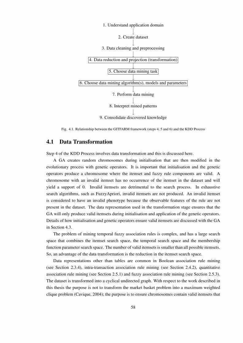
1. Understand application domain
2. Create dataset
3. Data cleaning and preprocessing
4. Data reduction and projection (transformation)
5. Choose data mining task
6. Choose data mining algorithm(s), models and parameters
7. Perform data mining
8. Interpret mined patterns
9. Consolidate discovered knowledge
Fig. 4.1. Relationship between the GITFARM framework (steps 4, 5 and 6) and the KDD Process
4.1 Data Transformation
Step 4 of the KDD Process involves data transformation and this is discussed here.
A GA creates random chromosomes during initialisation that are then modified in the
evolutionary process with genetic operators. It is important that initialisation and the genetic
operators produce a chromosome where the itemset and fuzzy rule components are valid. A
chromosome with an invalid itemset has no occurrence of the itemset in the dataset and will
yield a support of 0. Invalid itemsets are detrimental to the search process. In exhaustive
search algorithms, such as FuzzyApriori, invalid itemsets are not produced. An invalid itemset
is considered to have an invalid phenotype because the observable features of the rule are not
present in the dataset. The data representation used in the transformation stage ensures that the
GA will only produce valid itemsets during initialisation and application of the genetic operators.
Details of how initialisation and genetic operators ensure valid itemsets are discussed with the GA
in Section 4.3.
The problem of mining temporal fuzzy association rules is complex, and has a large search
space that combines the itemset search space, the temporal search space and the membership
function parameter search space. The number of valid itemsets is smaller than all possible itemsets.
So, an advantage of the data transformation is the reduction in the itemset search space.
Data representations other than tables are common in Boolean association rule mining
(see Section 2.3.4), intra-transaction association rule mining (see Section 2.4.2), quantitative
association rule mining (see Section 2.5.1) and fuzzy association rule mining (see Section 2.5.3).
The dataset is transformed into a cyclical undirected graph. With respect to the work described in
this thesis the purpose is not to transform the market basket problem into a maximum weighted
clique problem (Cavique, 2004); the purpose is to ensure chromosomes contain valid itemsets that
58

are present in the dataset and to reduce the itemset search space.
An undirected graph, G, consists of a pair of finite sets (V,E) where V is a non-empty set of
vertices and E is a set of pairs (e, t). Each pair in E consists of an edge, e, and a non-empty finite
set of TIDs, t. Each edge, e, is an unordered pair of vertices (a, b). The definition extends regular
graphs by including a set of TIDs for each edge.
An example is presented to demonstrate the construction of the graph. Table 4.1 is a small
example of a quantitative market basket dataset transformed into the graph of Figure 4.2. Each
edge represents the co-occurrence of two items in a transaction, or one item in a transaction. Items
are vertices. The TIDs of the co-occurrence are also on an edge. Edges are paired with a set of
TIDs to identify the co-occurrence of items. If there is no set of TIDs for an edge then an edge
does not exist.
Table 4.1. Example dataset containing three items (A, B and C) in vertical layout
TID A B C
1 4 6 122 0 2 143 16 11 04 1 0 13
A
B
C
13
12
14
134
123
124
Fig. 4.2. Example graph transformed from dataset in Table 4.1
The vertices and edges for the example graph are defined as
V = {A,B,C},
E = {((A,B), {1, 3}),
((B,C), {1, 2}),
((A,C), {1, 4}),
((A,A), {1, 3, 4}),
((B,B), {1, 2, 3}),
((C,C), {1, 2, 4})}.
59
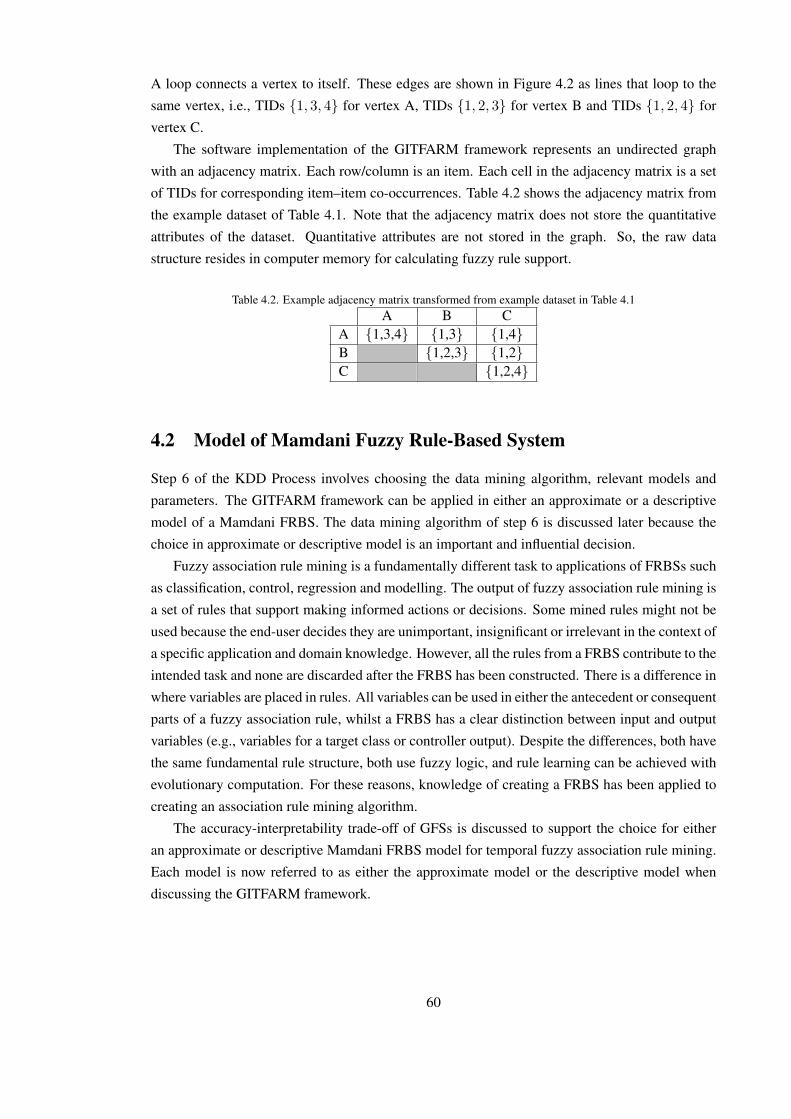
A loop connects a vertex to itself. These edges are shown in Figure 4.2 as lines that loop to the
same vertex, i.e., TIDs {1, 3, 4} for vertex A, TIDs {1, 2, 3} for vertex B and TIDs {1, 2, 4} for
vertex C.
The software implementation of the GITFARM framework represents an undirected graph
with an adjacency matrix. Each row/column is an item. Each cell in the adjacency matrix is a set
of TIDs for corresponding item–item co-occurrences. Table 4.2 shows the adjacency matrix from
the example dataset of Table 4.1. Note that the adjacency matrix does not store the quantitative
attributes of the dataset. Quantitative attributes are not stored in the graph. So, the raw data
structure resides in computer memory for calculating fuzzy rule support.
Table 4.2. Example adjacency matrix transformed from example dataset in Table 4.1A B C
A {1,3,4} {1,3} {1,4}B {1,2,3} {1,2}C {1,2,4}
4.2 Model of Mamdani Fuzzy Rule-Based System
Step 6 of the KDD Process involves choosing the data mining algorithm, relevant models and
parameters. The GITFARM framework can be applied in either an approximate or a descriptive
model of a Mamdani FRBS. The data mining algorithm of step 6 is discussed later because the
choice in approximate or descriptive model is an important and influential decision.
Fuzzy association rule mining is a fundamentally different task to applications of FRBSs such
as classification, control, regression and modelling. The output of fuzzy association rule mining is
a set of rules that support making informed actions or decisions. Some mined rules might not be
used because the end-user decides they are unimportant, insignificant or irrelevant in the context of
a specific application and domain knowledge. However, all the rules from a FRBS contribute to the
intended task and none are discarded after the FRBS has been constructed. There is a difference in
where variables are placed in rules. All variables can be used in either the antecedent or consequent
parts of a fuzzy association rule, whilst a FRBS has a clear distinction between input and output
variables (e.g., variables for a target class or controller output). Despite the differences, both have
the same fundamental rule structure, both use fuzzy logic, and rule learning can be achieved with
evolutionary computation. For these reasons, knowledge of creating a FRBS has been applied to
creating an association rule mining algorithm.
The accuracy-interpretability trade-off of GFSs is discussed to support the choice for either
an approximate or descriptive Mamdani FRBS model for temporal fuzzy association rule mining.
Each model is now referred to as either the approximate model or the descriptive model when
discussing the GITFARM framework.
60

4.2.1 Approximate
The problem of losing some temporal fuzzy association rules is related to the dynamic nature of
the environment and how fuzzy sets represent quantities of items. The flexibility of an approximate
model can overcome this problem by allowing fuzzy sets to be defined anywhere in the universe
of discourse, so they are not fixed. Fuzzy numbers are used in an approximate FRBS model
to represent the quantities of items. For example, a rule could take the form “customers on
a Monday morning who purchased approximately 4.5 pizzas also purchased approximately 15
beers”. Linguistic terms are not present in fuzzy numbers so there is no problem of contextual
meaning associated with linguistic terms. Instead, a change in context is modelled with a fuzzy
number that approximates a different number. A benefit of not using linguistic terms is that the
approximate model does not prescribe preconceptions about linguistic terms.
The benefits of an approximate model relate more to accuracy than interpretability. The
accuracy of an approximate model is crucial for discovering temporal fuzzy association rules,
because accuracy is achieved by flexibility in the rule structure. Figure 4.3 illustrates the
difference between approximate and descriptive membership functions, and their suitability for
either accuracy or interpretability. The descriptive model is discussed in the next section. The
problem with applying traditional fuzzy association rule mining algorithms to temporal datasets
is that the linguistic terms are defined a priori and so the induction of rules is limited to those
linguistic terms. Flexibility is crucial for discovering temporal fuzzy association rules because it
allows rules to be discovered that would otherwise fall on the intersections of membership function
boundaries. A descriptive model that uses linguistic terms has a rigid partitioning of the input and
output spaces that limits the flexibility of rule structure. An approximate model has no rigid
partitions, and removes the problem of rules occurring at the intersection of membership function
boundaries. This flexibility allows an increase in the degrees of freedom and expressiveness of the
rules, because each rule has its own distinct membership functions that are specific to a temporal
period of the dataset.
Mining temporal fuzzy association rules is a complex problem because of the different types
of search space and the size of each search space. An approximate model is good for expressing
temporal patterns because it provides a mechanism to model the fine detail that can be hidden
amongst multiple search spaces. Furthermore, a flexible approach to the definition of fuzzy sets
also allows complex problems to be modelled with as many rules as required. This means that
many temporal patterns with many different fuzzy sets can be discovered.
However, the flexibility of an approximate model creates a lack of semantic-based inter-
pretability because the membership functions are not assigned linguistic labels — they are said
to be semantic free. Instead, fuzzy numbers model approximate quantities. Fuzzy numbers are
less interpretable than linguistic terms. However, fuzzy numbers do describe quantities, albeit in
a different format.
Mining fuzzy association rules with fuzzy numbers has a larger search space than with
descriptive rules. This is a disadvantage for a GA, because the size of the search space increases
Carse et al. (1996).
61

Approx. 3 Approx. 7.5
Aµ
VL L M H VH
B
µ
Accuracy Interpretability
Fig. 4.3. Suitability of approximate (variable A) and descriptive (variable B) membership functions for accuracy andinterpretability
4.2.2 Descriptive
A descriptive model has a rigid partitioning of the input and output spaces that leads to the
problem of losing temporal fuzzy association rules. However, the 2-tuple linguistic representation
can provide a solution to the lack of flexibility in a descriptive model. The 2-tuple linguistic
representation was presented in Section 2.1.1.1 and its use for fuzzy association rule mining has
been reviewed in Section 2.5.3. An example rule, with the 2-tuple linguistic representation, could
take the form “customers on a Monday morning who purchased a (low, 0.1) quantity of pizza also
purchased a (medium, 0.2) quantity of beer”.
The benefit of a descriptive model relates to interpretability rather than accuracy. Sec-
tion 2.2.3.1 of the literature review has shown how context adaptation can be applied as a method of
tuning the accuracy of a FRBS. The crucial benefit of context adaptation was the ability to maintain
the semantic-based interpretability of a linguistic term whilst only slightly changing the meaning.
The 2-tuple linguistic representation adapts the context of a linguistic term by performing a lateral
displacement of a fuzzy set. The lateral displacement provides the rule flexibility required for
mining temporal fuzzy association rules.
The approximate model uses fuzzy numbers in rules so that each rule has its own distinct
membership functions. This principle is relevant to how the 2-tuple linguistic representation is
applied in the descriptive model. Each rule mined from the GITFARM framework has its own
lateral displacements that are specific to the context of each rule. For example, if identical rules
exist, but with different lateral displacements, then the rules are specific to the context of each
rule. Also, if identical rules exist, but with different lateral displacements for different temporal
periods, then the rules are specific to the context of the temporal periods. The application of the
2-tuple linguistic representation is considered to be learning, and not tuning, because the lateral
displacements are specific to each rule produced, so the context is learnt.
As previously mentioned in the data transformation stage of the framework (Section 4.1), the
search space is large and complex. An advantage of the 2-tuple linguistic representation is the
reduction in search space. The 2-tuple linguistic representation has two parameters (linguistic
term and lateral displacement) instead of three parameters of a triangular membership function
for an approximate model. Note that the search space of linguistic terms (nominal data type)
62

is smaller than that of lateral displacement (interval data type). The benefit of a reduced search
space is only applicable to the 2-tuple linguistic representation, and not the descriptive model.
Other representations in the descriptive model may have a different number of parameters and
different data types.
4.3 Genetic Algorithm
The choice of Mamdani FRBS model has been discussed. The remaining part in step 6 of the
KDD Process involves defining the data mining algorithm, which is discussed here.
A GA is chosen for mining temporal fuzzy association rules because the search space is large
and complex. The literature review has shown that an exhaustive search is recognised as being
prohibitive for searching only the membership function parameter space, and that a GA is often
used. The CHC algorithm is selected because CHC has been shown to be very effective in learning
the context of fuzzy association rules (Alcala-Fdez et al., 2009a). CHC has a slow convergence,
so it can run for a long time to achieve high quality solutions (Alcala et al., 2007). Furthermore,
CHC has a good balance between exploration and exploitation, so in complex problems CHC is
less likely to become stuck in local optima.
CHC serves two purposes; CHC simultaneously evolves the temporal fuzzy association
rules and the membership functions. CHC simultaneously performs a discrete (combinatorial)
search for the items in a rule and a continuous search for the membership function parameters.
Simultaneously evolving both parts overcomes the cause of losing temporal fuzzy association rules
where the linguistic terms (and membership function parameters) are defined before the mining
process. This is an important reason why the GITFARM framework is capable of solving the
hypothesised problem.
4.3.1 Chromosome
In the original CHC algorithm a binary representation is used. A mixed representation is required
for temporal fuzzy association rule mining. A chromosome C has mixed types and is defined
using the Michigan representation as
Approximate:C = (el, eu, p1, i1, a1, b1, c1, . . . , pk, ik, ak, bk, ck)
Descriptive:C = (el, eu, p1, i1, s1, α1, . . . , pk, ik, sk, αk)
where el is the lower temporal endpoint, eu is the upper temporal endpoint, p is a flag to determine
the antecedent-consequent part, i is the item (e.g., beer) and k is the number of items in a rule.
For an approximate model, the parameters a, b and c refer to the triangular membership function
parameters. For a descriptive model, s is the linguistic term and α is the lateral displacement
for that term in a rule. A clause in a rule defines a unit of a proposition (defined in Section 4).
63

So a clause of a rule is defined as: the item, membership function parameters and antecedent-
consequent part for an approximate model; and, the item, linguistic term, lateral displacement
and antecedent-consequent part for a descriptive model. A clause is identified as having the same
index where k is the length of a rule.
The following example rules shows the genotype (chromosome) mapping to the phenotype
(rule). Note that the antecedent has a clause index of 2 meaning the antecedent-consequent
parameter for p1 is 0 and p2 is 1, for both approximate and descriptive rules.
Approximate:
For endpoints 0 (el) – 10 (eu)
IF quantity of pizza (i2) is approximately 4.5 (a=3.5, b=4.5, c=5)
THEN quantity of beer (i1) is approximately 15 (a=14, b=15, c=17)
Descriptive:
For endpoints 0 (el) – 10 (eu)
IF quantity of pizza (i2) is (low (s2), 0.1 (α2))
THEN quantity of beer (i1) is (medium (s1), 0.2 (α1))
Minimum temporal granularity restricts the length of the endpoints (i.e., the number of
transactions). Otherwise the GA evolves towards the smallest temporal period because the
temporal fuzzy support (defined next in Section 4.3.2) is higher when relative to one transaction
rather than when relative to two or more transactions. For example, 1 of 10 transactions has a fuzzy
support of 1/10 = 0.1 for a given rule. Without a minimum temporal granularity it is possible for
the GA to evolve endpoints that cover only 1 transaction so the temporal fuzzy support is 1/1 =
1. A rule that covers one transaction is undesirable. Minimum temporal granularity prevents this
problem. Two other restrictions are placed on the temporal endpoints. The maximum temporal
granularity defines the largest temporal period. Temporal granularity defines the granularity of
temporal periods.
Approximate: Soft constrained learning restricts the triangular membership function parameters
of the fuzzy numbers. As discussed in Section 2.2.1, soft constrained learning is a good trade-off
between the flexibility of defining membership functions and the size of the membership function
search space. Soft constrained learning restricts membership function parameters so there is a limit
on the maximum distance between parameters a and c, which is referred to as width. Without soft
constrained learning, the membership functions evolve to cover the entire universe of discourse
because this yields higher fuzzy support, but at the cost of losing semantic-based interpretability.
Figure 4.4 illustrates the constraints applied to the membership functions.
Descriptive: The linguistic labels are modelled with symmetric triangular fuzzy sets, which is the
original proposal of the 2-tuple linguistic representation (Herrera and Martınez, 2000). There is
assumed to be no unbalanced linguistic information that would otherwise require an unbalanced
scale of linguistic terms (Martınez and Herrera, 2012). Lateral displacement is encoded with one
64

b
a c
Quantity
Deg
ree
ofm
embe
rshi
p
Fig. 4.4. Soft constrained learning for membership function parameters in an approximate rule with constraints a <=b <= c
parameter and the advantage is a reduction in the search space of membership function parameters.
Reducing one dimension of the search space is important because it alleviates the increase in
overall search space that arises from the simultaneous need to search for rules, learn the contexts of
membership functions and search the temporal space. However, the flexibility of the membership
function’s shape is reduced, because it is only displaced along the universe of discourse.
Not all items are represented in the chromosome because there can be a large number of
items to consider in real-world applications, particularly market basket applications. So, items are
randomly selected to appear in chromosomes during initialisation and restarts.
Triangular membership functions were used because of their prevalence in fuzzy association
rule mining literature (Kaya et al., 2002; Hong et al., 2008; Alcala-Fdez et al., 2009a) and their
similar performance to other membership function types (Alcala et al., 2007). Other types of
membership function are possible, but the main focus of the hypothesis is to demonstrate how
temporal fuzzy association rules are lost. This loss is caused by temporal patterns occurring at the
intersection of membership function boundaries and so the problem is present in many types of
membership function.
The rules produced from running FuzzyApriori on all datasets showed that all rules had one
clause in the consequent, so the chromosome is restricted to one clause in the consequent. This
is beneficial for complexity-based interpretability because the readability of rules is easier with
fewer clauses/conditions (Gacto et al., 2011).
The graph is not represented in the chromosome. The purpose of the graph is to identify valid
itemsets, which are present in the dataset, and these itemsets are represented in the chromosome.
4.3.2 Fitness Evaluation
Fitness of a chromosome is evaluated by the addition of temporal fuzzy support and weighted
confidence. Temporal fuzzy support divides the fuzzy count of itemsets (Hong et al., 2001) by the
size of a temporal partition (Ale and Rossi, 2000). So temporal fuzzy support measures the fuzzy
support of a rule relative to the size of the temporal period. Temporal fuzzy support models an
exhibition period for a temporal association rule (see Section 2.4.2.4 of the literature review). This
is a preference-based multi-objective approach that maximises the objectives of temporal fuzzy
support and confidence.
65

The fuzzy support count of a chromosome measures the fuzzy support of a rule for one
transaction. The fuzzy support count performs the same measurement on the approximate and
descriptive models, but the definitions of how this is calculated differs slightly because of the
membership functions. The fuzzy support count of a chromosome C in a single transaction tj is
defined from Hong et al. (2001) as
Approximate:
FuzSupTran(C(tj)) =k
minn=1
µf (t(in)j ), (4.1)
Descriptive:
FuzSupTran(C(tj)) =k
minn=1
µ(sm,αn)(t(in)j ), (4.2)
where µ is the degree of membership (calculated for either a fuzzy number (µf ), or a linguistic
label and lateral displacement (µ(sn,αn))) for item in with a rule of length k and for one transaction.
The minimum is used for intersection of all the clauses, which is the same method of intersection
used in FuzzyApriori.
FuzSupTran is then used to calculate fuzzy support counts across multiple transactions and
the fitness is defined in this thesis as
Fitness(C) =
∑euj=el
FuzSupTran(C(tj)X ∩ C
(tj)Y )
eu − el
(4.3)
+w
∑euj=el
FuzSupTran(C(tj)X ∩ C
(tj)Y )∑eu
j=elFuzSupTran(C
(tj)X )
,
where C is a chromosome, X is the rule antecedent, Y is the rule consequent, j is a dataset TID
from the el lower endpoint to the eu upper endpoint, and w is a weight applied to the confidence
measure. Hence, C(tj)X and C
(tj)Y are the rule antecedent and the rule consequent respectively for
one transaction in the dataset. A weight is required to avoid local minima that occur as a result
of the magnitude of confidence being higher than the magnitude of temporal fuzzy support; a GA
produces high confidence values (Matthews et al., 2012; Alcala-Fdez et al., 2010) compared with
a smaller magnitude of support values. For example, a temporal fuzzy support value of 0.001
is smaller than a confidence value of 0.1, so the confidence value has more influence than the
temporal fuzzy support. The weight was determined from multiple runs of the algorithm so that
the temporal fuzzy support and weighted confidence had the same order of magnitude.
A worked example is given for both approximate and descriptive models to demonstrate fitness
evaluation. Consider the example dataset in Table 4.3 and the membership functions of Figure 4.5
and Figure 4.6. The membership functions are assumed to be the same for both items (i.e., pizza
and beer) in this example. The fuzzy support count is calculated for the first TID, i.e., t1, for
both approximate and descriptive models. Values are rounded to 2 significant figures. The fuzzy
support count is then repeated for each transaction in the example dataset to calculate the fuzzy
66

support and confidence. So for the same rules the fitness is calculated as follows.
Table 4.3. Example dataset for demonstrating fitness evaluation
TID Items
1 {cheese(2), pizza(5), beer(15)}2 {pizza(4), beer(16), milk(18)}
1 5 10 15 200
0.5
1 (low, 0.1)(medium, 0.2)(high, 0)
Quantity
Deg
ree
ofm
embe
rshi
p
Fig. 4.5. Membership functions for approximately 4.5and approximately 15
1 5 10 15 200
0.5
1 approx. 4.5 approx. 15
Quantity
Deg
ree
ofm
embe
rshi
p
Fig. 4.6. Membership functions for low, medium andhigh
Approximate: Descriptive:
IF pizza is approximately 4.5 IF pizza is (low, 0.1)
THEN beer is approximately 15 THEN beer is (medium, 0.2)
FuzSupTran(C(t1))=2
minn=1
µf (t(in)1 )
=min(µ4.5(5), µ15(15))
=min(0.5, 1)
=0.5
FuzSupTran(C(t1))=2
minn=1
µ(sn,αn)(t(in)1 )
=min(µ(l,0.1)(5), µ(m,0.2)(15))
=min(0.68, 0.73)
=0.68
FuzSupTran(C(t2))=2
minn=1
µf (t(in)2 )
=min(µ4.5(4), µ15(16))
=min(0.75, 0.5)
=0.5
FuzSupTran(C(t2))=2
minn=1
µ(sn,αn)(t(in)2 )
=min(µ(l,0.1)(4), µ(m,0.2)(16))
=min(0.78, 0.62)
=0.62
FuzSup(C(tj))=
2∑j=1
min(µ4.5(tj), µ15(tj))
2
=
(min(µ4.5(5), µ15(15))+
min(µ4.5(4), µ15(16))
)2
=min(0.5, 1) + min(0.75, 0.5)
2
=0.5 + 0.5
2=0.5
FuzSup(C(tj))=
2∑j=1
min(µ(l,0.1)(tj), µ(m,0.2)(tj))
2
=
(min(µ(l,0.1)(5), µ(m,0.2)(15))+
min(µ(l,0.1)(4), µ(m,0.2)(16))
)2
=min(0.68, 0.73) + min(0.78, 0.62)
2
=0.68 + 0.62
2=1.3
67

Conf(C(tj))=
2∑j=1
min(µ4.5(tj), µ15(tj))
2∑j=1
min(µ4.5(tj))
=
(min(µ4.5(5), µ15(15))+
min(µ4.5(4), µ15(16))
)(min(µ4.5(5))+
min(µ4.5(4))
)
=min(0.5, 1) + min(0.75, 0.5)
min(0.5) + min(0.75)
=0.5 + 0.5
0.5 + 0.75=0.8
Conf(C(tj))=
2∑j=1
min(l,0.1)(tj), µ(m,0.2)(tj))
2∑j=1
min(µ(l,0.1)(tj))
=
(min(µ(l,0.1)(5), µ(m,0.2)(15))+
min(µ(l,0.1)(4), µ(m,0.2)(16))
)(min(µ(l,0.1)(5))+
min(µ(l,0.1)(4))
)
=min(0.68, 0.73) + min(0.78, 0.62)
min(0.68) + min(0.78)
=0.68 + 0.62
0.68 + 0.78=0.89
Fitness(C(tj))=FuzSup(C(tj)) + wConf(C(tj))
=0.5 + w0.8
Fitness(C(tj))=FuzSup(C(tj)) + wConf(C(tj))
=1.3 + w0.89
Note: l is low and m is medium.
4.3.3 Initialisation
The first generation is randomly initialised. Each chromosome requires four parts to be initialised:
the temporal endpoints, items, parameters for either the fuzzy number or lateral displacement, and
antecedent-consequent parameters.
The temporal endpoints are initialised to have a temporal granularity that is between the
minimum and maximum temporal granularity (defined in Section 4.3.1). Initialisation of itemsets
and temporal endpoints requires knowledge of both of these parts to ensure the itemset is present
in a temporal period. Algorithm CreateItemsetAndEndpoints creates the itemset and the temporal
endpoints in a chromosome so that the itemsets are within the temporal endpoints and no items are
duplicated. CreateItemsetAndEndpoints makes use of the graph for looking up transaction IDs,
and the raw data structure for selecting items from a transaction.
Algorithm 1 CreateItemsetAndEndpointsInputs:
k ← Length of itemset;
M ← Adjacency matrix of graph of dataset;
Outputs:
I; // An itemset of length k
(el, eu); // Lower and upper endpoints
Begin
68
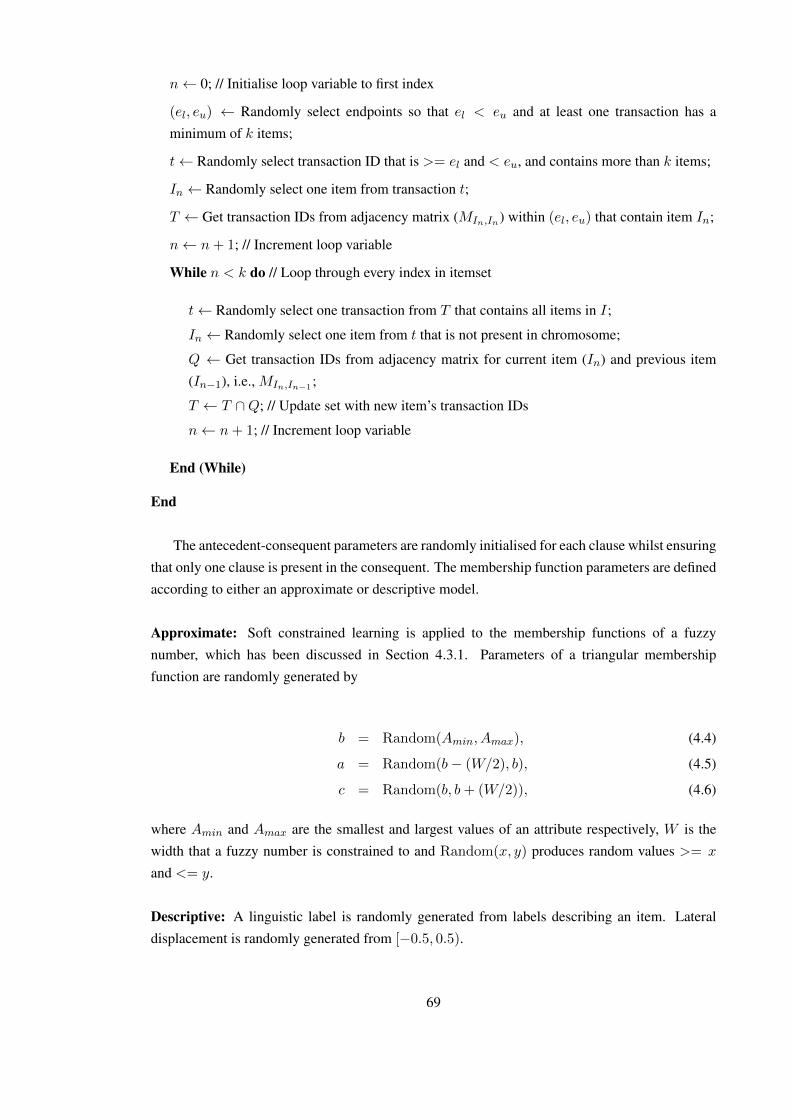
n← 0; // Initialise loop variable to first index
(el, eu) ← Randomly select endpoints so that el < eu and at least one transaction has a
minimum of k items;
t← Randomly select transaction ID that is >= el and < eu, and contains more than k items;
In ← Randomly select one item from transaction t;
T ← Get transaction IDs from adjacency matrix (MIn,In) within (el, eu) that contain item In;
n← n+ 1; // Increment loop variable
While n < k do // Loop through every index in itemset
t← Randomly select one transaction from T that contains all items in I;
In ← Randomly select one item from t that is not present in chromosome;
Q ← Get transaction IDs from adjacency matrix for current item (In) and previous item
(In−1), i.e., MIn,In−1 ;
T ← T ∩Q; // Update set with new item’s transaction IDs
n← n+ 1; // Increment loop variable
End (While)
End
The antecedent-consequent parameters are randomly initialised for each clause whilst ensuring
that only one clause is present in the consequent. The membership function parameters are defined
according to either an approximate or descriptive model.
Approximate: Soft constrained learning is applied to the membership functions of a fuzzy
number, which has been discussed in Section 4.3.1. Parameters of a triangular membership
function are randomly generated by
b = Random(Amin, Amax), (4.4)
a = Random(b− (W/2), b), (4.5)
c = Random(b, b+ (W/2)), (4.6)
where Amin and Amax are the smallest and largest values of an attribute respectively, W is the
width that a fuzzy number is constrained to and Random(x, y) produces random values >= x
and <= y.
Descriptive: A linguistic label is randomly generated from labels describing an item. Lateral
displacement is randomly generated from [−0.5, 0.5).
69
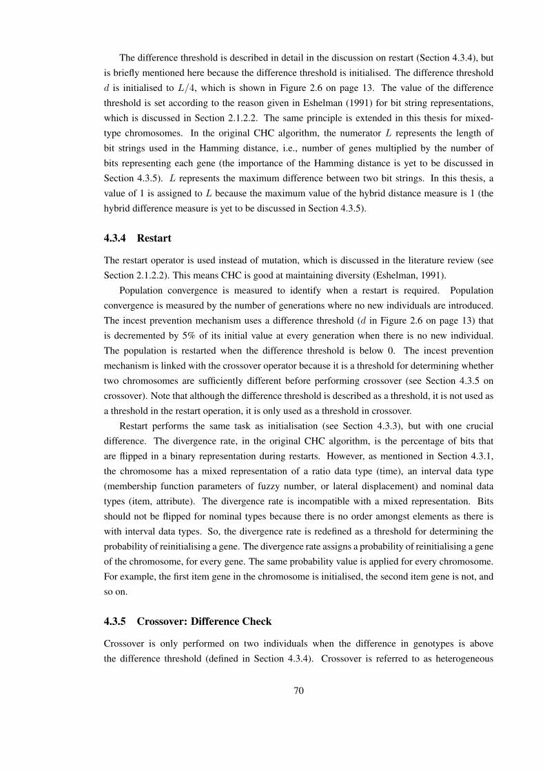
The difference threshold is described in detail in the discussion on restart (Section 4.3.4), but
is briefly mentioned here because the difference threshold is initialised. The difference threshold
d is initialised to L/4, which is shown in Figure 2.6 on page 13. The value of the difference
threshold is set according to the reason given in Eshelman (1991) for bit string representations,
which is discussed in Section 2.1.2.2. The same principle is extended in this thesis for mixed-
type chromosomes. In the original CHC algorithm, the numerator L represents the length of
bit strings used in the Hamming distance, i.e., number of genes multiplied by the number of
bits representing each gene (the importance of the Hamming distance is yet to be discussed in
Section 4.3.5). L represents the maximum difference between two bit strings. In this thesis, a
value of 1 is assigned to L because the maximum value of the hybrid distance measure is 1 (the
hybrid difference measure is yet to be discussed in Section 4.3.5).
4.3.4 Restart
The restart operator is used instead of mutation, which is discussed in the literature review (see
Section 2.1.2.2). This means CHC is good at maintaining diversity (Eshelman, 1991).
Population convergence is measured to identify when a restart is required. Population
convergence is measured by the number of generations where no new individuals are introduced.
The incest prevention mechanism uses a difference threshold (d in Figure 2.6 on page 13) that
is decremented by 5% of its initial value at every generation when there is no new individual.
The population is restarted when the difference threshold is below 0. The incest prevention
mechanism is linked with the crossover operator because it is a threshold for determining whether
two chromosomes are sufficiently different before performing crossover (see Section 4.3.5 on
crossover). Note that although the difference threshold is described as a threshold, it is not used as
a threshold in the restart operation, it is only used as a threshold in crossover.
Restart performs the same task as initialisation (see Section 4.3.3), but with one crucial
difference. The divergence rate, in the original CHC algorithm, is the percentage of bits that
are flipped in a binary representation during restarts. However, as mentioned in Section 4.3.1,
the chromosome has a mixed representation of a ratio data type (time), an interval data type
(membership function parameters of fuzzy number, or lateral displacement) and nominal data
types (item, attribute). The divergence rate is incompatible with a mixed representation. Bits
should not be flipped for nominal types because there is no order amongst elements as there is
with interval data types. So, the divergence rate is redefined as a threshold for determining the
probability of reinitialising a gene. The divergence rate assigns a probability of reinitialising a gene
of the chromosome, for every gene. The same probability value is applied for every chromosome.
For example, the first item gene in the chromosome is initialised, the second item gene is not, and
so on.
4.3.5 Crossover: Difference Check
Crossover is only performed on two individuals when the difference in genotypes is above
the difference threshold (defined in Section 4.3.4). Crossover is referred to as heterogeneous
70

re-combination in CHC because the parent chromosomes must be sufficiently different. The
method for evaluating the difference in chromosomes is presented first followed by the method
for performing crossover.
In the original CHC algorithm, the Hamming distance (Hamming, 1950) evaluates the
difference between two bit strings. However, as mentioned in Section 4.3.1, the chromosome
has a mixed representation of a ratio data type (time), an interval data type (membership function
parameters of fuzzy number or lateral displacement) and nominal data types (item, attribute). To
allow the Hamming distance to be used, the interval data types (membership function parameters
of fuzzy number or lateral displacement) are converted into a Gray code (Gray, 1953). Such an
approach has shown good performance in Alcala et al. (2007) and Alcala-Fdez et al. (2009a) where
CHC learnt lateral displacements with the 2-tuple linguistic representation for fuzzy control and
fuzzy association rule mining.
For coherence, the Hamming distance is only evaluated for membership functions when the
clauses are the same. It is unsuitable to calculate the Hamming distance between two membership
functions of different items because they have different semantics. For example, the linguistic
terms for quantities of pizza and beer may be different because the perspectives of the quantities
for those specific items are different. Each clause in a rule is checked to identify if a clause’s
content is the same as the clause from the other chromosome. This is performed differently for the
approximate and descriptive models, each are defined below.
The chromosome only represents items in the rule, and not every possible item in the dataset.
So it is possible for the same item to exist in both parent chromosomes, but at different loci. This
is a problem when using the Hamming distance because a bitwise comparison is performed at
each locus in a bit string. To overcome this problem, all matching genes are temporarily (only
for purpose of calculating Hamming distance) moved to the same loci to ensure the Hamming
distance is semantically correct. After the genes are moved, comparisons are then made.
Approximate: For coherence, membership function parameters are only compared using the
Hamming distance when the clauses have the same antecedent-consequent parameter and item.
If a clause does not match, then the maximum difference in Gray Code is assigned for each
chromosome (e.g., all 0s for one chromosome and all 1s for the other).
Descriptive: For coherence, lateral displacements are only compared, using the Hamming
distance, when the clauses have the same antecedent-consequent parameter, item and linguistic
term. If a clause does not match, then the maximum difference in Gray Code is assigned for each
chromosome (e.g., all 0s for one chromosome and all 1s for the other).
The Hamming distance is defined as
H(f, g) =1
q
q∑n=1
δ(fn, gn), (4.7)
where f and g are Gray Codes of bit strings with length q and a position in a bit string is n. The
71

term δ is an exclusive XOR operation defined as
δ(x, y) =
0 (x > 0 ∧ y > 0) ∨ (x = 0 ∧ y = 0),
1 otherwise.(4.8)
So a clause is considered to be a nominal type when it contains an item, a linguistic label (only
for descriptive model) and an antecedent-consequent parameter. In order to define the Jaccard
distance, the Jaccard coefficient is defined as
J(A,B) =|A ∩B||A ∪B|
, (4.9)
where A and B are sets of tuples for either: i) temporal endpoint; ii) an antecedent-consequent
parameter and an item for an approximate model; or iii) an antecedent-consequent parameter, an
item, and a linguistic label for a descriptive model. The Jaccard distance is defined as
J ′(A,B) = 1− J(A,B). (4.10)
The Hamming distance and the Jaccard distance evaluate the different genes of parent
chromosomes according to either an approximate or descriptive model. Each measure is
normalised and aggregated.
Approximate: The following measures are aggregated using the arithmetic mean: the
Hamming distance of the temporal endpoints (el, eu), the sum of all Jaccard distances of
(p(antecedent-consequent parameter), i(item)) tuples and the sum of all Hamming distances
of membership function parameters of fuzzy numbers (a, b, c). The temporal endpoints are
concatenated in the order they appear in the chromosome and so are the membership function
parameters. The hybrid difference measure h, for two chromosomes C1 and C2 of an approximate
model, is defined as
h =1
3
(H(gray(C1(el,eu)), gray(C2(el,eu)))
g
+1
k
k∑n=1
J ′(C1(in,pn), C2(in,pn))
+1
k
k∑n=1
H(gray(C1(an,bn,cn)), gray(C2(an,bn,cn)))
g
), (4.11)
where g is the number of bits for representing the Gray Code. For example, assuming 30 bits are
used in the Gray Code for two hypothetical rules:
72

C1 = (0, 10, pizza, 2.5, 4.5, 5.5, 0,beer, 14, 15, 17, 1)
C2 = (0, 10, pizza, 2.5, 4.5, 5.5, 0,beer, 10, 11, 13, 1)
h=1
3
(H(C1(0,10), C2(0,10))
30
+1
2(J ′(C1(pizza,0), C2(pizza,0)) + J ′(C1(beer,1), C2(beer,1)))
+1
2
(H(gray(C1(2.5,4.5,5.5)), gray(C2(2.5,4.5,5.5)))
30+
H(gray(C1(14,15,17)), gray(C2(10,11,13)))
30
))=
1
3
(30
30+
1
2(1 + 1) +
1
2
(30
30+
0
30
))=
1
3(1 + 1 + 0.5)
= 0.83
Descriptive: The following measures are aggregated using the arithmetic mean: the Hamming dis-
tance of the endpoints, the sum of all Jaccard distances of (a(antecedent-consequent parameter),
i(item), s(linguistic label)) tuples and the sum of all Hamming distances of lateral displacements.
The hybrid difference measure h, for two chromosomes C1 and C2 of a descriptive model, is
defined as
h =1
3
(H(gray(C1(el,eu)), gray(C2(el,eu)))
g
+1
k
k∑n=1
J ′(C1(in,sn,pn), C2(in,sn,pn))
+1
k
k∑n=1
H(gray(C1(αn)), gray(C2(αn)))
g
), (4.12)
where g is the number of bits for representing the Gray Code. For example, assuming 3
membership functions with uniform partitioning across a domain of [1, 20] and 30 bits are used in
the Gray Code:
73

C1 = (0, 10,pizza, low, 0.1, 0, beer,medium, 0.5, 1)
C2 = (0, 10,pizza, low, 0.1, 0, beer,medium,−0.3, 1)
h =1
3
(H(C1(0,10), C2(0,10))
30
+1
2(J ′(C1(pizza,low,0), C2(pizza,low,0)) + J ′(C1(beer,medium,1), C2(beer,medium,1)))
+1
2
(H(gray(C1(0.1)), gray(C2(0.1)))
30+
H(gray(C1(0.5)), gray(C2(−0.5)))
30
))=
1
3
(30
30+
1
2(1 + 1) +
1
2
(30
30+
0
30
))=
1
3(1 + 1 + 0.5)
= 0.83
When h < d for two chromosomes, for either an approximate or a descriptive model, they are
sufficiently different so crossover is performed.
4.3.6 Crossover: HybridCrossover
The method for performing crossover is now presented. HybridCrossover is an algorithm that
applies suitable operators to genes that have different data types. The crossover operators are
applied to the genes according to the following.
Approximate:
C = (el, eu, p1, i1︸ ︷︷ ︸swap
,
PCBLX-α︷ ︸︸ ︷a1, b1, c1, . . . , pk, ik︸ ︷︷ ︸
swap
,
PCBLX-α︷ ︸︸ ︷ak, bk, ck)
Descriptive:
C = (el, eu, p1, i1, s1︸ ︷︷ ︸swap
,
PCBLX-α︷︸︸︷α1 , . . . , pk, ik, sk︸ ︷︷ ︸
swap
,
PCBLX-α︷︸︸︷αk )
HybridCrossover does not apply a crossover operator to the temporal endpoints because the
itemsets for temporal endpoints of offspring might not be valid. For example, a rule from
one temporal period might not contain any items in a rule from another temporal period. To
ensure the itemset is valid, the endpoints remain the same during crossover and new temporal
endpoints can be introduced during restart operations. For nominal data types, i.e., antecedent-
consequent parameter, item and linguistic label, the genes are swapped. For interval types, i.e.,
membership function parameters of fuzzy numbers and lateral displacements, the parent centric
BLX-α (PCBLX-α) (Lozano et al., 2004) crossover operator is applied.
Both approximate and descriptive models use PCBLX-α. The descriptive model performs
crossover on each lateral displacement gene in a descriptive model. PCBLX-α is performed as
74
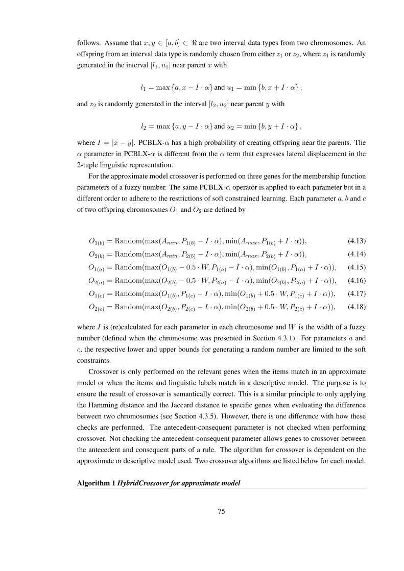
follows. Assume that x, y ∈ [a, b] ⊂ < are two interval data types from two chromosomes. An
offspring from an interval data type is randomly chosen from either z1 or z2, where z1 is randomly
generated in the interval [l1, u1] near parent x with
l1 = max {a, x− I · α} and u1 = min {b, x+ I · α} ,
and z2 is randomly generated in the interval [l2, u2] near parent y with
l2 = max {a, y − I · α} and u2 = min {b, y + I · α} ,
where I = |x − y|. PCBLX-α has a high probability of creating offspring near the parents. The
α parameter in PCBLX-α is different from the α term that expresses lateral displacement in the
2-tuple linguistic representation.
For the approximate model crossover is performed on three genes for the membership function
parameters of a fuzzy number. The same PCBLX-α operator is applied to each parameter but in a
different order to adhere to the restrictions of soft constrained learning. Each parameter a, b and c
of two offspring chromosomes O1 and O2 are defined by
O1(b) = Random(max(Amin, P1(b) − I · α),min(Amax, P1(b) + I · α)), (4.13)
O2(b) = Random(max(Amin, P2(b) − I · α),min(Amax, P2(b) + I · α)), (4.14)
O1(a) = Random(max(O1(b) − 0.5 ·W,P1(a) − I · α),min(O1(b), P1(a) + I · α)), (4.15)
O2(a) = Random(max(O2(b) − 0.5 ·W,P2(a) − I · α),min(O2(b), P2(a) + I · α)), (4.16)
O1(c) = Random(max(O1(b), P1(c) − I · α),min(O1(b) + 0.5 ·W,P1(c) + I · α)), (4.17)
O2(c) = Random(max(O2(b), P2(c) − I · α),min(O2(b) + 0.5 ·W,P2(c) + I · α)), (4.18)
where I is (re)calculated for each parameter in each chromosome and W is the width of a fuzzy
number (defined when the chromosome was presented in Section 4.3.1). For parameters a and
c, the respective lower and upper bounds for generating a random number are limited to the soft
constraints.
Crossover is only performed on the relevant genes when the items match in an approximate
model or when the items and linguistic labels match in a descriptive model. The purpose is to
ensure the result of crossover is semantically correct. This is a similar principle to only applying
the Hamming distance and the Jaccard distance to specific genes when evaluating the difference
between two chromosomes (see Section 4.3.5). However, there is one difference with how these
checks are performed. The antecedent-consequent parameter is not checked when performing
crossover. Not checking the antecedent-consequent parameter allows genes to crossover between
the antecedent and consequent parts of a rule. The algorithm for crossover is dependent on the
approximate or descriptive model used. Two crossover algorithms are listed below for each model.
Algorithm 1 HybridCrossover for approximate model
75

Inputs:
k ← Length of rule;
P ← Two parent chromosomes;
Outputs:
O; // Two offspring chromosomes
Begin
n← 0; // Initialise loop variable to first index
O ← P ; // Create offsprings from identical copies of parents;
If O have matching items Then
Move clauses, containing matching items, to same loci;
End (If)
While n < k do // Loop through every index in rule
If O items are identical Then
Uniform crossover of membership function parameters of fuzzy number using PCBLX-α;
Uniform crossover of antecedent-consequent parameter using swap;
End (If)
If O items are not identical Then
If O1 is present in endpoints of O2 using Algorithm CheckGraph AND O2 is present in
endpoints of O1 using Algorithm CheckGraph Then
Uniform crossover of {item, membership function parameters of fuzzy number}using swap;
Uniform crossover of antecedent-consequent parameter using swap;
End (If)
End (If)
n← n+ 1; // Increment loop variable
End (While)
End
Algorithm 2 HybridCrossover for descriptive modelInputs:
k ← Length of rule;
P ← Two parent chromosomes;
76
Outputs:
O; // Two offspring chromosomes
Begin
n← 0; // Initialise loop variable to first index
O ← P ; // Create offsprings from identical copies of parents;
If offspring have matching items Then
Move clauses, containing matching items, to same loci;
End (If)
While n < k do // Loop through every index in rule
If O items are identical AND linguistic labels are identical Then
Uniform crossover of lateral displacement using PCBLX-α;
Uniform crossover of antecedent-consequent parameter using swap;
End (If)
If O items are identical AND linguistic labels are not identical Then
Uniform crossover of {linguistic label, lateral displacement} using swap;
Uniform crossover of antecedent-consequent parameter using swap;
End (If)
If O items are not identical Then
If O1 is present in endpoints of O2 using Algorithm CheckGraph AND O2 is present in
endpoints of O1 using Algorithm CheckGraph Then
Uniform crossover of {item, linguistic label, lateral displacement} using swap;
Uniform crossover of antecedent-consequent parameter using swap;
End (If)
End (If)
n← n+ 1; // Increment loop variable
End (While)
End
In the HybridCrossover, for both the approximate and descriptive models, if the items to be
swapped are different then a check is performed before swapping the items. The purpose is to
prevent crossover from producing invalid itemsets. Potential offspring are first checked to identify
if the resulting itemsets are present in the specific temporal partitions of the dataset. If the resulting
offspring are not present then the items are not swapped. Algorithm CheckGraph uses the graph
77

data structure to ensure offspring are valid itemsets in a temporal period. Algorithm CheckGraph
is defined below.
Algorithm 3 CheckGraphInputs:
k ← Length of itemset to be checked;
I ← Itemset to be checked;
j ← Candidate item from itemset I that is to be checked;
M ← Adjacency matrix of graph of dataset;
(el, eu)← Lower and upper endpoints of temporal period;
Outputs:
TRUE or FALSE
Begin
n← 0; // Initialise loop variable to first index
T ← ∅; // Initialise set of transactions to the empty set
p← Clause index of candidate item j;
While n < k do // Loop through every index in itemset
// If index of candidate item not equal to current index
If n 6= p Then
// If T used for first time
If n = 0 OR p = 0 Then
// Initialise
T ←MIn,j that are >= el and < eu;
Else
T ← T ∩MIn,j ; // Update transaction IDs set with transactions containing candidate
item (j) and current item (In)
End (If)
End (If)
n← n+ 1; // Increment loop variable
End (While)
If T = ∅ Then return FALSE;
Else return TRUE;
End (If)
End
78
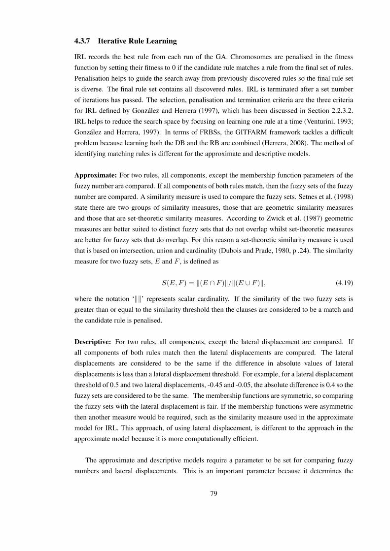
4.3.7 Iterative Rule Learning
IRL records the best rule from each run of the GA. Chromosomes are penalised in the fitness
function by setting their fitness to 0 if the candidate rule matches a rule from the final set of rules.
Penalisation helps to guide the search away from previously discovered rules so the final rule set
is diverse. The final rule set contains all discovered rules. IRL is terminated after a set number
of iterations has passed. The selection, penalisation and termination criteria are the three criteria
for IRL defined by Gonzalez and Herrera (1997), which has been discussed in Section 2.2.3.2.
IRL helps to reduce the search space by focusing on learning one rule at a time (Venturini, 1993;
Gonzalez and Herrera, 1997). In terms of FRBSs, the GITFARM framework tackles a difficult
problem because learning both the DB and the RB are combined (Herrera, 2008). The method of
identifying matching rules is different for the approximate and descriptive models.
Approximate: For two rules, all components, except the membership function parameters of the
fuzzy number are compared. If all components of both rules match, then the fuzzy sets of the fuzzy
number are compared. A similarity measure is used to compare the fuzzy sets. Setnes et al. (1998)
state there are two groups of similarity measures, those that are geometric similarity measures
and those that are set-theoretic similarity measures. According to Zwick et al. (1987) geometric
measures are better suited to distinct fuzzy sets that do not overlap whilst set-theoretic measures
are better for fuzzy sets that do overlap. For this reason a set-theoretic similarity measure is used
that is based on intersection, union and cardinality (Dubois and Prade, 1980, p .24). The similarity
measure for two fuzzy sets, E and F , is defined as
S(E,F ) = ‖(E ∩ F )‖/‖(E ∪ F )‖, (4.19)
where the notation ‘‖‖’ represents scalar cardinality. If the similarity of the two fuzzy sets is
greater than or equal to the similarity threshold then the clauses are considered to be a match and
the candidate rule is penalised.
Descriptive: For two rules, all components, except the lateral displacement are compared. If
all components of both rules match then the lateral displacements are compared. The lateral
displacements are considered to be the same if the difference in absolute values of lateral
displacements is less than a lateral displacement threshold. For example, for a lateral displacement
threshold of 0.5 and two lateral displacements, -0.45 and -0.05, the absolute difference is 0.4 so the
fuzzy sets are considered to be the same. The membership functions are symmetric, so comparing
the fuzzy sets with the lateral displacement is fair. If the membership functions were asymmetric
then another measure would be required, such as the similarity measure used in the approximate
model for IRL. This approach, of using lateral displacement, is different to the approach in the
approximate model because it is more computationally efficient.
The approximate and descriptive models require a parameter to be set for comparing fuzzy
numbers and lateral displacements. This is an important parameter because it determines the
79

degree of overlap between two fuzzy sets that is used for penalising rules during evolution. If
there is a high degree of overlap then the final rule set can contain very similar rules. If there is a
low degree of overlap then some rules may be penalised when there temporal fuzzy support and
confidence may be important to a domain expert.
The rule length is fixed in one run of the GA. The rule length in IRL is configurable to allow
different length rules in the final rule set. Percentages of IRL iterations with specific rule lengths
are assigned. For example, in 100 iterations, 75% could be allocated to rules of length 2 and the
remaining 25% search for rules of length 3. The rule length is fixed in a chromosome, for each
iteration of IRL, otherwise rules evolve to have the minimum length. Fewer clauses in a rule yield
higher temporal fuzzy support values because smaller rules form the building blocks of larger
rules (i.e., the downward closure property in Boolean association rule mining). Furthermore, a
flexible configuration of rule lengths provides a fair comparison with existing approaches, which
is discussed further in Section 5.2.7.
4.4 Discussion
The GITFARM framework has been presented in this chapter. GITFARM is a framework for
mining intra-transaction temporal fuzzy association rules. The GITFARM framework comprises
three components that justify the decision for GITFARM to be a framework. Three steps of the
KDD Process relate to the GITFARM framework.
The first component of the GITFARM framework transforms the dataset from a table into
a graph. The purpose of this component is to use a data structure that explicitly represents the
co-occurrence of items in the dataset. The GA uses the graph to ensure that candidate rules exist
in the dataset. Without the graph structure, it would be possible for the GA to generate rules that
do not exist, non-existing rules are considered to be invalid.
The second component is the choice of model; either approximate or descriptive. The
approximate and descriptive models relate to FRBSs and the fuzzy sets used. The approximate
model provides flexibility in the membership functions so that temporal patterns can be discovered.
The descriptive model provides flexibility in the membership functions, but whilst maintaining the
interpretability of the membership function with a linguistic term. There is a trade-off between the
accuracy and interpretability when choosing between an approximate or descriptive model, for the
GITFARM framework.
The third component is the search method for mining intra-transaction temporal fuzzy
association rules. CHC is the type of GA used. The decision on the approximate/descriptive model
is important because there are small changes in CHC for handling the membership functions that
reflect the choice of model. CHC simultaneously searches for rules and membership functions.
The metaheuristic approach for discovering rules does not guarantee that lost rules are
discovered. The metaheuristic approach may discover rules already discovered with another
approach. In the following chapter a methodology is presented for analysing the ability of this
framework at discovering lost rules.
80

Chapter 5
Experimental Methodology
The GITFARM framework has been proposed as a solution to the hypothesised problem. The
comparative analysis framework is a methodology for testing the hypothesis. The comparative
analysis framework runs the GITFARM framework and a traditional approach. The rules from
both approaches are compared and analysed to verify the hypothesis.
The comparative analysis is presented first in Section 5.1. The variables configured with the
comparative analysis are then discussed in Section 5.2. These include variables for the GITFARM
framework, the traditional approach and the comparative analysis framework.
5.1 Comparative Analysis Framework
The aim of the comparison is to explore the ability of the GITFARM framework to discover intra-
transaction fuzzy association rules that might be lost with a traditional approach. The comparative
analysis framework directly compares both approaches. The concept behind the comparative
analysis framework is to compare rules found by the GITFARM framework with the traditional
approach so that matching rules are identified. The comparison identifies what rules the GITFARM
framework has discovered that were not discovered by the traditional approach.
The comparative analysis framework is created to allow for two search algorithms to be
analysed. The comparative analysis framework has three components that relate to three steps in
the KDD Process, which is shown in Figure 5.1. The figure illustrates how the three components
align with three steps of the KDD Process. Each component of the comparative analysis
framework is now discussed.
5.1.1 Define Model and Parameters
The first component of the comparative analysis framework (step 6 of the KDD Process) is to
choose the data mining algorithm(s), models and parameters. For the purposes of investigating the
hypothesis, the GITFARM framework and the traditional approach are chosen as the data mining
algorithms. As discussed in Section 4.2, the model in the GITFARM framework can be either
approximate or descriptive. Another choice for the model is the linguistic labels for modelling
perceptions such as a quantity, for market basket datasets, and time, for Web log datasets. After
defining the linguistic labels, the membership function parameters are defined. The models and
81
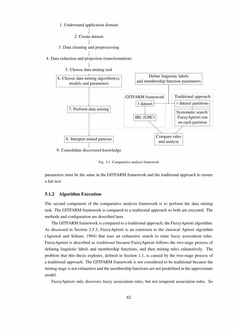
Define linguistic labelsand membership function parameters
1 dataset
IRL (CHC)
r dataset partitions
Systematic search:FuzzyApriori runon each partition
Compare rulesand analyse
GITFARM framework Traditional approach
1. Understand application domain
2. Create dataset
3. Data cleaning and preprocessing
4. Data reduction and projection (transformation)
5. Choose data mining task
6. Choose data mining algorithm(s),models and parameters
7. Perform data mining
8. Interpret mined patterns
9. Consolidate discovered knowledge
Fig. 5.1. Comparative analysis framework
parameters must be the same in the GITFARM framework and the traditional approach to ensure
a fair test.
5.1.2 Algorithm Execution
The second component of the comparative analysis framework is to perform the data mining
task. The GITFARM framework is compared to a traditional approach so both are executed. The
methods and configuration are described here.
The GITFARM framework is compared to a traditional approach, the FuzzyApriori algorithm.
As discussed in Section 2.5.3, FuzzyApriori is an extension to the classical Apriori algorithm
(Agrawal and Srikant, 1994) that uses an exhaustive search to mine fuzzy association rules.
FuzzyApriori is described as traditional because FuzzyApriori follows the two-stage process of
defining linguistic labels and membership functions, and then mining rules exhaustively. The
problem that this thesis explores, defined in Section 1.1, is caused by the two-stage process of
a traditional approach. The GITFARM framework is not considered to be traditional because the
mining stage is not exhaustive and the membership functions are not predefined in the approximate
model.
FuzzyApriori only discovers fuzzy association rules, but not temporal association rules. So
82
to mine temporal fuzzy association rules with FuzzyApriori a systematic search of the temporal
space is conducted. For example, partitioning a dataset containing a week of data, according to
the day, would create seven datasets that FuzzyApriori is then applied to. The rules produced
from FuzzyApriori on each dataset partition are then aggregated into a final rule set. Applying
an exhaustive search method to multiple partitions is similar to cyclic association rule mining
demonstrated by Ozden et al. (1998). When referring to FuzzyApriori in the experimentation of
this thesis, it should be noted that FuzzyApriori is conducted with a systematic search of a dataset,
and not the entire dataset.
Figure 5.1 illustrates the difference in how the datasets are used by the GITFARM framework
and FuzzyApriori. The GITFARM framework is applied directly on the dataset, but FuzzyApriori
is applied to many smaller subsets of the same dataset that has been partitioned.
Fuzzy support is a measure used in FuzzyApriori to analyse the frequency of a rule.
FuzzyApriori is applied in a systematic search of the temporal space, so FuzzyApriori is referred
to as having temporal fuzzy support because the fuzzy support is relative to one temporal
partition. Minimum temporal fuzzy support extends minimum fuzzy support (see Section 2.5.3)
to incorporate the temporal aspect. Temporal fuzzy support is an identical measure used in both
the GITFARM framework and the systematic search with FuzzyApriori. Minimum confidence is
the same.
Note that partitioning the dataset is considered to be different to step 3 of the KDD Process,
which focuses on data cleaning and preprocessing, because the only purpose of partitioning is to
perform a comparative analysis. Also, partitioning the dataset is specific to the approach of how
the FuzzyApriori algorithm is applied and partitioning the dataset may not be required with other
association rule mining algorithms/approaches.
The GITFARM framework and FuzzyApriori can be substituted for other approaches in the
comparative analysis framework. The GITFARM framework is chosen because it is the focus
of this thesis. The literature review identified algorithms that mine temporal patterns in fuzzy
association rules, but none that have an intra-transactional pattern of an exhibition period. The
literature review did not identify an algorithm that mines fuzzy association rules that have an
exhibition period temporal pattern. A logical alternative is to perform a systematic search of
the temporal space and apply an exhaustive search method on each partition. FuzzyApriori was
chosen as the exhaustive search algorithm because it is based on a seminal algorithm in the field
of association rule mining, i.e., the Apriori algorithm. Alternatives are available that can offer
enhanced performance such as those discussed in the literature review (Section 2.5.3), i.e., Fuzzy
Apriori-T and FFP-growth. However, enhancing algorithm performance is not the focus of the
hypothesis.
5.1.3 Rule Analysis
When both approaches for temporal fuzzy association rule mining have been completed, the
third component of the comparative analysis framework compares the rules mined using both
approaches. The purpose is to interpret the results, which is step 8 of the KDD Process, to support
83

the hypothesis. Rules mined with both approaches are compared to identify whether there are new
rules mined with the GITFARM framework that were not mined with FuzzyApriori.
The method for comparing the rules is the same as the method used for IRL in Section 4.3.7.
Each part of a clause is compared between two rules and if all the clauses match then the rules are
the same. For an approximate model, a fuzzy similarity measure compares fuzzy numbers based
on intersection, union and cardinality (Dubois and Prade, 1980, p.24). For a descriptive model,
the lateral displacements of membership functions are compared. Both models apply a threshold
to the measures.
Comparing rules in the descriptive model involves identifying linguistic terms that match.
However, the same method is not possible with the approximate approach because fuzzy numbers
do not have linguistic terms. So to compare fuzzy sets between the approximate and descriptive
models, the descriptive fuzzy set that best matches the approximate fuzzy set is identified. The
matching for an approximate model is done in two stages. First, the descriptive fuzzy sets that
overlap with the approximate fuzzy set are identified. Second, the most similar descriptive fuzzy
set, from the overlapping fuzzy sets, is then identified and this is the descriptive fuzzy set that is
used in the comparison. For example, the fuzzy number approximately 12 forms a clause of a rule
from the GITFARM framework that is to be compared with rules from FuzzyApriori. Figure 5.2
illustrates three fuzzy sets with linguistic terms for the descriptive model, and one fuzzy number
for the approximate model. The fuzzy number, approximately 12, overlaps with the medium and
high fuzzy sets. Of the medium and high fuzzy sets, approximately 12 is more similar to medium.
So the medium fuzzy set is used for making comparisons for a particular clause in a rule. For
remaining clauses in a rule, the process is repeated to identify the most similar fuzzy set.
1 200
0.5
1 Low Medium High
Approx. 12
Quantity
Deg
ree
ofm
embe
rshi
p
Fig. 5.2. Overlapping approximate/descriptive membership functions
A rule from the GITFARM framework that matches a rule from FuzzyApriori is not considered
to be a new rule. In this case, FuzzyApriori is capable of discovering the rule and it is not
considered to be lost. A rule from the GITFARM framework that does not match any rules from
FuzzyApriori is considered to be a new rule. In this case, only the GITFARM framework can
discover the rule. A lost rule is a rule that is only discovered with the GITFARM framework,
i.e., it is new, and satisfies both minimum thresholds. If a temporal fuzzy association rule exists
in a dataset then it is possible for FuzzyApriori to discover it when the minimum temporal fuzzy
support and minimum confidence measures are sufficiently low so the rule would not be discarded.
For existing and new temporal fuzzy association rules the difference in temporal fuzzy support and
confidence measures can be analysed to ascertain the performance of the GITFARM framework.
84
5.2 Variables
The design of the comparative analysis framework is intended to facilitate a fair comparison of the
two approaches in order to support the hypothesis. However, the configuration of the comparative
analysis is crucial for a fair comparison. The comparative analysis framework has dependent
variables that affect the comparison. These variables are described here to justify the setup of the
experiments for a fair comparison of the GITFARM framework and FuzzyApriori. Any variables
that were changed in an experiment are stated in the results.
The GITFARM framework and FuzzyApriori were implemented in Java within the Knowledge
Extraction based on Evolutionary Learning (KEEL) tool (Alcala-Fdez et al., 2009b, 2011). The
experiments were conducted on a personal computer with a 32-bit 2.80GHz dual-core processor
and 4GB RAM.
5.2.1 GITFARM Parameters
All parameters for CHC were determined empirically and are specified here. Experiments were
run with initial parameters and then tuned by hand from observing the results. The population size
was set to 50. The population size is relatively small, but the restart approach is more beneficial
than a larger population (Eshelman, 1991). The divergence rate was set to 0.35, which is the
probability of reinitialising a gene when performing a restart. The α term in PCBLX-α was set
to 1.0, which is the maximum value. Temporal granularity was 100 for the IBM dataset and 3600
seconds the for EPA dataset. The confidence weight w in the fitness function was set to 0.001 for
both approximate and descriptive models with both the EPA dataset and the set of IBM datasets.
The termination criterion for CHC was set to 50000 fitness evaluations. The number of iterations
in IRL was set to 200 for all experiments. The number of rules in IRL assigned to different rule
lengths is stated in the results for different experiments. The temporal granularity was set to the
same values of minimum temporal fuzzy support defined in FuzzyApriori.
5.2.2 FuzzyApriori Parameters
The minimum thresholds for FuzzyApriori were determined empirically and are specified here.
Thresholds for minimum temporal fuzzy support and minimum confidence were set at 0.01 and
0.1 respectively for the FuzzyApriori algorithm with approximate and descriptive models on the
IBM datasets. Thresholds for minimum temporal fuzzy support and minimum confidence were set
at 0.0011 and 0.5 respectively for the FuzzyApriori algorithm with approximate and descriptive
models on the EPA dataset. It was found that rules with low confidence values can have high
temporal fuzzy support so the confidence levels were set relatively low.
5.2.3 Linguistic Labels and Membership Function Parameters
Both approaches used the same linguistic labels and membership functions to ensure a fair
comparison of results. The membership functions are defined from uniform partitions of the
universe of discourse for each item/URL. For example, a medium quantity of pizza has the same
85
meaning as a medium quantity of beer, and a short time spent viewing one Web page has the same
meaning as the short time spent viewing another. The lower boundary for the universe of discourse
of items was set to 1. The KEEL dataset format uses a vertical layout (see Figure 2.3(c) on page 28)
where the non presence of an item is marked with a 0 quantity. The FuzzyApriori algorithm in
KEEL is designed for fixed width attributes in a record and so each quantity of items in the dataset
is assigned a membership value. The FuzzyApriori algorithm in KEEL was modified to ignore 0
quantity items in market basket datasets, otherwise a very large number of rules is mined that have
have low quantities of items, i.e., a quantity of 0.
Uniform partitions of the universe of discourse are chosen and linguistic labels that best
describe the partitions are assigned. All methods for defining the linguistic labels and membership
function parameters evaluate the entire dataset, so they suffer from the same problem because
the meaning of the linguistic labels and membership functions can change in temporal periods
of the dataset. In absence of knowledge from a domain expert, uniform partitioning is a suitable
option that also provides high semantic-based interpretability, which are referred to as strong fuzzy
partitions (Gacto et al., 2011).
5.2.4 Size of Temporal Partitions
The GITFARM framework has a temporal granularity that defines the size of a temporal period
in a chromosome. FuzzyApriori uses the the same parameter, temporal granularity, to define the
size of dataset partitions. The sizes of the temporal partitions in both approaches were the same to
ensure a fair comparison. So the temporal granularity parameter in the GITFARM framework was
set to be the same size as the dataset partitions used with FuzzyApriori.
5.2.5 Similarity Measures
Similarity measures of fuzzy sets are used in IRL (see Section 4.3.7) and the comparative analysis
framework (see Section 5.1). IRL compares fuzzy sets using similarity measures to identify
if a rule exists in the final rule set when the GITFARM framework is discovering rules. The
comparative analysis framework compares rules for the purpose of identifying rules discovered
in both approaches, after the data mining approaches have completed. The similarity measures
require correct configuration of similarity thresholds to ensure fair comparisons. The configuration
of the similarity thresholds is important for both IRL and the comparative analysis framework.
In a descriptive model, IRL uses the lateral displacement of the 2-tuple linguistic repre-
sentation to compare membership functions. The lateral displacement threshold determines the
similarity of two membership functions. The lateral displacement threshold is set to 0.5 because
this is half of the full range of lateral displacement in [−0.5, 0.5). Figure 5.3 illustrates two fuzzy
sets that have a difference in lateral displacement of 0.5, which is equal to the lateral displacement
threshold, therefore the fuzzy sets are considered to be different. If the difference in lateral
displacement is less than the lateral displacement threshold 0.5 then the fuzzy sets are considered
to be the same.
The methods for comparing fuzzy sets in the approximate and descriptive models are different
86

1 200
1s1s1
0.5Deg
ree
ofm
embe
rshi
p
Fig. 5.3. Example of two 2-tuple membership functions (s1, 0) and (s1, 0.5)
so the thresholds for both are configured so they have the same meaning. The similarity measure
for the two fuzzy sets in Figure 5.3 was calculated to be 0.39 (2 decimal places), which is
equivalent to the difference in lateral displacement of 0.5. So the similarity threshold is set to
0.39 in the approximate model to ensure the similarity measures are standardised between the
approximate and descriptive models.
The configurations of the similarity threshold and the lateral displacement threshold are
used in IRL for the approximate and the descriptive models respectively. The comparative
analysis framework also uses these thresholds when comparing rules between the GITFARM
framework and FuzzyApriori. The configurations must also be considered in the comparative
analysis framework to ensure consistency in experimentation. So, to ensure consistency in
the experimentation, both threshold values are set to be the same in the comparative analysis
framework as they are in IRL.
In practice, the values of the similarity and lateral displacement threshold would be adjusted
according to the domain application and domain expert. More diversity in the mined rules can
be created with smaller fuzzy similarity thresholds or larger lateral displacement thresholds.
Conversely, more similarity in the mined rules can be created by larger fuzzy similarity thresholds
and smaller lateral displacement thresholds. However, the purpose of the threshold values in this
thesis is to support the hypothesis.
5.2.6 Width
As described in Section 4.3.1, width refers to the distance between parameters a and c of a fuzzy
number in the approximate model. The width of a fuzzy number is set to be the same as the
corresponding width of membership functions in a descriptive model. Width must be configured
in the approximate model to have the same width in the descriptive model. This is for the same
reason as ensuring the similarity thresholds are the same, as previously discussed in Section 5.2.5.
Consistency of the widths ensures a fair experiment when varying the number of membership
functions, which is to be discussed more in Section 6.3.
It is noted that the width of a fuzzy number in the approximate model is the maximum possible
width. Soft constrained learning means that the widths of fuzzy numbers are variable, but with
a maximum width. However, the fuzzy sets are fixed in the descriptive model, so the size of the
fuzzy sets can be different. It is possible to fix the width of fuzzy numbers in the approximate
model and not use soft constrained learning. However, this would reduce the flexibility that is
87
intended for the discovery of intra-transaction temporal patterns in fuzzy association rules, which
has been discussed in Section 4.2.1.
5.2.7 Rule Lengths in IRL
A flexible configuration of the rule lengths produced from the GITFARM framework allows a
more fair comparison. The systematic search with FuzzyApriori is run first and the rule lengths
are analysed. The number of rules with rule lengths is configured in the GITFARM framework
to approximately match those discovered with the systematic search with FuzzyApriori. Such
a configuration ensures both approaches have the same proportion of rules with the same rule
lengths.
5.3 Discussion
An experimental methodology, called the comparative analysis framework, has been presented.
The comparative analysis framework has been created for verifying the hypothesis. It consists
of three stages. The first stage defines the models and parameters for both of the data mining
approaches, i.e., the linguistic terms and membership function parameters. The second stage
performs the action of data mining. The traditional approach performs a systematic search of the
temporal space and applies an exhaustive search (FuzzyApriori) to each temporal partition. The
third stage compares the results of each data mining approach to identify rules that are common
between both results and rules that are new.
The comparative analysis framework and the proposed solution, the GITFARM framework,
have multiple variables. Correct configuration of these variables is crucial for running a fair
experiment to support the hypothesis.
88
Chapter 6
Learning Lost Temporal Fuzzy Association Rules
The GITFARM framework is proposed as a solution to the previously unrecognised problem
defined in this thesis. A comparative analysis framework has been created specifically to test
the hypothesis. Preliminary experiments were run to demonstrate the GITFARM framework is
capable of evolving rules in a large search space. Both approaches were run to demonstrate the
operation of both the GITFARM framework and traditional approach, a systematic search with
FuzzyApriori. The comparative analysis framework was then utilised to verify the hypothesis.
6.1 Preliminary Results
Before applying the comparative analysis framework, several experiments were conducted to
analyse the efficacy of the GITFARM framework. It is important to understand whether the
GITFARM framework is capable of learning temporal fuzzy association rules before utilising
the comparative analysis framework. The first sets of results introduce the GITFARM framework
to demonstrate how the GA evolves rules. Both the GITFARM framework and systematic search
with FuzzyApriori are then run to demonstrate how the GITFARM framework produces multiple
rules. Results are then presented to support the hypothesis of losing rules.
All datasets used in the experiments were either the EPA dataset, or produced by the IBM
Quest synthetic dataset generator. The IBM Quest synthetic dataset generator was used to generate
a dataset with 10000 transactions, 1000 items and a maximum quantitative value of 20. Other
parameters were the default values, as defined in Table 3.1 on page 50. The EPA dataset was
preprocessed with a 10 minute time window for the maximal forward reference (see Section 2.7.1).
6.1.1 Evolving Rules
To analyse the efficacy of the GITFARM framework in mining temporal fuzzy association rules,
only the GITFARM framework was run. IRL was configured to mine 7 rules where each rule had
a different length ranging from 2 to 8. The GITFARM framework was run on both datasets using
both the approximate and descriptive models. So a total of four model-dataset experiments were
conducted.
Figure 6.1 shows the best fitness at each generation whilst the GITFARM framework is
evolving a rule. Each point represents the best (highest) fitness in a generation. Each sub-
89
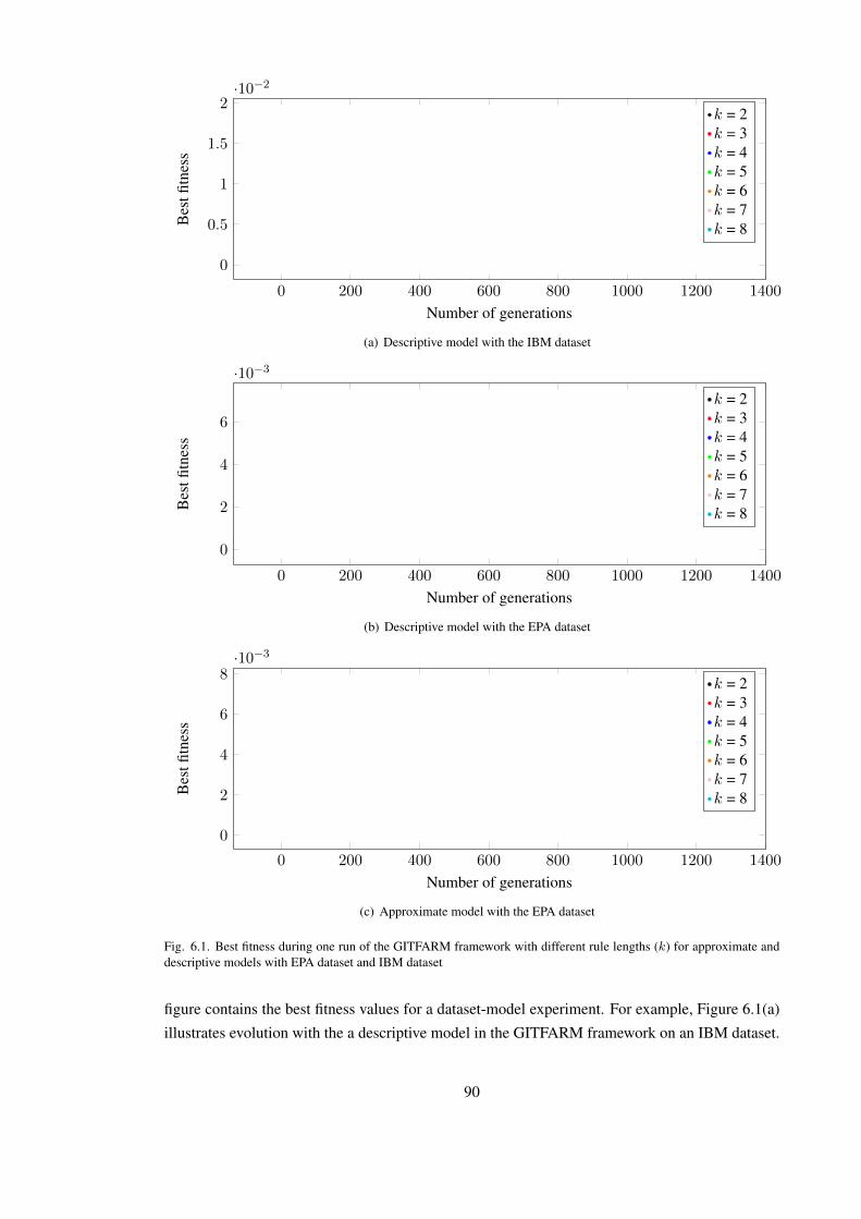
0 200 400 600 800 1000 1200 1400
0
0.5
1
1.5
2·10−2
Number of generations
Bes
tfitn
ess
k = 2k = 3k = 4k = 5k = 6k = 7k = 8
(a) Descriptive model with the IBM dataset
0 200 400 600 800 1000 1200 1400
0
2
4
6
·10−3
Number of generations
Bes
tfitn
ess
k = 2k = 3k = 4k = 5k = 6k = 7k = 8
(b) Descriptive model with the EPA dataset
0 200 400 600 800 1000 1200 1400
0
2
4
6
8·10−3
Number of generations
Bes
tfitn
ess
k = 2k = 3k = 4k = 5k = 6k = 7k = 8
(c) Approximate model with the EPA dataset
Fig. 6.1. Best fitness during one run of the GITFARM framework with different rule lengths (k) for approximate anddescriptive models with EPA dataset and IBM dataset
figure contains the best fitness values for a dataset-model experiment. For example, Figure 6.1(a)
illustrates evolution with the a descriptive model in the GITFARM framework on an IBM dataset.
90

0 200 400 600 800 1000 1200 1400
0
0.5
1
1.5
·10−2
Number of generations
Bes
tfitn
ess
k = 2k = 3k = 4k = 5k = 6k = 7k = 8
(d) Approximate model with the IBM dataset
Fig. 6.1. Best fitness during one run of the GITFARM framework with different rule lengths (k) for approximate anddescriptive models with EPA dataset and IBM dataset (cont.)
Each set of coloured points in a figure represents one run of CHC with a rule length set to k. There
were seven different rule lengths so there are seven sets of coloured points.
Each sub-figure in Figure 6.1 shows that the first generation of CHC starts with a low fitness
that increases in subsequent generations. Figure 6.1 demonstrates how the fitness of the best rule in
each generation evolves so that its fitness increases. In early generations the best fitness increases
quickly, in later generations the best fitness changes less frequently. This phenomenon is referred
to as convergence and it occurs when the solutions in a population of a GA move towards the same
solution, or when a near-optimal solution is discovered. It is also possible that the GA has become
stuck in a local optima. It is not possible to identify true optimal solutions because this requires an
exhaustive search of the dataset. The purpose of using a metaheuristic algorithm, such as a GA,
is to search a very large search space that is computationally infeasible with a traditional search
method such as FuzzyApriori.
It can be observed in Figure 6.1 that there are multiple occurrences of large increases in best
fitness over a small number of generations. For example, the rules with length k = 2 increase
near generation 300 in Figure 6.1(a) and near generation 550 in Figure 6.1(d). A large increase in
fitness over a small number of generations is likely to be caused by a change in nominal data (e.g.,
item, linguistic label) rather than an interval data type (e.g., membership function parameters or
lateral displacement).
It can be observed in Figure 6.1 that many iterations in IRL have different numbers of
generations. A restart is performed at the end of a generation and before the next generation. As a
result of a restart, the population changes and so all individuals in the population are evaluated. It
is the number of restart operations that cause the number of generations to differ because CHC’s
termination criteria is the number of evaluations, and not the number of generations. Fewer
generations in a run of CHC shows that CHC has converged more frequently than a run of CHC
that has produced more generations. Each run of CHC has fewer generations when the rule size
increases. This behaviour can be observed in each model-dataset experiment. This is for only one
91
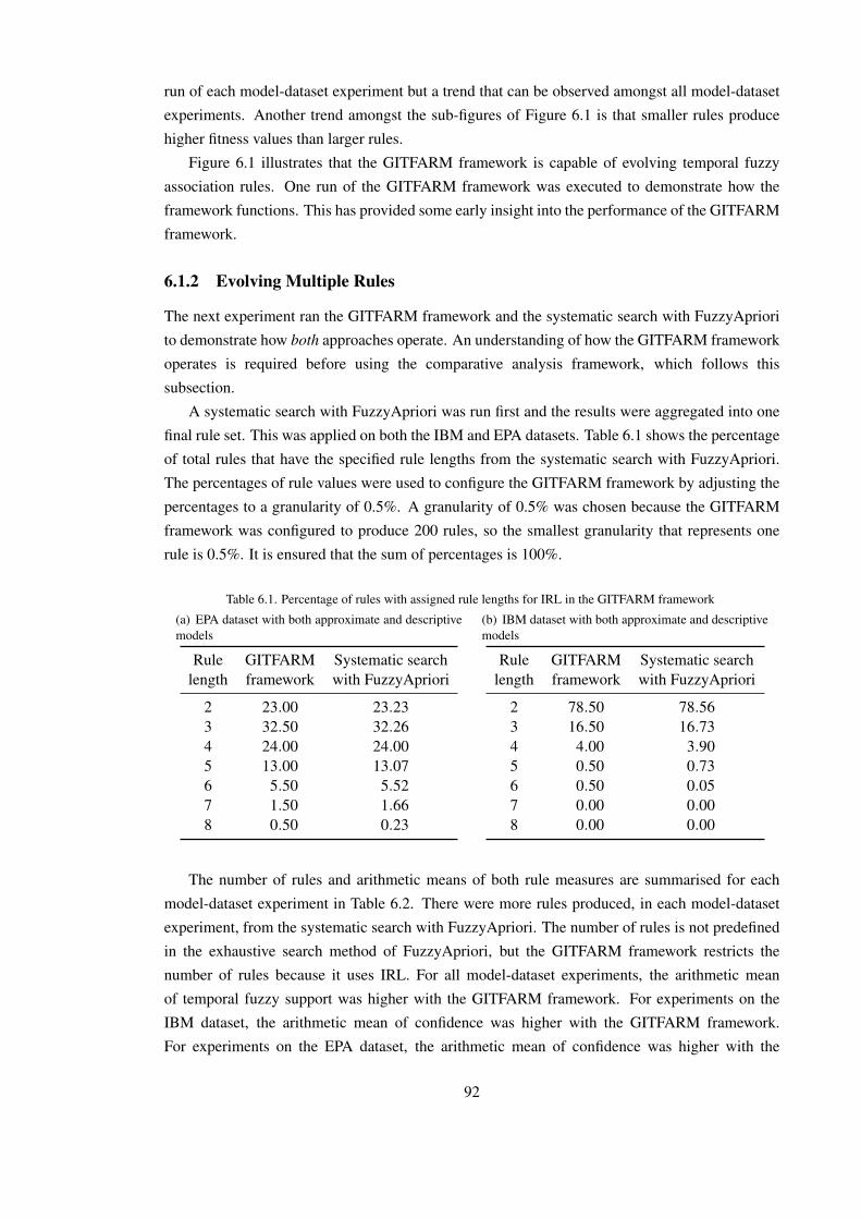
run of each model-dataset experiment but a trend that can be observed amongst all model-dataset
experiments. Another trend amongst the sub-figures of Figure 6.1 is that smaller rules produce
higher fitness values than larger rules.
Figure 6.1 illustrates that the GITFARM framework is capable of evolving temporal fuzzy
association rules. One run of the GITFARM framework was executed to demonstrate how the
framework functions. This has provided some early insight into the performance of the GITFARM
framework.
6.1.2 Evolving Multiple Rules
The next experiment ran the GITFARM framework and the systematic search with FuzzyApriori
to demonstrate how both approaches operate. An understanding of how the GITFARM framework
operates is required before using the comparative analysis framework, which follows this
subsection.
A systematic search with FuzzyApriori was run first and the results were aggregated into one
final rule set. This was applied on both the IBM and EPA datasets. Table 6.1 shows the percentage
of total rules that have the specified rule lengths from the systematic search with FuzzyApriori.
The percentages of rule values were used to configure the GITFARM framework by adjusting the
percentages to a granularity of 0.5%. A granularity of 0.5% was chosen because the GITFARM
framework was configured to produce 200 rules, so the smallest granularity that represents one
rule is 0.5%. It is ensured that the sum of percentages is 100%.
Table 6.1. Percentage of rules with assigned rule lengths for IRL in the GITFARM framework
(a) EPA dataset with both approximate and descriptivemodels
Rule GITFARM Systematic searchlength framework with FuzzyApriori
2 23.00 23.233 32.50 32.264 24.00 24.005 13.00 13.076 5.50 5.527 1.50 1.668 0.50 0.23
(b) IBM dataset with both approximate and descriptivemodels
Rule GITFARM Systematic searchlength framework with FuzzyApriori
2 78.50 78.563 16.50 16.734 4.00 3.905 0.50 0.736 0.50 0.057 0.00 0.008 0.00 0.00
The number of rules and arithmetic means of both rule measures are summarised for each
model-dataset experiment in Table 6.2. There were more rules produced, in each model-dataset
experiment, from the systematic search with FuzzyApriori. The number of rules is not predefined
in the exhaustive search method of FuzzyApriori, but the GITFARM framework restricts the
number of rules because it uses IRL. For all model-dataset experiments, the arithmetic mean
of temporal fuzzy support was higher with the GITFARM framework. For experiments on the
IBM dataset, the arithmetic mean of confidence was higher with the GITFARM framework.
For experiments on the EPA dataset, the arithmetic mean of confidence was higher with the
92

systematic search with FuzzyApriori. These model-dataset experiments are only conducted once
to demonstrate the number of rules and rule measures of each approach.
Table 6.2. Results of approximate/descriptive GITFARM and FuzzyApriori (EPA dataset: 0.0011 minimum temporalfuzzy support and 0.5 confidence. IBM dataset: 0.01 minimum temporal fuzzy support and 0.1 confidence)
(a) Approximate model with the EPA dataset
Measure GITFARM FuzzyApriori
Number of Rules 200 3366Arithmetic mean of temporal fuzzy support (4 d.p.) 0.0026 0.0015Arithmetic mean of confidence (4 d.p.) 0.7854 0.8964
(b) Approximate model with an IBM dataset
Measure GITFARM FuzzyApriori
Number of Rules 200 10234Arithmetic mean of temporal fuzzy support (4 d.p.) 0.0135 0.0108Arithmetic mean of confidence (4 d.p.) 0.9538 0.7616
(c) Descriptive model with the EPA dataset
Measure GITFARM FuzzyApriori
Number of Rules 200 3366Arithmetic mean of temporal fuzzy support (4 d.p.) 0.0020 0.0015Arithmetic mean of confidence (4 d.p.) 0.7783 0.8964
(d) Descriptive model with an IBM dataset
Measure GITFARM FuzzyApriori
Number of Rules 200 10234Arithmetic mean of temporal fuzzy support (4 d.p.) 0.0154 0.0108Arithmetic mean of confidence (4 d.p.) 0.8616 0.7616
Figure 6.2 contains box plots of both rule measures for both the GITFARM framework and the
systematic search with FuzzyApriori for each model-dataset experiment. The box plots illustrate
the distributions of rule measures. The minimum value of a rule produced from the systematic
search with FuzzyApriori is limited to FuzzyApriori’s minimum thresholds. It is not possible for
FuzzyApriori to produce rules that are smaller than the minimum thresholds. The GITFARM
framework does not have this restriction and so rules with lower temporal fuzzy support and
confidence were mined.
The maximum and arithmetic mean temporal fuzzy support was higher in the GITFARM
framework for all model-dataset experiments. This demonstrates that, in these experiments,
the GITFARM framework has produced higher quality rules with respect to temporal fuzzy
support. For confidence, the maximum value was the same in all model-dataset experiments,
but the arithmetic mean was higher with the IBM dataset, which has previously been shown in
Table 6.2. It can be observed that the dispersion of temporal fuzzy support was larger for the
rules produced from the GITFARM framework for all model-dataset experiments. The dispersion
93
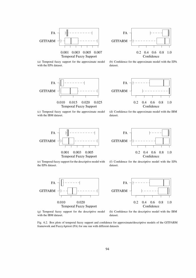
GITFARM
FA
0.001 0.003 0.005 0.007Temporal Fuzzy Support
(a) Temporal fuzzy support for the approximate modelwith the EPA dataset.
GITFARM
FA
0.2 0.4 0.6 0.8 1.0Confidence
(b) Confidence for the approximate model with the EPAdataset.
GITFARM
FA
0.010 0.015 0.020 0.025Temporal Fuzzy Support
(c) Temporal fuzzy support for the approximate modelwith the IBM dataset.
GITFARM
FA
0.2 0.4 0.6 0.8 1.0Confidence
(d) Confidence for the approximate model with the IBMdataset.
GITFARM
FA
0.001 0.003 0.005Temporal Fuzzy Support
(e) Temporal fuzzy support for the descriptive model withthe EPA dataset.
GITFARM
FA
0.2 0.4 0.6 0.8 1.0Confidence
(f) Confidence for the descriptive model with the EPAdataset.
GITFARM
FA
0.010 0.020Temporal Fuzzy Support
(g) Temporal fuzzy support for the descriptive modelwith the IBM dataset.
GITFARM
FA
0.2 0.4 0.6 0.8 1.0Confidence
(h) Confidence for the descriptive model with the IBMdataset.
Fig. 6.2. Box plots of temporal fuzzy support and confidence for approximate/descriptive models of the GITFARMframework and FuzzyApriori (FA) for one run with different datasets
94

of confidence was also larger for the rules produced from the GITFARM framework for the
EPA dataset. Furthermore, the arithmetic mean of confidence for the rules produced from the
GITFARM framework was lower for the EPA dataset. A lower arithmetic mean of confidence
on the EPA dataset may suggest the GITFARM framework has weaker performance on the EPA
dataset with respect to confidence. The opposite is observed with the IBM dataset where the
dispersion of confidence is smaller and the arithmetic mean of confidence is higher.
6.2 Comparative Analysis
The GITFARM framework has been presented and its operation has been demonstrated in the
previous section. The GITFARM framework learns fuzzy association rules that have an intra-
transaction temporal pattern. The purpose of the GITFARM framework is to discover rules that
a traditional approach (FuzzyApriori) cannot. The previous section demonstrated preliminary
results with the approximate and descriptive models of the GITFARM framework on two datasets.
It is now understood that the GITFARM framework is capable of evolving rules. Experiments in
this section now focus on the hypothesis, which was defined in Section 1.2.
All runs of the GITFARM framework were repeated 30 times for all experiments. The same
two datasets used in the previous section were used in these experiments.
The previous model-dataset experiments, from Section 6.1.1, were used again. There were
four sets of experiments with different combinations of dataset and model. The percentage of
rules with assigned rule lengths for IRL in the GITFARM framework were assigned the same
values as in the previous section, i.e., Table 6.1.
The rules were analysed in the comparative analysis framework and are presented in Table 6.3.
The percentages refers to the ratio of rules discovered with the GITFARM framework, i.e., the
percentage of 200 rules. The terms describing the rows are:
GITFARM and FA The percentage of rules from the GITFARM framework that matched the
rules discovered with FuzzyApriori. These are considered to be existing rules.
GITFARM only The percentage of rules from the GITFARM framework that did not match the
rules discovered with FuzzyApriori. These are considered to be new rules, or rules that have
been lost with FuzzyApriori.
Rules discovered by both approaches are discussed first, i.e., percentages described as
GITFARM and FA. The change in temporal fuzzy support and confidence for those rules was
analysed to determine increases, decreases and no changes. By analysing the change in values for
both metrics more information can be deduced about the behaviour of the GITFARM framework.
Rules are said to be improved by the GITFARM framework when two conditions are met: a) rule
discovered with both methods; and b) the change in metric is an increase. So, 39.13% and 33.62%
of rules had increases in temporal fuzzy support and confidence respectively, for an approximate
model with the EPA dataset. 36.60% and 31.40% of rules had increases in temporal fuzzy support
and confidence respectively, for an approximate model with the IBM dataset. 46.03% and 32.75%
95

of rules had increases in temporal fuzzy support and confidence respectively, for a descriptive
model with the EPA dataset. 56.12% and 45.78% of rules had increases in temporal fuzzy support
and confidence respectively, for a descriptive model with the IBM dataset. It can be observed that
the descriptive approach had more improved rules with both datasets except the confidence with
the EPA dataset. A possible reason for this is the search space size is smaller with a descriptive
model because the membership function parameters are represented with only one real-value
parameter, whilst there are three real-value parameters in the approximate model.
It has been demonstrated how the GITFARM framework produces rules that are an
improvement over the rules produced with FuzzyApriori. The hypothesis of this thesis focuses
on exploring a method for discovering rules that a traditional approach cannot. Table 6.3 also
presents the total number of rules that were only discovered with the GITFARM framework. There
were 54.87% of rules only discovered with the GITFARM framework for an approximate model
with the EPA dataset, 61.40% with the approximate and IBM dataset, 53.40% with the descriptive
dataset and 40.53% with the descriptive and IBM dataset. These figures show rules that were only
discovered with the GITFARM framework. For example, 54.87% of 200 rules is 109.74 rules,
which is the arithmetic mean of 30 runs. Further analysis is required to identify why these rules
are not present in the results of FuzzyApriori, i.e., why the rules were lost.
An analysis of why the rules are only discovered with the GITFARM framework, and not
FuzzyApriori, is presented in Table 6.4. Table 6.4 provides a more detailed analysis of the data
from Table 6.3. For example, Table 6.3(a) shows a total of 54.87% rules were only discovered
with the GITFARM framework, Table 6.4(a) analyses those 54.87% of rules to discover why they
were lost for that particular model-dataset experiment. The terms describing the columns are:
Discarded by threshold(s) Rules not discovered with FuzzyApriori because of one or more
minimum thresholds.
Above threshold(s) Rules not discovered with FuzzyApriori that are now greater than or equal
to both minimum thresholds. These are referred to as lost rules.
Rules were discarded with FuzzyApriori because rules were below the minimum temporal
fuzzy support threshold, the minimum confidence threshold, or both minimum thresholds.
The traditional approach discarded rules, but when the GITFARM framework discovers those
discarded rules, they are referred to as new rules. When the new rules are greater than or equal to
the minimum thresholds, they are referred to as lost rules.
The largest cause of rules being discarded by FuzzyApriori was the temporal fuzzy support
threshold in all model-dataset experiments. This observation could suggest that minimum
temporal fuzzy support is an influential factor in discovering rules. Temporal fuzzy support and
confidence were factors in losing rules with the EPA dataset. Temporal fuzzy support was a factor
in losing rules with the IBM dataset and confidence only lost a small percentage (0.01%) for the
descriptive model. More lost rules were discovered with the IBM dataset than the EPA dataset.
Having analysed why rules were lost, it is important to identify the GITFARM framework’s
ability in discovering rules that are now greater than or equal to the minimum thresholds. This
96

Table 6.3. Analysis of temporal fuzzy support and confidence for rules discovered with the approximate and descriptivemodels of GITFARM framework and the systematic search with FuzzyApriori (FA)
(a) Temporal fuzzy support and confidence for approximate model and EPA dataset
Arithmetic mean of change in Arithmetic mean of change inTemporal Fuzzy Support (%) Confidence (%)
-ve 0 +ve Total -ve 0 +ve Total
GITFARM and FA 6.00 0.00 39.13 45.13 5.47 6.05 33.62 45.13GITFARM only 1.35 4.80 48.72 54.87 2.65 36.63 15.58 54.87
(b) Temporal fuzzy support and confidence for approximate model and IBM dataset
Arithmetic mean of change in Arithmetic mean of change inTemporal Fuzzy Support (%) Confidence (%)
-ve 0 +ve Total -ve 0 +ve Total
GITFARM and FA 2.00 0.00 36.60 38.60 4.00 3.20 31.40 38.60GITFARM only 0.00 0.00 61.40 61.40 5.30 24.30 31.80 61.40
(c) Temporal fuzzy support and confidence for descriptive model and EPA dataset
Arithmetic mean of change in Arithmetic mean of change inTemporal Fuzzy Support (%) Confidence (%)
-ve 0 +ve Total -ve 0 +ve Total
GITFARM and FA 0.57 0.00 46.03 46.60 6.97 6.88 32.75 46.60GITFARM only 0.55 0.23 52.62 53.40 4.00 30.15 19.25 53.40
(d) Temporal fuzzy support and confidence for descriptive model and IBM dataset
Arithmetic mean of change in Arithmetic mean of change inTemporal Fuzzy Support (%) Confidence (%)
-ve 0 +ve Total -ve 0 +ve Total
GITFARM and FA 0.23 3.12 56.12 59.47 9.82 3.87 45.78 59.47GITFARM only 0.00 0.00 40.53 40.53 7.97 15.73 16.83 40.53
will support the verification of the hypothesis. Since the thresholds are determined by the user
as levels of significance for rules, only rules that have evolved to be greater than or equal to the
minimum temporal fuzzy support threshold are of interest. Table 6.4 shows the percentage of rules
discovered only by the GITFARM framework that are now greater than or equal to the minimum
thresholds. It can be observed that all model-dataset experiments produced rules with measures
that are greater than or equal to one or both minimum thresholds. It is these rules, which are now
greater than or equal to the minimum thresholds, that are considered to be the lost rules that are
only discovered with the GITFARM framework. Without the GITFARM framework, these rules
97

Table 6.4. Rules discovered with the approximate and descriptive models of GITFARM framework that were lost andare now greater than or equal to the threshold(s)The EPA dataset was preprocessed with a 10 minute time windowfor forward reference model. The IBM dataset was generated with 10000 transactions, 1000 items and a maximumquantitative value of 20.
(a) Approximate model and EPA dataset
Discarded by Greater than or equal tothreshold(s) (%) threshold(s) (%)
Below min. temporal fuzzy support only 43.07 3.35Below min. confidence only 6.53 1.05Below both (greater than or equal to both) 5.27 0.05
Total 54.87 4.45
(b) Approximate model and IBM dataset
Discarded by Greater than or equal tothreshold(s) (%) threshold(s) (%)
Below min. temporal fuzzy support only 61.40 11.65Below min. confidence only 0.00 0.00Below both (greater than or equal to both) 0.00 0.00
Total 61.40 11.65
(c) Descriptive model and EPA dataset
Discarded by Greater than or equal tothreshold(s) (%) threshold(s) (%)
Below min. temporal fuzzy support only 42.02 6.03Below min. confidence only 8.60 2.07Below both (greater than or equal to both) 2.78 1.98
Total 53.40 10.08
(d) Descriptive model and IBM dataset
Discarded by Greater than or equal tothreshold(s) (%) threshold(s) (%)
Below min. temporal fuzzy support only 40.52 17.67Below min. confidence only 0.00 0.00Below both (greater than or equal to both) 0.01 0.01
Total 40.53 17.68
would not have been discovered. However, as previously stated, lowering the minimum threshold
values would allow FuzzyApriori to discover these rules, but at the cost of discovering many more
rules because of combinatorial explosion.
In Table 6.4, it can be observed that when rules were below one or both thresholds, a
98

proportion of those rules were improved so they are greater than or equal to the threshold. This
is observed for all model-dataset experiments. For example, for the approximate model and the
EPA dataset (Table 6.4), 43.07% were discarded by FuzzyApriori and 3.35% were discovered with
the GITFARM framework. Note that both 43.07% and 3.35% are both percentages of 200 rules.
Table 6.4 does not show rules that were below one threshold and greater than or equal to another
threshold because rules must be greater than or equal to both thresholds.
Results have been presented and analysed to ascertain how the GITFARM framework
discovers new rules. Some of the new rules are considered to have been lost by FuzzyApriori. A
single rule from each model-dataset experiment is presented below for a new rule. All values for
membership function parameters and lateral displacement are rounded to two significant figures.
Note that each rule is now greater than or equal to both minimum thresholds. Each rule was taken
from the results of the first run of 30 runs.
Endpoints: 30th August 1995 14:00:00 EDT – 30th August 1995 15:00:00 EDT
Rule: IF page view time of /docs/Welcome is approximately 15.89 seconds
Rule: (membership function parameters: 6.16, 15.89, 243.20)
Rule: THEN page view time of /Rules.html is approximately 6.05 seconds
Rule: (membership function parameters: -209.10, 6.05, 292.97)
Temporal Fuzzy Support: 0.0017
Confidence: 1.0
Approximate model and IBM dataset:
Endpoints: 7700–7800
Rule: IF quantity of Item467 is approximately 1.40
Rule: (membership function parameters: -7.81, 1.40, 10.89)
Rule: THEN quantity of Item540 is approximately 16.32
Rule: (membership function parameters: 7.52, 16.32, 20.65)
Temporal Fuzzy Support: 0.019
Confidence: 1.0
Descriptive model and EPA dataset:
Endpoints: 30th August 1995 14:00:00 EDT – 30th August 1995 15:00:00 EDT
Rule: IF page view time of /EPA-AIR/ is (medium, -0.49)
Rule: AND page view time of /docs/EPA-AIR is (medium, -0.49)
Rule: THEN page view time of /Rules.html is (low, 0.30)
Temporal Fuzzy Support: 0.0018
Confidence: 1.0
Descriptive model and IBM dataset:
Endpoints: 5200–5300
Rule: IF quantity of Item64 is (medium, 0.28)
Rule: THEN quantity of Item368 is (high, -0.50)
99
Temporal Fuzzy Support: 0.017
Confidence: 0.97
It has been demonstrated how the GITFARM framework can discover rules that a traditional
approach (FuzzyApriori) cannot. Different models of the GITFARM framework have been applied
on two different datasets.
6.3 Varying the Number of Membership Functions
Creating more membership functions can provide a finer level of granularity for covering the
universe of discourse. If rules are lost because the patterns occur at the intersection of membership
functions then it could be perceived as logical to create more membership functions to cover
those intersections. Creating more membership functions is a possible solution to the problem
that this thesis tackles. However, increasing the number of linguistic labels used to describe the
membership functions can decrease the interpretability of rules (Ishibuchi and Nojima, 2009).
Experiments were conducted to assess how the number of membership functions affects the
number of temporal fuzzy associations rules that have previously been shown to be lost in this
thesis. The comparative analysis framework is utilised again.
Experiments were conducted on the same datasets used in Section 6.2, there are four model-
dataset experiments that combine approximate/descriptive models and the IBM/EPA dataset. The
approximate models of the GITFARM framework use fuzzy numbers without linguistic terms.
Increasing the number of membership functions is not applicable to the approximate model of the
GITFARM framework. The number of membership functions is relevant to FuzzyApriori because
linguistic terms are used.
The FuzzyApriori approach was run with different numbers of membership functions. The
number of rules discovered is presented in Table 6.5. The configuration for the number of
rules with different rule lengths was determined from the results of FuzzyApriori and set to the
percentage values in Table 6.6. The width of membership functions (distance between parameters
a and c in a triangular membership function) in an approximate model is important for a fair
comparison with FuzzyApriori, which has been discussed in Section 5.2.6. The width parameter
in the approximate model is configured to be the same as the width of the uniform membership
functions in FuzzyApriori. To illustrate this, Table 6.7 presents the width parameters used for an
approximate model of the GITFARM framework with both the EPA and an IBM dataset.
Figure 6.3 presents the results of comparing the rules from both approaches. Each bar
represents a percentage of rules discovered with the GITFARM set to 200 iterations of IRL. The
terms describing the keys are the same as those used previously in Section 6.2 on page 95.
It can be observed in Figure 6.3 that the GITFARM framework discovers more rules, and
FuzzyApriori discovers fewer rules, as the number of membership functions increases for all
model-dataset experiments. As the number of membership functions increases with the IBM
datasets, the number of rules only discovered with the GITFARM framework increases.
Figure 6.4 shows the percentage of rules now greater than or equal to the temporal fuzzy
100

Table 6.5. Number of rules found in FuzzyApriori when using different numbers of membership functions
(a) The EPA dataset
Number of membership functions Number of rules
3 33665 25917 22489 1964
(b) The IBM dataset
Number of membership functions Number of rules
3 102345 76057 71029 6780
Table 6.6. Percentage of rules with assigned rule lengths for IRL with different numbers of membership functions
(a) The EPA dataset
Number of membership functions
Rule length 3 5 7 9
2 23.0 24.0 23.5 24.03 32.5 31.0 30.0 28.04 24.0 22.5 22.0 21.05 13.0 13.5 14.0 15.06 5.5 6.5 7.5 8.57 1.5 2.0 2.5 3.08 0.5 0.5 0.5 0.5
(b) The IBM dataset
Number of membership functions
Rule length 3 5 7 9
2 78.5 72.5 71.0 69.53 16.5 21.0 22.5 23.04 4.0 5.0 5.5 6.05 0.5 1.0 0.5 1.06 0.5 0.5 0.5 0.57 0.0 0.0 0.0 0.08 0.0 0.0 0.0 0.0
support threshold. The results in Figure 6.4 are a subset of the rules only discovered with the
GITFARM framework. The total number of rules now greater than or equal to the minimum
thresholds increases with the number of membership functions in the approximate model and
101
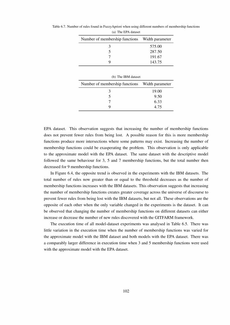
Table 6.7. Number of rules found in FuzzyApriori when using different numbers of membership functions
(a) The EPA dataset
Number of membership functions Width parameter
3 575.005 287.507 191.679 143.75
(b) The IBM dataset
Number of membership functions Width parameter
3 19.005 9.507 6.339 4.75
EPA dataset. This observation suggests that increasing the number of membership functions
does not prevent fewer rules from being lost. A possible reason for this is more membership
functions produce more intersections where some patterns may exist. Increasing the number of
membership functions could be exasperating the problem. This observation is only applicable
to the approximate model with the EPA dataset. The same dataset with the descriptive model
followed the same behaviour for 3, 5 and 7 membership functions, but the total number then
decreased for 9 membership functions.
In Figure 6.4, the opposite trend is observed in the experiments with the IBM datasets. The
total number of rules now greater than or equal to the threshold decreases as the number of
membership functions increases with the IBM datasets. This observation suggests that increasing
the number of membership functions creates greater coverage across the universe of discourse to
prevent fewer rules from being lost with the IBM datasets, but not all. These observations are the
opposite of each other when the only variable changed in the experiments is the dataset. It can
be observed that changing the number of membership functions on different datasets can either
increase or decrease the number of new rules discovered with the GITFARM framework.
The execution time of all model-dataset experiments was analysed in Table 6.5. There was
little variation in the execution time when the number of membership functions was varied for
the approximate model with the IBM dataset and both models with the EPA dataset. There was
a comparably larger difference in execution time when 3 and 5 membership functions were used
with the approximate model with the EPA dataset.
102

3 5 7 90
20
40
60
80
100
Number of membership functions
Rul
esfr
omG
ITFA
RM
(%)
Rules in GITFARM onlyRules in GITFARM and FA
(a) Approximate model with EPA dataset
3 5 7 90
20
40
60
80
100
Number of membership functionsR
ules
from
GIT
FAR
M(%
)
Rules in GITFARM onlyRules in GITFARM and FA
(b) Approximate model with IBM dataset
3 5 7 90
20
40
60
80
100
Number of membership functions
Rul
esfr
omG
ITFA
RM
(%)
Rules in GITFARM onlyRules in GITFARM and FA
(c) Descriptive model with EPA dataset
3 5 7 90
20
40
60
80
100
Number of membership functions
Rul
esfr
omG
ITFA
RM
(%)
Rules in GITFARM onlyRules in GITFARM and FA
(d) Descriptive model with IBM dataset
Fig. 6.3. Percentage of rules found with only the GITFARM framework and both approaches with different numbersof membership functions
103
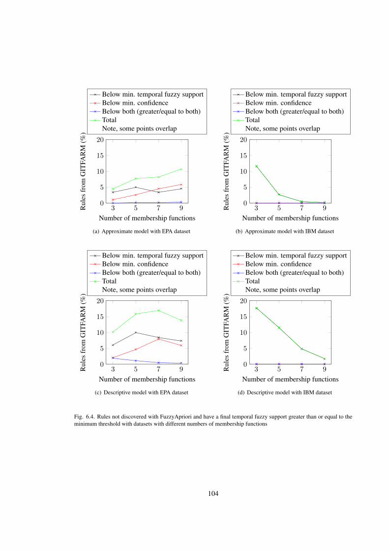
3 5 7 90
5
10
15
20
Number of membership functions
Rul
esfr
omG
ITFA
RM
(%)
Below min. temporal fuzzy supportBelow min. confidenceBelow both (greater/equal to both)TotalNote, some points overlap
(a) Approximate model with EPA dataset
3 5 7 90
5
10
15
20
Number of membership functionsR
ules
from
GIT
FAR
M(%
)
Below min. temporal fuzzy supportBelow min. confidenceBelow both (greater/equal to both)TotalNote, some points overlap
(b) Approximate model with IBM dataset
3 5 7 90
5
10
15
20
Number of membership functions
Rul
esfr
omG
ITFA
RM
(%)
Below min. temporal fuzzy supportBelow min. confidenceBelow both (greater/equal to both)TotalNote, some points overlap
(c) Descriptive model with EPA dataset
3 5 7 90
5
10
15
20
Number of membership functions
Rul
esfr
omG
ITFA
RM
(%)
Below min. temporal fuzzy supportBelow min. confidenceBelow both (greater/equal to both)TotalNote, some points overlap
(d) Descriptive model with IBM dataset
Fig. 6.4. Rules not discovered with FuzzyApriori and have a final temporal fuzzy support greater than or equal to theminimum threshold with datasets with different numbers of membership functions
104
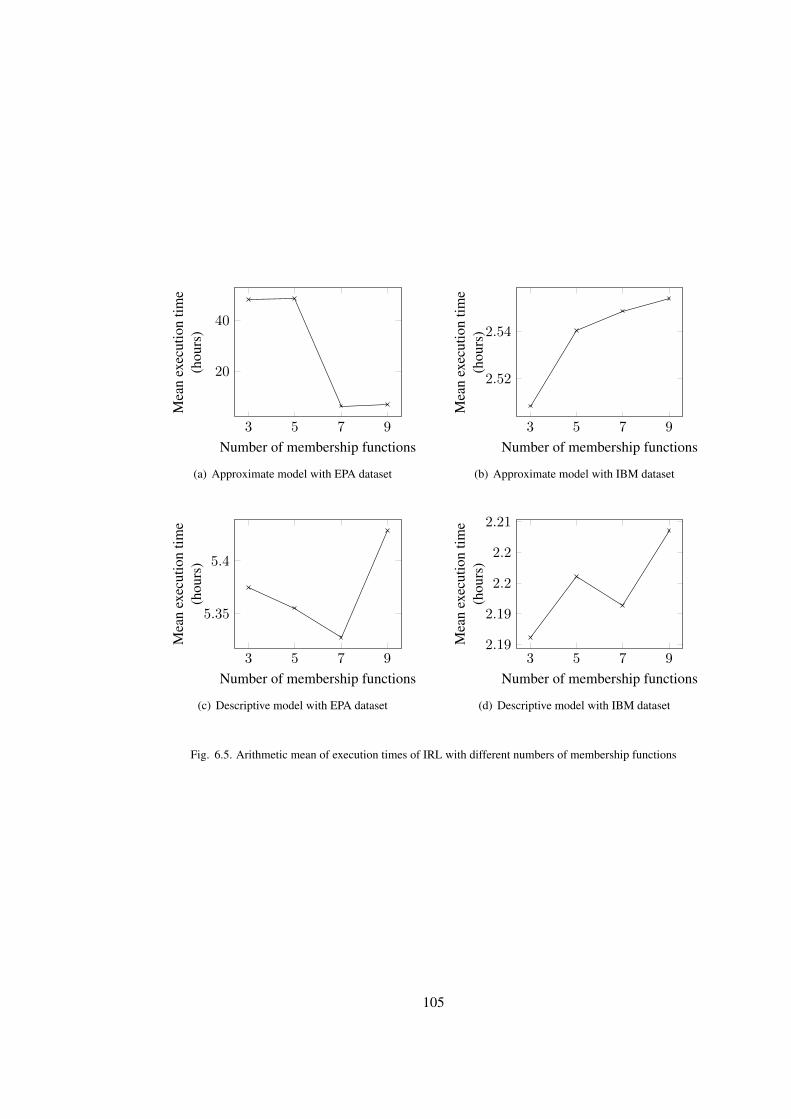
3 5 7 9
20
40
Number of membership functions
Mea
nex
ecut
ion
time
(hou
rs)
(a) Approximate model with EPA dataset
3 5 7 9
2.52
2.54
Number of membership functionsM
ean
exec
utio
ntim
e(h
ours
)(b) Approximate model with IBM dataset
3 5 7 9
5.35
5.4
Number of membership functions
Mea
nex
ecut
ion
time
(hou
rs)
(c) Descriptive model with EPA dataset
3 5 7 92.19
2.19
2.2
2.2
2.21
Number of membership functions
Mea
nex
ecut
ion
time
(hou
rs)
(d) Descriptive model with IBM dataset
Fig. 6.5. Arithmetic mean of execution times of IRL with different numbers of membership functions
105

6.4 Analysis of Number of Transactions
To assess the scalability of the GITFARM framework, the number of transactions in the synthetic
datasets was varied. Previous experiments were limited to 2687 transactions in the EPA dataset
and 10000 transactions with the synthetic dataset. In these experiments, generation of the synthetic
dataset was varied to produce datasets with 10000, 30000, 50000, 70000 and 90000 transactions.
The traditional approach, FuzzyApriori, was run on the five synthetic datasets that have
different numbers of transactions. Table 6.8 shows the number of rules in IRL assigned to
different rule lengths for each dataset. Table 6.9 shows the number of rules discovered with
the FuzzyApriori approach. Two sets of experiments were conducted: different sized synthetic
datasets with the approximate model of GITFARM framework and different sized synthetic
datasets with the descriptive model of GITFARM framework.
Table 6.8. Percentage of rules with assigned rule lengths for IRL on datasets with varying numbers of transactions
Number of transactions
Rule length 10000 30000 50000 70000 90000
2 78.5 80.0 79.5 79.5 80.03 16.5 16.0 16.0 16.0 15.54 4.0 3.0 3.5 3.5 3.55 0.5 0.5 0.5 0.5 0.56 0.5 0.5 0.5 0.5 0.5
Table 6.9. Number of rules discovered in FuzzyApriori
Number of transactions in dataset Number of rules
10000 1023430000 3049250000 5087570000 7118290000 91135
It can be observed from Figure 6.6 that the number of rules only discovered with the
GITFARM framework increases with the number of transactions for the descriptive model. The
same observation cannot be made for the approximate model; there is no increase in the number of
rules that correlates with the number of transactions. This means that the GITFARM framework
is capable of discovering a larger proportion of rules with a descriptive model when the number of
transactions increase, but the same proportion of rules for the approximate model.
New rules from the GITFARM framework, which are now greater than or equal to the
minimum thresholds, are presented in Figure 6.7. It can be observed that both the approximate and
descriptive models have similar behaviour when increasing the number of transactions. The total
number of rules discovered that are now greater than or equal to the minimum thresholds does
not change when the number of transactions increase. This is the same observation made for the
proportion of rules only discovered with the GITFARM framework for the approximate model,
106

10000
30000
50000
70000
90000
0
20
40
60
80
100
Number of transactions
Rul
esfr
omG
ITFA
RM
(%)
Rules in GITFARM onlyRules in GITFARM and FA
(a) Approximate model and IBM datasets
10000
30000
50000
70000
90000
0
20
40
60
80
100
Number of transactions
Rul
esfr
omG
ITFA
RM
(%)
Rules in GITFARM onlyRules in GITFARM and FA
(b) Descriptive model and IBM datasets
Fig. 6.6. Arithmetic mean of percentage of rules discovered with the GITFARM framework and FuzzyApriori, andGITFARM framework for datasets with different numbers of transactions
i.e., Figure 6.6(a). However, a trend was observed in the proportion of rules only discovered
with the GITFARM framework for the descriptive model, i.e., Figure 6.6(b). Despite there
being an apparent relationship between the number of transactions and the percentage of rules
only discovered with the GITFARM framework in Figure 6.6(b), there does not appear to be a
relationship for rules that are now greater than or equal to the minimum temporal fuzzy support
threshold in Figure 6.7(b).
10000
30000
50000
70000
90000
0
10
20
Number of transactions
Rul
esfr
omG
ITFA
RM
(%)
Below min. temporal fuzzy supportBelow min. confidenceBelow bothTotalNote, – overlaps – , and – overlaps –
(a) Approximate model and IBM datasets
10000
30000
50000
70000
90000
0
10
20
Number of transactions
Rul
esfr
omG
ITFA
RM
(%)
Below min. temporal fuzzy supportBelow min. confidenceBelow bothTotalNote, – overlaps – , and – overlaps –
(b) Descriptive model and IBM datasets
Fig. 6.7. Arithmetic mean of rules not discovered in FuzzyApriori and now have measures greater than or equal to oneor both minimum thresholds for datasets with different numbers of transactions
Figure 6.8 illustrates that the execution time appears to scale linearly with the number of
107
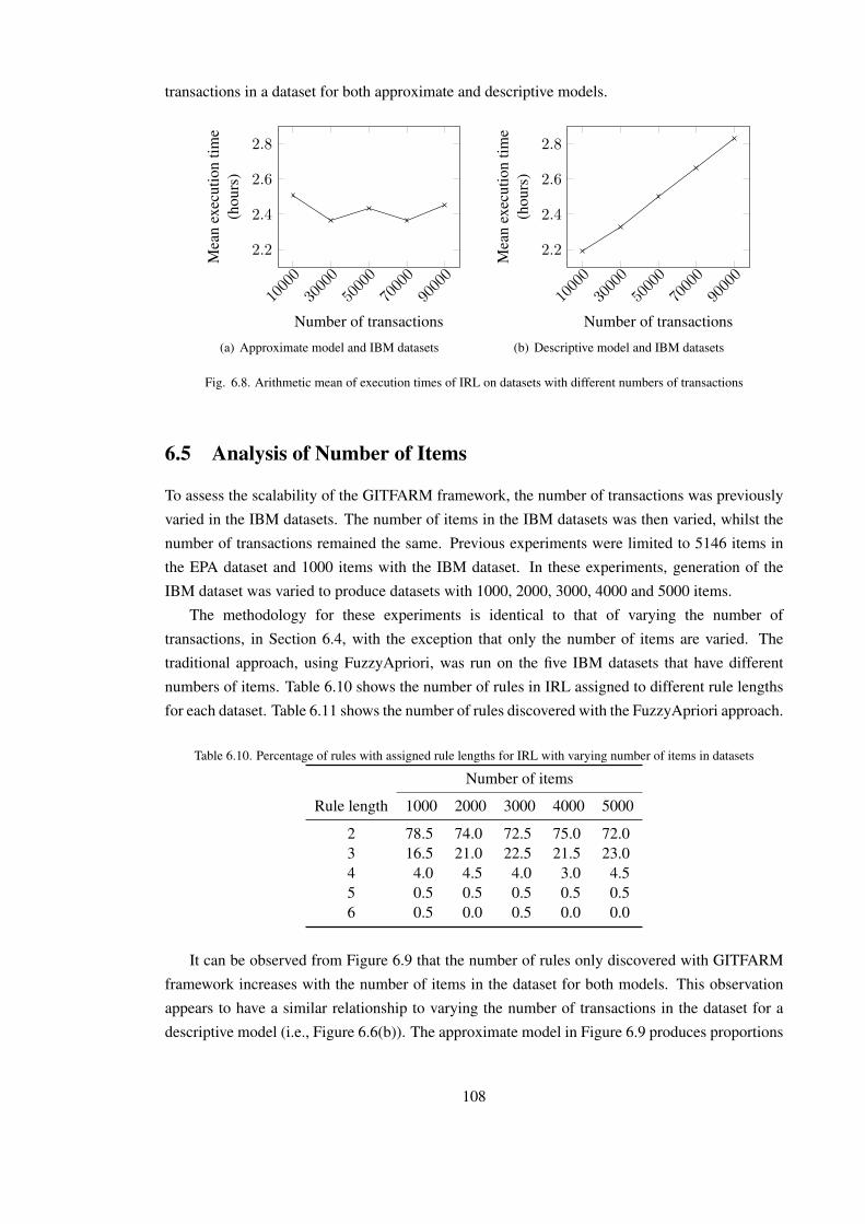
transactions in a dataset for both approximate and descriptive models.
10000
30000
50000
70000
90000
2.2
2.4
2.6
2.8
Number of transactions
Mea
nex
ecut
ion
time
(hou
rs)
(a) Approximate model and IBM datasets
10000
30000
50000
70000
90000
2.2
2.4
2.6
2.8
Number of transactions
Mea
nex
ecut
ion
time
(hou
rs)
(b) Descriptive model and IBM datasets
Fig. 6.8. Arithmetic mean of execution times of IRL on datasets with different numbers of transactions
6.5 Analysis of Number of Items
To assess the scalability of the GITFARM framework, the number of transactions was previously
varied in the IBM datasets. The number of items in the IBM datasets was then varied, whilst the
number of transactions remained the same. Previous experiments were limited to 5146 items in
the EPA dataset and 1000 items with the IBM dataset. In these experiments, generation of the
IBM dataset was varied to produce datasets with 1000, 2000, 3000, 4000 and 5000 items.
The methodology for these experiments is identical to that of varying the number of
transactions, in Section 6.4, with the exception that only the number of items are varied. The
traditional approach, using FuzzyApriori, was run on the five IBM datasets that have different
numbers of items. Table 6.10 shows the number of rules in IRL assigned to different rule lengths
for each dataset. Table 6.11 shows the number of rules discovered with the FuzzyApriori approach.
Table 6.10. Percentage of rules with assigned rule lengths for IRL with varying number of items in datasets
Number of items
Rule length 1000 2000 3000 4000 5000
2 78.5 74.0 72.5 75.0 72.03 16.5 21.0 22.5 21.5 23.04 4.0 4.5 4.0 3.0 4.55 0.5 0.5 0.5 0.5 0.56 0.5 0.0 0.5 0.0 0.0
It can be observed from Figure 6.9 that the number of rules only discovered with GITFARM
framework increases with the number of items in the dataset for both models. This observation
appears to have a similar relationship to varying the number of transactions in the dataset for a
descriptive model (i.e., Figure 6.6(b)). The approximate model in Figure 6.9 produces proportions
108

Table 6.11. Number of rules found in FuzzyApriori with varying number of items in datasets
Number of items Number of rules
1000 102342000 73423000 68494000 62615000 6387
of rules only discovered by the GITFARM framework that are smaller than the descriptive model.
This observation suggests that the approximate model performs better in these experiments.
1000 2000 3000 4000 50000
20
40
60
80
100
Number of items
Rul
esfr
omG
ITFA
RM
(%)
Rules in GITFARM onlyRules in GITFARM and FA
(a) Approximate model and IBM datasets
1000 2000 3000 4000 50000
20
40
60
80
100
Number of items
Rul
esfr
omG
ITFA
RM
(%)
Rules in GITFARM onlyRules in GITFARM and FA
(b) Descriptive model and IBM datasets
Fig. 6.9. Percentage of rules found with only the GITFARM framework and both approaches with different numbersof items
New rules from the GITFARM framework, which are now greater than or equal to the
minimum thresholds, are presented in Figure 6.10. It can be observed that the total number of
rules discovered that are now greater than or equal to the minimum thresholds increases for the
approximate model as the number of items increases. For the descriptive model, a decrease is
observed, with the exception of the dataset with 2000 items.
From observing the arithmetic mean of execution times in Figure 6.11 there is a relationship
between execution time and the number of items in a dataset for the approximate model. For
the descriptive model, there is not such a clear relationship. However, the arithmetic mean of
execution times for datasets with 4000 and 5000 items are higher than those for the other datasets
with 1000, 2000 and 3000 items.
109
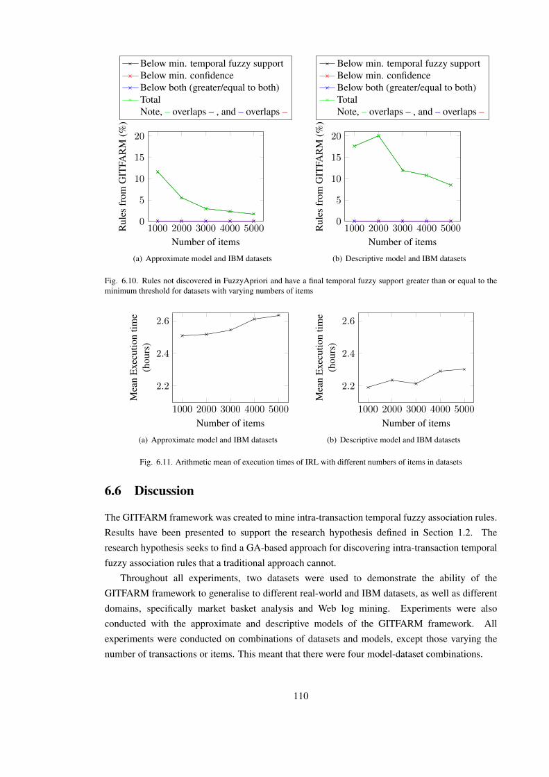
1000 2000 3000 4000 50000
5
10
15
20
Number of items
Rul
esfr
omG
ITFA
RM
(%)
Below min. temporal fuzzy supportBelow min. confidenceBelow both (greater/equal to both)TotalNote, – overlaps – , and – overlaps –
(a) Approximate model and IBM datasets
1000 2000 3000 4000 50000
5
10
15
20
Number of items
Rul
esfr
omG
ITFA
RM
(%)
Below min. temporal fuzzy supportBelow min. confidenceBelow both (greater/equal to both)TotalNote, – overlaps – , and – overlaps –
(b) Descriptive model and IBM datasets
Fig. 6.10. Rules not discovered in FuzzyApriori and have a final temporal fuzzy support greater than or equal to theminimum threshold for datasets with varying numbers of items
1000 2000 3000 4000 5000
2.2
2.4
2.6
Number of items
Mea
nE
xecu
tion
time
(hou
rs)
(a) Approximate model and IBM datasets
1000 2000 3000 4000 5000
2.2
2.4
2.6
Number of items
Mea
nE
xecu
tion
time
(hou
rs)
(b) Descriptive model and IBM datasets
Fig. 6.11. Arithmetic mean of execution times of IRL with different numbers of items in datasets
6.6 Discussion
The GITFARM framework was created to mine intra-transaction temporal fuzzy association rules.
Results have been presented to support the research hypothesis defined in Section 1.2. The
research hypothesis seeks to find a GA-based approach for discovering intra-transaction temporal
fuzzy association rules that a traditional approach cannot.
Throughout all experiments, two datasets were used to demonstrate the ability of the
GITFARM framework to generalise to different real-world and IBM datasets, as well as different
domains, specifically market basket analysis and Web log mining. Experiments were also
conducted with the approximate and descriptive models of the GITFARM framework. All
experiments were conducted on combinations of datasets and models, except those varying the
number of transactions or items. This meant that there were four model-dataset combinations.
110
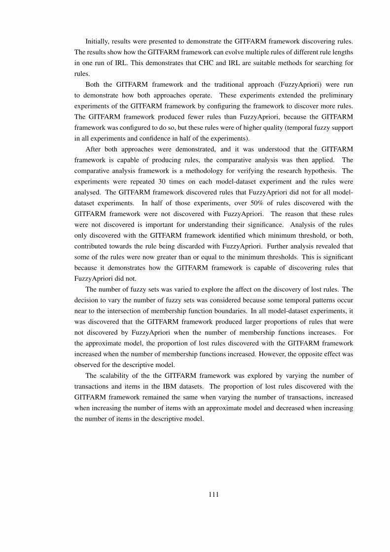
Initially, results were presented to demonstrate the GITFARM framework discovering rules.
The results show how the GITFARM framework can evolve multiple rules of different rule lengths
in one run of IRL. This demonstrates that CHC and IRL are suitable methods for searching for
rules.
Both the GITFARM framework and the traditional approach (FuzzyApriori) were run
to demonstrate how both approaches operate. These experiments extended the preliminary
experiments of the GITFARM framework by configuring the framework to discover more rules.
The GITFARM framework produced fewer rules than FuzzyApriori, because the GITFARM
framework was configured to do so, but these rules were of higher quality (temporal fuzzy support
in all experiments and confidence in half of the experiments).
After both approaches were demonstrated, and it was understood that the GITFARM
framework is capable of producing rules, the comparative analysis was then applied. The
comparative analysis framework is a methodology for verifying the research hypothesis. The
experiments were repeated 30 times on each model-dataset experiment and the rules were
analysed. The GITFARM framework discovered rules that FuzzyApriori did not for all model-
dataset experiments. In half of those experiments, over 50% of rules discovered with the
GITFARM framework were not discovered with FuzzyApriori. The reason that these rules
were not discovered is important for understanding their significance. Analysis of the rules
only discovered with the GITFARM framework identified which minimum threshold, or both,
contributed towards the rule being discarded with FuzzyApriori. Further analysis revealed that
some of the rules were now greater than or equal to the minimum thresholds. This is significant
because it demonstrates how the GITFARM framework is capable of discovering rules that
FuzzyApriori did not.
The number of fuzzy sets was varied to explore the affect on the discovery of lost rules. The
decision to vary the number of fuzzy sets was considered because some temporal patterns occur
near to the intersection of membership function boundaries. In all model-dataset experiments, it
was discovered that the GITFARM framework produced larger proportions of rules that were
not discovered by FuzzyApriori when the number of membership functions increases. For
the approximate model, the proportion of lost rules discovered with the GITFARM framework
increased when the number of membership functions increased. However, the opposite effect was
observed for the descriptive model.
The scalability of the the GITFARM framework was explored by varying the number of
transactions and items in the IBM datasets. The proportion of lost rules discovered with the
GITFARM framework remained the same when varying the number of transactions, increased
when increasing the number of items with an approximate model and decreased when increasing
the number of items in the descriptive model.
111

Chapter 7
Conclusions
The conclusions draw an end to this thesis. A brief summary of the main points is presented
in Section 7.1. Conclusions and research contributions for the entire thesis are examined in
Section 7.2. Considerations for further work are discussed in Section 7.3.
7.1 Summary
Each chapter has been concluded with a discussion of the chapter’s contents. A brief summary of
the entire thesis is now presented to clarify the research that was undertaken before conclusions
are reached.
Initially, a literature review identified two key areas of association rule mining: temporal
association rule mining and fuzzy association rule mining. It was hypothesised that combining
these two variants of association rule mining can create a problem, which was previously
unrecognised. The research hypothesis states that some rules can be lost with a traditional
approach. A GA-based approach that uses flexible fuzzy sets can discover these lost rules.
Before presenting the GA-based solution to this problem, the datasets were introduced. Two
types of dataset were used, primarily because of their prevalence in literature. The EPA dataset is
a real-world dataset that is a record of the requests to a Web server, i.e., Web pages requested by
users browsing the EPA Web site. The IBM Quest synthetic dataset generator simulates customer
purchases in a retail environment. Two datasets from different domains demonstrate the ability of
the GITFARM framework to generalise. Furthermore, an IBM dataset with parameters to control
the dimensions of datasets allow the scalability to be analysed.
The GITFARM framework was created to overcome the hypothesised problem of losing rules.
The framework consists of three components. The first component transforms the dataset into a
graph data structure to ensure only valid rules are generated in the GA. The second component
is the choice of either an approximate or descriptive model for representing the quantities of
items in a fuzzy association rule. This model component allows a trade-off between accuracy and
interpretability. The third component is the CHC model of a GA. CHC simultaneously searches
for the items in a rule, the membership functions (and linguistic terms for a descriptive model), and
the temporal endpoints of when the rule occurs. One run of CHC produced one rule, so CHC is
repeated multiple times with the use of IRL. The GITFARM framework was proposed to discover
112

intra-transaction temporal fuzzy association rules.
To verify the research hypothesis, an experimental methodology was created called the
comparative analysis framework. The essence of the comparative framework was to run the
GITFARM framework and the traditional approach (FuzzyApriori), and then compare the rules
found in both approaches to identify any lost rules. The first stage of defining the membership
functions ensured both approaches used the same inputs. There are variables in the GITFARM
framework and the comparative analysis framework that can affect the verification of the research
hypothesis. A discussion of these variables identified their importance and how they should be
managed to ensure a fair comparison.
Having identified a previously unrecognised problem, created a hypothesis, identified suitable
datasets, created a solution and created a methodology to verify the solution, multiple experiments
were conducted. Preliminary results show how the GITFARM framework searches for rules and
how this differs to FuzzyApriori. Applying the comparative analysis then focused on verifying
the research hypothesis. It was demonstrated how the GITFARM framework discovered rules
that FuzzyApriori did not. Detailed analysis confirmed that these rules were lost because they
fell below the minimum thresholds in FuzzyApriori so they were discarded. These experiments
and analysis verified the research hypothesis with the GITFARM framework. Further experiments
showed how increasing the number of membership functions increased the number of lost rules.
The scalability of the GITFARM framework was also demonstrated.
7.2 Conclusions
An interesting discovery of the research conducted is the identification of a previously
unrecognised problem. Association rule mining is a descriptive data mining task where the results
feed into the knowledge that supports making better informed decisions in many domains. The
significance of this problem is that missing knowledge has the potential to cause lost opportunities.
The claim that the problem was previously unrecognised is supported by an extensive literature
review of academic works and activity in industry.
The GITFARM framework is a novel solution for discovering intra-transaction temporal fuzzy
association rules that a traditional approach cannot. The choice of model allows a user to
determine how the knowledge will be presented (i.e., fuzzy numbers or linguistic terms), and
therefore how it will be used in practice. There is a trade-off between an approximate model
and a descriptive model in terms of usage. From a research perspective, the components of the
GITFARM framework are swappable, allowing further research in multiple directions, which
will be discussed in Section 7.3. The data transformation and search with CHC facilitates the
discovery of new knowledge. The literature review shows that a GA is a non-traditional method
of searching for association rules. A GA is typically used for tuning/learning the membership
functions of fuzzy association rules, and not mining the items in a rule. Homaifar and McCormick
(1995) suggested that the simultaneous evolution of items and membership functions is suitable
for fuzzy FRBS controllers. Kaya (2006) suggested a MOEA to simultaneously evolve the items
and membership functions when mining fuzzy association rules, but the justification is unclear.
113
This thesis extends that knowledge with the contribution: adapting fuzzy sets with a GA can
discover contextual changes in meanings that are produced from dynamic data sources. Therefore,
a GA is a viable search method for this type of problem pertaining to a large and complex search
space. The GITFARM framework’s support for the research hypothesis is substantiated by the
results in Chapter 6 that demonstrate the loss of rules, how they are lost and why there are lost.
The GITFARM framework is recommended as a complimentary method to traditional methods,
because the GITFARM framework can discover additional rules that traditional methods cannot.
Expanding on a previous remark that the GITFARM framework allows further research in
multiple directions. This thesis has explored the 2-tuple linguistic representation, created by
Herrera and Martınez (2000), for adapting the contextual meanings of linguistic terms in a
temporal context. Shenghan et al. (2011) had previously used the type-2 linguistic representation
in a temporal context for modelling the concepts of past, present and future using lateral
displacement. This thesis extends the temporal context by allowing the temporal information to be
specified outside of the 2-tuple notation and also allowing the temporal context to be specified as
a temporal period. The results for the descriptive model in Section 6 support the use of the 2-tuple
linguistic representation in a temporal context.
The comparative analysis framework was created to support the verification of the research
hypothesis. The unique problem that was discovered in this thesis required a novel methodology
for verifying the research hypothesis that includes experimentation. The comparative analysis
framework is a novel methodology that is suitable for further research because the framework’s
components are swappable, i.e., the search approaches/algorithms.
7.3 Further Work
A new problem has been identified and this research has developed the understanding of the
problem. The discoveries made in this thesis have also supported the development of scope for
further work. The key areas of further work developing contributions to knowledge are listed and
discussed here.
InterpretabilityThe descriptive model of the GITFARM framework was implemented with the 2-tuple
linguistic representation. When the magnitude of the lateral displacement is high, i.e., near
to 0.49 or −0.5, then the displaced membership function is located in the middle of two
membership functions on the universe of discourse. The significance is that the meaning
of the displaced membership is now somewhere between the linguistic terms. For example,
the 2-tuples (low, 0.49) and (medium,−0.5) are very close to each other on the universe
of discourse, so the meaning is a concept somewhere between low and medium. This is an
interesting aspect for consideration with the accuracy-interpretability problem in GFSs.
AdaptationFlexibility is crucial for discovering intra-transaction temporal fuzzy association rules and
this has been achieved with an approximate model and the 2-tuple linguistic representation.
114

Exploring existing methods of adapting fuzzy sets, or creating new methods of adaptation
may be useful for the problem defined in this thesis, and the computational intelligence and
data mining communities.
SearchThe metaheuristic search method used in the GITFARM framework is not a traditional
method for association rule mining, but is required because of the large and complex search
space. The focus of the research hypothesis has been to find a solution to the problem,
however, it is possible that more suitable search methods may be available, such as other
metaheuristics, which are yet to be explored.
Other solutionsThe GITFARM framework is the first solution for this new problem. Other solutions may
be discovered with novel approaches to applying metaheuristics and fuzzy sets in a GFS, or
completely different approaches.
DynamismAs previously discussed in Section 2.4, the word temporal is ambiguous. Other types of
temporal pattern that are intra-transaction and inter-transaction can be explored because
they can potentially suffer from the same problem. This problem can also extend beyond
the temporal context, for example, there may be spatiotemporal applications that may suffer
from the same problem. Potentially any aspect that has an element of dynamism can be
affected by this problem.
DatasetsThis thesis has demonstrated the problem on a synthetic dataset and a real-world dataset.
Further research could explore more real-world datasets from different domains. Features of
potential datasets must contain TIDs (or timestamps), quantities of each item, and non-fixed
transaction sizes. This is required to make use of the data transformation in the GITFARM
framework.
115

Appendix A
List of publications by Stephen G. Matthewsdirectly related to PhD
In preparation
• Matthews, S. G., Gongora, M. A., Hopgood, A. A. and Ahmadi, S. (—) Web Usage Mining
with Temporal Fuzzy Association Rules. Knowledge-Based Systems (Invited to a Special
Issue on Evolutionary Fuzzy Systems from the Proceedings of the 2012 IEEE International
Conference on Fuzzy Systems (FUZZ-IEEE 2012), Guest Eds.: Rafael Alcala, Yusuke
Nojima, Hisao Ishibuchi and Francisco Herrera).
Under review at time of submission
• Matthews, S. G., Gongora, M. A. and Hopgood, A. A. (—) Evolutionary Algorithms and
Fuzzy Sets for Discovering Temporal Rules. International Journal of Applied Mathematics
and Computer Science (Invited to a Special Section for the Proceedings of HAIS 2011).
Submitted on 13/02/12.
Published
• Matthews, S. G., Gongora, M. A., Hopgood, A. A. and Ahmadi, S. (2012) Temporal Fuzzy
Association Rule Mining with 2-tuple Linguistic Representation. In: Proceedings of the
2012 IEEE International Conference on Fuzzy Systems (FUZZ-IEEE 2012), Brisbane, June
2012. Piscataway, NJ: IEEE, pp.1–8. (doi: 10.1109/FUZZ-IEEE.2012.6251173)
• Matthews, S. G., Gongora, M. A. and Hopgood, A. A. (2011) Evolving Temporal Fuzzy
Itemsets from Quantitative Data with a Multi-Objective Evolutionary Algorithm. In:
Proceedings of the IEEE 5th International Workshop on Genetic and Evolutionary Fuzzy
Systems (GEFS 2011), Paris, April 2011. Piscataway, NJ: IEEE, pp. 9–16. (doi:
10.1109/GEFS.2011.5949497)
• Matthews, S. G., Gongora, M. A. and Hopgood, A. A. (2011) Evolving Temporal Fuzzy
Association Rules from Quantitative Data with a Multi-Objective Evolutionary Algorithm.
In: Proceedings of the 6th International Conference on Hybrid Artificial Intelligence
116

Systems (HAIS 2011), Wroclaw, May 2011. Berlin / Heidelberg: Springer, pp. 198–205.
(doi: 10.1007/978-3-642-21219-2 26)
• Matthews, S. G., Gongora, M. A. and Hopgood, A. A. (2010) Evolving Temporal
Association Rules with Genetic Algorithms. In: Proceedings of the Thirtieth Annual
International Conference of the British Computer Society’s Specialist Group on Artificial
Intelligence (AI-2010), Cambridge, December 2010. London: Springer, Part 3, pp.
107–120. (doi: 10.1007/978-0-85729-130-1 8)
117

Bibliography
Agrawal, R., Imielinski, T. and Swami, A. (1993) Mining association rules between sets of items
in large databases. In: Proceedings of ACM SIGMOD International Conference on Management
of Data, Washington, DC, USA. New York: ACM, pp. 207–216.
Agrawal, R. and Psaila, G. (1995) Active Data Mining. In: Proceedings of the 1st International
Conference on Knowledge Discovery and Data Mining, Montreal, Canada. Palo Alto: AAAI
Press, pp. 3–8.
Agrawal, R. and Srikant, R. (1994) Fast algorithms for mining association rules. In: Proceedings
of the 20th International Conference on Very Large Data Bases, Santiago, Chile. San Fransisco:
Morgan Kaufmann Publishers Inc., pp. 487–499.
Agrawal, R. and Srikant, R. (1995) Mining Sequential Patterns. In: Proceedings of the Eleventh
International Conference on Data Engineering, Taipei, Taiwan. Washington: IEEE Computer
Society, pp. 3–14.
Alatas, B., Akin, E. and Karci, A. (2008) MODENAR: Multi-objective differential evolution
algorithm for mining numeric association rules. Applied Soft Computing, 8 (1), pp. 646–656.
Alcala, R., Alcala-Fdez, J. and Herrera, F. (2007) A Proposal for the Genetic Lateral Tuning of
Linguistic Fuzzy Systems and Its Interaction With Rule Selection. IEEE Transactions on Fuzzy
Systems, 15 (4), pp. 616–635.
Alcala, R., Alcala-Fdez, J., Herrera, F. and Otero, J. (2005) Genetic Learning of the Knowledge
Base of a Fuzzy System by Using the Linguistic 2-Tuples Representation. In: The 14th IEEE
International Conference on Fuzzy Systems, Reno, NV, USA. Piscataway: IEEE, pp. 797–802.
Alcala, R., Casillas, J., Cordon, O. and Herrera, F. (2001) Building fuzzy graphs: Features and
taxonomy of learning for non-grid-oriented fuzzy rule-based systems. Journal of Intelligent &
Fuzzy Systems: Applications in Engineering and Technology, 11 (3,4), pp. 99–119.
Alcala-Fdez, J., Alcala, R., Gacto, M.J. and Herrera, F. (2009a) Learning the membership function
contexts for mining fuzzy association rules by using genetic algorithms. Fuzzy Sets and Systems,
160 (7), pp. 905–921.
Alcala-Fdez, J., Fernandez, A., Luengo, J., Derrac, J., Garcıa, S., Sanchez, L. and Herrera, F.
(2011) KEEL Data-Mining Software Tool: Data Set Repository, Integration of Algorithms
118
and Experimental Analysis Framework. Journal of Multiple-Valued Logic and Soft Computing,
17 (2–3), pp. 255–287.
Alcala-Fdez, J., Flugy-Pape, N., Bonarini, A. and Herrera, F. (2010) Analysis of the Effectiveness
of the Genetic Algorithms based on Extraction of Association Rules. Fundamenta Informaticae,
98 (1), pp. 1–14.
Alcala-Fdez, J., Sanchez, L., Garcıa, S., del Jesus, M., Ventura, S., Garrell, J., Otero, J., Romero,
C., Bacardit, J., Rivas, V., Fernandez, J. and Herrera, F. (2009b) KEEL: A Software Tool
to Assess Evolutionary Algorithms to Data Mining Problems. Soft Computing - A Fusion of
Foundations, Methodologies and Applications, 13 (3), pp. 307–318.
Ale, J.M. and Rossi, G.H. (2000) An approach to discovering temporal association rules. In:
Proceedings of the 2000 ACM Symposium on Applied computing, Como, Italy. New York:
ACM, pp. 294–300.
Ale, J.M. and Rossi, G.H. (2002) The Itemset’s Lifespan Approach to Discovering General
Temporal Association Rules. In: Workshop on Temporal Data Mining in SIGKDD 2002 (The
Eighth ACM SIGKDD International Conference on Knowledge Discovery and Data Mining,
Edmonton, Alberta, Canada). New York: ACM.
Alhajj, R. and Kaya, M. (2008) Multi-objective genetic algorithms based automated clustering for
fuzzy association rules mining. Journal of Intelligent Information Systems, 31 (3), pp. 243–264.
Alonso, J.M., Magdalena, L. and Gonzalez-Rodrıguez, G. (2009) Looking for a good fuzzy
system interpretability index: An experimental approach. International Journal of Approximate
Reasoning, 51 (1), pp. 115–134.
Anandarajan, M. (2002) Profiling Web Usage in the Workplace: A Behavior-Based Artificial
Intelligence Approach. Journal of Management Information Systems, 19 (1), pp. 243–266.
Arotaritei, D. and Mitra, S. (2004) Web mining: a survey in the fuzzy framework. Fuzzy Sets and
Systems, 148 (1), pp. 5–19.
Au, W.H. and Chan, K. (2002) Fuzzy data mining for discovering changes in association rules over
time. In: Proceedings of the 2002 IEEE International Conference on Fuzzy Systems, Honolulu,
HI, USA. Piscataway: IEEE, pp. 890–895.
Aumann, Y. and Lindell, Y. (2003) A Statistical Theory for Quantitative Association Rules.
Journal of Intelligent Information Systems, 20, pp. 255–283.
Balasubramanian, C. and Duraiswamy, K. (2009) A fuzzy mining approach for an encoded
temporal database with lower complexities of time and computation. In: Proceedings of the
2nd IEEE International Conference on Computer Science and Information Technology, Beijing,
China. Piscataway: IEEE, pp. 311 –315.
119
Balasubramanian, C., Duraiswamy, K. and V.Palanisamy (2010) An overview of interval encoded
temporal mining involving prioritized mining, fuzzy mining, and positive and negative rule
mining. International Journal of Computer Science and Information Technologies (IJCSIT),
1 (3), pp. 163–168.
Barber, B. and Hamilton, H.J. (2003) Extracting Share Frequent Itemsets with Infrequent Subsets.
Data Mining and Knowledge Discovery, 7 (2), pp. 153–185.
Bezdek, J.C. (1992) On the relationship between neural networks, pattern recognition and
intelligence. International Journal of Approximate Reasoning, 6 (2), pp. 85–107.
Bezdek, J.C. (2013) Computational Intelligence, chap. The History, Philosophy and Develoment
of Computational Intelligence (How a Simple Tune Became a Monster Hit). Encyclopedia
of Life Support Systems (EOLSS), Developed under the Auspices of the UNESCO, Eolss
Publishers, Oxford, UK (In Press).
Bomze, I., Budinich, M., Pardalos, P. and Pelillo, M. (1999) Handbook of Combinatorial
Optimization (supp. Vol. A), chap. The maximum clique problem. Kluwer, Dordrecht, pp. 1–74.
Borges, J. and Levene, M. (2000) Data Mining of User Navigation Patterns. In: Revised Papers
from the International Workshop on Web Usage Analysisand User Profiling, London, UK.
London: Springer-Verlag, pp. 92–111.
Botta, A., Lazzerini, B. and Marcelloni, F. (2008a) Context adaptation of mamdani fuzzy rule
based systems. International Journal of Intelligent Systems, 23 (4), pp. 397–418.
Botta, A., Lazzerini, B., Marcelloni, F. and Stefanescu, D.C. (2008b) Context adaptation of fuzzy
systems through a multi-objective evolutionary approach based on a novel interpretability index.
Soft Computing, 13 (5), pp. 437–449.
Brijs, T., Swinnen, G., Vanhoof, K. and Wets, G. (1999) Using Association Rules for Product
Assortment Decisions: A Case Study. In: Proceedings of the fifth ACM SIGKDD international
conference on Knowledge discovery and data mining, San Diego, CA, USA. New York: ACM,
pp. 254–260.
Brin, S., Motwani, R., Ullman, J.D. and Tsur, S. (1997) Dynamic itemset counting and implication
rules for market basket data. In: Proceedings of the 1997 ACM SIGMOD international
conference on Management of data, Tucson, AZ, United States. New York: ACM, pp. 255–264.
Cai, C.H., Fu, A.W.C., Cheng, C.H. and Kwong, W.W. (1998) Mining Association Rules
with Weighted Items. In: Proceedings of the 1998 International Symposium on Database
Engineering & Applications, Cardiff, Wales. Washington: IEEE Computer Society, pp. 68–77.
Carmona, C., Gonzalez, P., del Jesus, M. and Herrera, F. (2010) NMEEF-SD: Non-dominated
Multiobjective Evolutionary Algorithm for Extracting Fuzzy Rules in Subgroup Discovery.
IEEE Transactions on Fuzzy Systems, 18 (5), pp. 958–970.
120
Carmona, C.J., Ramırez-Gallego, S., Torres, F., Bernal, E., del Jesus, M.J. and Garcıa, S. (2012)
Web usage mining to improve the design of an e-commerce website: OrOliveSur.com. Expert
Systems with Applications, 39 (12), pp. 11243–11249.
Carse, B., Fogarty, T.C. and Munro, A. (1996) Evolving fuzzy rule based controllers using genetic
algorithms. Fuzzy Sets and Systems, 80 (3), pp. 273–293.
Casillas, J., Cordon, O., Herrera, F. and Magdalena, L. (2003a) Accuracy improvements in
linguistic fuzzy modeling. Studies in fuzziness and soft computing, Berlin: Springer.
Casillas, J., Cordon, O., Herrera, F. and Magdalena, L. (2003b) Accuracy Improvements in
Linguistic Fuzzy Modeling, chap. Accuracy improvements to find the balance interpretability-
accuracy in linguistic fuzzy modeling: an overview. Studies in Fuzziness and Soft Computing,
Springer, Heidelberg, Germany, pp. 3–24.
Casillas, J., Cordon, O., Herrera, F. and Magdalena, L. (2003c) Interpretability Issues in Fuzzy
Modeling. Studies in fuzziness and soft computing, Berlin: Springer.
Casillas, J., Cordon, O., Herrera, F. and Magdalena, L. (2003d) Interpretability Issues in Fuzzy
Modeling, chap. Interpretability improvements to find the balance interpretability-accuracy in
fuzzy modeling: an overview. Studies in Fuzziness and Soft Computing, Springer, Heidelberg,
Germany, pp. 3–22.
Cavique, L. (2004) Graph-Based Structures for the Market Baskets Analysis. Investigacao
Operacional, 24 (2), pp. 233–246.
Chakrabarti, S., Dom, B., Kumar, S., Raghavan, P., Rajagopalan, S., Tomkins, A., Gibson, D. and
Kleinberg, J. (1999) Mining the Web’s link structure. Computer, 32 (8), pp. 60–67.
Chan, K.C.C. and Au, W.H. (1997) Mining fuzzy association rules. In: Proceedings of the Sixth
International Conference on Information and Knowledge Management, Las Vegas, NV, USA.
New York: ACM, pp. 209–215.
Chang, C.Y., Chen, M.S. and Lee, C.H. (2002) Mining general temporal association rules for items
with different exhibition periods. In: Proceedings of the 2002 IEEE International Conference
on Data Mining, Maebashi City, Japan. Piscataway: IEEE, pp. 59–66.
Chen, C.H., Hong, T.P. and Tseng, V. (2006) A Cluster-Based Fuzzy-Genetic Mining Approach
for Association Rules and Membership Functions. In: Proceedings of the IEEE International
Conference on Fuzzy Systems, Vancouver, BC, USA. Piscataway: IEEE, pp. 1411–1416.
Chen, C.H., Hong, T.P., Tseng, V. and Lee, C.S. (2007) A Genetic-Fuzzy Mining Approach for
Items with Multiple Minimum Supports. In: Proceedings of the IEEE International Conference
on Fuzzy Systems. Piscataway: IEEE, pp. 1–6.
121

Chen, C.H., Hong, T.P. and Tseng, V.S. (2009) An improved approach to find membership
functions and multiple minimum supports in fuzzy data mining. Expert Systems with
Applications, 36 (6), pp. 10016–10024.
Chen, M.S., Park, J.S. and Yu, P. (1996) Data mining for path traversal patterns in a web
environment. In: Proceedings of the 16th International Conference on Distributed Computing
Systems, Hong Kong. Washington: IEEE Computer Society, pp. 385–392.
Chen, N., Chen, A., Zhou, L. and Lu, L. (2001) A graph-based clustering algorithm in large
transaction databases. Intelligent Data Analysis, 5 (4), pp. 327–338.
Cheung, D., Han, J., Ng, V. and Wong, C. (1996) Maintenance of discovered association rules in
large databases: an incremental updating technique. In: Proceedings of the Twelfth International
Conference on Data Engineering, New Orleans, LA, USA. Washington: IEEE Computer
Society, pp. 106–114.
Cheung, D.W.L., Lee, S.D. and Kao, B. (1997) A General Incremental Technique for Maintaining
Discovered Association Rules. In: Proceedings of the Fifth International Conference on
Database Systems for Advanced Applications, Melbourne, Australia. Singapore: World
Scientific Press, pp. 185–194.
Chu, C.J., Tseng, V.S. and Liang, T. (2008) An efficient algorithm for mining temporal high utility
itemsets from data streams. Journal of Systems and Software, 81 (7), pp. 1105–1117.
Coello, C.A.C., Lamont, G.B. and van Veldhuizen, D.A. (2007) Evolutionary Algorithms for
Solving Multi-Objective Problems. 2nd ed., Berlin: Springer.
Coenen, F., Goulbourne, G. and Leng, P. (2001) Computing Association Rules Using Partial
Totals. In: L. De Raedt and A. Siebes (Eds.) Principles of Data Mining and Knowledge
Discovery, vol. 2168 of Lecture Notes in Computer Science, Berlin: Springer, pp. 54–66.
Coenen, F., Goulbourne, G. and Leng, P. (2004a) Tree Structures for Mining Association Rules.
Data Mining and Knowledge Discovery, 8 (1), pp. 25–51.
Coenen, F., Leng, P. and Ahmed, S. (2004b) Data Structure for Association Rule Mining: T-Trees
and P-Trees. IEEE Transactions on Knowledge and Data Engineering, 16 (6), pp. 774–778.
Cooley, R. (1999) Data Preparation for Mining World Wide Web Browsing Patterns. Knowledge
and information systems, 1 (1), pp. 5–32.
Cooley, R., Mobasher, B. and Srivastava, J. (1997a) Grouping Web Page References into
Transactions for Mining World Wide Web Browsing Patterns. In: Proceedings of the 1997 IEEE
Knowledge and Data Engineering Exchange Workshop, Newport Beach, CA, USA. Washington:
IEEE Computer Society, pp. 2–9.
122

Cooley, R., Mobasher, B. and Srivastava, J. (1997b) Web mining: information and pattern
discovery on the World Wide Web. In: Proceedings of the Ninth IEEE International Conference
on Tools with Artificial Intelligence, Newport Beach, CA, USA. Piscataway: IEEE, pp. 558–567.
Cooper, C. and Zito, M. (2007) Realistic Synthetic Data for Testing Association Rule Mining
Algorithms for Market Basket Databases. In: J. Kok, J. Koronacki, R. Lopez de Mantaras,
S. Matwin, D. Mladenic and A. Skowron (Eds.) Knowledge Discovery in Databases: PKDD
2007, vol. 4702 of Lecture Notes in Computer Science, Berlin: Springer, pp. 398–405.
Cordon, O. (2011) A historical review of evolutionary learning methods for Mamdani-type fuzzy
rule-based systems: Designing interpretable genetic fuzzy systems. International Journal of
Approximate Reasoning, 52 (6), pp. 894–913.
Cordon, O., Gomide, F., Herrera, F., Hoffmann, F. and Magdalena, L. (2004) Ten years of genetic
fuzzy systems: current framework and new trends. Fuzzy Sets and Systems, 141 (1), pp. 5–31.
Cordon, O. and Herrera, F. (1995a) A general study on genetic fuzzy systems. In: J. Periaux,
G. Winter, M. Galan and P. Cuesta (Eds.) Genetic Algorithms in Engineering and Computer
Science, 33–57, Wiley, New York.
Cordon, O. and Herrera, F. (1995b) A general study on genetic fuzzy systems. In: G. Winter,
J. Periaux, M. Galan and P. Cuesta (Eds.) Genetic Algorithms in Engineering and Computer
Science, John Wiley and Sons, pp. 33–57.
Cordon, O. and Herrera, F. (1997a) Identification of Linguistic Fuzzy Models by Means of Genetic
Algorithms. In: D. Driankov and H. Hellendoorn (Eds.) Fuzzy Model Identification. Selected
Approaches, Springer Verlag, pp. 215–250.
Cordon, O. and Herrera, F. (1997b) A three-stage evolutionary process for learning descriptive
and approximate fuzzy-logic-controller knowledge bases from examples. International Journal
of Approximate Reasoning, 17 (4), pp. 369–407.
Cordon, O. and Herrera, F. (2001) Hybridizing genetic algorithms with sharing scheme and
evolution strategies for designing approximate fuzzy rule-based systems. Fuzzy Sets and
Systems, 118 (2), pp. 235–255.
Cordon, O., Herrera, F., Hoffmann, F. and Magdalena, L. (2001a) Genetic fuzzy systems:
evolutionary tuning and learning of fuzzy knowledge bases. Advances in Fuzzy Systems -
Applications and Theory, Singapore: World Scientific.
Cordon, O., Herrera, F. and Villar, P. (2001b) Generating the knowledge base of a fuzzy rule-based
system by the genetic learning of the data base. IEEE Transactions on Fuzzy Systems, 9 (4), pp.
667–674.
Cristofor, L. (2000) ARMiner Project. WWW, URL http://www.cs.umb.edu/˜laur/
ARMiner/, [Accessed 19/10/12].
123

Cristofor, L. (2001) ARtool Project. WWW, URL http://www.cs.umb.edu/˜laur/
ARtool/, [Accessed 19/10/12].
Crockett, K., Bandar, Z., Fowdar, J. and OShea, J. (2006) Genetic tuning of fuzzy inference within
fuzzy classier systems. Expert Systems, 23 (2), pp. 63–82.
De Cock, M. and Kerre, E. (2000) A new class of fuzzy modifiers. In: Proceedings of the 30th
IEEE International Symposium on Multiple-Valued Logic, Portland, OR, USA. Washington:
IEEE Computer Society, pp. 121–126.
Deb, K. (2005) Chapter 10: Multi-Objective Optimization. In: E.K. Burke and G. Kendall
(Eds.) Search Methodologies: Introductory Tutorials in Optimization and Decision Support
Techniques, Berlin: Springer.
Deb, K., Pratap, A., Agarwal, S. and Meyarivan, T. (2002) A fast and elitist multiobjective genetic
algorithm: NSGA-II. IEEE Transactions on Evolutionary Computation, 6 (2), pp. 182–197.
Dehuri, S., Jagadev, A.K., Ghosh, A. and Mall, R. (2006) Multi-objective Genetic Algorithm for
Association Rule Mining Using a Homogeneous Dedicated Cluster of Workstations. American
Journal of Applied Sciences, 3 (11), pp. 2086–2095.
del Jesus, M.J., Gamez, J.A., Gonzalez, P. and Puerta, J.M. (2011) On the discovery of association
rules by means of evolutionary algorithms. Wiley Interdisciplinary Reviews: Data Mining and
Knowledge Discovery, 1 (5), pp. 397–415.
Delgado, M., Gomez-Skarmeta, A. and Martin, F. (1997) A fuzzy clustering-based rapid
prototyping for fuzzy rule-based modeling. IEEE Transactions on Fuzzy Systems, 5 (2), pp.
223–233.
Delgado, M., Marin, N., Sanchez, D. and Vila, M.A. (2003) Fuzzy association rules: general
model and applications. IEEE Transactions on Fuzzy Systems, 11 (2), pp. 214–225.
Dong, G. and Li, J. (1999) Efficient mining of emerging patterns: discovering trends and
differences. In: Proceedings of the fifth ACM SIGKDD International Conference on Knowledge
Discovery and Data Mining, San Diego, CA, USA. New York: ACM, pp. 43–52.
Dubois, D. and Prade, H.M. (1980) Fuzzy sets and systems: theory and applications. Academic
Press.
Duhigg, C. (2012) How Companies Learn Your Secrets. The New York Times Magazine, (February
16).
Elo-Dean, S. (1997) Data Mining and the IBM Official 1996 Olympic Web Site. Tech. rep., IBM
TJ Watson Research.
Engelbrecht, A.P. (2007) Computational Intelligence: An Introduction. 2nd ed., Wiley Publishing.
124
Eshelman, L.J. (1991) The CHC Adaptive Search Algorithm: How to Have Safe Search When
Engaging in Nontraditional Genetic Recombination. In: Foundations of Genetic Algorithms,
vol. 1. Morgan Kaufmann, pp. 265–283.
Etzioni, O. (1996) The World-Wide Web: quagmire or gold mine? Communications of the ACM,
39 (11), pp. 65–68.
Facca, F.M. and Lanzi, P.L. (2005) Mining interesting knowledge from weblogs: a survey. Data
& Knowledge Engineering, 53 (3), pp. 225–241.
Fayyad, U., Piatetsky-Shapiro, G. and Smyth, P. (1996a) From Data Mining to Knowledge
Discovery in Databases. AI Magazine, 17 (3), pp. 37–54.
Fayyad, U.M., Piatetsky-Shapiro, G. and Smyth, P. (1996b) From data mining to knowledge
discovery: an overview. In: U.M. Fayyad, G. Piatetsky-Shapiro, P. Smyth and R. Uthurusamy
(Eds.) Advances in knowledge discovery and data mining, Menlo Park: American Association
for Artificial Intelligence, pp. 1–34.
Filipic, B. and Juricic, D. (1996) A genetic algorithm to support learning fuzzy control rules from
examples. In: F. Herrera and J.L. Verdegay (Eds.) Genetic Algorithms and Soft Computing,
Physica-Verlag, pp. 403–418.
Fogel, D.B. (1998) Evolutionary Computation: The Fossil Record. 1st ed., Wiley-IEEE Press.
Freitas, A.A. (2002) Data mining and knowledge discovery with evolutionary algorithms.
Springer-Verlag.
Fu, A.W.C., Wong, M.H., Sze, S.C., Wong, W.C., Wong, W.L. and Yu, W.K. (1998) Finding
Fuzzy Sets for the Mining of Fuzzy Association Rules for Numerical Attributes. In: Proceedings
of International Symposium on Intelligent Data Engineering and Learning, Hong Kong. pp.
263–268.
Gacto, M., Alcala, R. and Herrera, F. (2011) Interpretability of Linguistic Fuzzy Rule-Based
Systems: An Overview of Interpretability Measures. Information Sciences, 181 (20), pp.
4340–4360.
Ganti, V., Gehrke, J. and Ramakrishnan, R. (1999) A framework for measuring changes in data
characteristics. In: Proceedings of the 18th ACM SIGMOD-SIGACT-SIGART Symposium on
Principles of Database Systems, Philadelphia, PA, USA. New York: ACM, pp. 126–137.
Gass, S. and Saaty, T. (1955) The computational algorithm for the parametric objective function.
Naval Research Logistics Quarterly, 2 (1-2), pp. 39–45.
Geng, L. and Hamilton, H.J. (2006) Interestingness Measures for Data Mining: A Survey. ACM
Computing Surveys, 38 (3), pp. 1–32.
Gharib, T.F., Nassar, H., Taha, M. and Abraham, A. (2010) An efficient algorithm for incremental
mining of temporal association rules. Data & Knowledge Engineering, 69 (8), pp. 800–815.
125

Ghosh, A. and Nath, B. (2004) Multi-objective rule mining using genetic algorithms. Information
Sciences, 163 (1–3), pp. 123–133.
Glorennec, P. (1996) Constrained optimization of FIS using an evolutionary method. In: F. Herrera
and J.L. Verdegay (Eds.) Genetic Algorithms and Soft Computing, Physica-Verlag, pp. 349–368.
Glover, F. (1986) Future Paths for Integer Programming and Links to Artificial Intelligence.
Computer & Operations Research, 13 (5), pp. 533–549.
Gonzalez, A. and Herrera, F. (1997) Multi-stage genetic fuzzy systems based on the iterative rule
learning approach. Mathware & Soft Computing, 4 (3), pp. 233–249.
Gonzalez, A. and Perez, R. (1998) Completeness and consistency conditions for learning fuzzy
rules. Fuzzy Sets and Systems, 96 (1), pp. 37–51.
Gonzalez, A., Perez, R. and Verdegay, J.L. (1994) Learning the structure of a fuzzy rule: a genetic
approach. Fuzzy Systems and Artificial Intelligence, 3 (1), pp. 57–70.
Goulbourne, G., Coenen, F. and Leng, P. (2000) Algorithms for computing association rules using
a partial-support tree. Knowledge-Based Systems, 13 (2-3), pp. 141–149.
Gray, F. (1953) Pulse Code Communication.
Greene, D.P. and Smith, S.F. (1993) Competition-Based Induction of Decision Models from
Examples. Machine Learning, 13 (2-3), pp. 229–257.
Gudwin, R. and Gomide, F. (1994) Context adaptation in fuzzy processing. In: Proceedings of the
Brazil-Japan Joint Symposium on Fuzzy Systems, Campinas, SP, Brazil. pp. 15–20.
Hamming, R.W. (1950) Error detecting and error correcting codes. Bell System Technical Journal,
29, pp. 147–160.
Han, J. and Fu, Y. (1995) Discovery of Multiple-Level Association Rules from Large Databases.
In: Proceedings of the 21th International Conference on Very Large Data Bases, Zurich,
Switzerland. San Francisco: Morgan Kaufmann Publishers Inc., pp. 420–431.
Han, J., Gong, W. and Yin, Y. (1998) Mining segment-wise periodic patterns in time-related
databases. In: Proceedings of the Fourth International Conference on Knowledge Discovery
and Data Mining, New York, NY, USA. Menlo Park: AAAI, pp. 214–218.
Han, J. and Kamber, M. (2005) Data Mining: Concepts and Techniques. Morgan Kaufmann.
Han, J., Pei, J. and Yin, Y. (2000) Mining frequent patterns without candidate generation. In:
Proceedings of the 2000 ACM SIGMOD International Conference on Management of Data.
New York, NY, USA: ACM, pp. 1–12.
Herrera, F. (2008) Genetic fuzzy systems: taxonomy, current research trends and prospects.
Evolutionary Intelligence, 1 (1), pp. 27–46.
126
Herrera, F., Lozano, M. and Verdegay, J. (1995) A learning process for fuzzy control rules using
genetic algorithms. Tech. Rep. DECSAI-95108, Dept. of Computer Science and A.I., University
of Granada, Spain.
Herrera, F., Lozano, M. and Verdegay, J. (1998) A learning process for fuzzy control rules using
genetic algorithms. Fuzzy Sets and Systems, 100 (1–3), pp. 143–158.
Herrera, F. and Martınez, L. (2000) A 2-tuple fuzzy linguistic representation model for computing
with words. IEEE Transactions on Fuzzy Systems, 8 (6), pp. 746–752.
Hetland, M.L. and Sætrom, P. (2002) Temporal rules discovery using genetic programming and
specialized hardware. In: Proceedings of the 4th International Conference on Recent Advances
in Soft Computing, Nottingham, UK.
Hetland, M.L. and Sætrom, P. (2005) Evolutionary Rule Mining in Time Series Databases.
Machine Learning, 58 (2–3), pp. 107–125.
Holland, J.H. (1975) Adaptation in Natural and Artificial Systems. University of Michigan Press,
Ann Arbor, MI.
Holland, J.H. and Reitman, J.S. (1977) Cognitive systems based on adaptive algorithms. ACM
SIGART Bulletin, (63), pp. 49–49.
Holme, P. and Saramaki, J. (2012) Temporal Networks. Physics Reports, 519 (3), pp. 97–125.
Homaifar, A. and McCormick, E. (1995) Simultaneous design of membership functions and rule
sets for fuzzy controllers using genetic algorithms. IEEE Transactions on Fuzzy Systems, 3 (2),
pp. 129–139.
Hong, T.P., Chen, C.H., Lee, Y.C. and Wu, Y.L. (2008) Genetic-Fuzzy Data Mining With Divide-
and-Conquer Strategy. IEEE Transactions on Evolutionary Computation, 12 (2), pp. 252–265.
Hong, T.P., Kuo, C.S. and Chi, S.C. (1999) Mining association rules from quantitative data.
Intelligent Data Analysis, 3 (5), pp. 363–376.
Hong, T.P., Kuo, C.S. and Chi, S.C. (2001) Trade-off Between Computation Time and Number of
Rules for Fuzzy Mining from Quantitative Data. International Journal of Uncertainty, Fuzziness
& Knowledge-Based Systems, 9 (5), pp. 587–604.
Hong, T.P. and Lee, Y.C. (2008) An Overview of Mining Fuzzy Association Rules. In: H. Bustince,
F. Herrera and J. Montero (Eds.) Fuzzy Sets and Their Extensions: Representation, Aggregation
and Models, vol. 220 of Studies in Fuzziness and Soft Computing, Springer Berlin / Heidelberg,
pp. 397–410.
Hong, T.P., Lin, K.Y. and Wang, S.L. (2002) Mining linguistic browsing patterns in the world
wide web. Soft Computing - A Fusion of Foundations, Methodologies and Applications, 6 (5),
pp. 329–336.
127

Hong, T.P., Lin, K.Y. and Wang, S.L. (2006) Mining fuzzy sequential patterns from quantitative
transactions. Soft Computing - A Fusion of Foundations, Methodologies and Applications, 10,
pp. 925–932.
Hopgood, A.A. (2005) The State of Artificial Intelligence. In: M. Zelkowitz (Ed.) Advances in
Computers, vol. 65, Elsevier, pp. 1–75.
Hopgood, A.A. (2012) Intelligent Systems for Engineers and Scientists. 3rd ed., CRC Press.
Huang, J.W., Dai, B.R. and Chen, M.S. (2007) Twain: Two-end association miner with precise
frequent exhibition periods. ACM Transactions on Knowledge Discovery from Data, 1 (2), p. 8.
Huang, Y.P. and Kao, L.J. (2005) A Novel Approach to Mining Inter-Transaction Fuzzy
Association Rules from Stock Price Variation Data. In: The 14th IEEE International Conference
on Fuzzy Systems, Reno, NV, USA. Piscataway: IEEE, pp. 791–796.
Hullermeier, E. and Yi, Y. (2007) In Defense of Fuzzy Association Analysis. IEEE Transactions
on Systems, Man, and Cybernetics, Part B: Cybernetics, 37 (4), pp. 1039–1043.
Ishibuchi, H. (2007) Multiobjective Genetic Fuzzy Systems: Review and Future Research
Directions. In: Proceedings of IEEE International Fuzzy Systems Conference (FUZZ-IEEE
2007), London, UK. Piscataway: IEEE, pp. 1–6.
Ishibuchi, H. and Murata, T. (1996) A genetic-algorithm-based fuzzy partition method for pattern
classification problems. In: F. Herrera and J. Verdegay (Eds.) Genetic Algorithms and Soft
Computing, Physica-Verlag, pp. 555–578.
Ishibuchi, H. and Nojima, Y. (2009) Discussions on Interpretability of Fuzzy Systems using
Simple Examples. In: Proceedings of the Joint 2009 International Fuzzy Systems Association
(IFSA) World Congress and 2009 European Society of Fuzzy Logic and Technology (EUSFLAT)
Conference, Lisbon, Portugal. EUSFLAT, pp. 1649–1654.
Ishibuchi, H., Nozaki, K., Yamamoto, N. and Tanaka, H. (1995) Selecting fuzzy if-then rules for
classification problems using genetic algorithms. IEEE Transactions on Fuzzy Systems, 3 (3),
pp. 260–270.
Jie, L. (2004) A Personalized e-Learning Material Recommender System. In: Proceedings of 2nd
International Conference on Information Technology and Applications, Harbin, China. Sydney:
Macquarie Scientific Publishing, pp. 374–379.
Karr, C. (1991a) Applying Genetics to Fuzzy Logic. AI Expert, 6 (3), pp. 38–43.
Karr, C. (1991b) Genetic algorithms for fuzzy controllers. AI Expert, 6 (2), pp. 26–33.
Kaya, M. (2006) Multi-objective genetic algorithm based approaches for mining optimized fuzzy
association rules. Soft Computing - A Fusion of Foundations, Methodologies and Applications,
10 (7), pp. 578–586.
128

Kaya, M. and Alhajj, R. (2003) Facilitating fuzzy association rules mining by using multi-
objective genetic algorithms for automated clustering. In: Proceedings of the Third IEEE
International Conference on Data Mining, Melbourne, FL, USA. Washington: IEEE Computer
Society, pp. 561–564.
Kaya, M. and Alhajj, R. (2004) Multi-Objective Genetic Algorithm Based Approach for
Optimizing Fuzzy Sequential Patterns. In: Proceedings of the 16th IEEE International
Conference on Tools with Artificial Intelligence, Boca Raton, FL, USA. Washington: IEEE
Computer Society, pp. 396–400.
Kaya, M. and Alhajj, R. (2005) Genetic algorithm based framework for mining fuzzy association
rules. Fuzzy Sets and Systems, 152 (3), pp. 587–601.
Kaya, M., Alhajj, R., Polat, F. and Arslan, A. (2002) Efficient Automated Mining of Fuzzy
Association Rules. In: Proceedings of the 13th International Conference on Database and
Expert Systems Applications, Aix-en-Provence, France. London: Springer-Verlag, pp. 133–142.
Khan, M., Muyeba, M. and Coenen, F. (2008) Mining Fuzzy Association Rules from Composite
Items. In: M. Bramer (Ed.) Artificial Intelligence in Theory and Practice II, vol. 276 of IFIP
International Federation for Information Processing, Boston: Springer, pp. 67–76.
Khan, M.S., Muyeba, M.K., Coenen, F., Reid, D. and Tawfik, H. (2011) Finding Associations in
Composite Data Sets: The CFARM Algorithm. International Journal of Data Warehousing and
Mining, 7 (3), pp. 1–29.
Kim, D., Choi, Y.S. and Lee, S.Y. (2002) An accurate COG defuzzifier design using Lamarckian
co-adaptation of learning and evolution. Fuzzy Sets and Systems, 130 (2), pp. 207–225.
Klir, G.J., Clair, U.H.S. and Yuan, B. (1997) Fuzzy Set Theory: Foundations and Applications.
Prentice Hall.
Klosgen, W. (1996) Advances in knowledge discovery and data mining, chap. Explora: a
multipattern and multistrategy discovery assistant. Menlo Park: American Association for
Artificial Intelligence, pp. 249–271.
Koza, J.R. (1990) Genetic Programming: A Paradigm for Genetically Breeding Populations of
Computer Programs to Solve Problems. Tech. Rep. STAN-CS-90-1314, Stanford University,
Computer Science Department.
Kuo, R., Chao, C. and Chiu, Y. (2011) Application of particle swarm optimization to association
rule mining. Applied Soft Computing, 11 (1), pp. 326–336.
Kuo, R.J., Lin, S.Y. and Shih, C.W. (2007) Mining association rules through integration of
clustering analysis and ant colony system for health insurance database in Taiwan. Expert
Systems with Applications, 33 (3), pp. 794–808.
129
Kuok, C.M., Fu, A. and Wong, M.H. (1998) Mining fuzzy association rules in databases. SIGMOD
Record, 27 (1), pp. 41–46.
Lavrac, N. (1998) Inductive logic programming for relational knowledge discovery. In:
Proceedings of the 1998 joint international conference and symposium on Logic programming,
Manchester, UK. Cambridge: MIT Press, pp. 7–22.
Laxman, S. and Sastry, P.S. (2006) A survey of temporal data mining. Sadhana, 31 (2), pp.
173–198.
Lee, C.H., Chen, M.S. and Lin, C.R. (2003) Progressive partition miner: an efficient algorithm
for mining general temporal association rules. IEEE Transactions on Knowledge and Data
Engineering, 15 (4), pp. 1004–1017.
Lee, C.H., Lin, C.R. and Chen, M.S. (2001) On mining general temporal association rules in
a publication database. In: Proceedings IEEE International Conference on Data Mining, San
Jose, CA, USA. Washington: IEEE Computer Society, pp. 337–344.
Lee, W.J. (2008) Discovery of fuzzy temporal and periodic association rules. Ph.D. thesis, National
Sun Yat-Sen University.
Lee, W.J., Jiang, J.Y. and Lee, S.J. (2008) Mining fuzzy periodic association rules. Data &
Knowledge Engineering, 65 (3), pp. 442–462.
Lee, W.J. and Lee, S.J. (2004) Discovery of Fuzzy Temporal Association Rules. IEEE
Transactions on Systems, Man, and Cybernetics, Part B: Cybernetics, 34 (6), pp. 111–118.
Leonard, D. (2005) After Katrina: Crisis Management, the Only Lifeline Was the Wal-Mart.
FORTUNE Magazine, (October 3).
Li, Y., Ning, P., Wang, X. and Jajodia, S. (2001a) Discovering calendar-based temporal association
rules. In: Proceedings of Eighth International Symposium on Temporal Representation and
Reasoning, Cividale del Friuli, Italy. Washington: IEEE Computer Society, pp. 111–118.
Li, Y., Ning, P., Wang, X.S. and Jajodia, S. (2001b) Generating Market Basket Data with Temporal
Information. In: Proceedings of the 7th ACM SIGKDD International Conference on Knowledge
Discovery and Data Mining (KDD-2001) Workshop on Temporal Data Mining.
Li, Y., Ning, P., Wang, X.S. and Jajodia, S. (2003) Discovering calendar-based temporal
association rules. Data & Knowledge Engineering, 44 (2), pp. 193–218.
Li, Y., Zhu, S., Wang, X.S. and Jajodia, S. (2006) Looking into the seeds of time: Discovering
temporal patterns in large transaction sets. Information Sciences, 176 (8), pp. 1003–1031.
Lin, C.W., Hong, T.P. and Lu, W.H. (2010) Maintaining High Utility Pattern Trees in Dynamic
Databases. In: Proceedings of the Second International Conference on Computer Engineering
and Applications, Bali, Indonesia, vol. 1. pp. 304–308.
130
Liu, B., Hsu, W. and Ma, Y. (1998) Integrating Classification and Association Rule Mining. In:
Proceedings of the Fourth International Conference on Knowledge Discovery and Data Mining,
New York City, NY, USA. Palo Alto: American Association for Artificial Intelligence, pp. 80–87.
Liu, B., Hsu, W. and Ma, Y. (1999) Mining Association Rules with Multiple Minimum Supports.
In: Proceedings of the fifth ACM SIGKDD international conference on Knowledge discovery
and data mining, San Diego, CA, USA. New York: ACM, pp. 337–341.
Liu, Y., Liao, W.k. and Choudhary, A. (2005) A fast high utility itemsets mining algorithm. In:
Proceedings of the 1st international workshop on utility-based data mining, Chicago, IL, USA.
New York: ACM, pp. 90–99.
Lopez, F.J., Blanco, A., Garcia, F., Cano, C. and Marin, A. (2008) Fuzzy association rules for
biological data analysis: A case study on yeast. BMC Bioinformatics, 9 (107).
Lozano, M., Herrera, F., Krasnogor, N. and Molina, D. (2004) Real-coded memetic algorithms
with crossover hill-climbing. Evolutionary Computation, 12 (3), pp. 273–302.
Luna, J., Romero, J. and Ventura, S. (2010a) Analysis of the Effectiveness of G3PARM Algorithm.
In: E. Corchado, M. Grana Romay and A. Manhaes Savio (Eds.) Hybrid Artificial Intelligence
Systems, vol. 6077 of Lecture Notes in Computer Science, Berlin / Heidelberg: Springer, pp.
27–34.
Luna, J., Romero, J. and Ventura, S. (2010b) G3PARM: A Grammar Guided Genetic Programming
algorithm for mining association rules. In: Proceedings of the IEEE Congress on Evolutionary
Computation, Barcelona, Spain. Piscataway: IEEE, pp. 1–8.
Madria, S.K., Bhowmick, S.S., Ng, W.K. and Lim, E.P. (1999) Research Issues in Web Data
Mining. In: Proceedings of the First International Conference on Data Warehousing and
Knowledge Discovery, Florence, Italy. London: Springer-Verlag, pp. 303–312.
Maeda, A., Ashida, H., Taniguchi, Y. and Takahashi, Y. (1995) Data mining system using fuzzy
rule induction. In: Proceedings of 1995 IEEE International Conference on Fuzzy Systems,
Yokohama, Japan, vol. 5. IEEE Neural Networks Council, pp. 45–46.
Magdalena, L. (1997) Adapting the gain of an FLC with genetic algorithms. International Journal
of Approximate Reasoning, 17 (4), pp. 327–349.
Mamdani, E. (1974) Application of fuzzy algorithms for control of simple dynamic plant.
Electrical Engineers, Proceedings of the Institution of, 121 (12), pp. 1585–1588.
Mamdani, E. and Assilian, S. (1975) An experiment in linguistic synthesis with a fuzzy logic
controller. International Journal of Man-Machine Studies, 7 (1), pp. 1 – 13.
Manyika, J., Chui, M., Brown, B., Bughin, J., Dobbs, R., Roxburgh, C. and Byers, A.H. (2011)
Big data: The next frontier for innovation, competition, and productivity. Tech. rep., McKinsey
Global Institute.
131

Maragatham, G. and Lakshmi, M. (2010) A strategy for mining utility based temporal association
rules. In: Trendz in Information Sciences Computing (TISC 2010), Chennai, India. Piscataway:
IEEE, pp. 38–41.
Martınez, L. and Herrera, F. (2012) An overview on the 2-tuple linguistic model for computing
with words in decision making: Extensions, applications and challenges. Information Sciences,
207 (0), pp. 1–18.
Martınez, M., Vargas, G., Dorado, A. and Millan, M. (2003) Mining Association Rules Using
Fuzzy Inference on Web Data. In: E. Menasalvas, J. Segovia and P.S. Szczepaniak (Eds.)
Advances in Web Intelligence, vol. 2663 of Lecture Notes in Computer Science, Springer Berlin
Heidelberg, pp. 73–82.
Martınez-Ballesteros, M., Martınez-Alvarez, F., Troncoso, A. and Riquelme, J. (2009)
Quantitative Association Rules Applied to Climatological Time Series Forecasting. In:
Proceedings of 10th International Conference on Intelligent Data Engineering and Automated
Learning (IDEAL 2009), Burgos, Spain. Berlin: Springer-Verlag, pp. 284–291.
Martınez-Ballesteros, M., Martınez-Alvarez, F., Troncoso, A. and Riquelme, J. (2011) An
evolutionary algorithm to discover quantitative association rules in multidimensional time
series. Soft Computing - A Fusion of Foundations, Methodologies and Applications, 15 (10),
pp. 1–20.
Mata, J., Alvarez, J. and Riquelme, J. (2001) Mining Numeric Association Rules with Genetic
Algorithms. In: Fifth International Conference on Articial Neural Networks and Genetic
Algorithms, Taipei, Taiwan. Springer.
Mata, J., Alvarez, J.L. and Riquelme, J.C. (2002) An evolutionary algorithm to discover numeric
association rules. In: Proceedings of the 2002 ACM Symposium on Applied Computing, Madrid,
Spain. New York: ACM, pp. 590–594.
Matthews, S.G., Gongora, M.A., Hopgood, A.A. and Ahmadi, S. (2012) Temporal Fuzzy
Association Rule Mining with 2-tuple Linguistic Representation. In: Proceedings of the 2012
IEEE International Conference on Fuzzy Systems (FUZZ-IEEE 2012), Brisbane, Australia.
Piscataway: IEEE, pp. 1–8.
Mencar, C. and Fanelli, A. (2008) Interpretability constraints for fuzzy information granulation.
Information Sciences, 178 (24), pp. 4585–4618.
Miller, R.J. and Yang, Y. (1997) Association rules over interval data. ACM SIGMOD Record,
26 (2), pp. 452–461.
Mitsa, T. (2010) Temporal Data Mining. CRC Press Online.
Morchen, F. (2007) Unsupervised pattern mining from symbolic temporal data. SIGKDD
Explorations Newsletter, 9 (1), pp. 41–55.
132

Mucientes, M., Moreno, D., Bugarn, A. and Barro, S. (2007) Design of a fuzzy controller in
mobile robotics using genetic algorithms. Applied Soft Computing, 7 (2), pp. 540–546.
Muyeba, M., Khan, M. and Coenen, F. (2009) A Framework for Mining Fuzzy Association Rules
from Composite Items. In: S. Chawla, T. Washio, S.i. Minato, S. Tsumoto, T. Onoda, S. Yamada
and A. Inokuchi (Eds.) New Frontiers in Applied Data Mining, vol. 5433 of Lecture Notes in
Computer Science, Springer Berlin / Heidelberg, pp. 62–74.
Nasiri, M., Taghavi, L.S. and Minaee, B. (2010) Multi-Objective Rule Mining using Simulated
Annealing Algorithm. Journal of Convergence Information Technology (JCIT), 5 (1), pp. 60–68.
Nasraoui, O. and Krishnapuram, R. (2002) An Evolutionary Approach to Mining Robust Multi-
Resolution Web’s Profiles and Context Sensitive URL Associations. International Journal of
Computational Intelligence and Applications, 02 (03), pp. 339–348.
Nasraoui, O. and Rojas, C. (2003) From Static to Dynamic Web Usage Mining: Towards Scalable
Profiling and Personalization with Evolutionary Computation. In: Workshop on Information
Technology.
Ng, V., Chan, S., Lau, D. and Ying, C.M. (2007) Incremental mining for temporal association
rules for crime pattern discoveries. In: Proceedings of the eighteenth conference on Australasian
database - Volume 63, Ballarat, Victoria, Australia. Darlinghurst: Australian Computer Society,
Inc., pp. 123–132.
Nikravesh, M., Loia, V. and Azvine, B. (2002) Fuzzy logic and the Internet (FLINT):
Internet, World Wide Web, and search engines. Soft Computing - A Fusion of Foundations,
Methodologies and Applications, 6, pp. 287–299.
Olson, D.L. and Delen, D. (2008) Advanced Data Mining Techniques. Springer.
Omari, A., Langer, R. and Conrad, S. (2008) TARtool: A Temporal Dataset Generator for Market
Basket Analysis. In: C. Tang, C. Ling, X. Zhou, N. Cercone and X. Li (Eds.) Advanced Data
Mining and Applications, vol. 5139 of Lecture Notes in Computer Science, Berlin / Heidelberg:
Springer, pp. 400–410.
Omiecinski, E. (2003) Alternative interest measures for mining associations in databases. IEEE
Transactions on Knowledge and Data Engineering, 15 (1), pp. 57–69.
Orriols-Puig, A., Casillas, J. and Martınez-Lopez, F. (2009) Unsupervised learning of fuzzy
association rules for consumer behavior modeling. Mathware & Soft Computing, 16 (1), pp.
29–43.
Ozden, B., Ramaswamy, S. and Silberschatz, A. (1998) Cyclic Association Rules. In: Proceedings
of the Fourteenth International Conference on Data Engineering, Orlando, FL, USA.
Washington: IEEE Computer Society, pp. 412–421.
133

Piatetsky-Shapiro, G. (1990) Knowledge Discovery in Real Databases: A Report on the IJCAI-89
Workshop. AI Magazine, 11 (4), pp. 68–70.
Piatetsky-Shapiro, G. (2002) What main methodology are you using for data min-
ing? [WWW] KDnuggets, URL http://www.kdnuggets.com/polls/2002/
methodology.htm, [Accessed 03/03/12].
Piatetsky-Shapiro, G. (2004) Data Mining Methodology. [WWW] KDnuggets, URL http:
//www.kdnuggets.com/polls/2004/data_mining_methodology.htm,
[Accessed 03/03/12].
Piatetsky-Shapiro, G. (2007) Data Mining Methodology. [WWW] KDnuggets, URL http:
//www.kdnuggets.com/polls/2007/data_mining_methodology.htm,
[Accessed 03/03/12].
Pillai, J., Vyas, O., Soni, S. and Muyeba, M. (2010) A Conceptual Approach to Temporal
Weighted Item set Utility Mining. International Journal of Computer Applications, 1 (28), pp.
55–60.
Pirolli, P., Pitkow, J. and Rao, R. (1996) Silk from a sow’s ear: extracting usable structures from
the Web. In: Proceedings of the SIGCHI conference on Human factors in computing systems:
common ground, Vancouver, British Columbia, Canada. New York: ACM, pp. 118–125.
Pitkow, J. (1997) In search of reliable usage data on the WWW. Computer Networks and ISDN
Systems, 29 (8–13), pp. 1343–1355.
Power, D.J. (2002) Ask Dan! - What is the “true story” about data mining, beer and diapers? DSS
News, 3 (23).
Ramaswamy, S., Mahajan, S. and Silberschatz, A. (1998) On the Discovery of Interesting Patterns
in Association Rules. In: Proceedings of the 24th International Conference on Very Large Data
Bases (VLDB ’98), New York City, NY, USA. San Francisco: Morgan Kaufmann Publishers Inc.,
pp. 368–379.
Romero, C., Gonzalez, P., Ventura, S., del Jesus, M. and Herrera, F. (2009) Evolutionary
algorithms for subgroup discovery in e-learning: A practical application using Moodle data.
Expert Systems with Applications, 36 (2), pp. 1632–1644.
Ryan, C., Collins, J. and Neill, M. (1998) Grammatical evolution: Evolving programs for an
arbitrary language. In: W. Banzhaf, R. Poli, M. Schoenauer and T. Fogarty (Eds.) Genetic
Programming, vol. 1391 of Lecture Notes in Computer Science, Springer Berlin / Heidelberg,
pp. 83–96.
Saleh, B. and Masseglia, F. (2010) Discovering frequent behaviors: time is an essential element of
the context. Knowledge and Information Systems, 28, pp. 1–21.
134

Savasere, A., Omiecinski, E. and Navathe, S. (1998) Mining for strong negative associations in a
large database of customer transactions. In: Proceedings of the 14th International Conference
on Data Engineering, Orlando, FL, USA. Washington: IEEE Computer Society, pp. 494–502.
Savasere, A., Omiecinski, E. and Navathe, S.B. (1995) An Efficient Algorithm for Mining
Association Rules in Large Databases. In: Proceedings of the 21th International Conference
on Very Large Data Bases, Zurich, Switzerland. San Francisco: Morgan Kaufmann Publishers
Inc., pp. 432–444.
Schaffer, J.D. (1985) Multiple Objective Optimization with Vector Evaluated Genetic Algorithms.
In: Proceedings of the 1st International Conference on Genetic Algorithms, Pittsburgh, PA,
USA. Hillsdale: L. Erlbaum Associates Inc., pp. 93–100.
Schluter, T. (2012) Knowledge Discovery from Time Series. Ph.D. thesis, Heinrich-Heine-
Universit at D usseldorf.
Schluter, T. and Conrad, S. (2009) TARGEN: A Market Basket Dataset Generator for Temporal
Association Rule Mining. In: IADIS European Conference on Data Mining, Algarve, Portugal.
pp. 133–138.
Schluter, T. and Conrad, S. (2010) Mining Several Kinds of Temporal Association Rules
Enhanced by Tree Structures. In: Second International Conference on Information, Process,
and Knowledge Management (eKNOW ’10), Saint Maarten, Netherlands, Antilles. Washington:
IEEE Computer Society, pp. 86–93.
Schwefel, H.P. (1965) Kybernetische Evolution als Strategie der exprimentellen Forschung in der
Str omungstechnik. Master’s thesis, Technical University of Berlin.
Schwefel, H.P. (1975) Evolution Strategy and Numerical Optimization. Ph.D. thesis, Technical
University of Berlin.
Setnes, M., Babuska, R., Kaymak, U. and van Nauta Lemke, H. (1998) Similarity measures in
fuzzy rule base simplification. IEEE Transactions on Systems, Man, and Cybernetics, Part B:
Cybernetics, 28 (3), pp. 376–386.
Shenghan, Z., Wenbing, C. and Zejian, X. (2011) Risk Assessment Model With 2-tuple Temporal
Linguistic Variable. Applied Mechanics and Materials, 58–60, pp. 2540–2545.
Shenoy, P.D., Srinivasa, K.G., Venugopal, K.R. and Patnaik, L.M. (2005) Dynamic Association
Rule Mining using Genetic Algorithms. Intelligent Data Analysis, 9 (5), pp. 439–453.
Shimada, K., Hirasawa, K. and Hu, J. (2006) Genetic Network Programming with Acquisition
Mechanisms of Association Rules. Journal of Advanced Computational Intelligence and
Intelligent Informatics, 10 (1), pp. 102–111.
Smith, S.F. (1980) A learning system based on genetic adaptive algorithms. Ph.D. thesis,
University of Pittsburgh.
135

Sourceforge (2010) IBM Quest Synthetic Data Generator. WWW, URL http:
//sourceforge.net/projects/ibmquestdatagen/, [Accessed 19/10/12].
Srikant, R. and Agrawal, R. (1995) Mining Generalized Association Rules. In: Proceedings of the
21st International Conference on Very Large Data Bases, Zurich, Switzerland. San Francisco:
Morgan Kaufmann Publishers Inc., pp. 407–419.
Srikant, R. and Agrawal, R. (1996) Mining quantitative association rules in large relational tables.
In: Proceedings of the 1996 ACM SIGMOD International Conference on Management of Data,
Montreal, Quebec, Canada. New York: ACM, pp. 1–12.
Srivastava, J., Cooley, R., Deshpande, M. and Tan, P.N. (2000) Web usage mining: discovery
and applications of usage patterns from Web data. SIGKDD Explorations Newsletter, 1 (2), pp.
12–23.
Storn, R. and Price, K. (1995) Differential evolution - a simple and efficient adaptive scheme
for global optimization over continuous spaces. Tech. Rep. TR-95-012, International Computer
Science Institute.
Su, M.Y., Lin, C.Y., Chien, S.W. and Hsu, H.C. (2011) Genetic-fuzzy association rules for network
intrusion detection systems. In: Proceedings of the IEEE International Conference on Fuzzy
Systems (FUZZ-IEEE), Taipei, Taiwan. Piscataway: IEEE, pp. 2046–2052.
Sugeno, M. and Kang, G. (1988) Structure identification of fuzzy model. Fuzzy Sets and Systems,
28 (1), pp. 15–33.
Takagi, T. and Sugeno, M. (1985) Fuzzy identification of systems and its applications to modeling
and control. IEEE Transactions on Systems, Man and Cybernetics, 15 (1), pp. 116–132.
Tan, P.N., Steinbach, M. and Kumar, V. (2005) Introduction to Data Mining. Boston, MA, USA:
Addison Wesley.
Thrift, P. (1991) Fuzzy logic synthesis with genetic algorithms. In: Proceedings of 4th
international conference on genetic algorithms (ICGA91), San Diego, CA, USA. San Fransisco:
Morgan Kaufmann, pp. 509–513.
Tsai, S. and Chen, C.M. (2006) Discovery of Quantitative Association Rules from a Large
Database of Sales Transactions. Tech. Rep. 1999 NCS, Feng Chia University.
Tseng, V., Chu, C. and Liang, T. (2006) Efficient mining of temporal high utility itemsets from
data streams. In: Proceedings of ACM KDD Workshop Utility-Based Data Mining (UBDM06),
Philadelphia, PA, USA. New York: ACM, pp. 18–27.
Turing, A.M. (1950) Computing Machinery and Intelligence. Mind, LIX (236), pp. 433–460.
Tug, E., S. akiroglu, M. and Arslan, A. (2006) Automatic discovery of the sequential accesses from
web log data files via a genetic algorithm. Knowledge-Based Systems, 19 (3), pp. 180–186.
136

Valenzuela-Rendon, M. (1991) The fuzzy classier system: a classier system for continuously
varying variables. In: Proceedings of 4th international conference on genetic algorithms
(ICGA91), San Diego, CA, USA. San Fransisco: Morgan Kaufmann, pp. 346–353.
Venturini, G. (1993) SIA: A supervised inductive algorithm with genetic search for learning
attributes based concepts. In: Proceedings of the European Conference on Machine Learning
(ECML–93), vol. 667. Springer Berlin / Heidelberg, pp. 280–296.
Verlinde, H., De Cock, M. and Boute, R. (2005) Fuzzy versus quantitative association rules: a
fair data-driven comparison. IEEE Transactions on Systems, Man, and Cybernetics, Part B:
Cybernetics, 36 (3), pp. 679–684.
Verma, K., Vyas, O. and Vyas, R. (2005) Temporal Approach to Association Rule Mining Using T-
Tree and P-Tree. In: Proccedings of the 4th International Conference on Machine Learning and
Data Mining in Pattern Recognition (MLDM), Leipzig, Germany. Berlin, Heidelberg: Springer-
Verlag, pp. 651–659.
Wang, C.H., Lee, W.H. and Pang, C.T. (2010) Applying Fuzzy FP-Growth to Mine Fuzzy
Association Rules. World Academy of Science, Engingeering and Technology, 4, pp. 956–962.
Wang, W., Yang, J. and Muntz, R.R. (2001) TAR: Temporal Association Rules on Evolving
Numerical Attributes. In: Proceedings of the 17th International Conference on Data
Engineering (ICDE), Heidelberg, Germany. Washington: IEEE Computer Society, pp.
283–292.
Weng, C.H. (2011) Mining fuzzy specific rare itemsets for education data. Knowledge-Based
Systems, 24 (5), pp. 697–708.
Wong, C.K.P., Shiu, S.C.K. and Pal, S.K. (2001) Mining Fuzzy Association Rules for Web Access
Case Adaptation. In: Workshop Proceedings of Soft Computing in Case-Based Reasoning
Workshop, in conjunction with the 4th International Conference in Case-Based Reasoning,
Vancouver, Canada. London: Springer-Verlag, pp. 213–220.
World Wide Web Consortium (1999) Web Characterization Terminology & Definitions Sheet.
WWW, URL http://www.w3.org/1999/05/WCA-terms/, [Accessed 19/10/12].
Wrobel, S. (1997) An Algorithm for Multi-relational Discovery of Subgroups. In: Proceedings
of the First European Symposium on Principles of Data Mining and Knowledge Discovery,
Trondheim, Norway. London, UK: Springer-Verlag, pp. 78–87.
Xie, D. (2005) Fuzzy Association Rules Discovered on Effective Reduced Database Algorithm.
In: The 14th IEEE International Conference on Fuzzy Systems (FUZZ-IEEE 2005). Piscataway:
IEEE, pp. 779–784.
Yager, R.R. (1982) A new approach to the summarization of data. Information Sciences, 28 (1),
pp. 69–86.
137
Yan, X., Zhang, S. and Zhang, C. (2007) On Data Structures For Association Rule Discovery.
Applied Artificial Intelligence, 21 (2), pp. 57–79.
Yan, X., Zhanga, C. and Zhanga, S. (2005) ARMGA: Identifying interesting association rules with
genetic algorithms. Applied Artificial Intelligence, 19 (7), pp. 677–689.
Yang, Y., Webb, G.I. and Wu, X. (2010) Discretization Methods. In: O. Maimon and L. Rokach
(Eds.) Data Mining and Knowledge Discovery Handbook, New York City, NY, USA: Springer,
pp. 101–116.
Yao, H., Hamilton, H.J., and Butz, C.J. (2004) A Foundational Approach to Mining Itemset
Utilities from Databases. In: Proceedings of the 4th SIAM International Conference on Data
Mining. Florida, USA, pp. 482–486.
Yao, X., Liu, Y. and Darwen, P. (1996) Complex Systems – From Local Interactions to Global
Phenomena, chap. How to make best use of evolutionary learning. Amsterdam: IOS Press, pp.
229–242.
Yen, S.J. and Chen, A. (1996) An efficient approach to discovering knowledge from large
databases. In: Proceedings of the Fourth International Conference on Parallel and Distributed
Information Systems, Miami Beach, FL, USA. Washington: IEEE Computer Society, pp. 8–18.
Yoo, J.S. and Shekhar, S. (2009) Similarity-Profiled Temporal Association Mining. IEEE
Transactions on Knowledge and Data Engineering, 21 (8), pp. 1147–1161.
Yun, H., Ha, D., Hwang, B. and Ryu, K.H. (2003) Mining association rules on significant rare data
using relative support. Journal of Systems and Software, 67 (3), pp. 181–191.
Yun, U. and Ryu, K.H. (2011) Approximate weighted frequent pattern mining with/without noisy
environments. Knowledge-Based Systems, 24 (1), pp. 73–82.
Zadeh, L.A. (1965) Fuzzy Sets. Information Control, 8, pp. 338–353.
Zadeh, L.A. (1973) Outline of a New Approach to the Analysis of Complex Systems and Decision
Processes. IEEE Transactions on Systems, Man and Cybernetics, SMC-3 (1), pp. 28–44.
Zadeh, L.A. (1975) The concept of a linguistic variable and its application to approximate
reasoning. Parts I, II, III. Information Sciences, 8–9, pp. 199–249, 301–357, 43–80.
Zaki, M. (2000) Scalable algorithms for association mining. IEEE Transactions on Knowledge
and Data Engineering, 12 (3), pp. 372–390.
Zheng, Z., Kohavi, R. and Mason, L. (2001) Real world performance of association rule
algorithms. In: Proceedings of the seventh ACM SIGKDD international conference on
Knowledge discovery and data mining, San Francisco, CA, USA. New York: ACM, pp.
401–406.
138

Zhou, E. and Khotanzad, A. (2007) Fuzzy classifier design using genetic algorithms. Pattern
Recognition, 40 (12), pp. 3401–3414.
Zhou, S.M. and Gan, J.Q. (2008) Low-level interpretability and high-level interpretability: a
unified view of data-driven interpretable fuzzy system modelling. Fuzzy Sets and Systems,
159 (23), pp. 3091–3131.
Zimbrao, G., de Souza, J.M., de Almeida, V.T. and da Silva, W.A. (2002) An Algorithm to
Discover Calendar-based Temporal Association Rules with Item’s Lifespan Restriction. In: The
Second Workshop on Temporal Data Mining in the Proceedings of The Eighth ACM SIGKDD
International Conference on Knowledge Discovery and Data Mining, Edmonton, Alberta,
Canada. New York: ACM.
Zwick, R., Carlstein, E. and Budescu, D.V. (1987) Measures of similarity among fuzzy concepts:
A comparative analysis. International Journal of Approximate Reasoning, 1 (2), pp. 221–242.
139