author's personal copy - uf/ifas · author's personal copy temporal trajectories of...

This article appeared in a journal published by Elsevier. The attachedcopy is furnished to the author for internal non-commercial researchand education use, including for instruction at the authors institution

and sharing with colleagues.

Other uses, including reproduction and distribution, or selling orlicensing copies, or posting to personal, institutional or third party

websites are prohibited.

In most cases authors are permitted to post their version of thearticle (e.g. in Word or Tex form) to their personal website orinstitutional repository. Authors requiring further information

regarding Elsevier’s archiving and manuscript policies areencouraged to visit:

http://www.elsevier.com/copyright

http://www.elsevier.com/copyright

Author's personal copy

Temporal trajectories of phosphorus and pedo-patterns mapped in WaterConservation Area 2, Everglades, Florida, USA

S. Grunwald ⁎, T.Z. Osborne, K.R. ReddySoil and Water Science Department, University of Florida, United States

A B S T R A C TA R T I C L E I N F O

Article history:Received 9 September 2007Received in revised form 26 March 2008Accepted 31 March 2008Available online 10 June 2008

Keywords:Change analysisTemporal trajectoriesGeospatial analysisFuzzy modelingCrisp modeling

Documenting local change of soil properties over longer periods of time is critical to assess trends alongtrajectories. We present two types of temporal trajectories that document change in soil phosphorus (P) andpedo-patterns in Water Conservation Area 2, a subtropical wetland in the Everglades, Florida. Our specificobjectives were to (i) quantify the spatial distribution of total P (TP) in floc and topsoil at two time periods(1998 and 2003), (ii) create TP change maps using a crisp, geospatial mapping approach, (iii) analyzerelationships between floc/soil TP temporal trajectories and vegetation, and (iv) describe change in pedo-patterns using fuzzy sets to account for the uncertainty inherent in crisp soil property mapping. The medianTP in floc was 730 mg kg−1 in 1998 and increased to a median of 751 mg kg−1 in 2003; whereas the median insoil was 485 mg kg−1 in 1998 that decreased to 433 mg kg−1 in 2003. Floc TP change trajectories variedbetween 0–990 mg kg−1 (increase) and 0–2900 mg kg−1 (decrease); and soil TP change trajectories variedbetween 0–370 mg kg−1 (increase) and 0–1439 mg kg−1 (decrease). Phosphorus-enriched sites wereassociated with nutrient influx via surface waters and showed linkages to expanding Typha domengensisvegetation. The temporal trajectories of pedo-patterns provided pixel-specific signatures of ecosystemprocesses such as P enrichment, organic matter turnover, hydrologic shifts, and fire in form of fuzzymembership values. The fuzzy set-based temporal trajectory maps provided a holistic approach documentingshifts in this ecosystem due to external environmental drivers and biogeochemical processes within a 5-yearperiod.

© 2008 Published by Elsevier B.V.

1. Introduction

The assessment of temporal trajectories of soil and ecosystemproperties is a daunting task that includes mapping across geographicspace and through time (i.e., xyz space and the time dimension). Tomap change in soil nutrient status across a wetland system isassociated with much uncertainty including knowledge on thevariability of properties, field protocols adopted for sampling,sampling design, density and total number of observations, positionalaccuracy of sampling locations, analytical methods, precision oflaboratory measurements, and errors in statistical and/or geostatis-tical processing methods. Commonly, change trajectories have beenmapped using focal (local) geospatial functions that compare soilproperty values pixel-by-pixel at different time periods. This location-specific change analysis has been widely adopted to map land cover,land use change (Pijanowski et al., 2002; Brown and Duh, 2003), soilcarbon (Van Meirvenne et al., 1996), and soil phosphorus (P) (DeBusket al., 2001; Bruland et al., 2007). For example, DeBusk et al. (2001)

mapped the change in soil total phosphorus (TP) in Water Conserva-tion Area 2A (WCA-2A), Everglades in 1990 and 1998 using crispgeospatial mapping. They found a remarkable increase in soil TP inproximity to water inflow structures and less pronounced in theinterior of the marsh. They identified 48% of WCA-2A (equal to20,829 ha) in 1990 that exceeded 500 mg kg−1 topsoil TP. In contrast,approximately 73% (equal to 31,777 ha) of WCA-2A in 1998 exceededthe same threshold value translating into an average increase of1327 ha yr−1 between 1990 and 1998. These findings indicate that thesoil P enrichment front advanced into the relatively unimpactedinterior of WCA-2A within the considered time period. Restorationefforts in WCA-2A and other parts of the Everglades have stimulatedmuch interest to monitor spatial and temporal trends in soil P withinthis ecosystem. Recently, Bruland et al. (2007) mapped soil Pconcentrations and storage in Water Conservation Area 3 (WCA-3),Everglades using crisp geospatial mapping between 1992 and 2003.During this time period, increases in TP in mg kg−1 were observed for53% of the area of WCA-3, while only 16% of WCA-3 exhibitedincreases on a volumetric basis in TP in μg cm−3. In 1992,approximately 21% of WCA-3 had TP concentrations in the 0–10 cmlayer N500 mg kg−1, indicating P enrichment beyond historic levels.Eleven years later, 30% of the area of WCA-3 had TP concentrationsN500 mg kg−1 suggesting that TP increased about 1% yr−1. Bruland

Geoderma 146 (2008) 1–13

⁎ Corresponding author. Soil and Water Science Department, University of Florida,2169 McCarty Hall, PO Box 110290, Gainesville, FL 32605, United States. Tel.: +1 352 3921951x204; fax: +1 352 392 3902.

E-mail address: [email protected] (S. Grunwald).

0016-7061/$ – see front matter © 2008 Published by Elsevier B.V.doi:10.1016/j.geoderma.2008.03.023

Contents lists available at ScienceDirect

Geoderma

j ourna l homepage: www.e lsev ie r.com/ locate /geoderma


et al. (2007) emphasized the importance to map uncertainty in ad-dition to spatio-temporal patterns of P.

The Florida Everglades are historically an oligotroph, P-limitedsystem affected by nutrient loadings from adjacent agricultural usedareas, the Everglades Agricultural Area (EAA). Low-nutrient wetlandsystems are characterized by closed, efficient elemental cycling thatlimits microbial and plant productivity and decomposition (Reddyet al., 1997). Phosphorus-enriched wetland systems are characterizedby rapid turnover of carbon and nutrients stimulatingmacrophyte andperiphyton growth and microbial activity. Thus, numerous changetrajectory studies in subtropical wetlands were one-dimensionalfocusing only on one key property e.g. soil P (DeBusk et al., 2001;Bruland et al., 2007). However, the responding space-trajectories ofbiogeochemical soil properties caused by soil forming and ecosystemprocesses may differ. Not much is known about integrative assess-ment of pedo(soil)-patterns in space and through time. Complexpedo-patterns are formed in subtropical wetlands due to interrelatedinternal biogeochemical cycling of P, carbon, nitrogen and otherelements (Reddy et al., 1997), transformation and translocationprocesses within the litho-, pedo-, bio-, and hydrosphere, and externalinputs (e.g. nutrient influx from upslope drainage areas) (Porter andPorter, 2002). Such pedo-patterns can be mapped to characterize thefunction, stability and integrity of an ecosystem (Grunwald, 2006).

An alternative to crisp geo-temporal change trajectory analysis isprovided by fuzzy logic based modeling. Fuzzy memberships allow forrepresenting the differences between the observations (or reality) andmodel output (or representationmodel). Fuzzy sets have been adoptedfor soil–landscape analysis by McBratney and Odeh (1997) and Zhu(2005). Fuzzy set logic acknowledges that inbetweenyes (1) and no (0),high and low TP in a wetland, and black and white there are “manyshades of grey”. This uncertainty is expressed in form of degrees orgrades of membership. In other words, a fuzzy set is a set whoseelements share the properties defined for the set at certain degrees,which can range from 0.0 to 1.0, with 0.0meaning nomembership and1.0 full membership in the set (Zaheh,1965; Zhu, 2005). A fuzzy set is aclass that admits the possibility of partial membership and is suitablefor situationswhere the classmembership is not crisp (discrete). Fuzzyset theory is suited to express the vagueness of multiple interrelatedsoil properties within an aquatic system. Thus, fuzzy sets are wellsuited to describe pedo-patterns or response signatures across awetland landscape. Fuzzy c-mean clustering has been used to analyze

soil–landscapes by Odeh et al. (1992), Lagacherie et al. (1997),McBratney and Odeh (1997), de Bruin and Stein (1998), and Grunwaldet al. (2001). Amini et al. (2005) used a fuzzy approach in combinationwith ordinary kriging to map pollution patterns and Braganto (2004)demonstrated the usefulness of fuzzy c-mean soil mapping to accountfor the fuzziness of collected data in areas where soil type transitionsare not easily observable on the surface.

In this paper we present a crisp and fuzzy temporal trajectoryanalysis to map floc/soil P and pedo-patterns within WCA-2A that hasbeen historically impacted by nutrient input. Our specific objectiveswere to (i) quantify the spatial distribution of TP in floc and topsoil(0–10 cm depth) at two time periods (1998 and 2003), (ii) createTP change maps using a crisp, geospatial mapping approach,(iii) analyze relationships between floc/soil TP temporal trajectories andvegetation, and (iv) describe change in pedo-patterns using fuzzy sets.

2. Methods and materials

2.1. Study area

Water Conservation Area 2A is 43,281 ha in size and is located insouth Florida (Fig. 1) in the northern portion of the Greater Everglades.Surface hydrology is controlled by a system of levees and water controlstructures along the perimeter of WCA-2A (Porter and Porter, 2002).Soils in WCA-2A are Histosols with three recognized suborders —

Fibrists, Hemists and Saprists (Reddy et al., 1998). Elevation ranges from2.0 to 3.6 m above sea level generating slow sheet flow runningapproximately north-east to south-west (Wu et al., 1997). The majorsurface water inflow points are the S7 pump station and the S10 watercontrol structures in theHillsboro canal, a conduit for outflow from LakeOkeechobee and P-enriched runoff from the EAA (King et al., 2004).Surface water outflows along the southern boundary of WCA-2Adischarge primarily into WCA-3. Nutrient input has impacted thisnaturally oligotrophic conservation area as documented by Reddy et al.(1998), DeBusk et al. (2001),McCormick et al. (2002) andGrunwald et al.(2004). Thewater control structures surroundingWCA-2A are shown inFig. 1 along the Hillsboro Canal (S6, S10E, S10D, S10C and S10A) and onthe western fringe with G328, G337, G335 and S7 that is located at theintersectionwith the North New River Canal. The recent construction ofStormWater TreatmentArea (STA) 2was intended to retain Pwithin theSTA reducing P loads downstream.

Fig. 1. Geographic location of Water Conservation Area 2A (WCA-2A) in Florida (left); and water control structures (black triangles) — WCA-2A (right).

2 S. Grunwald et al. / Geoderma 146 (2008) 1–13


Vegetation in WCA-2A consists mainly of cattail (Typha domen-gensis), in particular in proximity to inflow points, sawgrass (Cladiumjamaicence Crantz) communities, and Typha/Cladium mixes (Jensenet al., 1995; Reddy et al., 1998; Rivero et al., 2007a). The total coverageof vegetation classes showed dramatic shifts with 23.3% cattail, 70.5%sawgrass and freshwater marsh, and 6.2% mixed wetland hardwood/shrub in 1995 (data source: South FloridaWater Management District,1995) contrasted by 15.8% cattail, 77.4% sawgrass and freshwatermarsh, 4.4% mixed wetland hardwood/shrub, and 2.4% open water in2003 (data source: Stys et al., 2004 — Florida Fish and WildlifeConservation Commission). McCormick and Stevenson (1998) docu-mented the replacement of endemic periphyton communities by algalspecies typical of more eutrophic waters in WCA-2A.

2.2. Sampling and analytical analysis

In October 1998 floc/unconsolidated peat and soil (0–10 cm) weresampled at 62 observation sites (Fig. 2a). A grid sampling design withadditional sampling sites in the eastern part of WCA-2A were used toinvestigate the P enrichment encountered in 1990 (Reddy et al., 1998). Adetailed description of the sampling protocol was provided by DeBusket al. (2001). In May 2005WCA-2Awas resampled at 111 sampling sites(Fig. 2a) adopting the same sampling protocol with soil cores consistingof a 10 cm thin-walled stainless-steel coring tube. The selection ofsampling sites in 2003 was based on a stratified-random samplingdesign using historic soil (1998), hydrologic, and ecological datasets. Thestratified-random sampling method was chosen to ensure that largezones with low variability in physico-chemical soil properties were notoversampled and small zones with high variability were not under-sampled. Each sampling site was located using a global positioningsystem (GPS) (Garmin International, Inc., Olathe, KS, USA) mounted to ahelicopter and labeled with their respective x and y coordinates. TheGPS system was equipped with a real-time Wide Area AugmentationSystem to ensure a positional accuracy of smaller than 3m to locate thesites. To assess the effect of sampling density and spatial design on theassessment of temporal trajectories in floc and soil P we selected 62observation sites from the 2003dataset thatmatchedmost closely those62 observation sites visited in 1998 (Fig. 2b).

In both sampling studies (1998 and 2003) the same analyticalmethods were used to analyze samples for TP, total inorganicphosphorus (TPi), and bulk density (BD). The laboratory analysis wasconducted in theWetland Biogeochemistry Laboratory, Soil andWater

Science Department, University of Florida. Samples were weightedand homogenized, and subsamples were dried at 70 °C for 72 h todetermine the percent of solids. Bulk density was calculated on a dryweight basis, dividing it by the volume of the soil corer (cm3). Soil TPwas determined using an ignition method (Anderson, 1976) followedby determination of dissolved reactive P by an automated colorimetricprocedure (U.S. Environmental Protection Agency, 1993, Method365.1). Total inorganic P was determined in soil extracts with 1 MHCl (Reddy et al., 1998).

2.3. Geospatial analyses and fuzzy c-mean classification

To avoid the bias of using different interpolation methods for the1998 and 2003 datasets, we needed to choose an interpolationtechnique that would perform well for both dates. Semivariograms,which quantify the spatial dissimilarity as a function of the distancebetween paired samples, were derived for floc and soil TP in 1998 and2003 but floc data showed weak spatial autocorrelation. A number ofsemivariograms exhibited a high nugget effect, indicating that therewas large uncertainty in the estimation of fine-scale variability. Thelack of structure in the empirical semivariance values in combinationwith the high nugget values indicated that ordinary kriging, astandard geostatistical interpolation technique, would not be appro-priate for this study. Instead, we decided to employ completelyregularized splines as the common interpolation method. Unlikekriging, splines make no assumptions about the distributions of thedata to be mapped. They are deterministic interpolators that providepredicted surfaces that are comparable to kriging. The spline mapswere created with ArcGIS software (Environmental Systems ResearchInstitute, Redlands, CA) with a spatial resolution of 100×100 m. Cross-validations were performed to assess the quality of the interpolatedmaps by sequentially removing each sample and calculating a valuefor that site based on the remaining data. These predicted values werethen compared to the measured values by calculating the meanprediction error (ME) and root mean squared prediction errors(RMSE). The change in TP between 1998 and 2003 was assessedusing focal map algebra (i.e., pixel-specific analysis) in ArcGISadopting a crisp geospatial modeling approach.

We adopted a temporal trajectory analysis that integrated multiplesoil properties into a spatially-explicit context using fuzzy sets. Todescribe the change in pedo-patterns we used the fuzzy c-meanclustering method (Bezdek and Pal, 1992) for classifying TP, TPi, BD,

Fig. 2. Sampling locations in 1998 and 2003. Map (a) shows complete sets of sampling sites (n: 62) 62 in 1998 and n: 111 in 2003; (b) adjusted sampling sites in 2003 (n: 62) thatmatch closely the 1998 observation sites.

3S. Grunwald et al. / Geoderma 146 (2008) 1–13


x- and y-geographic coordinates into fuzzy groups. Total P has beenidentified as key property in the Everglades that describes the overallnutrient status of the system. In nutrient-enriched wetland areas theorganic turnover rates and size ofmicrobial pools increase,which lead togreater release of inorganic P that is further driving eutrophication(Reddy et al., 1997). Therefore, TP and TPi were included in the pedo-patterns analysis. Bulk density responds to hydrologic alterations/shifts(e.g. hydrologic management/period) as well as natural events (e.g.wildfire). Smith et al. (2001) showed that in the Everglades peat firescause the physical reduction of the soil surfacewith low BDs and exposethe subsurface soils with a significantly higher BD. To describe theresponse to external factors (e.g. fire, tropical storm) BD wasincorporated into the fuzzy temporal trajectory analysis. The geographiccoordinates were included in the analysis to account for spatialvariations of properties, which is a common method in ecologicalstudies. The observations from 1998 and 2003 collected in floc and 0–10 cm soil were used to include the full range of observation valueswithin the given study period. The analysis was conducted with theFuzMe software package (Minasny and McBratney, 1999) based on thealgorithms of McBratney and de Grujiter (1992). Fuzzy c-meanclustering is a centroidal grouping method to create continuous classesand it accounts for vagueness of the data. Continuous or fuzzy clusteringis simply a generalization of discontinuous classes where the indicatorfunction of conventional set theory, with value 0 or 1, is replaced by themembership function of fuzzy set theory (Zaheh, 1965). Memberships(m) are allowed to be partial, i.e., to take any value between andincluding 0 and 1:

mica 0;1½ � i ¼ 1; N N ::;n; c ¼ 1; N N :; k: ð1Þ

with n individuals and k fuzzy classes (Zaheh,1965). The key algorithmused in fuzzy c-mean clustering is termed the fuzzy c-mean objectivefunction (FKM) defining J(M,C) (Eq. (2)). The J(M,C) is the sum-of-square errors (expressed as distances) due to the representation ofeach individual by the center of its class. Fuzzy c-mean minimizes thewithin-class sum-of-square errors function J(M,C) according Eq. (2):

J M;Cð Þ ¼Xni¼1

Xkc¼1

muicd

2ic xi; ccð Þ; ð2Þ

where C=ccv is a k×pmatrix of class centers, ccv denoting the value of thecenter of class c for variable v, xi=(xi1,……, xip)T is the vector representingindividual i, cc=(cc1, ……, ccp)T is the vector representing the center ofclass c, and dic

2(xi,cc) is the square distance between xi and cc according to achosen definition of distance, further denoted by dic

2 for simplicity, and φis a coefficient which describes the degree of fuzziness of the solution.With the smallest meaningful valueφ=1, the solution of Eq. (2) is a crisppartition, i.e., the result is not fuzzy at all. As φ approaches infinity thesolution approaches its maximum degree of fuzziness, with mic=1/k forevery pair of i and c (McBratney and de Grujiter, 1992). We used theMahalanobis' metric, which is recommended for highly correlatedvariables to optimize the performance of the objective functions J(M,C)since themetric allows fordifferences in variance and correlations amongvariables (Odeh et al., 1992). While the degree of fuzziness is dependenton the soil dataset and dependent on the optimal number of classes asensitivity analysis was conducted to optimize both. We varied φbetween 1.1 and 1.6 and calculated the fuzziness performance index (F)and the partition entropy (H) (Roubens, 1982; McBratney and Moore,1985) for 2 to 10 classes. The F index describes the membership sharingbetween any pair of fuzzy classes with F=1 corresponding to maximumfuzziness and F=0 meaning non-fuzziness. The H describes the certainty(or uncertainty) of fuzzy c-partition of events of sample spaceX. The leastfuzzy number of classes is considered optimal. The individual fuzzyclasses donot allowdrawing a compositemap ofmemberships if theyarenot considered simultaneously. The confusion index (CI) measures theoverlapping of fuzzy classes at points, hence, the uncertainty in class

allocation. The CI was calculated according to Eq. (3) (Burrough et al.,1997):

CI ¼ 1� mmaxi �m max�1ð Þi� � ð3Þ

where mmaxi is the membership value of the fuzzy class with themaximum mk at site i, and m(max−1)i is the second-largest membershipvalue at the same site. If CI→0, thenone class dominates and there is littleconfusion, but if CI→1, then both mi-values are near equal and there isconfusion about the class to which the site most nearly belongs. For eachfuzzy class the membership values in 1998 (floc and soil) and 2003 (flocand soil) generated for each observation site were splined to create fuzzymembership maps.

3. Results and discussion

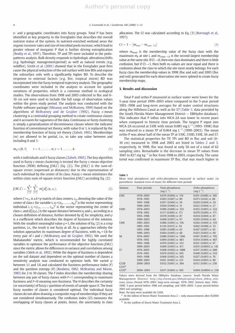
Total P and ortho-P measured in surface water were lower for the5-year time period 1999–2003 when compared to the 5-year period1993–1998 and long-term averages for all water control structuresalong the Hillsboro Canal as well as for S7 (Table 1; data provided bythe South Florida Water Management District — DBHydro database).This indicates that P influx into WCA-2A was lower in recent yearswhen compared to historic time periods. The largest P input intoWCA-2A occurred at S10E with mean 0.085 mg L−1 (1993–1998) thatwas reduced to a mean TP of 0.064 mg L−1 (1999–2003). The meanortho-P was about half of the mean TP at S10C, S10D, S10E, S6 and S7.

The statistical properties for TP, TPi and BD in floc and soil (0–10 cm) measured in 1998 and 2003 are listed in Tables 2 and 3,respectively. In 1998, floc was found at only 56 out of a total of 62sampling sites. Remarkable is the decrease in mean TP values from1047 to 827 mg kg−1 in floc from 1998 to 2003, respectively. The sametrend was confirmed in maximum TP floc, that was much higher in

Table 1Mean total phosphorus and ortho-phosphorus measured in surface water (inparenthesis: standard error of mean) for different time periods

Stations Time periods Total phosphorus Ortho-phosphorus(mg L−1) (mg L−1)

S10C 1978–2003 0.074 (0.004) n: 174 0.051 (0.008) n: 1691978–1992 0.093 (0.007) n: 89 0.073 (0.016) n: 881993–1998 0.057 (0.004) n: 54 0.029 (0.004) n: 541999–2003 0.050 (0.006) n: 31 0.022 (0.004) n: 27

S10D 1978–2003 0.096 (0.006) n: 325 0.052 (0.005) n: 3221978–1992 0.117 (0.009) n: 171 0.070 (0.009) n: 1711993–1998 0.078 (0.006) n: 87 0.034 (0.004) n: 871999–2003 0.068 (0.007) n: 67 0.029 (0.004) n: 64

S10E 1985–2003 0.086 (0.005) n: 156 0.042 (0.004) n: 1551985–1992 0.126 (0.015) n: 34 0.062 (0.008) n: 331993–1998 0.085 (0.008) n: 62 0.047 (0.007) n: 621999–2003 0.064 (0.005) n: 60 0.025 (0.003) n: 60

S6 1974–2003 0.080 (0.063) n: 1306 0.047 (0.003) n: 7051974–1992 0.094 (0.065) n: 483 0.054 (0.004) n: 4671993–1998 0.076 (0.003) n: 352 0.031 (0.003) n: 971999–2003 0.069 (0.003) n: 471 0.035 (0.0003) n: 141

S7 1974–2003 0.068 (0.002) n: 1088 0.037 (0.002) n: 6881974–1992 0.074 (0.003) n: 565 0.040 (0.003) n: 5321993–1998 0.068 (0.002) n: 302 0.027 (0.003) n: 761999–2003 0.051 (0.002) n: 221 0.024 (0.003) n: 80

G328 2000–2003 0.032 (0.001) n: 384 0.012 (0.001) n: 238G337a – – –

G335b 2000–2003 0.017 (0.004) n: 505 0.004 (0.0004) n: 238

Values were derived from the DBHydro Database (source: South Florida WaterManagement District) http://my.sfwmd.gov/dbhydroplsql/show_dbkey_info.main_menu (Period 1978–2003: long-term average; 1978–1992: historic data; 1992–1998: 5-year period before 1998 soil sampling; and 1999–2003: 5-year period before2003 soil sampling).Note: No data were available for S10A.

a At the inflow of Storm Water Treatment Area 2 — only measurements after 9/2004available.

b At the outflow of Storm Water Treatment Area 2.



1998 (4335 mg kg−1) when compared to 2003 (1865 mg kg−1). Themedian, which provides a more robust measure for highly skeweddata such as the TP datasets, showed similar values in floc with730 mg kg−1 (1998) and 751 mg kg−1 (2003); and 485 mg kg−1 (1998)and 433 mg kg−1 (2003) in soil. Total inorganic P accounted for about35% of TP in floc and about 24% in soil in both years. Standarddeviations of soil TP were high with values of 402mg kg−1 in 1998 and316 mg kg−1 in 2003 suggesting large variability across WCA-2A. Bulkdensity values were one order magnitude lower in floc whencompared to soil in both years, which are consistent with findings inother studies (Bruland et al., 2006; Rivero et al., 2007b).

Variations in BD in this system are caused by oxidation of organicmatter due to hydrologic alterations (dry/wet periods) (Reddy et al.,1998) and occasional fires that extend over patches of WCA-2A thatmay burn some of the peat exposing subsurface soil with higher BD(Smith et al., 2001). Assuming a peat accumulation rate of 2.5 mmyr−1

suggested by Craft and Richardson (1993), approximately 12.5 mm ofpeat would have been accumulated within the 5 year sampling period(1998–2003). This translated intomarginal changes inmean BD valuesthat increased by 0.027 g cm−3 andmedians BD by 0.03 g cm−3 (1998–2003). Bruland et al. (2007) observed slight decreases in mean BD (0–10 cm soil) within a 11 year period of 0.03 g cm−3 in WCA-3A Northand South caused mainly by hydrologic alterations.

Maps of TP for floc and soil showed highest values in proximity tothe inflow structures S10 in the north-western part of WCA-2A (Figs. 3and 4). These results are consistent with findings by DeBusk et al.(2001), Grunwald et al. (2004), Corstanje et al. (2006), Bruland et al.(2007) and Rivero et al. (2007b) conducted in various Evergladeswetlands that attributed elevated TP in floc and soils to focal influxpoints. Outflux of P-enriched water from WCA-2A into adjacent,downstream WCA-3 has been observed for the period 1992–2003 byBruland et al. (2007) and more recently by Grunwald et al. (in press).Floc TP values that exceeded 500 mg kg−1 covered 86% and soil TPvalues about 41% of WCA-2A in 1998. In 2003, TP enrichment was alsomost pronounced in proximity to the S10 control structures but withlower values. About 33% of the area showed TP values of larger than500mg kg−1 in soil (2003) and 75% of the area in floc (2003) indicatingan overall decrease in P over the last 5 years. DeBusk et al. (2001) alsofound P-enriched topsoils adjacent to the S10 structures extendinginto the interior of WCA-2A that were moving into the south directionbetween 1990 and 1998.

The ME in our study showed a small under-prediction in floc TP(1998) with ME of −0.132 and larger ones in soil TP (1998) with ME of−0.824 (Table 4). However, the RMSE was much smaller with 247.5 insoil (1998) when compared to 561.0 in floc (1998) indicating highuncertainty in predictions for the latter one that were likely caused bythe low number of observations (n: 56). In 2003, MEs were relativelysmall with slight over-predictions in floc (n: 111) with 0.461 and 0.467in soil (n: 111) (Table 4). The RMSEs in 2003 for floc and soil ranged

from 206.3 (floc; n: 111) up to 285.4 (soil; n: 62) showing similarprediction performance in floc and soil. Important to note is that theerrors in 2003 did only slightly differ for the complete (n: 111) andadjusted (n: 62) datasets indicating that a reduction in observationpoints still provided reliable TP predictions. This is important for thetemporal trajectory analyses, which was conducted using both thecomplete and adjusted 2003 datasets.

Table 3Statistical properties for measured total phosphorus (TP) and total inorganicphosphorus (TPi) in floc and soil (0–10 cm) in WCA-2A in 2003 (n: 111)

Floc Soil (0–10 cm)

TP TPi BD TP TPi BD(mg kg−1) (mg kg−1) (g cm−3) (mg kg−1) (mg kg−1) (g cm−3)

N 111 111 111 111 111 111Mean 827.2 248.7 0.046 550.7 136.5 0.110SE of mean 36.2 13.2 0.003 30.0 13.9 0.003Median 751.3 215.6 0.040 432.8 91.0 0.110Std.dev 381.4 139.2 0.031 316.2 146.6 0.033Skewness 0.59 2.3 5.0 1.34 4.8 3.0Range 1671.2 916.9 0.295 1546.2 1252.9 0.270Min. 194.1 81.7 0.005 155.3 24.2 0.061Max. 1865.3 998.6 0.300 1701.5 1277.1 0.331

Fig. 3. Total phosphorus (TP) in mg kg−1 in floc and soil (0–10 cm) in 1998.

Table 2Statistical properties for measured total phosphorus (TP) and total inorganicphosphorus (TPi) in floc and topsoil (0–10 cm) in WCA-2A in 1998

Floc Soil (0–10 cm)

TP TPi BD TP TPi BD(mg kg−1) (mg kg−1) (g cm−3) (mg kg−1) (mg kg−1) (g cm−3)

N 56 51 51 62 56 51Mean 1047.1 360.8 0.029 692.7 167.8 0.083SE of mean 92.2 58.9 0.002 51.1 23.8 0.004Median 730.4 266.2 0.026 484.6 104.8 0.080Std.dev 690.3 420.4 0.134 402.1 178.1 0.029Skewness 2.4 5.4 2.1 1.8 4.0 0.805Range 4067.7 2923.5 0.080 2015.2 1.167.2 0.140Min. 287.7 95.6 0.010 343.5 44.8 0.030Max. 4355.4 3019.1 0.090 2358.7 1212.0 0.170



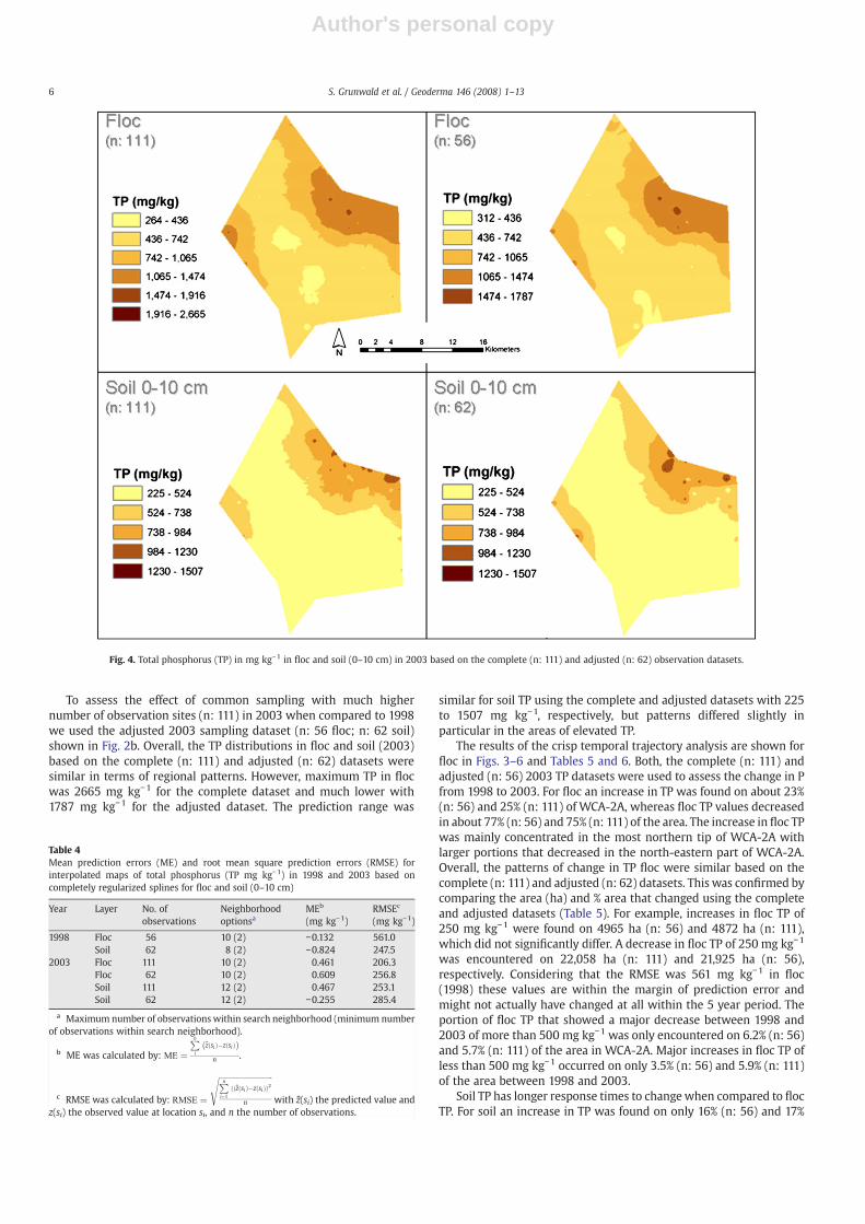
To assess the effect of common sampling with much highernumber of observation sites (n: 111) in 2003 when compared to 1998we used the adjusted 2003 sampling dataset (n: 56 floc; n: 62 soil)shown in Fig. 2b. Overall, the TP distributions in floc and soil (2003)based on the complete (n: 111) and adjusted (n: 62) datasets weresimilar in terms of regional patterns. However, maximum TP in flocwas 2665 mg kg−1 for the complete dataset and much lower with1787 mg kg−1 for the adjusted dataset. The prediction range was

similar for soil TP using the complete and adjusted datasets with 225to 1507 mg kg−1, respectively, but patterns differed slightly inparticular in the areas of elevated TP.

The results of the crisp temporal trajectory analysis are shown forfloc in Figs. 3–6 and Tables 5 and 6. Both, the complete (n: 111) andadjusted (n: 56) 2003 TP datasets were used to assess the change in Pfrom 1998 to 2003. For floc an increase in TP was found on about 23%(n: 56) and 25% (n: 111) of WCA-2A, whereas floc TP values decreasedin about 77% (n: 56) and 75% (n: 111) of the area. The increase in floc TPwas mainly concentrated in the most northern tip of WCA-2A withlarger portions that decreased in the north-eastern part of WCA-2A.Overall, the patterns of change in TP floc were similar based on thecomplete (n: 111) and adjusted (n: 62) datasets. This was confirmed bycomparing the area (ha) and % area that changed using the completeand adjusted datasets (Table 5). For example, increases in floc TP of250 mg kg−1 were found on 4965 ha (n: 56) and 4872 ha (n: 111),which did not significantly differ. A decrease in floc TP of 250 mg kg−1

was encountered on 22,058 ha (n: 111) and 21,925 ha (n: 56),respectively. Considering that the RMSE was 561 mg kg−1 in floc(1998) these values are within the margin of prediction error andmight not actually have changed at all within the 5 year period. Theportion of floc TP that showed a major decrease between 1998 and2003 of more than 500 mg kg−1 was only encountered on 6.2% (n: 56)and 5.7% (n: 111) of the area in WCA-2A. Major increases in floc TP ofless than 500 mg kg−1 occurred on only 3.5% (n: 56) and 5.9% (n: 111)of the area between 1998 and 2003.

Soil TP has longer response times to changewhen compared to flocTP. For soil an increase in TP was found on only 16% (n: 56) and 17%

Fig. 4. Total phosphorus (TP) in mg kg−1 in floc and soil (0–10 cm) in 2003 based on the complete (n: 111) and adjusted (n: 62) observation datasets.

Table 4Mean prediction errors (ME) and root mean square prediction errors (RMSE) forinterpolated maps of total phosphorus (TP mg kg−1) in 1998 and 2003 based oncompletely regularized splines for floc and soil (0–10 cm)

Year Layer No. of Neighborhood MEb RMSEc

observations optionsa (mg kg−1) (mg kg−1)

1998 Floc 56 10 (2) −0.132 561.0Soil 62 8 (2) −0.824 247.5

2003 Floc 111 10 (2) 0.461 206.3Floc 62 10 (2) 0.609 256.8Soil 111 12 (2) 0.467 253.1Soil 62 12 (2) −0.255 285.4

a Maximum number of observations within search neighborhood (minimum numberof observations within search neighborhood).

b ME was calculated by: ME ¼Pni

z sið Þ�z sið Þð Þn .

c RMSE was calculated by: RMSE ¼

ffiffiffiffiffiffiffiffiffiffiffiffiffiffiffiffiffiffiffiffiffiffiffiffiffiffiffiffiPni¼1

ððz sið Þ�z sið ÞÞ2

n

swith z(si) the predicted value and

z(si) the observed value at location si, and n the number of observations.



(n: 111) of WCA-2A, whereas TP values decreased in about 84% (n: 56)and 83% (n: 111) of the area. These results show an inverse spatio-temporal trend with an increase of 393 ha yr−1 of TP that exceeded1000mgkg−1 between1990 and1998 inWCA-2A (DeBusk et al., 2001).The same study reported soil TP concentrations larger than 650 mgkg−1 increased from 10,944 ha (about 25% of the total area) in 1990 to16,344 ha (about 37.8% of the total area) in 1998, an average annualrate of increase of 5%. These findings have to be interpreted withcaution because no prediction errors or variances were reported byDeBusk et al. (2001). Change in soil TP (1998–2003) was notsignificantly different based on the complete (n: 111) and adjusteddatasets (n: 62) (Table 6). Major decrease in soil TP occurred alongthe fringes ofWCA-2Awith 19.4% (0–50 mg kg−1), 20.9% (50–100 mgkg−1), 13.7% (100–150 mg kg−1), 10.0% (150–200 mg kg−1), 13.0%(200–500 mg kg−1) and 5.3% (larger than 500 mg kg−1) of the areabased on change calculations of the complete dataset (n: 111).Considering the RMSE in the range of 247.5mg kg−1 (1998; n: 62) and285.4 mg kg−1 (2003; n: 62) most change in soil TP is within themargin of error. Therefore, it is uncertain based on this crispgeospatial trajectory analysis if TP actually changed in WCA-2A soilswithin the 5 year period. Yet, even a conservative interpretationpoints toward acknowledging increases in soil TP within the interiorof WCA-2A and decreases along the fringes. However, only within asmall portion did this change in TP seem to be beyond the error ofmargin of the geospatial crisp analysis.

The establishment of best management practices in the agriculturalupslope drainage areas has resulted in a significant decline in P influx via

surface waters into WCA-2A at S10C, S10D and S10E between 1998 and2003 (Table 1). This translated intomuch smaller observed and predictedfloc and soil TP in 2003, which suggests that the wetland systemresponded relatively fast within this 5 year period to changes in P influxrecovering towards a more natural/historic P status. DeBusk et al. (2001)suggested a cutoff-value that shifts this wetland from a P-limited intoimpacted state at 500 mg kg−1, whereasWu et al. (1997) indicated that aTP concentration larger than 650 mg kg−1 would elicit cattail invasion inWCA-2A. Bruland et al. (2007) reported increased mean soil TP of 60 mgkg−1 in WCA-3A North, fairly constant soil TP in WCA-3A South, andincreased soil TP of 15mg kg−1 inWCA-3Bwithin a 11 year period (1992–2003). These changes in soil TP were attributed to P influx but are muchsmaller than reported in our study. This can be explained by the muchsmaller mean soil TP values with 461 mg kg−1 (±194 SD) in WCA-3ANorth, 458mg kg−1 (±173 SD) inWCA-3A South, and 385mg kg−1 (±184SD) in WCA-3B (Bruland et al., 2007). The TP concentrations that wepredicted for 2003 were much higher indicating thatWCA-2A is still in aeutrophic state.

Interesting to note is that inWCA-2A both floc and soil TP respondedequally strong to changes in P influx. Floc TP declinewas highest withinthe 5-year period with a maximum of 2900 mg kg−1 south of the S10structures (Fig. 5). Similarly, a patch that showed a rapid decline in soilTP of up to 1439 mg kg−1 was found in the same area (Fig. 6— compare“P-source area”). This suggests that soil P was moved from this sourcearea either into the subsurface soil, incorporated into periphyton ormacrophytes and/or resuspendedand transportedby sheetflow into themarsh interior following hydrologic flow patterns in this wetland. This

Fig. 5. Change in total phosphorus (TP) in floc based on the complete dataset (n: 111) and adjusted dataset (n: 56).



TP source area in soils was matched by a “P-sink” area located south-westwards that showed an increase in soil TP between 1998 and 2003(Fig. 6— compare “P-sink area”). The source to sink ratio for soil TP wasabout4:1 suggesting that besides downstreamredistributionof TPotherprocesses were operating including mineralization and downstreamassimilation. This was confirmed by TPi values (2003) that weresignificantly larger in the “P-sink” area when compared to the marshinterior (data not shown here) suggesting that organic P was convertedinto inorganic P due to increasedmicrobial activity stimulated by higherP content in soils. This “P-sink” area is at risk to shift vegetation patternsfrom sawgrass to cattail that is more adapt to P-enriched soils.

The floc TP changemap indicates that new extensive hotspots haveemerged in the northern most tip of WCA-2A with TP increases of upto 990 mg kg−1. In the same area, the soil TP change map shows muchmore variability of P increases and decreases side-by-side indicatingthat the wetland soils are possibly in transition to a higher P status.Filtering effects of STA 2 along the north-western fringe of WCA-2Ahave been insignificant in floc and soil TP within the consideredsampling period that are within the prediction error margins.

To assess the ecological response of changes in floc and soil TP inWCA-2Awe related TP change trajectories to vegetation patterns. The

Fig. 6. Change in total phosphorus (TP) in soil (0–10 cm) based on the complete dataset (n: 111) and adjusted dataset (n: 62).

Table 5Comparison between TP change maps (1998–2003) for floc using the complete dataset2003 (n: 111) and the adjusted dataset (n: 62)

Lowerbound TP

Upperbound TP

Floc TP datasets — 1998(n: 56) and 2003 (n: 56)

Floc TP datasets — 1998(n: 56) and 2003 (n: 111)

(mg kg−1) (mg kg−1)Area inha

Percentage oftotal area

Area inha


−990 −500 1445 3.52 2449 5.97−500 −250 3124 7.61 2843 6.93−250 0 4965 12.09 4872 11.870 250 22,058 53.74 21,925 53.42250 500 6898 16.81 6610 16.11500 750 1614 3.93 1417 3.45750 2000 881 2.14 867 2.112000 2900 57 0.14 58 0.14Σ 41,042 100 41,041 100

Table 6Comparison between TP change maps (1998–2003) for soil 0–10 cm depth using thecomplete dataset 2003 (n: 111) and the adjusted dataset (n: 62)

Lowerbound TP

Upperbound TP

Soil TP datasets — 1998(n: 62) and 2003 (n: 62)

Soil TP datasets — 1998(n: 62) and 2003 (n: 111)

(mg kg−1) (mg kg−1)Area inha


Area inha


−370 −100 562 1.75 667 1.63−100 −50 1746 4.52 2371 5.78−50 0 3795 9.32 4088 9.960 50 8166 19.55 7955 19.3850 100 7919 18.98 8617 20.99100 150 6754 16.25 5654 13.78150 200 4223 10.32 4126 10.05200 500 5502 13.32 5372 13.09500 1327 2380 6.00 2192 5.34Σ 41,047 100 41,042 100



percent coverage of vegetation in different TP floc and soil changeclasses is shown in Fig. 7a and b. A remarkable increase in cattail wasfound in the TP floc change classes that increased between 1998 and2003. For example, in the TP floc change class −990 to −500 mg kg−1

the cattail coverage increased by 11% and in the TP floc class −500 to−250 mg kg−1 cattail expanded by 12%. In contrast, areas in WCA-2Athat showed a decrease in TP floc between 1998 and 2003 showed aninverse response in vegetation coverage. For example, in the TP flocchange classes 500–750 mg kg−1 cattail coverage decreased by 21.1%,750–2000 mg kg−1 by 24.2%, and 2000–2900 mg kg−1 by 30.1%. As thecoverage in cattail expanded within TP floc change classes thecoverage in sawgrass and freshwater marsh vegetation decreased.Likewise inverse patterns were found for cattail reduction within TPfloc change classes that were associated with expansion in sawgrassand freshwater marsh vegetation. These findings suggest that thestructure of the wetland is undergoing shifts caused by changes in flocP status. Although not as strong as in floc TP, similar trendswere foundfor changes in soil TP shifting vegetation patterns (Fig. 7b). Typically,the magnitude in soil TP change is not as large and it occurs at a muchslower rate when compared to floc. In those areas where soil TPdecreased between 1998 and 2003 the coverage of cattail declined. Forexample, a decrease in 150 to 200 mg kg−1, 200 to 500 mg kg−1 and500 to 1439 mg kg−1 soil TP change (1998–2003) lead to a decline incattail of 3.9%, 8.2%, and 11.5%, respectively. Interestingly, an increasein soil TP (1998–2003) of −50 to −100 mg kg−1 and −100 to −370 mgkg−1 were also associated with a drop in cattail vegetation with 11.5%and 1.1%, respectively. This might be also explained by the rapid dropof mixed hardwood/shrub vegetation from 10.0% and 7.8% and

increase in sawgrass and freshwater marsh vegetation of 21% and8.9%, respectively, in the same two soil TP change classes.

Total P change in floc and soils was heterogeneous withinWCA-2A(Figs. 5 and 6) which was different when compared to the consistentpatches of cattail stands extending mainly south of S10 structures intothe marsh interior. Typically, cattail occurs in monotypic stands thatspreads directionally as a front. This has been also observed inWCA-2A(1995 — South Florida Water Management District; and 2003 — Styset al., 2004 — Florida Fish and Wildlife Conservation Commission)where dense cattail stands were mapped south-southwest of the S10water control structures into the marsh interior fading out intotransitional zones of sawgrass/freshwater marsh vegetation includingmaidencane (Panicum hemitomon), purple bladderwort (Utriculariapurpurea), and spikerush (Eleocharis cellulosa). Clusters of cattailstands also occurred along the North New River Canal in WCA-2A in1995 and 2003. These dense cattail stands lack diversity and areinvasive expanding further in the wetland; thus, from an ecologicalpoint of few are considered not desirable. Cattail spreads extensivelyby rhizomes so that half a hectare of cattail may consist of only a fewindividual plants. Since cattail is tolerant of continuous inundationand seasonal drawdowns, the rhizomes are under water and wellprotected against fire if inundated and rapidly colonize wetlands. Thespatial association between higher levels of soil TP and cattail hasbeen documented in varied hydrologic units within the Everglades byWu et al. (1997), Newman et al. (1998), and Noe et al. (2001). Ourstudy enabled to relate temporal trajectories in floc/soil TP to changesin vegetation patterns to assess if those relationships persist throughspace and time. Such space–time investigations are relatively rare due

Fig. 7. Percent coverage of different vegetation classes in total phosphorus (TP) floc (a) and soil (b) change classes between 1998 and 2003. (Data sources: South Florida WaterManagement District — 1995 land use/cover map; Stys et al., 2004 — Florida Fish and Wildlife Conservation Commission — 2003 vegetation and habitat map Florida).



to the costs and labor associated with floc/soil monitoring. Anotherunique aspect of our study is the spatio-temporal characterization ofboth floc and soil TP. Although the relationships between TP flocchange (1998–2003) and vegetation were stronger than between TPsoil change (1998–2003) and vegetation it must be noted that theuncertainty to map TP floc change was larger than for TP soil change(compare Table 4).

The implications for understanding the space–time relationshipsbetween floc TP, soil TP and vegetation are enormous. Vegetationpatterns can be mapped rapidly using satellite technology and aerialphotographs (Grunwald and Lamsal, 2006; Rivero et al., 2007a)providing dense exhaustive land cover datasets for wetlands such asWCA-2A or other aquatic ecosystems. Grunwald (2006) describedseveral hybrid geospatial models that combine dense exhaustivegeospatial data (e.g. vegetation data) to predict sparsely measured soilproperties (e.g. soil TP) using cokriging, regression kriging or similarmultivariate geostatistical methods. A demonstration to predict soil TPcontinuously across a wetland using satellite-derived vegetationpatterns and regression kriging was given by Grunwald et al. (2007).Such integrative analyses that focus on multiple ecosystem compo-nents (e.g. soil nutrient status, vegetation patterns, periphytoncommunities) are well suited to improve our understanding ofecosystem behavior in space and time. Ogden et al. (2005) presenteda conceptual ecological modeling framework for the Evergladesintegrating several ecological stressors outlining the need to betterexplain all ecosystem components including soil nutrient status. Thereare tremendous needs to populate and validate ecological simulationmodels with spatially and temporally explicit floc/soil TP and otherbiogeochemical properties. Therefore, our study closed an importantresearch gap. Numerous mechanistic simulation models for wetlandsand aquatic systems have been developed that lack spatially-explicitsoil data. For example, Diffendorfer et al. (2001) presented thespatially heterogeneous ecosystem model covering different fresh-water habitat types in the Everglades to model changing patterns ofbiomass, energy flux, and species composition by. Other mechanisticmodels that simulate ecosystem processes are the Ecological DynamicSimulation Model (EDYS) by Childress et al. (2002) and the mechan-istic Everglades Landscape Model by Fitz et al. (2004).

The crisp geospatial analysis revealed the uncertainties to map TPchange in absolute values. Thus, an alternative method of fuzzy c-mean clustering was performed to identify the change in pedo-patterns rather than the change in absolute values of TP. We used afuzziness exponent of 1.4 and minimized the F (0.290) and H (0.266)coefficients with a set of 8 fuzzy classes (Table 7). The class centroidsderived from the fuzzy c-mean classification are documented inTable 8, interpolation errors in Table 9, and interpolated membershipmaps for each of the 8 classes for 1998 are shown in Fig. 8 and for 2003in Fig. 9. Mean errors and RMSEs were slightly higher in 1998 whencompared to 2003. Interesting to note is the differences in the spatialdistribution of membership values that represent pedo-patternsderived from TP, TPi, BD, and geographic coordinates. Class 1 wasmore pronounced in the western fringe in 1998 and more or less

homogenous across WCA-2A in 2003. This class was characterized bymedium BD, high TP with a class centroid of 1337 mg kg−1, andmoderate high TPi with class centroid 390 mg kg−1 and lowestlongitude centroid out of all classes with −80.5088°. Classes 2 and 4were relatively insensitive to change in membership values between1998 and 2003 representing moderate high TP and TPi values. Butboth were mapped out with high membership values in the northernedge (class 2) and along the southwestern edge (class 4), respectively,as indicated by the latitude and longitude centroids. Class 3memberships showed one hotspot on the 1998 map located south ofinflow structures and represented the largest TP and TPi centroidsfound in WCA-2A. This hotspot disappeared from the 2003 map. Thedifferences in membership values were pronounced in class 5 in 1998and 2003, with decreasing values in 2003. Class 5 showed low BDwithclass centroids of 0.033 g cm−3, moderate high TP with a centroid of557 mg kg−1 and relatively low TPi with 195 mg kg−1. The geographiclocation of class 5 was found close to the drainage outlet ofWCA-2A asindicated by the lowest latitude centroid of 26.2765° found in thedataset. Memberships in class 6were highest in the north-eastern partof WCA-2A confirming the high impact of TP in floc and soil in thislocation. The TP centroid was high with 1264 mg kg−1 in class 6 butshowed a relatively low TPi centroid value of only 284 mg kg−1

suggesting that more P was present in form of organic P forms. Theappearance of high membership values (class 6) was speckled in 1998and 2003 in the north-eastern portion indicating that the likelihood ofencountering characteristics pedo-patterns of class 6 ranged from

Table 7Fuzziness performance index (F) and modified partition entropy (H) for different sets offuzzy classes (fuzziness exponent φ=1.4)

Number of classes F H

2 0.540 0.6123 0.407 0.4474 0.358 0.3795 0.309 0.3466 0.307 0.3047 0.307 0.2948 0.290 0.2669 0.319 0.28010 0.320 0.282

Table 8Class centroids derived from fuzzy c-mean classification using the entire dataset (i.e.,1998 and 2003 floc and soil data)

Classes Variables

BD TP TPi Latitude Longitude(g cm−3) (mg kg−1) (mg kg−1) (deg.) (deg.)

1 0.062 1336.7 389.6 26.3156 −80.50882 0.111 548.3 129.0 26.4107 −80.43983 0.068 2382.2 1513.4 26.3672 −80.38874 0.112 413.1 98.9 26.2876 −80.45825 0.033 557.1 194.6 26.2765 −80.39216 0.050 1263.5 283.9 26.3446 −80.33797 0.047 796.9 258.7 26.3886 −80.43398 0.094 478.4 108.4 26.2838 −80.3369

Table 9Mean prediction errors (ME) and root mean square prediction errors (RMSE) forinterpolated maps of membership values [range: 0–1] for 8 fuzzy classes in 1998 (n: 62)and 2003 (n: 111)

Year Class Neighborhood optionsa ME RMSE

1998 1 8 (2) −0.0048 0.1372 10 (2) −0.0025 0.1283 10 (2) 0.0024 0.1364 10 (2) 0.0019 0.0955 10 (2) 0.0035 0.1186 12 (2) −0.0028 0.2017 12 (2) 0.0026 0.1828 10 (2) 0.0014 0.062CI 12 (2) 0.0013 0.202

2003 1 12 (2) −0.0032 0.1062 10 (2) −0.0019 0.0823 15 (2) 0.0004 0.0564 12 (2) 0.0012 0.0855 12 (2) 0.0003 0.0826 12 (2) 0.0006 0.1457 12 (2) 0.0012 0.0758 12 (2) −0.0006 0.085CI 10 (2) −0.0013 0.198

a Maximum numbers within search neighborhood (minimum number within searchneighborhood).



very high to low. Class 7 memberships were highest in the northernsection of WCA-2A with the lowest BD centroid of 0.047 g cm−3

encountered within WCA-2A and elevated TP as indicated by acentroid of 797 mg kg−1. This class has diminished in impact in 2003

with much lower membership values when compared to the 1998map. Pedo-patterns of class 7 are much more muted in 2003indicating that homogenization has taken place. The lowest TP classcentroids weremapped into class 8with 478mg kg−1 and very low TPi

Fig. 8. Membership values of fuzzy classes in 1998 derived from fuzzy c-mean classification.

Fig. 9. Membership values of fuzzy classes in 2003 derived from fuzzy c-mean classification.



with 108 mg kg−1. This is likely to present the least nutrient-impactedareas in WCA-2A.

The CI maps showed contrasting patterns for 1998 and 2003(Fig. 10). This index measures the uncertainty of class allocation. If theclass membership values for two or more continuous classes varycontinuously over geographic space there will be locations wheremiNmj and locations where mjNmi. A location where mi is replaced bymj as the dominant value marks a transition both in attribute andgeographic space from class i to j, i.e., it is a local boundary. Becausethe mi and mj values vary continuously over geographic space, theremay be regions where their values are very similar, in which case itwill not be clear which class dominates, and this results in confusion,expressed by the CI. The CI was highest, i.e., showed large confusion, inthe interior and few spots along the edges of WCA-2A in 1998.Speckled patterns of moderate to high CI were encountered in 2003that extended in a U-shape across WCA-2A. In particular, the areasthat showed nutrient enrichment seemed to coincide with highconfusion about the class to which the site most likely belongs. Thelowest CI values in 2003 were found in the northern section of WCA-2A indicating that one class (highest memberships in class 2)dominated with less confusion about class assignments. This wasalso true for the southern section of WCA-2A where highestmemberships were found in class 5.

The fuzzy-based analysis was able to integrate multiple key soilproperties that responded to nutrient influx, mineralization, hydro-logic fluctuations, fire etc. into a spatio-temporal framework. There-fore, synergistic effects were mapped in form of pedo-patterns thatdocumented how the wetland system responded to biogeochemicalprocesses and external drivers. The fuzzy classes represented differentresponse ratios among variables, i.e. different ratios between TP:TPi:BD:latitude:longitude. Since the membership values are standardized(0 to 1) they are intuitive to grasp and facilitate to compare patternsacross space and at different time periods. Thus, the fuzzy setapproach complemented the uni-dimensional crisp temporal trajec-tory analysis that was constrained to characterize only TP patterns.Even more biogeochemical properties could be incorporated intofuzzy sets in future analysis to account for additional processes and

stresses. However, costs and labor to measure additional biogeo-chemical properties may be the limiting factor. Membership valuesmap the degrees of belonging. Zhu (2005) pointed out that fuzzy logicis about possibility, whereas crisp logic is about probability. Possibilitymay be more appropriate for temporal trajectory analysis becausesynergistic responses are mapped in continuously evolving wetlandsystems shifting pedo-patterns in space and time. Since fuzzy-basedmembership values are surrogates they are not intended to replacecrisp temporal trajectory analysis but serve as complimentary input todocument shifts in wetlands.

4. Summary and conclusions

We presented a temporal trajectory approach based on fuzzy setsthat accounted for biogeochemical processes and external drivers thatimpacted WCA-2A between 1998 and 2003. Pedo-patterns weresurrogates of TP, TPi, BD and geographic coordinates. Total P was usedas a key indicator that describes the nutrient status of a subtropicalwetland. Total inorganic P served as an indicator for organic turnoverand nutrient induced microbial activity; and BD responded tohydrologic alterations/shifts and natural events such as fire. Theholistic space–time modeling focused on pedo-patterns that providedsignatures linking ecosystem processes to properties. These spatio-temporal pedo-patterns may serve as future metrics to monitor therecovery of this wetland ecosystem to a more natural state.

The uni-dimensional temporal trajectory analysis was focused onlyon TP in floc and soils. Spatial relationships between P change (1998–2003) in floc and soils and vegetation were found in this wetlandindicating that cattail expansion was associated with P enrichment. Itwas shown that the differences in spatial sampling designs (1998 and2003) did not have a major impact on the crisp temporal trajectoryanalysis. This provided confidence in our approach although TP mapsshould be interpreted with caution since prediction errors, inparticular for TP floc, were relatively high. Although P has beenidentified as a key property in this type of ecosystem a uni-dimensional approach is limiting. In conclusion, criteria for monitor-ing of ecosystem patterns in space and time ideally should (i) use a

Fig. 10. Confusion index derived from fuzzy c-mean classification for 1998 and 2003.



metric on a continuous standardized scale rather a crisp scale,(ii) adopt a multi-dimensional approach integrating multiple proper-ties that respond to internal biogeochemical processes and externaldrivers, (iii) use standard ecosystem properties that are easy tomeasure allowing repetition of monitoring in space and time,(iv) include above and below-ground ecosystem properties tocharacterize responses that occur at different spatial and temporalscales, and (iv) be transferable to other similar ecosystems. Moreresearch that explicitly incorporates differential behavior of ecosys-tem properties in space and time is needed to improve our under-standing of shifts in ecosystems.

Acknowledgements

We would like to thank C. Fitz, N. Wang, and J. Godin of the SouthFloridaWaterManagement District for assisting in the development ofthe stratified-random sampling design used in the 2003 sampling, T.Jones of Aircoastal Helicopters Inc. for his support of mapping in 2003,W. DeBusk for sampling in 1998, and S. Newman for her support ofsampling in 2003, and Y. Wang of the Wetland BiogeochemistryLaboratory for her work with the laboratory analyses.

References

Amini, M., Afyuni, M., Fathianpour, N., Khademi, K., Flühler, H., 2005. Continuous soilpollution mapping using fuzzy logic and spatial interpolation. Geoderma 124,223–233.

Anderson, J.M., 1976. An ignition method for determination of total phosphorus in lakesediments. Water Res. 10, 329–331.

Bezdek, J.C., Pal, S.K., 1992. Fuzzy Models for Pattern Recognition: Methods that Searchfor Structures in Data. Institute of Electrical and Electronics Engineers, New York.

Braganto, G., 2004. Fuzzy continuous classification and spatial interpolation inconventional soil survey for soil mapping of the lower Piave plain. Geoderma 118,1–16.

Brown, D.G., Duh, J.-D., 2003. Spatial simulation for translating from land use to landcover. Int. J. Geogr. Inf. Sci. 17, 1–26.

Bruland, G.L., Grunwald, S., Osborne, T.Z., Reddy, K.R., Newman, S., 2006. Spatialdistribution of soil properties in Water Conservation Area 3 of the Everglades. SoilSci. Soc. Am. J. 70, 1662–1676.

Bruland, G.L., Osborne, T.Z., Reddy, K.R., Grunwald, S., Newman, S., DeBusk, W.F., 2007.Recent changes in soil total phosphorus in the Everglades: Water ConservationArea 3. J. Environ. Monit. Assess. 129, 379–395.

Burrough, P.A., van Gaans, P.F.M., Hootsmans, R., 1997. Continuous classification in soilsurvey: spatial correlation, confusion and boundaries. Geoderma 77, 115–135.

Childress, W.M., Coldren, C.L., McLendon, T., 2002. Applying a complex, generalecosystemmodel (EDYS) in large-scale landmanagement. Ecol. Model. 153, 97–108.

Corstanje, R., Grunwald, S., Reddy, K.R., Osborne, T.Z., Newman, S., 2006. Assessment ofthe spatial distribution of soil properties in a northern Everglades. J. Environ. Qual.35, 938–949.

Craft, C.B., Richardson, C.J., 1993. Peat accreation and N, P and organic C accumulation innutrient-enriched and unenriched Everglades peatlands. Ecol. Appl. 3, 446–458.

de Bruin, S., Stein, A., 1998. Soil–landscape modelling using fuzzy c-means clustering ofattribute data derived from a digital elevation model (DEM). Geoderma 83, 17–33.

DeBusk, W.F., Newman, S., Reddy, K.R., 2001. Spatio-temporal patterns of soilphosphorus enrichment in Everglades Water Conservation Area 2A. J. Environ.Qual. 30, 1438–1446.

Diffendorfer, J.E., Richards, P.M., Dalrymple, G.H., DeAngelis, D.L., 2001. Applying linearprogramming to estimate fluxes in ecosystems or food webs: an example from theherpetological assemblage of the freshwater Everglades. Ecol. Model. 144, 99–120.

Fitz, C., Sklar, F., Waring, T., Voinov, A., Constanza, R., Maxwell, T., 2004. Developmentand application of the Everglades Landscape Model. In: Constanza, R., Voinov, A.(Eds.), Landscape Simulation Modeling — a Spatially Explicit Dynamic Approach.Springer, New York, pp. 143–172.

Grunwald, S., 2006. What do we really know about the space–time continuum of soil–landscapes. In: Grunwald, S. (Ed.), Environmental Soil–Landscape Modeling —Geographic Information Technologies and Pedometrics. CRC Press, New York, pp. 3–36.

Grunwald, S., Lamsal, S., 2006. Emerging geographic information technologies and soilinformation systems. In: Grunwald, S. (Ed.), Environmental Soil–LandscapeModeling — Geographic Information Technologies and Pedometrics. CRC Press,New York, pp. 127–154.

Grunwald, S., McSweeney, K., Rooney, D.J., Lowery, B., 2001. Soil layer models createdwith profile cone penetrometer data. Geoderma 103, 181–201.

Grunwald, S., Reddy, K.R., Newman, S., DeBusk, W.F., 2004. Spatial variability,distribution and uncertainty assessment of soil phosphorus in a south Floridawetland. Environmetrics 15, 811–825.

Grunwald, S., Rivero, R.G., Reddy, K.R., 2007. Understanding spatial variability and itsapplication to biogeochemistry analysis. In: Sarkar, D., Datta, R., Hannigan, R.

(Eds.), Environmental Biogeochemistry — Concepts and Case Studies. Elsevier,Berlin, pp. 435–462.

Grunwald, S., Reddy, K.R., Osborne, T.Z., Bruland, G.L., in press. Soil and vegetativepatterns and their variability in space across the Greater Everglades. J. Environ.Qual.

Jensen, J.R., Rutchey, K., Koch, M.S., Narumalani, S., 1995. Inland wetland changedetection in the Everglades Water Conservation Area 2A using a time series ofnormalized remotely sensed data. Photogramm. Eng. Remote Sensing 61 (2),199–209.

King, R., Richardson, C., Urban, D., Romanowicz, E., 2004. Spatial dependency ofvegetation-environmental linkages in an anthropogenically influenced wetlandecosystem. Ecosystems 7, 75–97.

Lagacherie, P., Cazemier, D.R., van Gaans, P.F.M., Burrough, P.A., 1997. Fuzzy k-meansclustering of fields in an elementary catchment and extrapolation to a larger area.Geoderma 77, 197–216.

McBratney, A.B., de Grujiter, J.J., 1992. A continuum approach to soil classification bymodified fuzzy k-means with extragrades. Soil Sci. 43, 159–175.

McBratney, A.B., Moore, A.W., 1985. Application of fuzzy sets to climatic classification.Agric. For. Meteorol. 35, 165–185.

McBratney, A.B., Odeh, I.O.A., 1997. Application of fuzzy sets in soil science: fuzzy logic,fuzzy measurements and fuzzy decisions. Geoderma 77, 85–113.

McCormick, P.V., Stevenson, R.J., 1998. Periphyton as a tool for ecological assessmentand management in the Florida Everglades. J. Phycol. 34, 726–733.

McCormick, P.V., Newman, S., Miao, S., Reddy, K.R., Fontaine, T.D., 2002. Effects ofanthropogenic phosphorus inputs in the Everglades. In: Porter, J.W., Porter, K.G.(Eds.), The Everglades, Florida Bay and Coral Reefs of the Florida Keys. CRC Press,New York.

Minasny, B., McBratney, A.B., 1999. Fuzzy k-mean with extragrade program — FuzMEversion 1.0. Australian Centre for Precision Agriculture, McMillan Building A05, TheUniversity of Sydney, NSW 2006. Available at http://www.usyd.edu.au/su/agric/acpa/fkme/FkME.html (verified Aug. 30, 2007).

Newman, S., Schuette, J., Grace, J.B., Rutchey, K., Fontaine, T., Reddy, K.R., Pietrucha, M.,1998. Factors influencing cattail abundance in the northern Everglades. Aquat. Bot.60, 265–280.

Noe, G.B., Childers, D.L., Jones, R.D., 2001. Phosphorus biogeochemistry and the impactof phosphorus enrichment: why is the Everglades so unique? Ecosystems 4,603–624.

Odeh, I.O.A., McBratney, A.B., Chittleborough, D.J., 1992. Soil pattern recognition withfuzzy c-means: Applications to classification and soil–landform interrelationships.Soil Sci. Soc. Am. J. 56, 505–516.

Ogden, J.C., Davis, S.M., Barnes, T.K., Jacobs, K.J., Gentile, J.H., 2005. Total systemconceptual ecological model. Wetlands 25 (4), 955–979.

Pijanowski, B.C., Brown, D.G., Shellito, B.A., Manik, G.A., 2002. Using Neural Networksand GIS to Forecast Land Use Changes: A Land Transformation Model.

Porter, J.W., Porter, K.G. (Eds.), 2002. The Everglades, Florida Bay and Coral Reefs of theFlorida Keys. CRC Press, New York.

Reddy, K.R., White, J.R., Wright, A., Chua, T., 1997. Influence of phosphorus loading onmicrobial processes in the soil and water column of wetlands. In: Reddy, K.R.,O'Connor, G.A., Schelske, G.L. (Eds.), Phosphorus Biogeochemistry in SubtropicalEcosystems. Lewis Publ., New York, pp. 249–273.

Reddy, K.R., Wang, Y., DeBusk, W.F., Fisher, M.M., Newman, S., 1998. Forms of soilphosphorus in selected hydrologic units of the Florida Everglades. Soil Sci. Soc. Am.J. 62, 1134–1147.

Rivero, R.G., Grunwald, S., Bruland, G.L., 2007a. Incorporation of spectral data intomultivariate geostatistical models to map soil phosphorus variability in a Floridawetland. Geoderma 140, 428–443.

Rivero, R.G., Grunwald, S., Osborne, T.Z., Reddy, K.R., Newman, S., 2007b. Characteriza-tion of the spatial distribution of soil properties in Water Conservation Area-2A,Everglades, Florida. Soil Sci. 172 (2), 149–166.

Roubens, M., 1982. Fuzzy clustering algorithms and their cluster validity. Eur. J. Oper.Res. 10, 294–301.

Smith, S., Newman, S., Garrett, P.B., Leeds, J.A., 2001. Differential effects of surface andpeat fire on soil constituents in a degraded wetland of the northern FloridaEverglades. J. Environ. Qual. 30, 1998–2005.

South Florida Water Management District, 1995. Land Cover/Use Map South Florida.Accessible: http://www.fgdl.org (verified: 10/2006).

Stys, B., Kautz, R., Reed, D., Kertis, M., Kawula, R., Keller, C., Davis, A., 2004. Office ofEnvironmental Services, Florida Fish andWildlife Conservation Commission. DigitalFlorida Vegetation and Land Cover Map, Derived from 2003 Landsat ThematicMapper Satellite Images.

U.S. Environmental Protection Agency, 1993. Methods for the Determination ofInorganic Substances in Environmental Samples. Environmental MonitoringSystems Lab, Cincinnati, OH.

Van Meirvenne, M., Pannier, M.J., Hofman, G., Louwagie, G., 1996. Regional character-ization of the long-term change in soil organic carbon under intensive agriculture.Soil Use Manage. 12, 86–94.

Wu, Y., Sklar, F.H., Rutchey, K., 1997. Analysis and simulations of fragmentation patternsin the Everglades. Ecol. Appl. 7 (1), 268–276.

Zaheh, L.A., 1965. Fuzzy sets. Inf. Control 8, 338–353.Zhu, A.-X., 2005. Fuzzy logic models. In: Grunwald, S. (Ed.), Environmental Soil–

Landscape Modeling— Geographic Information Technologies and Pedometrics. CRCPress, New York, NY, pp. 215–239.


author's personal copy - uf/ifas · author's personal copy temporal trajectories of...

Documents