learning and coding in biological neural networks - harvard
TRANSCRIPT

Learning and coding in biological neural networks
A thesis presented
by
Ila Rani Fiete
to
The Department of Physics
in partial fulfillment of the requirements
for the degree of
Doctor of Philosophy
in the subject of
Physics
Harvard University
Cambridge, Massachusetts
December 2003

c�
2003 Ila Rani Fiete
All rights reserved

for my parents
Mummy–Babuji
Abstract
Learning and coding in biological neural networks
Ila Rani Fiete
Thesis Advisor: Professor H. S. Seung
Committee Members: Professors D. S, Fisher (chair), C. M. Marcus and V. N. Murthy
How can large groups of neurons that locally modify their activities learn to col-
lectively perform a desired task? Do studies of learning in small networks tell us anything
about learning in the fantastically large collection of neurons that make up a vertebrate
brain? What factors do neurons optimize by encoding sensory inputs or motor commands
in the way they do? In this thesis I present a collection of four theoretical works: each
of the projects was motivated by specific constraints and complexities of biological neural
networks, as revealed by experimental studies; together, they aim to partially address some
of the central questions of neuroscience posed above.
We first study the role of sparse neural activity, as seen in the coding of sequential
commands in a premotor area responsible for birdsong. We show that the sparse coding of
temporal sequences in the songbird brain can, in a network where the feedforward plastic
weights must translate the sparse sequential code into a time-varying muscle code, facilitate
learning by minimizing synaptic interference.
Next, we propose a biologically plausible synaptic plasticity rule that can perform
goal-directed learning in recurrent networks of voltage-based spiking neurons that interact
through conductances. Learning is based on the correlation of noisy local activity with
a global reward signal; we prove that this rule performs stochastic gradient ascent on the

v
reward. Thus, if the reward signal quantifies network performance on some desired task,
the plasticity rule provably drives goal-directed learning in the network.
To assess the convergence properties of the learning rule, we compare it with
a known example of learning in the brain. Song-learning in finches is a clear example
of a learned behavior, with detailed available neurophysiological data. With our learning
rule, we train an anatomically accurate model birdsong network that drives a sound source
to mimic an actual zebrafinch song. Simulation and theoretical results on the scalability
of this rule show that learning with stochastic gradient ascent may be adequately fast to
explain learning in the bird.
Finally, we address the more general issue of the scalability of stochastic gradient
learning on quadratic cost surfaces in linear systems, as a function of system size and task
characteristics, by deriving analytical expressions for the learning curves.

Contents
Title Page . . . . . . . . . . . . . . . . . . . . . . . . . . . . . . . . . . . . . . iDedication . . . . . . . . . . . . . . . . . . . . . . . . . . . . . . . . . . . . . . iiiAbstract . . . . . . . . . . . . . . . . . . . . . . . . . . . . . . . . . . . . . . . ivTable of Contents . . . . . . . . . . . . . . . . . . . . . . . . . . . . . . . . . . viList of Figures . . . . . . . . . . . . . . . . . . . . . . . . . . . . . . . . . . . . viiiAcknowledgments . . . . . . . . . . . . . . . . . . . . . . . . . . . . . . . . . . ix
1 Introduction 11.1 Local activity-dependent synaptic plasticity . . . . . . . . . . . . . . . . . 5
1.1.1 Hebb’s proposal . . . . . . . . . . . . . . . . . . . . . . . . . . . 51.1.2 Experimental observations of local activity-induced plasticity . . . 51.1.3 Theoretical successes of local activity-based learning rules . . . . . 7
1.2 Reinforcement signals in the brain . . . . . . . . . . . . . . . . . . . . . . 81.2.1 Behavioral paradigm for reward-based learning . . . . . . . . . . . 101.2.2 The physiology of reward and punishment in insects . . . . . . . . 101.2.3 The physiology of reward in mammals . . . . . . . . . . . . . . . . 121.2.4 Experience-dependent reward coding . . . . . . . . . . . . . . . . 13
1.3 Learning complex tasks with simple rewards: insights from psychology . . 141.4 Contributions from the field of machine learning . . . . . . . . . . . . . . . 171.5 Learning many tasks simultaneously: compartmentalization? . . . . . . . . 201.6 Quick overview . . . . . . . . . . . . . . . . . . . . . . . . . . . . . . . . 221.7 Chapter summaries . . . . . . . . . . . . . . . . . . . . . . . . . . . . . . 24
2 Background and perspective 282.1 What is a neuron? . . . . . . . . . . . . . . . . . . . . . . . . . . . . . . . 292.2 Neural networks . . . . . . . . . . . . . . . . . . . . . . . . . . . . . . . . 312.3 Modern topics in theoretical neuroscience . . . . . . . . . . . . . . . . . . 33
3 Temporal sparseness of the premotor drive is important for rapid learning ina model of birdsong 363.1 Abstract . . . . . . . . . . . . . . . . . . . . . . . . . . . . . . . . . . . . 363.2 Introduction . . . . . . . . . . . . . . . . . . . . . . . . . . . . . . . . . . 373.3 Methods . . . . . . . . . . . . . . . . . . . . . . . . . . . . . . . . . . . . 403.4 Results . . . . . . . . . . . . . . . . . . . . . . . . . . . . . . . . . . . . . 433.5 Discussion. . . . . . . . . . . . . . . . . . . . . . . . . . . . . . . . . . . 51
vi

Contents vii
3.6 Appendix . . . . . . . . . . . . . . . . . . . . . . . . . . . . . . . . . . . 56
4 A biologically plausible learning rule for reward optimization in networks ofconductance-based spiking neurons 584.1 Introduction . . . . . . . . . . . . . . . . . . . . . . . . . . . . . . . . . . 594.2 Learning rule . . . . . . . . . . . . . . . . . . . . . . . . . . . . . . . . . 604.3 Arbitrary noise . . . . . . . . . . . . . . . . . . . . . . . . . . . . . . . . 634.4 Gaussian noise . . . . . . . . . . . . . . . . . . . . . . . . . . . . . . . . 664.5 Generalization of the learning rule . . . . . . . . . . . . . . . . . . . . . . 68
4.5.1 Learning with excitatory and inhibitory conductances . . . . . . . . 694.5.2 Noise in currents . . . . . . . . . . . . . . . . . . . . . . . . . . . 71
4.6 Discussion . . . . . . . . . . . . . . . . . . . . . . . . . . . . . . . . . . . 71
5 Rapid learning of birdsong by reinforcement of variation in spiking networks 765.1 Abstract . . . . . . . . . . . . . . . . . . . . . . . . . . . . . . . . . . . . 765.2 Results . . . . . . . . . . . . . . . . . . . . . . . . . . . . . . . . . . . . . 835.3 Methods . . . . . . . . . . . . . . . . . . . . . . . . . . . . . . . . . . . . 92
5.3.1 Premotor network . . . . . . . . . . . . . . . . . . . . . . . . . . . 925.3.2 Sound production . . . . . . . . . . . . . . . . . . . . . . . . . . . 955.3.3 Sound comparison and reward . . . . . . . . . . . . . . . . . . . . 975.3.4 Learning . . . . . . . . . . . . . . . . . . . . . . . . . . . . . . . 995.3.5 Scaling simulations . . . . . . . . . . . . . . . . . . . . . . . . . . 99
5.4 Appendix: calculation of the learning curve in a linear model birdsongnetwork . . . . . . . . . . . . . . . . . . . . . . . . . . . . . . . . . . . . 1005.4.1 The network and learning rule . . . . . . . . . . . . . . . . . . . . 1005.4.2 Learning curves . . . . . . . . . . . . . . . . . . . . . . . . . . . . 1025.4.3 Scaling . . . . . . . . . . . . . . . . . . . . . . . . . . . . . . . . 1035.4.4 Application to birdsong learning . . . . . . . . . . . . . . . . . . . 104
6 Learning by stochastic gradient descent on anisotropic cost surfaces: scalingof learning time with system size and task difficulty 1076.1 Learning curve . . . . . . . . . . . . . . . . . . . . . . . . . . . . . . . . 1126.2 Bounds on the learning rate . . . . . . . . . . . . . . . . . . . . . . . . . . 1146.3 Learning time and scaling . . . . . . . . . . . . . . . . . . . . . . . . . . . 116
6.3.1 Comparison of anisotropic and isotropic stochastic learning . . . . 1206.3.2 Comparison with direct gradient learning . . . . . . . . . . . . . . 122
6.4 Applications to neural network learning . . . . . . . . . . . . . . . . . . . 1246.5 Appendix . . . . . . . . . . . . . . . . . . . . . . . . . . . . . . . . . . . 128
6.5.1 Derivation of ��� and bounds on � . . . . . . . . . . . . . . . . . . . 1286.5.2 Inverse of the � eigenvector matrix . . . . . . . . . . . . . . . . . 1296.5.3 Generalization to � �� output units . . . . . . . . . . . . . . . . 130
Bibliography 132

List of Figures
3.1 A schematic of the model birdsong network. . . . . . . . . . . . . . . . . . 403.2 Sample inputs and outputs of the nonlinear model birdsong learning network. 443.3 Learning curves from a nonlinear model network simulation of birdsong
learning: learning time depends on the number of bursts fired per HVCneuron. . . . . . . . . . . . . . . . . . . . . . . . . . . . . . . . . . . . . 46
3.4 A geometric interpretation of learning on a quadratic error function. . . . . 493.5 Numerical eigenvalue calculation to check the mean-field results. . . . . . . 523.6 Learning speed scales inversely with the number bursts per HVC neuron:
numerical and analytical results with linear analysis. . . . . . . . . . . . . 53
5.1 Illustration of the learning rule in a general framework. . . . . . . . . . . . 795.2 The model song-learning network. . . . . . . . . . . . . . . . . . . . . . . 855.3 Results from the model song-learning network. . . . . . . . . . . . . . . . 865.4 Scaling of learning speed with network size. . . . . . . . . . . . . . . . . . 915.5 Delaying the instantaneous eligibility. . . . . . . . . . . . . . . . . . . . . 95
6.1 Learning time depends not just on system size but on details of the learningproblem. . . . . . . . . . . . . . . . . . . . . . . . . . . . . . . . . . . . . 110
6.2 Eigenvalue spectrum of the recursion matrix � , as computed numericallywith derived bounds on the learning rate. . . . . . . . . . . . . . . . . . . . 119
6.3 Relevance of stochastic gradient analysis to learning in neural networks. . . 1256.4 Eigenvalues of the cost surface in a real-world problem of neural network
digit recognition. . . . . . . . . . . . . . . . . . . . . . . . . . . . . . . . 1266.5 Demonstration of the effective dimensionality of the digit data set. . . . . . 127
viii

Acknowledgments
For giving me the chance to enter into the vast world in neuroscience, and for
being my superb and incisive guide, I am deeply indebted to my advisor Sebastian Seung.
His openness to new directions, uncanny ability to simultaneously and easily grasp both
minute details and panoramic vistas of any issue, and his remarkable clarity of thought and
exposition, are qualities I can only aspire to. I am grateful to him for allowing me much
independence in work and travel, yet also providing me with guidance and advice whenever
I needed it. Above all else, I thank Sebastian for being not just an inspiring and generous
advisor, but a wonderful friend.
I am very lucky to have Daniel Fisher as my Harvard advisor, and am grateful
to him for taking an active interest in my work, and for many helpful and interesting dis-
cussions. He made it possible for me to explore new directions: without his interest and
involvement, I am sure I wouldn’t be able to present this (gasp!) blatantly neuroscience
thesis for a degree in Physics. Daniel has persistently kept me on track, and given me ex-
cellent and timely advice: to be the recipient of his very sincere concern for my scientific
development, I consider myself privileged.
I am fortunate to have had several fantastic collaborators: many thanks go to
Richard Hahnloser, Michale Fee, and Alexay Kozhevnikov for exciting conversations and
for introducing me to the study of birdsong. I have benefited greatly from working with
Richard, Michale, and Alex, and learning first-hand about their technically beautiful ex-
periments. Their enthusiasm about their own work, and about neuroscience in general, is
infectious. I won’t forget the many light moments we shared over meals at Bell Labs, the
Socity for Neuroscience meetings, and at MIT. I thank David Tank, Guy Major, and Emre

Acknowledgments x
Aksay: extensive discussions and the opportunity to watch Guy and Emre perform some
of the oculomotor experiments made my stay at Bell Labs in the summer of 2001 most
educational and enjoyable.
I am grateful to Venkatesh Murthy and Charles Marcus for being on my thesis
committee. I thank Markus Meister for letting me participate in his group meetings, and
for insightful comments and discussions. Through his thoughtful approach to science, and
his openness and friendliness with junior colleagues, he sets an example.
I thank Xiaohui Xie, Justin Werfel, Russ Tedrake, Dezhe Jin, Richard Hahnloser,
and Mark Goldman for great discussions and companionship in the Seung group; Jen Wang
thanks for the steady supply of adventure books; Naveen Agnihotri, Jen, Ming-fai Fong,
Artem Starovoytov, Neville Sanjana, Sawyer Fuller, and John Choi made the Seung lab a
very friendly and fun place to be. I am grateful to Amy Dunn, Alan Chen, Ben Pearre, and
Mary van den Ijssel for their assistance with many matters, big and small. It has been a
privilege and a pleasure to work with you all.
I thank Larry Abbott, Carlos Brody, Allison Doupe, Peter Latham, Anthony
Leonardo, Mayank Mehta, Matt Tresch, and Steven Lisberger for thought-provoking con-
versations and helpful interactions.
I thank the many excellent teachers I had at the University of Michigan and in
preceding years of schooling in Bombay, Berkeley, Princeton, and Ann Arbor. I thank Mr.
Collins of Huron High School, ye olde perfect calculus teacher, and Mrs. Strang, one of
my favorite teachers of all time. For being shining examples of wonderful people doing
wonderful science, I thank my undergraduate research advisors Meigan Aronson, Chuck

Acknowledgments xi
Bloch, Stefan Sullow, and Andrea Heldsinger. Their guidance in my undergraduate years
instilled in me, as I am sure in several others, an abiding love for physics.
One of the best parts of graduate school has been the chance to enjoy time with
old and new friends. I thank the TIFR gang, and William Ratcliff, Bob Michniak, Mike
Bassik, Marc Humphrey, Mathew Abraham, Irving Johnson, Betsy Catalano, and all the
friends Greg and I have from the graduate dorms and the physics department.
Finally, without my family, I could have done so little. Mummy-Babuji have
made everything possible. I am deeply grateful to my mother who has selflessly and lov-
ingly given us her all, and to my father, who always set a steady example of discipline,
rectitude, hard work, and generosity. Anoop is the finest elder brother a sister could have,
and is my constant source of humor and good cheer; it is even better, and twice as much
fun now with Sangeeta Bhabhiji and adorable Amit. Mummy, Bhabhiji, and Anoop have
kept Greg and me very well fed with frequent treats and feasts throughout graduate school!
I am also extremely glad to be in the same family as Mom and Brian. Mom’s
courage is an inspiration, and her support has meant a lot. We’re very proud of Brian: both
in his choice to blaze his own path, and with the remarkable experiences and achievements
he has had at such a young age.
Greg, you are the sunshine of my life. May we together have many journeys as
wonderful as this one.

Chapter 1
Introduction
Cars can easily outcompete cheetahs in a test of speed; modern computers per-
form precise numerical computations, in breathtakingly small amounts of time. Animals
appear at a great disadvantage when their performance is compared to that of machines in
such tasks. In what way then can we think of animals and ourselves as more capable; that
is, in what way do lobsters, birds, rats, cheetahs, or humans outperform machines?
Arbuably, the greatest advantages that biological systems possess are flexibility
and adaptability, or the ability to respond to varied and novel situations, and adjust to a wide
range of different and changing external stimuli. For example, cheetahs can, in principle,
run on many terrains, including narrow tangled forests and rocky plains (as well as on
novel surfaces not previously encountered) and climb trees, while cars cannot; different
forms of life populate very diverse ecological niches, and can thrive in conditions that
are harsh when viewed from another niche; crows, apes, and humans can build tools to
extract food; animals and human can rapidly perform image segmentation, decomposing a
complex picture of multiple overlapping objects into its constituents, even when the objects
1
Chapter 1: Introduction 2
are novel, while computer programs either take large amounts of time, or fail utterly in the
segmentation problem. Clearly, these are regimes where biology excels, but machines
fail; it is of great interest, for both science and engineering, to understand what rules and
characteristics allow biological systems to be changeable in an adaptive way.
Depending on the time-scale we choose to scrutinize, biological adaptability may
take the form of genetic evolution (slow changes, on the order of several generations or the
lifetime of the species), learning and intelligent behavior (on intermediate time-scales, of
the order of hours to the lifespan of an individual), or intrinsic sub-cellular and cellular
dynamics (rapid changes, in direct response to quickly varying inputs). Of course, these
adaptations are not independent: slowly evolving genetic changes are likely to be involved
in selecting which cellular or chemical actors play a role and how they interact in the
faster time-scale adaptations of learning and memory or sub-cellular dynamics, while the
short-time effects of sub-cellular chemical dynamics set fundamental limits on possibilities
for change in the dynamics of neural networks and genetics. However, the time-scales
separating these dynamics are large enough that we can hope to dissociate evolution from
learning and sub-cellular processing.
Of all the biologically relevant adaptations, the focus of this thesis is on learn-
ing in neural systems. Animals are capable of using experience to alter their behavior in an
adaptive manner: an example from common experience is of squirrels that cleverly manage
to raid ever-more-elaborately rigged bird feeders and eat the forbidden birdseed. There are
many other instances where the learning of specific behaviors is critical to the long-term
success of an individual: in order to attract mates, a young songbird must learn to imitate
Chapter 1: Introduction 3
the song of a tutor, and finally be able to produce a good version of the song. Similarly,
polar bear pups must learn to hunt successfully, a task which involves the acquisition and
synthesis of diverse skills such as observation, strategic planning, and motor control. Since
all these examples of learning are dependent on past activity and experience, we are in-
terested in forms of neural plasticity, or long-lasting neural modification, that depend on
past neural activity (in contrast with neural modifications arising from a developmental
program, such as age-related cell growth or death).
More specifically, we aim to link learning and activity on the broad, systems
level to the plasticity of single neurons. The core of this thesis is devoted to the following
question: What is the learning rule, or map from neural activity to neural change, that
underlies the ability of animals to learn goal-directed tasks?
Our line of reasoning in formulating a neural plasticity rule for goal-directed
learningis as follows: Behaviorally, animals can learn from experience. In the brain, too,
there is extensive evidence of local activity-dependent neural change. In addition, there
are global signals in the brain, that signal the existence or expectation of external rein-
forcements (such as reward or punishment). These signals are known to be involved in
modulating neural change and are crucial for certain forms of behavioral learning. How-
ever, it is not understood how these two mechanisms interact: i.e., how do global signals
affect activity-dependent mechanisms of synaptic plasticity between local neurons, to drive
learning? Moreover, it is known that behaviorally animals are capable of learning complex
tasks with the help of simple external rewards. Once again, however, it is not understood
what neural mechanisms underlie this ability, and how large groups of neurons coopera-

Chapter 1: Introduction 4
tively modify their behavior to learn specific tasks.
Interestingly, these two problems may not be distinct. Goal-directed learning can
be viewed as a problem of reward optimization: If performance on a task is quantified by an
internal reward signal, then optimization of the reward will lead to improved performance
on the task, and vice versa. Based on this premise, we propose a synaptic learning rule,
showing how neurons could use synaptic plasticity mechanisms dependent on local activity
(which are known to operate in the brain), and modulate this learning with a global reward
signal (known to be broadcast in the brain, and to be involved in learning), to optimize
the internal reward. Since the internal reward is correlated with external rewards or the
expectation of external rewards (a measure of performance on the task), this learning rule
can explain the ability of animals to learn goal-directed behaviors.
In the following, we review experimental support for our line of reasoning, as
described above: First, we describe neurophysiological evidence of activity-dependent
synaptic change. We discuss briefly some of the theoretical successes that resulted from
applying such observed learning rules to neural network models of the brain. Next, we
describe data on reward signals in the brain, their relationship with external rewards, and
their involvement in neural learning. Then, we describe a set of psychology experiments on
goal-directed learning in animals, and use principles of behavioral learning to motivate and
explain our formulation of rules for goal-directed learning on the neural level. Finally, we
briefly describe efforts, in the machine learning literature, of learning goal-directed tasks by
reward optimization, and contrast the achievements of that field with our work, and point
to some future directions in the study of reward-based learning the brain.

Chapter 1: Introduction 5
The last part of this introduction consists of individual chapter summaries.
1.1 Local activity-dependent synaptic plasticity
1.1.1 Hebb’s proposal
The most influential idea on activity-dependent neural plasticity (in the neuro-
physiology community), also happened to be the first concrete proposal attempting to
connect neural activity with synaptic plasticity, and was suggested by Donald Hebb [1].
According to his proposal, repetitive neural activities are transferred into longer-lasting
changes in or between those neurons, according to the following rule:
When an axon of cell A is near enough to excite a cell B and repeatedly orpersistently takes part in firing it, some growth process or metabolic changetakes place in one or both cells such that A’s efficiency, as one of the cellsfiring B, is increased. (Hebb, 1949.)
Although largely speculative when it was first formulated, Hebb’s proposal for
learning started to accumulate support from neurophysiological data, begining with an im-
portant work in 1973, which showed evidence of synaptic change based on activity in the
adjoining pre- and post-synaptic neurons [2]. As summarized below, numerous and diverse
forms of local activity-induced plasticity of synapses have since been found.
1.1.2 Experimental observations of local activity-induced plasticity
Activity-driven synaptic plasticity has been induced and observed between pairs
of neurons, with use of varied activity-dependent induction paradigms, in slice and culture
preparations, of different regions of the brain, including the hippocampus, the cerebellum,

Chapter 1: Introduction 6
and the neocortex, to name a few examples.
The systematic study of synaptic learning involves a large space of parameters:
Do all neuron types in the brain show the same type of plasticity under identical induction
paradigms? No; some preparations show synaptic strengthening, or long term potentia-
tion (LTP) in regimes where other preparations show signs of synaptic weakening, or long
term depression (LTD). What stimulation paradigms, or patterns of neural activiation, lead
to plasticity? Some systems show plasticity in response to stimulation of pre-synaptic af-
ferents alone [2], [3], where the sign of change (LTP/LTD) is a function of stimulation
frequency; others respond only when the presynaptic stimulation is paired, simultaneously,
with postsynaptic depolarization. In some preparations, excitatory postsynaptic potentials
(EPSPs) must be paired, following a brief delay, with postsynaptic action potentials, to in-
crease the amplitude of future EPSPs [4], but actual spiking of the presynaptic neuron per
se is not necessary for plasticity; if the relative timing between the two is reversed, future
EPSP amplitudes will be weaker (this phenomenon is known as spike timing dependent
plasticity, or STDP); influential recent works clearly demonstrated how the relative timing
of single spikes in the pre- and postsynaptic neurons determines the sign of change in the
synaptic strength [5], [6].
In this tangle of experimental data, the main principle that seems to emerge is
that regardless of detail, the phenomenon of local, activity-dependent synaptic plasticity is
widespread in the brain.

Chapter 1: Introduction 7
1.1.3 Theoretical successes of local activity-based learning rules
Hebbian learning can be summarized in the following way: if neurons A and
B are active simultaneously or within a narrow time window of each other, the synapse
between them is strengthened. STDP provides a refinement of this idea: if neuron B con-
sistently fires shortly after neuron A, the synapse from A to B is strengthened. If the firing
of B is not caused in part by the firing of A, then the synapse between them is weakened.
Both these learning rules directly translate coincident, or nearly coincident causal inputs
into neural synaptic connectivity in a way that the temporal structure of the inputs is re-
flected in the activity of the network [7]: that is, if two inputs typically occur together, then
through Hebbian learning, neurons that individually respond to one or the other of those
inputs will wire together, and in the future will tend to fire in synchrony, even in the absence
of the driving inputs.
This is the conceptual basis for the formation of orientation columns, ocular dom-
inance stripes, and other types of spatio-temporal maps in the cortex. A similar concept
can explain the formation of associative memories in the brain: two temporally contiguous
events become associated with the help of Hebb-like learning rules. Modeling and theo-
retical studies have used STDP to explain how the brain may perform predictive sensory
coding, and how it can learn to recognize or produce temporal sequences [8], [9].
In general, sensory neurons repeatedly driven by external inputs can, with the
help of local learning rules alone, come to predictively encode the temporal or spatio-
temporal correlations present in the external world. The examples cited above illustrate
that local activity-based learning paradigms are powerful, since they produce complex and

Chapter 1: Introduction 8
interesting patterns of neural connectivity, resembling structures found in sensory brain
areas.
However, these theoretical formulations of neural plasticity do not take into ac-
count a major factor that is known to be involved in the modulation of many forms of
experience-dependent learning and neural plasticity: global reinforcement (reward or pun-
ishment) signals in the brain. Below, we describe experimental evidence on the crucial
involvement of internal reinforcing signals in learning.
1.2 Reinforcement signals in the brain
In this section, we briefly discuss several studies, each of which deals only with
fragments of the story of learning with reward, but which together reveal that behavioral
reward learning is mediated by the interaction of local neural activity with more globally
broadcast reward signals in the brain. The studies involve a wide range of techniques, from
psychology, to molecular biology genetic biology, to electrophysiology. Taken together,
results from the physiological study of reinforcement-based learning (described in the fol-
lowing sub-sections) imply that
There are clear neural signals that convey information about external rewarding stim-
uli (such as sucrose in insects) to the brain. The outputs of these neural reinforcers can be used in place of the external reinforcing
stimuli to induce learning. The broadcasting of the reinforcement signal is relatively global (in the spatial sense),

Chapter 1: Introduction 9
and reinforcing neurons project widely to several functionally distinct brain areas;
nevertheless, the induced learning is local to the specific subregions coactivated by
the conditioned and unconditioned stimuli. It is not clear how specific or non-specific (in the sense of coding for different classes
or types of external reinforcers) the mechanism of reward-signaling is: for example,
the sucrose-related insect reward signal octopamine may or may not generalize to
fructose or more distantly related rewarding stimuli. The separable effects of oc-
topamine and dopamine in the learning of sugar rewards and shock punishments,
respectively, in the insect brain, indicate that at least one basic form of specificity is
present in learning from external reinforcement: aversive and appetitive reinforce-
ments are mediated by different signals in the insect brain. There is currently no
clear evidence of such opponency in the coding of rewards and punishments in the
mammal brain, but dopamine neurons preferentially signal the presence of external
rewards and not punishments. Internal reward signals seem to code not only for external rewards, but for the ex-
pectation of future external rewards, where expectations are derived from past expe-
riences of reward.
These results, described in more detail below, show that reinforcement signals are
widespread in the brain, code for rewards or expected rewards, and are intricately involved
in learning. However, there are no clear experimental or theoretical principles that explain
how these reward signals are used to direct synaptic plasticity between different recurrently
connected non-reward neurons in the brain.
Chapter 1: Introduction 10
1.2.1 Behavioral paradigm for reward-based learning
A standard paradigm for reward-based behavioral learning is classical condition-
ing: animals are trained to associate a neutral stimulus (the conditioned stimulus, or CS)
with a rewarding or punishing stimulus, by repeatedly pairing the neutral stimulus with
presentations of the reward or punishment. The probe for whether the animal has formed a
mental association of the formerly neutral stimulus with reward or punishment is to study
whether the CS, presented alone, now evokes similar behavioral responses as the original
evocative rewarding or punishing stimulus. In Pavlov’s famous example, salivation is the
probe (response) to see if the animal has come to associate a bell ring (the neutral stimulus,
or CS) with food (the reward).
1.2.2 The physiology of reward and punishment in insects
Insects face a potentially large number choices that they must select between
based on positive reinforcements from the outside world; their ability to learn complex
discrimination and matching tasks on the basis of reinforcement has been demonstrated in
several behavioral studies [10], [11].
Honeybees can learn to associate different odors with sucrose rewards when
trained with a classical conditioning procedure; they respond to applications of sucrose on
their antennae by proboscis extension, and this response can be used as an assay of appeti-
tive conditioning. In the honeybee brain, the firing of the identified VUMmx1 octopamine
neuron signals the delivery of sucrose rewards to the antennae and proboscis [12], [13].
The VUMmx1 neuron projects extensively to various olfactory brain areas. Moreover, if

Chapter 1: Introduction 11
octopamine neurons are silenced, the temporally coincident injection of octopamine into
a subset of the olfactory target areas of VUMmx1 together with the presentation of the
conditioned odor stimulus can substitute for the presentation of sucrose, the unconditioned
stimulus, in an appetitive odor-association conditioning experiment [14].
The fruit-fly drosophila can also readily learn associations between neutral odors
and either aversive electric shock punishment or appetitive sucrose food rewards. The probe
for conditioning in drosophila is whether flies tend preferentially toward or away from the
previously neutral odor in a T-maze task compared to pre-conditioning behavior, where one
arm of the T has a low concentration of the odor, and the other has plain air.
In drosophila as in bees, appetitive olfactory learning is crucially dependent on
octopamine: octopamine-deficient mutants are still able to learn aversive odor–shock as-
sociations, but are unable to learn appetitive odor–sucrose associtations; however, if oc-
topamine expression is rescued by heat-shock or with the help of orally administered oc-
topamine, then the potential for appetitive conditioning [15] is restored. Odor-shock aver-
sive conditioning in drosophila depends on dopamine and not octopamine, in the same
way as appetitive conditioning relies on octopamine and not dopamine citeSchwaerzel03.
Genetic manipulations have made it clear that although both appetitive and aversive con-
ditioning are mediated by globally broadcast octopamine or dopamine signals, the site of
odor-related learning is very small, and both forms of associative memory are located in
the Kenyon cells of the mushroom bodies; these cells are deeply involved in the sensory
processing of odors.

Chapter 1: Introduction 12
1.2.3 The physiology of reward in mammals
The neurons in the deeply imbedded substantia nigra and ventral tagmental areas
(VTA) of the brain release the neuromodulator dopamine, and their axons project exten-
sively throughout the neocortex (and especially to the frontal cortex), the nucleus accum-
bens, and the striatum [16], [17]. Dopamine neurons show strong, phasic responses to both
food and drink rewards [17], and are inhibited by aversive stimuli [18]. Moreover, deep
brain stimulation studies show that direct excitation of the dopamine pathway can be used
very successfully in place of external food or drink rewards to train animals to depress
levers using an instrumental conditioning paradigm [19], [20].
Dopamine release is observed in rat primary auditory cotex (A1) during auditory
learning [21]. Repeated bouts, of auditory stimulation with a pure-tone pip followed by
VTA stimulation, led to a greater representation of and selectivity for that tone in A1 [22];
if the order was reversed, so that auditory stimulation preceded VTA stimulation, then the
effects on the cortical representation of that frequency were also reversed. That is, the
cortical area devoted to that tone was reduced [23]. The observed changes were long-
lived. Rats that were subject to either auditory or VTA stimulation, but not both, showed
no noticeable changes in their A1 representations. Thus, dopamine-pairing can lead to
temporally non-trivial, bi-directional persistent changes in neural connectivity.
There are many aminergic or cholinergic candidates for the role of chemicals that
signal behavioral state and modulate plasticity; on the whole, their contributions have not
been as well-characterized as dopamine. One study implicates acetylcholine, as secreted
by a fraction of nucleus basalis (NB) neurons, in playing a role similar to dopamine in

Chapter 1: Introduction 13
the learning of new auditory representations in rat A1. Nucleus basalis projects widely to
cortex. If NB afferent stimulation is paired with the presentation of auditory tones, the A1
cortical area devoted to representing the paired tone is increased [24]. Other commonly
mentioned candidates include serotonin, norepinephrine, and nitrous oxide; there is also no
reason currently to rule out the possibility that reward signals are encoded in and transmit-
ted by regular, glutamatergic or GABA-ergic neurons. In fact, the inferior olive neurons
of the cerebellum are GABA-ergic, and are thought to carry a motor-error signal for use in
motor learning.
There is no clear evidence of a separate mechanism that codes for punishments
in a phasic manner in mammals. Some argue that the neuromodulator serotonin may be
an opponent system to the dopamine reward signal, and may act as a slowly-changing
subtractive baseline for the assessment of reward [25]
In the following, we briefly discuss some experimental results demonstrating that
reward coding is modulated by experience. We also address the issue of whether opponent
mechanisms are vital to learning, from a theoretical perspective, and whether greater or less
stimulus specificity in the coding of rewards would be ”better” for goal-directed learning.
1.2.4 Experience-dependent reward coding
Interestingly, the VUMmx1 neuron in the honeybee appears to code not only for
direct sucrose rewards, but also fires in response to odors predictive of sucrose reward. For
example, some reward-related VUM neurons start to fire in response to formerly neutral
odors that did not previously evoke VUM responses, once those odors are conditioned to

Chapter 1: Introduction 14
sucrose in an appetitive conditioning paradigm [13]. This result in honeybees parallels the
coding of rewards by dopamine in mammals, described below.
In the mammal dopamine reward system, as in the insect octopamine system,
there are signs of experience-dependent coding of current rewards, based on rewards re-
ceived in the past. Specifically, if an external reward is expected, based on past experience,
and if the actual reward matches expectations, then the activity of dopamine neurons re-
mains at baseline levels; if the external reward exceeds expectations, dopaminergic activity
is high; finally, if reward is lower than expected, dopamine neuron activity is depressed
to lower than baseline [17]. Thus, midbrain dopamine neurons are most responsive to the
appearance of unexpected external rewards, and appear to primarily code for the receipt of
rewards that deviate from a baseline set by past experiences.
1.3 Learning complex tasks with simple rewards: insights from psy-
chology
Instrumental conditioning is another behavioral paradigm for reward-based learn-
ing. In instrumental conditioning, naive animals are trained to perform specific tasks, but
without instruction; in fact, even the goal of the task is unknown to the test subject. In-
stead, the animal is trained, by selective administration of external reinforcements (rewards
or punishments) depending on its actions, to perform some desired task. Instrumental con-
ditioning can be contrasted with classical conditioning, because in the former scheme rein-
forcement is contingent on specific actions of the animal, while in the latter, reinforcement
is paired with the appearance of another sensory cue, but is independent of the animal’s
Chapter 1: Introduction 15
response.
Although classical conditioning may be interpreted as a form of associational
Hebb-like learning acting on synapses between global reward neurons and local sensory
neurons coding for the conditioned stimulus, insrumental conditioning presents another
challenge: it involoves the generation of a behavior and the subsequent shaping of that
behavior with a reinforcer. The reinforcer plays a third-party role, in modulating plasticity
between local synapses responsible for generating the behaviors. How does the presence
or absence of reward affect learning within the circuits that generate behaviors, in a way
that allows animals to improve on the task?
Thorndike, an originator of the paradigm of instrumental conditioning, placed
cats inside ‘puzzle’ boxes, to escape from which a cat had to depress a platform, pull a
string, and turn a latch. If it escaped from the confines of the box, it received a food
reward, and after a delay, was once again placed inside the box, to be rewarded again if
it managed to escape; this was done repeatedly for each subject. Initially, the cat tried
various combinations of lever presses; after many tries, it hit upon the correct combination,
and could escape. On subsequent escape trials, the cat again tried random approaches,
getting better on average, but with large variations in latency (escape time) from trial to trial
(Thorndike, 1898); eventually, it learned to consistently engage the correct combination of
levers and escape quickly. In his famous ”Law of Effect”, Thorndike surmised that the
animal correlates each trial with its respective outcome, to gradually shape a successful
strategy:
Of several responses made to the same situation those which are accompaniedor closely followed by satisfaction to the animal will, other things being equal,be more firmly connected with the situation, so that, when it recurs, they will

Chapter 1: Introduction 16
be more likely to recur; those which are accompanied or closely followed bydiscomfort to the animal will, other things being equal, have their connectionsto the situation weakened, so that, when it recurs, they will be less likely tooccur. The greater the satisfaction or discomfort, the greater the strengtheningor weakening of the bond. [26]
Thorndike’s work, and numerous subsequent experiments, show that animals can
be trained to learn complex, goal-directed behavioral or motor tasks, with the help of simple
rewards. When confronted with a novel task and little or no instruction, animals appear to
randomly try different strategies, and specifically alter their actions or strategies to increase
their chance of obtaining reward. Behaviorally, therefore, the learning of goal-directed
tasks may be driven by an approximate process of reward maximization [27].
Since the brain contains extensive circuitry for the delivery of internal rewards,
we surmise that such goal-directed learning may be also be thought of, on the neural level,
as a problem in reward maximization. However, even if goal-directed learning proceeds
by the optimization of a global reward signal in the brain, and if all neurons involved
in learning have access to information about the reward, individual synapses still do not
receive information on which direction they should change to increase the future probability
of reward.
In the highly recurrent networks of inhibitory and excitatory neurons found in the
brain, a single reward signal indicating average performance on a task does not alone carry
enough information to instruct synapses on how to change in a way that will improve the
network output. How do neurons then “know,” or “decide,” in which way to change, to
increase the average reward?
In analogy with animal behavior in Thorndike’s experiment, and with his law

Chapter 1: Introduction 17
of effect, we propose that learning on the neural level also depends on the generation (by
neurons) of variable outputs; and on the selective strengthening of those actions (via mod-
ification of active synaptic connections) that lead to rewards.
Our proposed learning rule acts in a system consisting of a recurrent network of
spiking neurons with plastic synapses, a separate noise injector, which perturbs the activ-
ity of neurons in the network, and a reinforcer, which sends information about network
performance back to the network. According to the rule, if a neuron receives greater-than-
average excitatory input from a noisy neuron, and if this activity contributes to (is followed
by) positive reinforcement, then all recently active non-noise (and non-reward) excitatory
synaptic inputs to that neuron should be strengthened. Conversely, if lower-than-expected
noise input to the postsynaptic neuron is followed by positive reinforcement, then the re-
cently active non-noise inputs to the neuron should be weakened. We prove in this thesis
that the learning rule is guaranteed, even when applied to realistic, voltage and conduc-
tance based spiking model neurons, to lead towards increasing reward, through stochastic
gradient ascent on the reward function.
1.4 Contributions from the field of machine learning
Much of the mathematical framework for our work on learning in biological neu-
ral networks was laid in studies of goal-directed learning in artificial neural networks. Goal-
directed learning has long been a focus of the machine learning and artificial intelligence
communities, because many problems of interest (e.g., handwriting and speech recogni-
tion) involve training networks to perform specific tasks with the help of a set of known

Chapter 1: Introduction 18
examples.
In software implementations, where the artificial neural units comprising the net-
work are simple and well-behaved, and where all the transformations from input to network
to output are known, differentiable functions, a typical machine learning approach has been
to define and optimize an objective or error function that quantifies network performance
on the task. Optimization is carried out by directly computing derivatives of the network
output with respect to the tunable parameters, to assign credit or blame to individual units
for their role in producing the error. The individual neural contributions to the error, thus
computed, are then used to adjust the network connection strengths, so that the total change
in the objective function is along the gradient. A specific algorithm to compute the appro-
priate derivatives, known as backpropagation, is effective and popular, and though origi-
nally formulated for feedforward multilayered networks, has been generalized to work in
recurrent networks as well.
In hardware implementations, where transistors may be noisy and temperature-
dependent, and where the transformation from network to output involves motors and ser-
vos whose transfer functions are complex, state-dependent, sometimes not well-characterized,
and possibly not differentiable, backpropagation cannot be used. Biological neural net-
works of the brain are faced with similar problems: complex, state-dependent dynamics,
noisy dynamics, unknown and changeable transformations from neural activity to muscle
output, etc. An alternative strategy that has been successful for machine-learning in such
situations, is learning by stochastic search and reinforcement. Stochastic learning schemes
such as weight perturbation and node perturbation [28], [29] compute stochastic estimates

Chapter 1: Introduction 19
of local gradients, and move along them. This and related strategies circumvent many of
the problems faced by learning prescriptions like backpropagation that depend on the ex-
plicit computation of gradients, and have been used convincingly to train hardware-based
artificial neural circuits.
Our learning rule follows essentially the same strategy as node-perturbation or
weight-perturbation: stochastic estimation of local gradients, followed by selective move-
ment in the direction of improved outputs. Our work goes further, from the biological view-
point, because we provide a rule that is capable of performing stochastic gradient learning
for networks of nonlinear, voltage and conductance based spiking neurons, whereas this has
not been shown before. Another issue that is more relevant to the study of goal-directed
learning in biological systems than machine learning, is the question of the scalability of
stochastic gradient algorithms to realistically large networks. We analyze the scalability of
stochastic gradient rules as a function of network size and the characteristics of the task, in
feedforward networks.
Specifically, in Chapter 4 we introduce the learning rule and describe its mathe-
matical underpinnings and guarantees of stochastic gradient following convergence, when
applied to recurrent networks of voltage and conductance based spiking neurons. In Chap-
ter 5, we treat the specific example of goal-directed learning in songbirds, and show that
the proposed learning rule can give rise to song acquisition, and moreover, that learning can
take place fast enough to be biologically plausible. In Chapter 6, we deal more generally
with the scalability of stochastic gradient learning rules, such as this one, as a function of
network size and task difficulty.

Chapter 1: Introduction 20
1.5 Learning many tasks simultaneously: compartmentalization?
What are natural future steps in the study of reinforcement learning in the brain?
We already mentioned one important question, that of the scalability of stochastic reward
optimization to large networks. A closely related experimental and theoretical question
is whether aniamls learn all reinforced behaviors with just a single internal reward signal,
or whether learning compartmentalized in some way, so that different external rewards
resulting from different behaviors are represented by separate internal signals.
On the experimental end, are insect octopamine signals specific to sugar, or do
they code more generally for ”reward”? Similarly, does dopamine mediate other aver-
sive stimuli besides electric shock in the insect brain? These questions are unanswered by
current experimental studies. However, it would be surprising if, for example, dopamine
signaling in insects is related only to shock-stimuli, since electric shock is not a common
enough natural stimulus to expect a specialized neural mediator for that stimulus alone. In
mammals, moreover, dopamine generalizes at least to several different food and drink re-
wards. Finally, because associations between neutral and rewarding stimuli can be learned
by the reward system though classical conditioning, it follows logically that the reward sys-
tem must come, through experience, to code for stimuli that are closely related to reward
even if not directly rewarding. Hence, we expect internal reward and punishment systems
to respond at least somewhat generally to external rewarding and punishing stimuli.
From a theoretical perspective, the existence of multiple reward signals, that sep-
arately evaluate performance on separable tasks, would help greatly with reducing the total
learning time in models learning, though variance reduction. (If two tasks can be optimized

Chapter 1: Introduction 21
independently, without leading to sub-optimal performance when combined, we call them
separable.) In other words, the separate quantification of performance on separable tasks
would allow for more compartmentalized learning in the brain, so that an animal would
not collectively have to optimize ”life,” for example, to optimize ”chewing,” or ”song.”
An alternative mechanism for compartmentalizing learning without requiring an explosive
growth in the number of reward-signaling neuromodulators, could be to gate learning by
attention in addition to reward.
It is possible that the brain compartmentalizes tasks, whether with the use of sep-
arate reward signals or by attention, even when they are not truly separable according to
our definition. This possibility is theoretically interesting, since there may be fundamental
tradeoffs involved in compartmentalization. On the one hand, increasing compartmental-
ization would decrease variance, and speed up learning; on the other hand, decreasing
compartmentalization would allow for the existence and search of better, more globally
optimal, solutions to problems that involve the cooperative action of several motor and
behavioral outputs.
An alternative to the compartmentalization picture is that instead of breaking
down the learning of different tasks into separate compartments, the brain has a mecha-
nism for heirarchically arranging the assesment and delivery of rewards to different parts
of the brain. In this picture, brain areas responsible for some higher-level aspect of learning,
directly receive an internal reward that reflects the presence of external reinforcers; these
high-level brain areas decide how to distribute reward to lower areas involved in more de-
tailed aspects of behavioral processing, and so on. This field, of hierarchical reinforcement

Chapter 1: Introduction 22
learning, is relatively unexplored, and may provide answers to some of the larger questions
of learning in the brain.
1.6 Quick overview
This thesis begins, in Chapter 2, with a primer on neurons and networks, so that
readers outside the field of neuroscience can familiarize themselves with some basic ter-
minology; the second half of the chapter contains a brief sketch of past and current areas
of interest in the theoretical study of neuroscience and neural networks. Readers who are
already somewhat familiar with neuroscience may prefer to skip Chapter 2. The following
pages contain a summary of the chapters in this thesis.
Neural activities are widely observed to be ‘sparse’: for example, sensory neurons
fire in response to a very small fraction of all presented stimuli, and higher cortical neurons
tend to fire relatively little in time. In Chapter 3, we explore the question of sparse premotor
coding in the context of birdsong production. We find that sparse premotor neural codes
may be advantageous for song acquisition, in terms of the amount of time taken to learn
a song. In a more general context, our results imply that sparse coding in perceptron-like
feedforward neural networks may facilitate the learning of output sequences from abstract
input sequences.
In Chapter 4, we propose a novel synaptic learning rule for recurrent networks of
biologically realistic spiking neurons, and prove that it performs stochastic optimization of
a reward. The learning rule relies on local exploratory noise and a single globally broadcast
reward signal. It is capable of dealing with delayed reward, and allows the training of

Chapter 1: Introduction 23
complex biological networks to perform goal-directed tasks with a simple and plausible
plasticity rule for synapses.
The test of a learning rule comes from applying it to actual biological systems,
and studying whether learning can converge within a reasonable amount of time in a biolog-
ically large and realistic system. Stochastic learning rules, in particular, have been criticized
and cast aside as being too slow to be plausible for learning in neural systems; however,
these claims have been based largely on heuristic arguments. In Chapter 5 we examine the
issue by applying the learning rule of Chapter 4 to the experimentally well-characterized
example of birdsong. We show, with a combination of simulations and theoretical argu-
ments, that learning actually converges rapidly in our model of birdsong learning, and can
scale up fast enough in large networks for stochastic gradient to indeed be applicable to
certain forms of learning in the brain.
We were motivated, based on the studies and results of Chapter 5 to analyze, in
a more general setting, the scaling of stochastic gradient rules in systems with anisotropic
quadratic cost functions. In Chapter 6, we study the convergence behavior resulting from
stochastic gradient descent on such cost functions in a linear quadratic system. In the
linear system, we are able to derive explicit learning curves and study the dependence of
learning time on the size of the system, as well as on the precise shape of the cost surface.
We show how this analysis applies to learning by stochastic methods such as weight and
node perturbation in neural networks, and discuss what the results imply for the learning of
real-world problems in neural networks.

Chapter 1: Introduction 24
1.7 Chapter summaries
Chapter 2: Background and perspective. This chapter starts with a commonly-
used description of neurons as capacitors, and goes on to briefly describe single-neuron
dynamics and primary modes of inter-neural communication. The goal of the next part of
the chapter is to provide a description, in words, of the mathematical framework used in the
study of neural networks, and to use this description to sketch a history of neural network
research: the study of neural networks as trainable systems for artificial intelligence, and
the study of pattern-forming neural networks as physical spins. The chapter concludes with
a summary of some important modern questions in neuroscience; the aim in the last part is
to provide a perspective for the work contained in this thesis.
Chapter 3: Sparse neural codes and learning. Sparse neural codes have been
widely observed in cortical sensory and motor areas. Birdsong is an example of a learned
complex motor behavior of great interest since it is generated by neural circuits whose
anatomy and physiology have been well-characterized. The motor neurons that innervate
avian vocal muscles are driven by premotor nucleus RA, which in turn is driven by nucleus
HVC. Recent experiments have revealed that RA-projecting HVC neurons fire just one
burst per song motif [30], but the function of this remarkable temporal sparseness has
remained unclear. Here we explore the role of sparse codes in motor systems through the
specific example of birdsong. We show that the sparseness of HVC activity facilitates song
learning in a neural network model: in numerical simulations with non-linear neurons, as
HVC activity is made progressively less sparse, the learning time increases significantly.
This slowdown arises because of increasing interference in the weight updates for different

Chapter 1: Introduction 25
synapses. If activity in HVC is sparse, synaptic interference is reduced, and is minimized
if each synapse from HVC to RA is used during only one instant of the motif, which is the
situation observed experimentally. Our numerical results are corroborated by a theoretical
analysis of learning in linear networks, for which we derive a relationship between sparse
activity, synaptic interference and learning time. We discuss implications of this study for
juvenile HVC activity and coding in other motor systems.
Chapter 4: A biologically plausible learning rule for reward optimization
in networks of conductance-based spiking neurons. It is not known how animals learn
complex goal-directed tasks. In machine learning, since several techniques exist to per-
form optimization, it has proved fruitful to transform the goal-directed learning problem
into one of reward maximization by equating closeness to the goal with reward. However,
such direct-gradient techniques cannot be applied to neural networks with conductance-
based spiking model neurons, where, because of their rich temporal dynamics, the relevant
gradients cannot be expressed explicitly. Stochastic gradient rules also fail to incorporate
many important biological features, and thus cannot explain learning in biological neural
networks. In this work, we propose a biologically plausible learning rule at the synaptic
level that is able, with the help of a simple global reward signal, to produce goal-directed
learning by optimizing reward in networks of conductance and voltage based spiking neu-
rons. We prove that under certain conditions the proposed learning rule performs stochastic
gradient ascent on the reward; when these conditions are relaxed, we provide bounds within
which learning follows hill-climbing or performs approximate gradient following on the re-
ward.

Chapter 1: Introduction 26
Chapter 5: Synapses to song – rapid learning by reinforcement of variation
due to injected noise in spiking networks. The learning of complex motor skills through
practice depends on the generation of variable behavior, and a means of reinforcing favor-
able variations so as to improve average performance. While many computational models
have attempted to relate such learning to synaptic plasticity, they have generally only been
applicable to vastly simplified model neurons. Even so, an important criticism of noise-
based learning in general is that it may be too slow to be applicable to biologically large
networks. In this work we propose a synaptic learning rule for biophysically realistic,
spiking model neurons. Variability is generated by noisy synaptic drive from an external
source, and plasticity is instructed by the correlation of the postsynaptic injected noise with
a global reward signal. The learning rule can be shown mathematically to perform stochas-
tic gradient ascent on the reward, and converges rapidly when applied to a network model
of birdsong acquisition. Numerical simulations and theoretical arguments indicate that
learning time has little dependence on network size, when the network is larger than neces-
sary to perform the task. Consequently, stochastic gradient learning may be fast enough to
be taken seriously as a biological mechanism, at least for practice-driven motor behaviors
such as birdsong, and other relatively “simple tasks.
Chapter 6: Stochastic gradient descent on anisotropic cost surfaces: scal-
ing of learning time with system size and task difficulty. Stochastic exploration has
been widely used as a tool for optimization in the fields of biological neural learning [31],
the study of evolutionary dynamics of populations, and machine learning. Optimization,
or learning, by stochastic means, is a convenient and often necessary approach for many

Chapter 1: Introduction 27
problems because it is possible to optimize system outputs without needing to explicitly
compute gradients that cannot be expressed in explicit form, or in systems where sufficient
information about the underlying variables is not available to compute the true gradient.
One of the chief criticisms, however, is that perturbative or stochastic learning methods are
slow and scale poorly with increasing network size, and hence are not plausible candidates
for learning in biologically large neural networks, which are typically large. Such claims,
however, are largely based on heuristic estimates. In this work, we analytically compute the
dependence of learning time on system size, and on the shape of the cost surface. We dis-
cuss the applicability of the analysis to learning by weight and node perturbation in neural
networks, and to the learning of real-world examples.

Chapter 2
Background and perspective
The chapters of this thesis are written so that anyone outside the field of neuro-
science but curious about it, with some mathematical training, may get a sense of questions
and approaches in the field. Several of the topics discussed are currently undergoing vig-
orous growth, because they occupy the important niche of being biologically relevant but
nevertheless amenable to theoretical treatments. Only a brief sketch of the necessary back-
ground material is provided, in Chapter 2; the motivated reader will hopefully find that the
recommended books [32, 33, 34, 35], which I found to be indispensible when entering the
field, are helpful in filling in the many omissions I have made. 1
The first half of this chapter provides a brief primer on the essential computa-
tional properties of neurons and a basic introduction to the language of neural networks,
and is meant for readers untrained in neuroscience. The second half is a rudimentary his-
torical perspective on the field of theoretical neuroscience and an introduction to topics and
questions of recent interest in the field.�A very good and comprehensive database for neuroscience articles, with links to the relevant journal sites, is PubMed
(accessed from http://www.ncbi.nlm.nih.gov/), a part of the National Center for Biotechnology Information (NCBI),which is run by the National Institutes of Health.
28

Chapter 2: Background and perspective 29
2.1 What is a neuron?
Neurons, or brain cells, are fluid-filled sacs bound by a lipid bilayer that sepa-
rates the intracellular contents from the extracellular space. Neurons maintain a negative
internal voltage relative to the extracellular space; this potential difference is maintained by
ion channels and pumps. In most neurons of the central nervous system, neural activity is
signaled by a spike, or rapid intracellular depolarization followed by repolarization; infor-
mation about a neuron’s activity is communicated to adjacent neurons by one of two means.
Some neurons communicate with simple resistive coupling, via channels that allow direct
ion flow. Most neurons in the central nervous system (CNS) of higher animals, however,
communicate through chemical synapses: a neural spike triggers the release of chemicals
called neurotransmitters into the extracellular space. These neurotransmitters bind to ion
channels in adjacent neurons, causing a brief ionic current to flow into the neuron. Depend-
ing on whether the neurotransmitter is excitatory or inhibitory, the resulting current flow in
the recepient neuron will be depoloraizing, or hyperpolarizing, respectively.
A volley of excitatory inputs from adjacent neurons will depolarize a neuron, and
once sufficiently depolarized, will result in a spike. The dynamics of spike generation are
very stereotyped; when a neuron reaches a threshold depolarization, a non-linear cascade
of voltage-gated ion channel openings and closings is unleashed which produces a rapid
and large depolarization of the neuron, followed by an almost equally rapid repolarization.
Spikes typically last 1 ms.
Since chemical synapses are asymmetric by their nature (one neuron releases
chemicals into the extracellular space, the other is affected by these chemicals), neural

Chapter 2: Background and perspective 30
communication is directional; viewed locally from a single synapse, the neuron on the
releasing side of the synapse is termed ‘pre-synaptic’, while the other one is ‘post-synaptic’.
Neurons in an individual vertebrate brain come in amazing varieties, with regard
to size, morphology, electrical properties, etc. The functional roles for the dramatic varia-
tions in the branching structures and voltage properties of different neural types is not well
understood; in fact, it is a matter of active debate whether neural diversity is superfluous
and accidental, or if it is essential for neural computation.
The dynamics of individual idealized point-like neurons (with no spatial extent)
have been modeled at various levels of detail. On a very basic level, neurons may be
viewed as simple leaky or forgetful capacitors; an internal battery maintains their nega-
tive holding potential relative to the outside, but excitatory and inhibitory synpatic inputs
act to temporarily connect the capacitor to depolarizing or hyperpolarizing batteries. Well
below the spiking threshold, neurons display approximately linear charging behavior, jus-
tifying simple models that treat them as capacitors. Famous examples of model neurons, in
rough order of decreasing biological detail and increasing abstraction include the Hodgkin–
Huxley, Morris-LeCar, FitzHugh-Nagumo, quadratic integrate-and-fire, and integrate-and-
fire model equations. Numerous other models describe the detailed firing properties of
specific sub-types of neurons, or are simplified to resemble familiar nonlinear oscillators
and allow rigorous phase-space analysis of the dynamics.

Chapter 2: Background and perspective 31
2.2 Neural networks
One abstract description of a neural network is that of a directed graph, whose
nodes represent neurons, and whose edges represent the asymmetric connections between
neurons. Each node sums the outputs of adjacent (connected) nodes, weighted by the
strengths of the connecting edges, and applies a nonlinear transformation to the sum to
produce an output. Recurrently connected networks can have rich intrinsic dynamics, even
when edges are viewed as fixed and static. An additional layer of dynamics can be intro-
duced by also allowing edge weights to change, usually on a much slower time-scale.
The approach to the study of neural networks in the literature has been two-
pronged: (1) Construction of general, ‘trainable’ intelligent networks and learning rules
so that weights can be changed to enable the network to perform goal-directed tasks. (2)
Investigation of various emergent phenomena that arise from the interactions of large as-
semblies of simpler entities, using simple models of interacting neurons and pair-wise,
possibly biologically motivated, neural learning rules.
Early successes in approach (1) included learnable pattern classification with lin-
ear single-layer perceptrons. A perceptron is a feedforward network that consists of a set
of inputs connected to a set of output units through layers of “hidden” units. Patterns pre-
sented as inputs drive activity in the output units; sets of inputs producing the same output
are classified as belonging in the same category. The network is trained, by appropriately
changing weights, to produce a desired classification on a set of ‘training’ inputs. It is then
used to classify previously unseen ‘test’ inputs. Interesting theoretical work on this front
included studies on the computational capacity and limitations of perceptrons with linear

Chapter 2: Background and perspective 32
neural units; the categorization of different nonlinear networks as capable of universal com-
putation or not; and the search for learning rules for multilayer feedforward and recurrent
networks with nonlinear units.
One of the most important developments, from the point of view of both theoret-
ical neuroscience and artificial intelligence, was the backpropogation algorithm, a method
for training multilayer, feedforward networks with non-linear units to perform gradient de-
scent on a suitably defined error function. Multilayer non-linear networks can perform
complex tasks and some such networks are capable of universal computation. The goal of
learning can be quantified by an error function, for example, the mean-squared distance of
the outputs of the network from the desired outputs. The success of backpropogation is that
it allows ‘credit’ or ‘blame’ for the output error to be assigned correctly to all neurons in
a feedforward network, even those in the hidden layers. Mathematically, backpropogation
is like a chain-rule that computes and uses partial derivatives of the error with respect to
the network edge weights to drive learning along the error gradient. Since its introduction,
the backpropogation algorithm has been extended to learning in recurrent networks and to
trajectory learning; in all, backpropogation has been applied to many problems in machine
learning with considerable success, and has brought the field of artificial intelligence closer
to the grail of general trainable networks.
Approach (2), with roots in statistical physics, brought the study of neural net-
works to the wider attention of physicists. If neural activities are binarized, and inter-
actions between neurons are assumed to be symmetric, they may be viewed as particles
interacting through spins. Excitatory-excitatory pairings correspond to ferromagnetic in-
Chapter 2: Background and perspective 33
teractions, while inhibitory-inhibitory pairings would be antiferromagnetic. Thus, an in-
teracting network of neurons could be treated as a magnetic solid, and techniques from
statistical physics could be imported in bulk and used to study neural network dynam-
ics: approaches and topics include mean-field solutions of network dynamics, analysis of
networks as attractors settling to fixed points (associative memories), or to limit cycles (os-
cillators or sequence-producing networks), phase-space analysis with replica-symmetric
and replica-symmetry breaking studies at various effective temperatures, characterization
of a spin-glass phase, calculation of network information storage capacity, studies on the
formation of self-organizing spatial maps, etc.
These studies set the foundation for and trajectory of much current work in theo-
retical neuroscience. One major gap in all these works has been that they did not consider
many fundamental details about biological neurons, such as the fact that they are extremely
nonlinear, have complex temporal dynamics and communicate with spikes not rates, etc.
2.3 Modern topics in theoretical neuroscience
New directions in theoretical neuroscience have emerged from the re-examination
of old questions (some of which are mentioned above) in light of recent experimental re-
sults and with an emphasis on dealing with biological complexity. In particular, thinking of
neurons as biological entities with energy and space constraints, susceptibility to damage
and replacement, and as dynamic and adapting elements, has led to the opening of whole
new fields of inquiry. Briefly, examples of current research areas in neuroscience are:
SPIKES Why do neurons spike? Information conveyed in the form of spike trains of

Chapter 2: Background and perspective 34
neurons is digital, and therefore more noise resistant than analog signals. However,
in terms of energy considerations, analog signals are more efficient. Therefore, does
the brain use spike codes for better loss-free communication over long distances at
the expense of energy? Or are spikes used in a fundamentally different way than
analog signals might be, such as for nonlinear coincidence detection? NOISE AND REDUNDANCY Neurons in the vertebrate cortex often fire extremely
noisy spike trains, with a coefficient of variance close to 1. Thus, the study of noise
in the brain is of central importance. Searching for optimal, noise-resistant coding
and detection schemes, analyzing whether the brain performs at a close to optimal
level, are interesting related questions. NEURAL STATISTICS A more basic question in the study of noise is how neurons
get to be so noisy in the first place, i.e., how do neurons generate spike trains with a
large variance given that each neuron receives � ������� ��� convergent inputs. Are com-
mon inputs or recurrent feedback connectivity responsible for correlations between
different neurons? CODING Why do certain brain areas represent sensory inputs or motor commands
in way they do – for example, what features of the external world are conveyed
in the spike trains of retinal neurons, or how are premotor commands related to the
motorneuron and muscle outputs they produce? Among other reasons, specific forms
of neural coding may evolve as a result of learning time-pressure, or out of a need
for robustness or efficiency of information transmission.

Chapter 2: Background and perspective 35
ROBUSTNESS Animals and brains of animals can function reasonably well even
when subject to environmental abuses such as temperature variations, drug injections,
etc., but corresponding models seem to depend very sensitively on the exact values of
the underlying parameters, and are not robust to perturbations. What are the general
mechanisms that allow large assemblies of complex interacting elements to be robust
against random and systematic perturbations in external or internal parameters? LEARNING Learning rules that mimic pair-wise neural activity-dependent plastic-
ity in spiking model neurons give rise to some interesting emergent phenomena such
as map formation, but have not been demonstrated to be capable of solving spe-
cific goal-directed problems. Direct and stochastic gradient based learning rules can
perform goal-directed learning, but only in vastly simplified networks of rate-based
units. Much work is focused on applying and better understanding existing learning
rules, and attention is now being given to new learning rules that are both biologically
realistic and capable of performing goal-directed learning.

Chapter 3
Temporal sparseness of the premotor drive is
important for rapid learning in a model of
birdsong
3.1 Abstract
Birdsong is an example of a complex motor behavior generated by neural circuits that
have been characterized both anatomically and physiologically. The motor neurons
that innervate avian vocal muscles are driven by premotor nucleus RA, which in turn
is driven by nucleus HVC. Recent experiments have revealed that RA-projecting
HVC neurons fire just one burst per song motif [Hahnloser, Kozhevnikov, & Fee
(2002) Nature 419, 65-70], but the function of this remarkable temporal sparseness
has remained unclear. Here we show that the sparseness of HVC activity facilitates
song learning in a neural network model. If HVC activity is made less sparse in the
36
Chapter 3: Temporal sparseness of the premotor drive is important for rapid learning in amodel of birdsong 37
model, the learning time increases in numerical simulations. This slowdown arises
because of increasing interference between synapses. Interference is minimized if
each synapse from HVC to RA is used during only one instant of the motif, which
is the situation observed experimentally. Our numerical results concerning nonlinear
networks are corroborated by an analysis of learning in linear networks, for which
the relationship between sparse activity, synaptic interference, and learning time can
be treated mathematically.
3.2 Introduction
Birdsong is a complex, learned motor behavior driven by a discrete set of premotor
brain nuclei with well-studied anatomy. Neural activity in these areas has been char-
acterized through recordings in awake, singing birds, making the birdsong circuit a
uniquely rich and accessible system for the study of motor coding and learning.
Syringeal and respiratory motoneurons are driven by precisely executed sequences
of neural activity in the premotor nucleus robustus archistriatalis (RA) [36]. Activity
in RA is strongly driven by excitatory feedforward inputs from the forebrain nucleus
HVC [37, 38, 39, 40], whose RA-projecting neural population displays temporally
sparse, stereotyped, temporally precise sequential activity: Individual RA-projecting
HVC neurons burst just once in an entire ��� s song motif, for a typical duration
of 6 ms and at a high firing rate (600-700 Hz), and fire almost no spikes elsewhere
in the motif [30]. Burst onset times for different RA-projecting HVC neurons are
distributed across the motif. Each HVC neuron bursts reliably at precisely the same

Chapter 3: Temporal sparseness of the premotor drive is important for rapid learning in amodel of birdsong 38
time-point (referenced to some acoustic landmark in the motif) in repeated renditions
of the song.
The temporal sparseness of HVC activity implies that synapses from HVC to RA are
used in a very special manner during song. Namely, each synapse is used during only
one instant in the motif. Is there any functional significance to this way of utilizing
synapses? Here we investigate the possibility that it facilitates song learning.
Our hypothesis is motivated by two considerations. First, plasticity of synapses from
HVC to RA is likely to be involved in song learning, given anatomical evidence of
extensive outgrowth followed by partial retraction during the song-learning critical
period. Second, in artificial neural networks, it has been observed that interference
between synapses can hinder learning [41, 42, 43, 44].
Intuitively, the situation where each synapse participates in the production of just one
part of the motif seems ideally suited for minimizing interference between different
synapses during learning. In this paper we make the intuitive argument more concrete
through both computer simulations and mathematical analysis of a simple neural
network model of birdsong learning.
We model the song circuit as a feedforward network (consisting of HVC, RA, and
an output motor layer) with an existing HVC sequence that drives sequential out-
put activity, typically different from a specified sequence of desired output activity.
Experiments indicate that with practice, the songbird iteratively minimizes the mis-
match (error) between its own vocalizations and an internally stored template of a
tutor song [45, 46]. Accordingly, the goal of learning in the model network is to

Chapter 3: Temporal sparseness of the premotor drive is important for rapid learning in amodel of birdsong 39
make the output activity match the desired sequence by gradual adjustment of the
HVC-to-RA weights [47, 48], and we study the dependence of learning speed on the
sparseness of HVC activity.
It is not known how the brain performs goal-directed learning, although it is thought
[47] that by appropriate modification of underlying synaptic weights the brain does
hill-climbing on an objective (e.g., reward) function that quantifies how close the goal
is. A common computational approach in modeling this phenomenon is to define an
objective function and then alter the synaptic weights to move along the direction of
steepest ascent (gradient) toward the optimum of the objective function. Backprop-
agation is a direct method of computing the gradient and updating synaptic weights.
Several other, more biologically plausible learning algorithms have more recently
been proven to optimize an objective function, which they also do by implicitly com-
puting and moving along stochastic estimates of the gradient [49, 50]. Since various
gradient-based learning rules are in a mathematically similar class, we expect sparse-
ness arguments made in the context of one learning rule to generalize to others in the
same class. Thus, for simplicity we use learning by direct gradient computation, or
backpropagation.

Chapter 3: Temporal sparseness of the premotor drive is important for rapid learning in amodel of birdsong 40�����
���� �"! #$�%!
&(')* &+
,.-/021,3-45 1,�-67 1 8 9 : ;=<?>A@8 BDC EGFIH : JK@
Figure 3.1: Model network structure: HVC, RA, and the output layer are arranged withfeed-forward plastic weights L from HVC to RA, and fixed weights M from RA to theoutput. HVC activities provide sequential inputs to the network, and the output units arethe read-outs. The RA neurons form a “hidden” layer.
3.3 Methods
General framework. We study a multilayer perceptron (Fig. 1) with an HVC layer
that provides inputs to the network and drives activity in the hidden layer RA; the
output layer of motor units is driven by activity in RA. HVC activities are written asN �POGQSR , RA activities as T.UVOGQSR , and output activities as W�XYOZQSR , with
T.U OZQSR\[^] _a`cbd �fehg LiU"� N �POZQSRj�lk.U$mon (3.1)
and
W XYOZQSR\[ `qpd Urehg MsXtU$T3U�OGQSR�u (3.2)vxw n vzy n andv|{
are the numbers of units in the HVC, RA, and motor layers, respec-
tively; ] is the activation function of RA neurons, and k�U is the threshold for the }�~��RA neuron. The plastic weights from HVC to RA are given by the matrix L , and
the fixed weights from RA to the outputs are represented by M .
HVC activities and desired output activities are externally imposed (see below for

Chapter 3: Temporal sparseness of the premotor drive is important for rapid learning in amodel of birdsong 41
numerical details); the goal of the network is to learn to match the actual outputsW�XYOGQSR of the network, driven by HVC activity, with the desired outputs ��XVOZQSR , through
adjustment of the plastic weights L . In one pass through the learning process, called
an epoch, the network outputs are computed for the entire song motif from Equa-
tions (3.1) and (3.2). The total network error for that epoch is determined from the
objective function
� [���� �YQ `��d X.ehg O=��XYOGQSR���W XVOZQSRSR"� u (3.3)
Network weights L are adjusted to minimize this cost function according to:
� LiU"�h[����o� �� LiU"� [�� � �� ��Q `��d X.ehgh� O=��XVOZQSRj�lW�X�OGQSRrRPMsX%U�]c�U N �tn (3.4)
where ] �U is the derivative of the activation function of RA neuron } , and the parameter� scales the overall size of the weight update.
Numerical details of non-linear network simulations. We simulate learning in
the network described above, withv�w [��V�Y� HVC neurons,
v|y [^�V�Y� RA neurons,
andv|{ [ � output units. Assuming that each HVC neuron bursts � times per
motif, activity for the ��~I� HVC neuron is fixed by choosing � onset times Q.� g%������� c¡�at random from the entire time-interval, ¢ . A burst is then modeled as a simple
binary pulse of duration £¥¤ , so thatN �"OZQSR¦[ � for Q � g%��� c¡� § Q § Q � g%��� c¡� ¨ £©¤ , andN �POGQSRª[«� otherwise (Fig. 2(a)). We use values of ��[¬�Yn � n3�n.��n and £ ¤®[°¯ ms.
We assume a non-linear form for the RA activation function, given by the sigmoid]jOG±hR\[²T©³µ´D¶¥·�OP� ¨¦¸�¹ �tº�»%¼ R$n so ] � OZ±hR\[]jOG±hR©OZT©³µ´D¶c�½]�OZ±hRrR�O � ·V¾ T�³µ´D¶ R$n with T©³µ´D¶�[¯Y�V�

Chapter 3: Temporal sparseness of the premotor drive is important for rapid learning in amodel of birdsong 42
Hz and ¾¿[À� ( ¾ is a parameter that stretches the analog part of the response; the¾lÁ � limit produces binary responses). In all simulations, the total duration of
the simulated song motif is ¢ = 150 ms, and time is discretized with �YQ = 0.1 ms.
The initial HVC-to-RA weights LÂ��U are picked randomly from the interval ÃÄ�Ån¥��·V�|Æ ,with Ç =40% of them randomly diluted to zero. The threshold for RA neurons is
given by kx[È�Vu � OP�j�É��uÊ�Å� ÇËR v|w £©¤"·�¢Ìu Each RA neuron projects to one output neuron
(i.e., the RA-to-output weight matrix M is block-diagonal), and equal numbers of
RA neurons project to each output. The non-zero entries of M are chosen from a
Gaussian distribution with mean 1 and standard deviation 1/4. Desired sequences��XVOZQSR for the output units are fixed by choosing a sequence of steps of 12 ms duration
and random heights chosen from the interval Ã(��n vËy ·�O�� vx{ R%Æ , and are smoothed with
a 2 ms linear low-pass filter. The gradient-following rule, Eq.(3.4), is used to update
the weights L after each epoch. Most detailed numerical quantities described above
were arbitrarily chosen, and simulations did not depend sensitively on the values
used.
To study the effects of sparse HVC activity on learning speed, we performed 4 groups
of simulations where � , the number of bursts per HVC neuron per song motif, was
fixed at � [ �Yn � n3�n or 8, respectively. In each group, we performed sets of 15
learning trials each: within a set, the overall learning step-size � was fixed, but M andL were drawn randomly, as described above. � was varied systematically across
sets. All other parameters, including the desired outputs �ÅXYOGQSR , were kept fixed for all� and all � . By this process, a value of � = �qÍ O=�®R was found for each � that resulted

Chapter 3: Temporal sparseness of the premotor drive is important for rapid learning in amodel of birdsong 43
in the fastest learning (defined below) when averaged over the 15 trials; values of� less than ��Í produced slower learning, while values greater than �ÎÍ resulted in
slower convergence or divergent behavior.
We consider the network to have learned the task when it reaches an error of 0.02
or better (corresponding to Ïa�YQqÐ X O���Xx�^W�X R �ÒÑ ��Ó ÏÔ��Q�Ð X � �X , thin horizontal
line in Fig. 3; for an example of the output performance in what we consider to be a
well-learned task, see Fig. 2(c) where Ï �YQ Ð X O=��XÕ��W X©R � [��uÖ���YÓ Ï �YQ Ð X � �X ).3.4 Results
Simulations.
We simulated learning by gradient following (as described in Eqs.(3.1) – (3.4) and
Methods) in a feedforward network consisting of an HVC, an RA, and a motor out-
put layer, Fig. 1. Sample input (HVC activity) and the initial and desired outputs
(for one of two output units) are shown in Figs. 2(a) and 2(b), respectively. In the
simulation of Fig. 2, each HVC neuron is active exactly once in the song motif. Af-
ter several epochs of learning (gradient descent on the mismatch between actual and
desired outputs), activity in the output units closely matches the desired outputs, Fig.
2(c). Note that in our model, the RA neurons act as hidden units and their patterns
of activity are not explicitly constrained. The activities of three randomly selected
RA neurons from the model network after learning is complete are shown in Figs.
2(d)–(f). It is interesting to note that with sigmoid RA activation functions, if initial

Chapter 3: Temporal sparseness of the premotor drive is important for rapid learning in amodel of birdsong 44
Figure 3.2: An example of the inputs and outputs of the network before and after learn-ing, with one burst per HVC neuron over the entire simulated motif. (a) Activity of RA-projecting HVC neurons as a function of time, shown for 20 of the 500 neurons in thesimulation. Black bars indicate that the neuron is bursting at that time, while otherwise theneuron is silent. (b) Desired (thick line) and actual (thin line) output activity for one of thetwo output units, before learning begins. (c) Desired (thick line) and actual (thin line) ac-tivity of the same output unit after learning. The second output behaves similarly. (d–f) Anexample of the activities of three RA units, after learning (see text for further discussion).
connections between HVC and RA are weak and random and if initial RA activity is
low, the emergent activity patterns of RA neurons in the trained network qualitatively
resemble the behavior of real RA neurons recorded in vivo during singing [51] (also
A. Leonardo & M.S. Fee, unpublished observations): for example, individual RA
unit activity is not well-correlated with the outputs, and similar output features may
be driven by rather different patterns of activity in RA.
Our goal is to examine the effects of the sparseness of HVC drive on the learning
Chapter 3: Temporal sparseness of the premotor drive is important for rapid learning in amodel of birdsong 45
speed of the network. We repeated the learning simulations, as pictured in Fig. 2,
with fixed song length, single-burst length (for HVC neurons), and network size, but
varied � , the number of bursts fired per HVC neuron per song motif (see Methods).
Fig. 3 shows four learning curves, corresponding to simulations where the number
of bursts per HVC neuron is varied. Each learning curve in Fig. 3 is an average over
fifteen trials that start with different random intial weights L and M but with a single
fixed � ( [�Yn � n3�n or 8, respectively). The network was considered to have learned
the task when the error dropped below a pre-specified error tolerance, signified by
the thin horizontal line. For each value of � , the task of learning was realizable,
i.e., the network could successfully learn the desired outputs. Also for each � , the
overall coefficient controlling the weight-update step-size was optimized to give the
fastest learning possible (see Methods). In going from �Ø[È� burst per HVC neuron
per motif to 2 bursts, we see in Fig. 3 that the learning time (number of iterations for
the learning curve to intersect the learning criterion line) nearly doubles; the same
happens in going from 2 bursts to 4, or 4 to 8. This apparently strong dependence of
learning time on the number of HVC bursts, even for small � , is surprising consid-
ering that in all cases (all � ) the learning task was realizable, and that the premotor
HVC drive in going from ��[� to ��[ � n for example, was still relatively sparse. To
better understand the process by which an increase in the number of HVC bursts per
motif leads to slower learning, we turn to an analysis of learning in a linear network.

Chapter 3: Temporal sparseness of the premotor drive is important for rapid learning in amodel of birdsong 46
Figure 3.3: Averaged learning curves from repeated learning simulations, as in Fig. 2. Thefour curves track error as a function of epoch while learning with ��[��Yn � nr�n and 8 burstsper HVC neuron per simulated song segment. For each � , the overall weight update stepsize was optimized to give the fastest possible monotonic convergence toward zero error.The number of epochs taken to reach a pre-specified learning criterion (thin horizontal line)grows sharply with � , nearly doubling each time � doubles.
Linear analysis.
We found the basic effect of the slow-down of learning with temporally denser HVC
codes to be robust across many changes in network properties, such as network size,
length of simulated motif, and choice of RA activation function. To isolate critical
factors involved in the learning slow-down, we study the learning curves of a network
with the same architecture and learning rule as above, but with linear RA activation
functions, ]jOZÙ�RÚ[oÙ . Although this is a simplification, a linear network permits us to
analytically derive the dependence of the learning curves on � , the number of times
each HVC neuron bursts during a song motif. Moreover, linear analysis lends itself
to a convenient geometric interpretation of the learning process.
Learning speed and eigenvalues. With linear RA units, the error function�
in Eq.
(3.3) is a quadratic surface over the multi-dimensional space of HVC-to-RA weights

Chapter 3: Temporal sparseness of the premotor drive is important for rapid learning in amodel of birdsong 47Û LØÜ (see Appendix):
� [²ÝßÞ Û MàL�á|L � M � Ü�n (3.5)
where the matrix á reflects zero-time-lag correlations between HVC neurons, with
element áz�(U reflecting the cross-correlation in the activity of neurons � and } , summed
over all times in the motif. For example, if the two neurons are always co-active,áà�(Uâ[�� , and if they are never co-active, á|��Uâ[� .
Learning corresponds to moving on the quadratic surface toward minimum error by
adjustment of the underlying plastic network weights L . Learning by gradient de-
scent, Eq. (3.4), means that on average the path to the minimum is along the direction
of steepest descent: for a linear system, it is well known that components of the total
error along different directions in the weight spaceÛ LØÜ decrease as decaying ex-
ponentials with different decay rates. With certain assumptions on the distribution
of the fixed weights M (see Appendix), these decay rates are given by ratios of the
eigenvalues of á ,Û�ã g$n ã � n¥uÖuÖu�n ã ` Ü , with the largest eigenvalue,
ã g . The importance
of á in shaping the error surface emerges from the fact that HVC activity determines
which synapses L are active in driving the output, how often they are used, and thus
whether and when they must be modified to reduce error. Thus, the learning speed
along mode ä can be defined as
å�æ [ ã æ · ã g�u (3.6)
The larger the learning speeds åVæ , the larger is the decrease in total error per epoch.

Chapter 3: Temporal sparseness of the premotor drive is important for rapid learning in amodel of birdsong 48
It is instructive to consider two cases: (i) all eigenvalues are essentially equal. (ii)
all eigenvalues are equal but one, which is very much larger. Generally, the maximal
learning-step size must be small enough that a gradient-based step in any direction
in weight-space does not cause the error to greatly increase. In (i), the learning
speeds along all ä will be equal and close to 1; the geometric interpretation is that
the error surface is isotropic, Fig. 4(a), and learning can proceed equally rapidly in
all directions of the error surface. In (ii), the error surface is strongly anisotropic,
Fig. 4(b). Learning will still be fast in the direction corresponding toã g ; however,
the maximum weight-update step size is constrained by this direction, since the error
surface is very steep (small changes in weight-space lead to large changes in error)
and can quickly lead to divergent error. However, the remaining directions are much
shallower, and the small step size constraint leads to much slower learning along all
other directions (learning speedsã æ · ã gèç � ), resulting in a sharp slow-down in the
decrease of the cumulative error. Hence, a narrowly distributed range of eigenvalues
leads to faster learning, while singularly large eigenvalues that stand out from the rest
broaden the range and cause a slow-down.
Mean-field eigenvalue analysis. With Eq. (3.6), the problem of deriving learning
curves is reduced to the problem of computing the eigenvalues of the correlation ma-
trix á . Certain important features of the eigenvalue distribution can be derived from a
mean-field matrix éDá|ê , obtained by replacing each element of the correlation matrix
with its ensemble-averaged expectation value (see Appendix); moreover, éDá|ê eluci-
dates the relationship between features of HVC activity and features of the eigenvalue
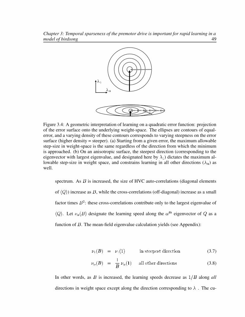
Chapter 3: Temporal sparseness of the premotor drive is important for rapid learning in amodel of birdsong 49
Figure 3.4: A geometric interpretation of learning on a quadratic error function: projectionof the error surface onto the underlying weight-space. The ellipses are contours of equal-error, and a varying density of these contours corresponds to varying steepness on the errorsurface (higher density = steeper). (a) Starting from a given error, the maximum allowablestep-size in weight-space is the same regardless of the direction from which the minimumis approached. (b) On an anisotropic surface, the steepest direction (corresponding to theeigenvector with largest eigenvalue, and designated here by
ã g ) dictates the maximum al-lowable step-size in weight space, and constrains learning in all other directions (
ã æ ) aswell.
spectrum. As � is increased, the size of HVC auto-correlations (diagonal elements
of éDá|ê ) increase as � , while the cross-correlations (off-diagonal) increase as a small
factor times � � : these cross-correlations contribute only to the largest eigenvalue oféDá|ê . Let å æ O���R designate the learning speed along the ä�ë w eigenvector of á as a
function of � . The mean-field eigenvalue calculation yields (see Appendix):
å g�O=�®Rì[ å g©OP��R íIî�ï"ð3ñ©ñ�òhñ�ïSðÚó�íIÞrñ�ô�ðríIõYî (3.7)å æ O=�®Rì[ �� å æ OP��R öV÷I÷�õVðrø�ñ©Þùó�íIÞSñ©ô�ðríIõYî�ï (3.8)
In other words, as � is increased, the learning speeds decrease as � ·V� along all
directions in weight space except along the direction corresponding toã g . The cu-

Chapter 3: Temporal sparseness of the premotor drive is important for rapid learning in amodel of birdsong 50
mulative initial error generically has significant components in several directions, so
the learning time with �ú[ � will be approximately twice as long as for �û[×� . It
is important to note, also, that the effects of increasing � on learning speed should
be visible soon after learning has begun and the first transients have passed (learning
of the first eigenvector), and not just toward the end of learning, where fine features
remain to be learned. This is in good agreement with the overall decrease in learn-
ing speeds observed in the simulations of the last section. Moreover, in the linear
analysis, the scaling of network speed with � is an essential one (see Appendix):
given a fixed network size, motif length, and HVC single-burst duration, increasing
the number of bursts per HVC neuron per motif necessarily leads to a reduction in
the optimal learning speed for the network (no adjustable parameters to remove this
dependence).
The mean-field analysis also sheds light on the identity of the eigenvector with the
largest eigenvalueã g : it is the common mode eigenvector, with all positive entries,
that corresponds to a simultaneous increase or decrease, for all parts of the motif, in
the summed drive from HVC to the motor outputs. It is intuitive that this is the most
“volatile” mode, leading to explosive growth of network activity. The remaining
modes are differential, allowing rearrangements of the motor drive from moment to
moment in the song without a large net change in the mean strength of the drive.
Numerical eigenvalue calculation. The vastly simplified mean-field derivation of
the scaling of learning speed with � (from the eigenvalues of éDá|ê ) neglected variance
and other higher-order statistics of á . To check the results of the analysis, therefore,

Chapter 3: Temporal sparseness of the premotor drive is important for rapid learning in amodel of birdsong 51
we numerically compute the eigenvalues of á from randomly generated HVC activ-
ity matrices (see Methods), withvËw
=3000, ¢ =300 ms, £¥¤ = 6 ms, and �YQ = 0.1 ms; �was varied to be �Yn � n3�n or � . The results are shown in Fig. 5, and agree well with the
mean-field analysis. In Fig. 5(a), we plot the top 300 �À[«� eigenvalues, together
with the top 300 �«[×� eigenvalues scaled by 1/8. All the eigenvalues for �«[«�form a continuum, and the scaled � [ì� eigenvalues sit on the same continuum,
except for the top eigenvalue, which is much larger than the rest. The gap between
the topmost eigenvalue and all the rest for �ü�×� is better seen in the inset of Fig.
5(a), where the largest eigenvalue scales as � � , while the second-largest scales as � .
This causes learning speeds to scale as ��·V� (Fig. 6), as derived in Eq. (3.8).
The numerical computation shows that there is some spread in the eigenvalue contin-
uum even with �Ø[�� : When HVC neurons burst once per song motif, their activities
partially overlap due to their small but non-negligible burst durations, leading to non-
zero cross-correlations between neurons and a concomitant spread in the eigenvalue
distribution; this would lead to slower learning than if bursts were completely non-
overlapping. However, increasing the number of bursts per HVC neuron leads to
further correlations in HVC activity and a considerably larger spread of eigenvalues
and thus a slower descent on the error surface.
3.5 Discussion.

Chapter 3: Temporal sparseness of the premotor drive is important for rapid learning in amodel of birdsong 52
Figure 3.5: Eigenvalues: numerical calculation to check mean-field results. The top 300eigenvalues of the correlation matrix á , divided by � , for �ý[ý� bursts per HVC neuronper song segment (Black þ ), and for �ÿ[Ø� (Grey þ ). Inset: The scaling of
ã g ( � ) andã �( � ) with � , from numerical calculations. We see that
ã gS·V���û� , whileã � ·V��� const.
Solid lines show the same scaling, derived from éDá|ê�uSummary. We have built a simplified framework to analyze the learning of premotor
representations in the songbird premotor circuit, given a sparse premotor drive from
HVC, a set of plastic connections between HVC and RA, and a gradient learning rule
that minimizes the mismatch between the tutor and pupil songs. Within this frame-
work, we have demonstrated how temporally sparse activity allows the fast learning
of premotor representations, and quantified, in a network of linear neurons, the de-
pendence of learning rate on the number of times an HVC neuron is active during
a motif. Sparsely active HVC neurons have small cross-correlations: increasing the

Chapter 3: Temporal sparseness of the premotor drive is important for rapid learning in amodel of birdsong 53
Figure 3.6: Linear analysis: learning speed as a function of � , numerical and analyticalresults. The scaling of the 1-burst-normalized learning speeds, åYæ O=�®Rr· å�æ O"��R vs �an is shownfor modes äÿ[ � ( � ) and ä [ � �Y� (). These values are obtained from the numericalcalculation of the eigenvalues of á . Solid line: the predicted scaling of learning speed with� for all ä �^� , from the mean-field correlation matrix é�áËê .
number of HVC bursts per motif increases cross-correlations in HVC activity, which
leads to correlated changes of synaptic weights. To keep network activity from di-
verging due to the correlated weight changes, the maximum allowable weight-update
size must be constrained; this normalization decreases the step-size for other, uncor-
related weight changes that are required for learning. Hence, the overall learning
speed decreases with increasing numbers of HVC bursts per motif. Although our
analytical description is based on linear units, the simulations (Fig. 3) of learning in
nonlinear units and the heuristic explanation of increased synaptic interference with
increased numbers of bursts point to a broader relevance of this analysis to networks
with more realistic neurons.

Chapter 3: Temporal sparseness of the premotor drive is important for rapid learning in amodel of birdsong 54
For a similar reason, we expect these sparseness arguments to pertain to other, more
biologically plausible learning rules that act to minimize a cost function or error sig-
nal by stochastically approximating the gradient, for example, various reinforcement
learning type algorithms. In fact, the impetus to increase learning speed through
sparse coding may be considerably greater if learning proceeds through reinforce-
ment of random trials because such stochastic gradient algorithms are typically slow.
Relation to past work. Questions about training time in perceptrons have been
studied in the machine learning community, resulting in prescriptions to speed up
learning by rescaling the learning rate parameter (weight update step size) differently
along the different eigenvectors, or by re-parameterizing neuronal activities to make
the error surface more isotropic. In a closely related work to this one, LeCun et al.
[52] in particular recommend that the eigenvector associated with the largest eigen-
value be subtracted from the learning updates, or that symmetrically activeÛ �|�Vn¥�VÜ
units be used in the input layer instead ofÛ ��n¥�VÜ units, to reduce the mean of the off-
diagonal entries of the input correlation matrix and hence reduce the anisotropy of
the error surface by reducing the distance between the largest and remaining eigen-
values. Since neural firing rates are zero or positive, units in biological networks are
necessarily asymmetric. Furthermore, although the learning rate parameter (overall
step size) may easily be set at the individual synaptic level, it is not obvious how
to apply separate learning rates to separate eigenvectors, since individual synapses
participate in multiple eigenvectors. However, we suggest that with the use of unary
HVC activity, biology may have found its own solution to these very problems in the

Chapter 3: Temporal sparseness of the premotor drive is important for rapid learning in amodel of birdsong 55
case of birdsong learning.
Juvenile HVC activity. Single-unit HVC recordings have only been made in adult
birds, where the coding is seen to be unary. We wondered what the role of such
sparseness in HVC might be, and found that it could confer a great advantage in
terms of learning speed if present during the learning process. On this basis, we
predict that the sparseness of HVC activity may be integral to the learning process
and should thus already be present in the HVC of juvenile birds instead of arising as
an emergent property late in song learning.
Other implications of sparse coding. The arguments presented here add to an exist-
ing body of theoretical work arguing for the importance of sparse codes for learning
in various neural systems. It is well established that for sequence generation in re-
current networks, relatively sparse activity allows for the reliable storage of longer
sequences (higher capacity) [41, 42, 43, 44]; however, the role of HVC in the gener-
ation of sequences, and hence the relevance of these findings to the birdsong motor
circuit, remains unclear. Temporally sparse coding could also help with the problem
of temporal credit assignment in learning, encountered when feedback about a per-
formance arrives significantly later than the neural activities that generated it. Sparse
HVC activity could reduce the potential for incorrect associations of multiple bursts
of neural activity with an error signal generated by just one of the bursts. Finally,
HVC may play an important role not just in motor aspects of birdsong learning and
production but in song recognition as well [53, 54, 55, 56], and sparse coding could
be an asset for such capabilities in ways not discussed in this work.

Chapter 3: Temporal sparseness of the premotor drive is important for rapid learning in amodel of birdsong 56
3.6 Appendix
Learning curve With linear RA neurons, we define the network equations to beTo[ L N nµWo[ M L N�� �ÒN n whereN
is thev|w�� v ¼ matrix of HVC activity,T is the
vxy��v ¼ matrix of RA activity, W is avË{��v ¼ matrix of output activity,M is the matrix of fixed weights from RA to the outputs, and L is the matrix of
plastic weights from HVC to RA.v ¼ [ ¢Ì·V�YQ is the number of discrete time bins
in the motif, where ¢ is the motif length and ��Q is the grain size. With a change
of variables á � NcN � and ±�[ � � � Í , where� Í is defined by
� Í N [À� (� Í
exists if a solution exists, i.e., if the learning task is realizable), the cost-function is� [ g� ÝßÞ Û ±cáà± � Ü�u Applying a gradient descent update, Eq.(3.4), on�
, we have that±�Á OG±¿�o�ÅM M � ±cá|R , where � is a positive scalar that scales the overall learning
step size. If each RA neuron projects to one output unit, and if the summed synaptic
weights to each output are approximately equal, MsM � becomes a scalar matrix that
can be absorbed into � . Thus, the multilayer perceptron problem with two layers
of weights becomes effectively a single-layer perceptron, and we have that after �iterations ± �����µ[o± � � �3OP�Ì� ��á|R�� , so
� ����� [ �� ÝßÞ Û ± � � � OP��� ��á|R � á OP�Ì�l��á � R � ± � � � � Ü�u (3.9)
In the eigenvector basis of the Hessian matrix á (eigenvaluesÛ�ã æ ehg%��������� ` b Ü arranged
in non-increasing order,ã g���uÖu�u�� ã ` b ), with projection of the �Åë w row of ± � � � along
the ä ë w eigenvector given by �ùX æ , the error after � learning iterations is given by

Chapter 3: Temporal sparseness of the premotor drive is important for rapid learning in amodel of birdsong 57
� ����� [ ��d æ � X OP���l� ã æ R"� � ã æ � �µX æ�� � u (3.10)
Let � æ � ã æ Ð X � �µX æ�� � represent the initial error along the ä th eigenvector. The total
error evolves iteratively via multiplication of the initial errors � æ by a factor O"�Y��� ã æ R �per iteration; � must be chosen small enough so that � �z� � ã æ�� Ñ � for each ä , to
allow error to decrease and for the learning curve of Equation (3.10) to converge.
Hence, � must be less than � · ã g , and it is easy to see that the optimal choice for � is�ÅÍx[ú��· ã g ( � Ñ ��· ã g leads to over-damped convergence, while ��· ã g Ñ � Ñ � · ã gdisplays under-damped oscillatory convergence).
Analysis of eigenvalues The mean-field matrix é�áËê is formed by replacing all ele-
ments of á by their ensemble-averaged expectation values (i.e., generate á and aver-
age, element by element, over several trials). Therefore, é�áËê\[� v ¤�� ¨ O=� � v �¤ · v ¼ R! " � ,
wherev ¤ � £©¤"·���Q . There are only two distinct eigenvalues,
ã gÚ[� v ¤ ¨ � � v �¤ O vxw · v ¼ RÚ�� � v|w�v ¤�OG£©¤%· ¢sR (providedv|w £�¤P· ¢$# � ) corresponding to the common mode eigen-
vector, andã � [ � v ¤j� � � v �¤ · v ¼ � � v ¤ (provided ¢�# �x£©¤ ) corresponding to
thev|w �� differential modes. (This effect, of a continuous eigenvalue spectrum with
a single large eigenvalue, is generic for N�
N matrices with random entries of mean% on the diagonal and & on the off-diagonal, if &'# % · v [58].) Hence the learning
rate for all modes äo� � is given by å�æ [ûO"� ·V�®R©OG¢Ì· vxw £�¤"R(�×��·V� , as in Eq. (3.8),
Figure 6.

Chapter 4
A biologically plausible learning rule for
reward optimization in networks of
conductance-based spiking neurons
It is not known how animals learn to perform complex goal-oriented tasks. Behav-
ioral and neurophysiology studies as well as common experience indicate that ani-
mals can be taught to perform such tasks with the help of simple reinforcing rewards.
Numerous learning rules exist in the machine learning literature that perform reward
optimization; however, they cannot be applied to networks with biologically realis-
tic neurons interacting through voltages and conductances. In this paper we present
a biologically plausible rule for synaptic learning in recurrent networks of spiking,
voltage and conductance based neurons, that can provably optimize reward under
fairly general conditions.
58

Chapter 4: A biologically plausible learning rule for reward optimization in networks ofconductance-based spiking neurons 59
4.1 Introduction
In machine learning, since several techniques exist to perform optimization, it has
proved fruitful to transform the goal-directed learning problem into one of reward
maximization by equating closeness to the goal with reward. Some of these ap-
proaches (e.g., backpropogation) rely on the direct computation of gradients to max-
imize reward. Such direct-gradient techniques cannot be applied to neural networks
with conductance-based spiking model neurons, where, because of their rich tempo-
ral dynamics, the relevant gradients cannot be expressed explicitly. If the learning
task involves any form of motor control, reward would depend on the neural–motor
transformation; thus, learning depends on knowledge of many gradients that are im-
possible to compute explicitly. An alternative approach to this problem is stochastic
gradient ascent, where the appropriate gradients are estimated by measuring the im-
pact on the reward of perturbations in the system parameters; the learning rule moves
the system parameters along the stochastically measured local gradient. While some
concrete rules for learning by stochastic gradient computation have been formulated
and shown to perform gradient ascent, few rules have been articulated on the synap-
tic or single-neuron level that are both biologically realistic and capable of provably
performing reward optimization.
Our goal in this paper is to provide a biologically plausible and demonstrably work-
able learning rule that can optimize reward. The learning rule proposed here can be
placed in the general category of REINFORCE algorithms [49], and it applies to ar-
bitrary networks of conductance-based spiking neurons. It relies on the correlation
Chapter 4: A biologically plausible learning rule for reward optimization in networks ofconductance-based spiking neurons 60
of reward with synaptic noise and presynaptic inputs. Heuristically, the rule works in
the following way: if greater-than-average excitatory noisy synaptic input to a neu-
ron at some time correlates positively with reward, increase the excitatory synaptic
weights of all inputs to that neuron which were active at that time. Conversely, if all
lower-than-average excitatory input to a neuron at one time correlates with reward,
reduce the activity of that neuron for that time by lowering the strength of all partic-
ipating inputs to it. Thus, noisy inputs act as a source of exploration, to probe the
effects of changing neural activity on reward; the correlation information is used by
the learning rule to make changes in the network weights that reinforce patterns of
neural activity that lead to high reward, and to weaken patterns of neural activity that
lead to low reward.
In the next section, we present the formal learning rule; in sections two and three, we
prove in a network of recurrently connected excitatory conductance based neurons
that learning follows the gradient of the expected reward, and in section four we gen-
eralize the learning rule to apply in networks with excitatory and inhibitory neurons,
as well as in networks with noisy currents instead of noisy conductance inputs.
4.2 Learning rule
We consider learning in a system with three central elements: a recurrent network
of spiking neurons, a noise generator that perturbs the activities of the neurons in
the recurrent network, and an evaluator that provides a reward signal ) based on the
network output.

Chapter 4: A biologically plausible learning rule for reward optimization in networks ofconductance-based spiking neurons 61
The prescribed learning rule is given by
� L �(UÌ[��*) � �� �YQèO,+��POGQSR��²é-+©�tOZQSRSê3R�¾.U OZQSR$u (4.1)
L �(U is the weight of the �/. } synapse from neuron } to neuron � , and � is a positive
scalar learning rate parameter. Learning updates are made following each episode
of network activity that lasts from time � to ¢ . The reward ) is some functional
of the neural activities that occurred in this interval. Each neuron in the network
receives, in addition to feedforward or recurrent synaptic inputs from the rest of the
network, a time-dependent noise input, + �%OZQSR . Neural activity is characterized by
neural voltages, 0q�POGQSR�n synaptic activations ¾ �%OZQSR resulting from presynaptic spikes,
and synaptic conductances, 1V�POGQSR . The dynamics of these variables are summarized
in the following equations:
¾©�POGQSR¬[ ] ¼ 2 0½OGQ%� R$n$¾�OZQ%� R43cQ%� Ñ Q65 (4.2)1 �POGQSR¬[ d U L �(U�¾$U OGQSR ¨ &3�POZQSR ¨ +©�%OZQSR � 1���� 768 ë OZQSR ¨ +©�%OZQSR (4.3)�90��POGQSR�YQ [ �:1<; 2 0q�%OZQSR��=0�;>5Ì�?1 �POZQSR 2 0q�%OZQSR��=0�@A5 � d æ 1 æ� OGQSR 2 0q�%OZQSR��B0 æ 5(4.4)� 0��I� 7�8 ë �?+©�tOZQSR 2 0q�%OZQSR��=0�@C5 (4.5)
Dynamic variables without a subscript are vectors that represent the state of all neu-
rons in the network at time Q : for example, 0½OZQSRÉ[ Û 0µg©OGQSR�n¥uÖu�uÖnD0 N OZQSR.Ü is the vec-
tor of neural voltages at Q . Variables with no subscript and no time index are ma-
trices that represent the states of all neurons for all times in an episode, so that

Chapter 4: A biologically plausible learning rule for reward optimization in networks ofconductance-based spiking neurons 62+|[ Û +��%OGQSR � ��[ � v nSQ�E�Ã(��nr¢ÌÆ=Ü�u
Equations (4.2– 4.4) are quite general and can be used to describe the dynamics of
various conductance-based neurons, including Hodgkin–Huxley and integrate-and-
fire models. The voltage equation includes contributions from an intrinsic neural leak
conductance, 1F; , synaptic input conductances, 1V� , and fast non-linear ion-channel
conductances, 1 æ� , responsible for spiking dynamics.
The goal of learning is to maximize reward; the learning rule proposed above does
this by collecting information, via the correlation of stochastic inputs with reward,
on how reward depends on network parameters. More simply, if greater than average
excitatory noise input to a neuron leads to a large reward, increase the weights of all
recently active synaptic inputs to that neuron. On the other hand, if lower than aver-
age excitatory noise input to a neuron leads to a large reward, decrease the weights of
all recently active inputs to than neuron. While the weight updates improve the aver-
age performance of the network, the weight change of an individual synapse in one
trial is stochastic, though slightly biased in the direction of improving performance.
From this description, it seems like the learning rule is hill-climbing on the reward
surface, but to guarantee this property in arbitrary networks would require a proof.
Here, we prove that the learning rule of Equation (4.1) performs stochastic gradient
ascent on the reward in arbitrary networks of spiking neurons, under the following
conditions:
– If the noise + is Gaussian, we prove, for arbitrary networks, that the learning
rule performs stochastic gradient ascent on the reward.
Chapter 4: A biologically plausible learning rule for reward optimization in networks ofconductance-based spiking neurons 63
– More generally, for arbitrary, spatially and temporally uncorrelated noise + �POGQSR ,we prove within a linear approximation that the learning rule performs stochas-
tic gradient ascent on the reward. We show that this is still true if the injected
noise has some temporal correlation.
4.3 Arbitrary noise
Our strategy in this section is to start with the stated learning rule, Equation (4.1),
and average over noise to derive the expected weight change. With some linearization
and algebraic manipulation, we see that the expected weight change is proportional
to the gradient of the noise-averaged reward.
Let the network dynamics be given by Equations (4.2–4.4). We assume that the noise
inputs +©�POZQSR are random variables drawn from an arbitrary distribution or process, but
are spatially uncorrelated; that is, OG+ �tOZQSR � é-+��POGQSRrê3R�O,+.U OGQSRÕ� é-+.U OGQSRrê3R|[IH$�(UKJ�OZQè� QSR ,where J is a normalized correlation function, Ï J�OZ£qRS�Y£ [ � . For example, +©�POGQSRcould be the synaptic activation of a neuron firing a poisson spike train. In this case,
since + is derived by temporally filtering a neural spike train, it would have clear
temporal correlations.
Let é ê represent noise-averages over + . The expected weight update is
é � L �(U�ê¬[ � �F+MLßO,+�RN") � �� �YQ 2 + ë� �oé-+ ë� êO5̾ ë�(UKP (4.6)
[ � �� �YQ � �Q+MLßOG+�R � ë�(U 2 + ë� �²é-+ ë� ê 5 n (4.7)
Chapter 4: A biologically plausible learning rule for reward optimization in networks ofconductance-based spiking neurons 64
where we have defined� ë�(U � )z¾©ë�(U u Note that
� ë�(U is a functional of + . Taylor expand-
ing� ë�(U ÃR+�Æ to first order around é-+�ê , the average weight update becomes
é � L �(U�ê¬[ � �� �YQq�û�F+MLßO,+�RTS � ë�(U Ã�é-+�ê"Æ ¨ d X �ú�YQ%� H � ë�(U ÃÖé-+�ê%ÆHU& ëWVX 2 + ë VX �oé-+ ë VX êX5�Y 2 + ë� �²é-+ ë� êO5[ � �� � �� �YQ"��Q%� H � ë��U ÃÖé-+�ê%ÆHU& ëWV� J�OGQ�� Q%�fR (4.8)
� � �� � �� �YQ"��Q%� H�é � ë�(U êHU& ë V� J�OZQ�� Q%�ÖR�u (4.9)
The last line follows from the expression above it only within a linear approximation,
i.e., if� ë�(U depends linearly on +�u
Temporally uncorrelated noise. If + is temporally uncorrelated so that J�OZQß� Q � RÚ[HÅOZQù� Q � R$n we see that
é � L¿��U�ê [ � �� �YQ HHZ& ë� é�)o¾ ë�(U ê (4.10)
[ � é�)zê� L �(U u (4.11)
Equation (4.11) follows from direct application of the sensitivity lemma (Lemma
2). So, in the special case of spatially and temporally uncorrelated noise injections,
we have proved that the learning rule on average performs gradient ascent on the
expected reward.
Temporally correlated noise. If + is temporally correlated, J�OGQ2� Q � RT[[\HÅOZQ2��Q � RK]defining é � ë�(U ê � ]jOZQSR and making the change of variable £½[oQ�� Q � n

Chapter 4: A biologically plausible learning rule for reward optimization in networks ofconductance-based spiking neurons 65
é � L �(U�ê¬[ � �� �YQ%� HHU& ë V� � ��£®]jOZQ%� ¨ £ÎR^J�OG£ÎR$u (4.12)
J is an autocorrelation function, so it peaks at £�[ú� and is symmetric. Thus, Jwindows ] , the function in the integrand, around £ [À� ; if correlations are short,J decays rapidly away from £ [ÿ� , and the window is narrow. We Taylor expand]jOGQ � ¨ £qR about £ [��n and change notation so that Q � Á�Q , to get
é � L �(U�êì[ � �� ��Q HHU& ë� � �Y£`_2]�OZQSR ¨ � ]� £aaaacb e � £ ¨ �� � � ]� £ � aaaa�b e � £��QdeJ�OZ£ÎR (4.13)
[ ���� ��Q H�]jOGQSRHU& ë� ¨ £ �� ���� �YQ HV] � � OZQSRHZ& ë� u (4.14)
We assume J is normalized, Ï �Y£fJ�OG£ÎRË[À� ; the term involving Ï ��£gJ�OZ£qRP£ van-
ishes because J is symmetric. The constants £ � � Ï �Y£s£ � J�OZ£qR reflect the temporal
characteristics of the noise + (say for example that + has correlations on the time-scale
of ¢ih , with autocorrelation function J�OZ£qR2[ g�Kj ¸ ¹ik b k » �Kj ] then £ � reflects this informa-
tion, because £ � [ � ¢ �h ). Substituting ]jOZQSRz[Àé � ë�(U ê|[«é�)z¾ ëU ê�n we see at once that,
like Equation (4.10), the first term of equation (4.14) is the gradient of the expected
reward:
é � L �(U©ê\[ � é�)zê� L �(U ¨ £ �� � �� �YQ HHU& ë� � � él)z¾ ëU ê� Q � (4.15)
The second term reflects deviations, due to temporal correlations in the injected
noise, from the true gradient. Thus, for the weight updates to approximately follow

Chapter 4: A biologically plausible learning rule for reward optimization in networks ofconductance-based spiking neurons 66
the gradient of the reward, the second (non-gradient) term should be much smaller
than the first (gradient) term. We see from Equation (4.14) that for this to be true, it
is sufficient (but not necessary) to have ] � � OZQSR bnm� ç ]jOZQSR�3cQ , or in other words,
�£ � # o m6prq ¼-stvuo ë m� é�)z¾ ëU ê u (4.16)
This expression provides bounds within which, even if correlations are present in
the injected noise, deviations of the weight update away from the gradient of the
expected reward can be neglected. If the condition in Equation (4.16) is satisfied, we
have once again proved that the learning rule on average performs gradient ascent on
the expected reward.
4.4 Gaussian noise
In this section we show, without a linear approximation, that if the noise + is gaussian,
learning proceeds by stochastic gradient ascent on the expected reward. Our strategy
is to compute the expected, or noise-averaged reward, and use the gradient of this
expression to derive a weight update rule, which we show is proportional to our
proposed learning rule of Equation (4.1).
To perform gradient following, a stochastic learning rule must obey

Chapter 4: A biologically plausible learning rule for reward optimization in networks ofconductance-based spiking neurons 67
é � L �(U©ê\[ý� é�)zê� L �(U [ �� L �(U d w � x )ªÃ�0zÆ?ÇaO,1cnD0xR (4.17)
[ d w � x )ªÃy0xÆ �� L �(U Ç OG1hnn0|R (4.18)
[ é�)¦� ÷IõFz\Ç� L¿��U ê�u (4.19)
Learning rules of the form� L�(U�[{) o*|R}�~Z�oK�e� t will clearly satisfy the condition above,
and belong to the general category of REINFORCE [49] stochastic gradient algo-
rithms. To explicitly formulate such a learning rule, we must compute � ÷�õFz2Ç · � L �(Ufor our network.
We assume that the network dynamics are as given in Eqs. (4.2 –4.4). Since + �POGQSR are
spatially and temporally uncorrelated, and are uncorrelated with the network state,
we can decompose ÷�õFz2Ç OG1cnD0|R into a sum of the conditional probabilities over dif-
ferent neurons and past times:
÷�õFz2Ç OG1hnn0|RÚ[ `d �fehg �d ë e � ÷�õFz\Ç OG1��%OZQSRD]D0q�tOZQSR � 0½OGQ%� R$nO1 OZQ%� R$nrQ%� Ñ QSR$u (4.20)
Using the definitions of 1��I� 7�8 ë OGQSR�nD0��I� 7�8 ë OZQSR in Equations (4.3) and (4.5), we may rewrite
the above as ÷�õFz\ÇaO,1cnD0xR�[�Ð `� ehg Ð � ë e � ÷�õFz2Ç OG1��tOZQSR$nD0��POZQSR � 1 �I� 7�8 ë OGQSR�nD0��I� 7�8 ë OZQSRSR�u Since
the difference between 0Î�%OZQSR and 0q��� 768 ë OZQSR is +©�POGQSR 2 0��POZQSR��f0�@A5 , the log-probability be-
comes ÷IõFz2ÇaO,1cnD0xRÚ[^Ð `� ehg Ð � ë e � ÷�õFz\Ç 2 +��POGQSR2[ � x � � ë � ¹ x ��� ��� s � ë �x � � ë � ¹ xD� aa 0q�I� 7�8 ë OZQSR 5 u Therefore,

Chapter 4: A biologically plausible learning rule for reward optimization in networks ofconductance-based spiking neurons 68
� ÷�õFz2Ç� L¿�(U [ � �YQ HHVL ë�(U N d X�� � ÷�õFz2Ç 2 +©XYO,� RÚ[È� 0qX�O,� Rß�=0ÎX�� 7�8 ë O-�hR0qXYO,�hR��B0"@ aa 0qX�� 7�8 ë O,� R 5 P[ � �YQ 2 ÷IõFz\ÇaO,+©XYO,� RSR 5 � �0ÎXYO-�hRù�=0�@ H<0qX�� 7�8 ë O-�hRHVL ë�(U (4.21)
[ �� �h �û�YQ 2 +©�tOZQSRj�oé-+��POZQSRSêO5̾.UVOGQSR (4.22)
where the last line follows because + is Gaussian distributed, and because HZ0 X�� 768 ë O-�hR"·<H�L^ë�(U [H$�fX�H ë � 2 0��POGQSRh��0�@C5 ¾.U�OZQSR . Therefore, learning will follow the gradient of the expected
reward if the update rule is
� L �(UÌ[�)¦� ÷IõFz\Ç� L¿��U [$) � �� �YQ 2 +©�%OZQSRj�oé-+��POZQSRSê 5 ¾.UVOGQSR�u (4.23)
This the stated learning rule of Equation (4.1), completing the proof that with Gaus-
sian noise inputs in an arbitrary recurrent network of conductance based neurons, the
learning rule performs stochastic gradient ascent on the reward.
4.5 Generalization of the learning rule
Here we describe how learning is modified if the network contains both excitatory
and inhibitory neurons, or if noise enters through currents instead of through con-
ductances. The proofs are straightforward, as they closely follow the derivations
provided above.
Chapter 4: A biologically plausible learning rule for reward optimization in networks ofconductance-based spiking neurons 69
4.5.1 Learning with excitatory and inhibitory conductances
In general, neural networks contain both excitatory and inhibitory neurons, and it is
thought that inhibitory connections may also be plastic. Furthermore, the synaptic
noise inputs could also be excitatory or inhibitory. We generalize the learning rule of
Equation (4.1) so it applies to networks with excitatory and inhibitory neurons.
The new learning rule is essentially the same as Equation (4.1), but modified by a� � constant prefactor, that dictates the sign of synaptic change based on the reversal
potentials of the presynaptic input and the noise:
� L �(UÌ[��<ht��� UK) ���� �YQèO,+©�%OZQSR��²é-+��GêrRr¾.U OZQSR�u (4.24)
The constant �Fht��[ì� if the noise synapse to neuron � is excitatory, and is �x� if it
is inhibitory; similarly, � UË[°� if the presynaptic input from neuron } is excitatory,
and is -1 if it is inhibitory. This learning rule performs hill-climbing on the reward
function. In other words, the prescribed weight updates drive the network toward
nondecreasing reward, in a direction that is always within 90 degrees of the true
gradient of the expected reward.
To prove this, we rewrite Equations (4.3–4.4) to include both types of conductances:

Chapter 4: A biologically plausible learning rule for reward optimization in networks ofconductance-based spiking neurons 70
¾©�POGQSRì[ ] ¼ 2 0½OZQ%�fR�n$¾�OGQ%� R�3cQ%� Ñ Q65 (4.25)1 @�I� 7�8 ë OGQSRì[ dUD��@ L¿��U©¾.U�OZQSR ¨ & @� OGQSR (4.26)19��I� 7�8 ë OGQSRì[ d UD� � L¿��U©¾.U�OZQSR ¨ &n�� OGQSR (4.27)�*0��POGQSR�YQ [ ��1Z; 2 0��POGQSR��=0"; 5 ��1 @� OZQSR 2 0��POGQSR��=0"@ 5 �?19�� OZQSR 2 0��POGQSR��=0 � 5 � d æ 1 æ� OZQSR 2 0q�%OZQSR��=0 æ 5where 1 @� OGQSRÕ[�1 @�I� 7�8 ë OGQSR ¨ +©�%OZQSR and 1 �� OGQSRè[�1 ��I� 7�8 ë OGQSR if the noise injected into neuron� is excitatory ( 0�hr� y 8l� [�0 � ); conversely, 1 @� OGQSR2[�1 @�I� 7�8 ë OZQSR and 1 �� OZQSR\[$1 ��I� 7�8 ë OGQSR ¨ +��POGQSRif the noise injected into neuron � is excitatory ( 0ihr� y 8l�Ò[�0�@ ). Closely following
the derivation of Section 4.4, the learning rule for stochastic gradient ascent on the
reward becomes:
� L¿�(U [�) � �� �YQ 2 0�U"� y 8-�2�=0q�%OZQù� � QSR652 0ghr� y 8l�è�=0��POZQù� � QSRX5 O,+��%OGQSRj�oé-+©�Gê3Rr¾.U OZQSR$u (4.28)
where 0�U"� y 8l�(E Û 0 � nn0"@�Ü , depending on whether the presynaptic neuron } is inhibitory
or excitatory. We notice that the signs of2 0ghr� y 8-�Y��0��"OZQ©� � QSR 5 and
2 0�UP� y 8l�V��0q�"OGQ¥� � QSR 5stay the same at all times, because 0 � § 0 OZQSR § 0�@ at all times. Thus, Equation
(4.28) differs from the learning rule of Equation (4.24) by a factor of aa x t � p ��� ¹ x � � ë ¹9� ë � aaaa x j � p ��� ¹ x � � ë ¹9� ë � aamultiplied into the eligibility at each time step. Since the stated learning rule differs
from the expression for stochastic gradient ascent on the reward only by multipli-
cation of a positive vector, it follows that the learning rule of Equation (4.24), for
networks with excitatory and inhibitory conductances, stays within 90 degrees of the
gradient, and consequently performs hill-climbing on the reward.

Chapter 4: A biologically plausible learning rule for reward optimization in networks ofconductance-based spiking neurons 71
4.5.2 Noise in currents
If the postsynaptic neuron is perturbed by noisy currents instead of conductances,
the expression to move along the reward gradient is slightly modified to include a
postsynaptic voltage dependence,
� L �(UÌ[�) � �� �YQ 2 0�U"� y 8-�2�=0q�%OZQù� � QSR 5 O,+©�%OZQSR��²é-+��GêrRr¾.U OZQSR�u (4.29)
In analogy with previous section, we define the actual learning rule to be:
� L �(UÌ[�� UD) � �� �YQ 2 +©�%OZQSR��²é-+��Gê 5 ¾.U OZQSR$u (4.30)
Once again, this learning rule drives the network uphill on the reward surface, always
within 90 degrees of the gradient.
4.6 Discussion
In summary, we have proposed a synaptic learning rule for recurrent networks of
voltage and conductance based spiking neurons that demonstrably performs stochas-
tic gradient ascent on a reward function. Synapses are only required to maintain
a local eligibility trace of recent past local activity; plasticity in these synapses is
governed by the product of this local eligibility trace with a global reward signal.
Another quality of this learning rule is that it is able to weather complex, short time-
scale dynamics such as facilitation and depression in synapses; learning still provably
follows the gradient of the reward.

Chapter 4: A biologically plausible learning rule for reward optimization in networks ofconductance-based spiking neurons 72
The form of the proposed learning rule makes it possible to generate specific pre-
dictions for neurophysiology. There are two conditions for synaptic change to take
place: (1) the presynaptic neuron must have been recently active; (2) presynaptic
neural activity must be followed by reward. The sign of synaptic change is instructed
by the noise synapse onto the postsynaptic neuron: if the noise input to the postsy-
naptic neuron was active at the time of the presynaptic input, then the synaptic weight
would increase. On the other hand, quiescence of the postsynaptic noise input at the
time of the presynaptic input, if followed by reward, would lead to a decrease in the
synaptic weight. Thus, to gain a direct handle on plasticity, the synaptic physiolo-
gist would need to identify the reward signal, and be able to independently control
activity in the presynaptic neuron and the postsynaptic noise input.
This learning rule requires the confluence of three signals at the postsynaptic neuron:
presynaptic input, a unique noise input, and reward. The cerebellum, with convergent
circuitry from climbing fibers and parallel fibers onto Purkinje cells, is suggestive of
such a confluence. Climbing fibers are traditionally thought to convey error signals
from the inferior olive to the Purkinje cells, while parallel fibers undergo plasticity;
however, it is possible the role of climbing fibers is noise injection, not error trans-
mission. Similarly convergent circuitry is found in the song-related premotor area
RA of songbirds. RA receives inputs from two brain areas, HVC and LMAN. HVC–
RA synapses are crucial for song production and thought to be plastic, while the
LMAN–RA synapse is necessary for songlearning, but not for song production. It
would be interesting to reexamine data on cerebellar and songbird area RA plasticity

Chapter 4: A biologically plausible learning rule for reward optimization in networks ofconductance-based spiking neurons 73
from the point of view of this learning rule.
Perturbative network learning depends on the correlation of noise with reward. Typ-
ically, stochastic gradient rules extract this correlation from the product of reward
with an eligibility trace that has zero mean. If the estimation of the average noise
is biased, the eligibility ceases to have zero mean, and the product of reward with
eligibility drives learning in a biased direction, away from the gradient of the reward.
If the bias is large compared to the size of the correlations between synaptic noise
and reward, the network can go seriously astray. The learning rule proposed in this
paper is subject to the same requirement as other stochastic gradient rules, that the
subtraction of the mean noise be accurate. In this regard, the learning rule proposed
here has a distinct advantage over two recently proposed noise-based gradient rules
for biological neural networks [31, ?], because the noise inputs in our model are dis-
tinct from the network being trained, and hence are uninfluenced by the dynamics of
the network or by the changing network parameters. For this reason, it is possible for
an individual neuron to maintain a stochastic but unbiased estimate of its input noise
by locally time-averaging the noise input. In contrast, the noise variable is the plas-
tic variable in the model of [31] and thus its mean could be changing systematically
with learning; in the model of [?], the noisy variable is the postsynaptic neural spike
train, which can vary on fast time scales due to ongoing network dynamics or time-
varying non-noise inputs; thus, attempts to compute the noise by time-averaging in
these models could be problematic and lead to biased estimates of the noise.
Mathematically, this learning rule is analogous to node perturbation. In fact, if

Chapter 4: A biologically plausible learning rule for reward optimization in networks ofconductance-based spiking neurons 74
adapted to linear, rate based units, it becomes exactly node perturbation. A common
criticism leveled at learning rules based on the correlation of noise with reward is that
since these correlations are small in large networks, the learning time increases with
increasing network size. Potentially, the learning time for a demanding task whose
complexity scales up with network size, could grow asv
, the number of neurons
receiving independent noise inputs. In comparison, learning rules similar to weight-
perturbation would scale up withv � , where
v � is the total number of plastic
synapses in the network [59]. Not all tasks scale up in complexity with network size,
however. In fact, many artificial neural network problems have been shown with
principal components analysis to depend on the learning of only a few modes, and
we show in certain biological problems, such as birdsong acquisition, that learning
time with stochastic gradient rules can be quite fast, and independent of the size of
hidden layers in the network [Fiete and Seung, unpublished].
We showed conditions under which temporal correlations in the injected noise will
and will not affect the ability of the learning rule to perform gradient ascent on the
reward. Intuitively, temporal correlations in the noise will not adversely affect learn-
ing if the task itself has broad, or slowly varying, temporal characteristics, compared
to the correlation time of the noise. For the same reasons, we expect that patterns
of spatial correlation in the noise should not adversely affect learning if the task can
be learned if the groups of neurons receiving correlated input become correlated in
activity. For example, if a group of neurons sends convergent projections to a single
output unit, it would not affect the learning task adversely if all neurons in the group

Chapter 4: A biologically plausible learning rule for reward optimization in networks ofconductance-based spiking neurons 75
received correlated noise. In general, however, it is possible for the network task to
be demanding enough so that individual neural activities have to be learned precisely,
and in this case spatially correlated noise would slow down or even prevent learning.
Finally, there is no reason for the noise statistics to be constant: it is possible to
imagine that the particular noise statistics and spatial and temporal noise correlations
could themselves be learned and could be adapted to increase the learning speed,
depending on the task that needs to be learned. If noise adapts on a slow time scale,
that would still allow for baseline noise estimation by time-averaging, and could also
speed up learning. What tasks would benefit from the adaptation of noise statistics,
and from the introduction of noise correlations, remains an open question for future
study. In general, much work remains to be done in the study of ‘meta-learning, the
designing of networks that can learn how to learn.
Another set of open questions for future work has to do with exploring the mathe-
matical relationship between seemingly different learning rules, for example, might
there be a regime where noise-based reinforcement learning is analogous to a more
traditional Hebbian or spike-time dependent learning algorithm? Hebbian learning
rules, even when gated by reward, have not been shown to provably perform reward
optimization. If some Hebbian-like rules are empirically found to be able to perform
such reward-driven learning in particular networks, then the mathematical gateway
for proving reward optimization might be through proving equivalence with this or
other existing stochastic gradient descent rules.

Chapter 5
Rapid learning of birdsong by reinforcement
of variation in spiking networks
5.1 Abstract
The adage that “practice makes perfect” refers to the gradual learning of complex
skills through an iterative process of trial, error, and improvement. Here we hypoth-
esize that such behavioral learning is based on blind variation, in the form of noisy
neural inputs, and selective reward-based modification, guided by the correlation of
the noise inputs with a global reinforcement signal. The proposed rule is an example
of stochastic gradient learning, which is often criticized as too slow to be biologically
plausible. We demonstrate that, contrary to conventional wisdom, the learning time
in a test case of birdsong acquisition in a spiking network model with delayed reward
is fast enough to be compatible with that of real zebra finches. This is because learn-
ing time scales up with the complexity of the task to be learned, and not with the size
76

Chapter 5: Rapid learning of birdsong by reinforcement of variation in spiking networks77
of the network; since the information content of song is reasonably small, learning
proceeds rapidly. Our results suggest that stochastic gradient learning can, in at least
some contexts, be fast enough to be taken seriously as a biological mechanism.
At the abstract level, our model of motor learning involves interactions between three
component subsystems: a pattern generator, an evaluator, and a noise injector (Figure
1a). The pattern generator produces motor output that, due to input from the noise
injector, fluctuates from trial to trial. When the evaluator rates the output as better
than average, the pattern generator receives positive reinforcement, making that out-
put more likely to occur in the future. By this process of trial and error, the average
performance, as measured by the evaluator, improves over time. The goal of this
paper is to make the preceding abstract model, standard in the field of reinforcement
learning [60, 28, 49], relevant to neurobiology.
At the neural level, our model contains a pattern generator that is a network of
integrate-and-fire neurons. Each neuron receives a single noise synapse, in addition
to regular synapses from other neurons in the pattern generator (Figure 1b). Each
noise synapse is driven by a random spike train from a corresponding neuron in the
noise injector. All regular synapses are assumed to receive a global reinforcement
signal from the evaluator. The present work takes the noise and reinforcement sig-
nals as given, and focuses on the question of how the pattern generator uses these
two signals to iteratively improve its performance over repeated trials.
We propose that this is accomplished by a synaptic learning rule that is driven by the
correlation between presynaptic spiking, local noise, and the global reinforcement

Chapter 5: Rapid learning of birdsong by reinforcement of variation in spiking networks78
signal (Figure 1c). When followed by reinforcement, the noise is treated as a teaching
signal that instructs active synapses to change. Positive (negative) noise, if followed
by reinforcement leads to the strengthening (weakening) of active synapses. Put
another way, if greater than expected activity of a neuron leads to reward, the learning
rule raises the activity of that neuron and hence increases the expected reward by
strengthening inputs to that neuron. Similarly, if lower-than-expected neural activity
correlates with reward, this would lead to the weakening of synapses to that neuron.
Due to the rudimentary, correlation-based nature of this synaptic learning rule, in-
dividual neurons do not require or receive information, except what is conveyed in
the single global reward signal, about downstream network activity and connectivity
or about the transformations from neural activity to physical motor output to reward.
This rule is similar in concept to learning by “node perturbation” [61, 60], and more
distantly related to “weight perturbation” and other stochastic gradient learning rules
for artificial neural networks [28]. In detail, the present rule is novel because it is
applicable to biophysically realistic voltage and conductance based model neurons.
Although noise followed by reinforcement is treated as an instructive signal, the in-
struction is in the correct direction only on average; often the prescribed change is
in the “wrong” direction for individual synapses. In fact, in a network that contains
hundreds or thousands (v h ) of noisy variables, the correlation of reward with any
one independently fluctuating variable is small ( �Ø��· v h ); to measure this correlation
accurately would require averaging over a large number ( � v h ) of iterations.
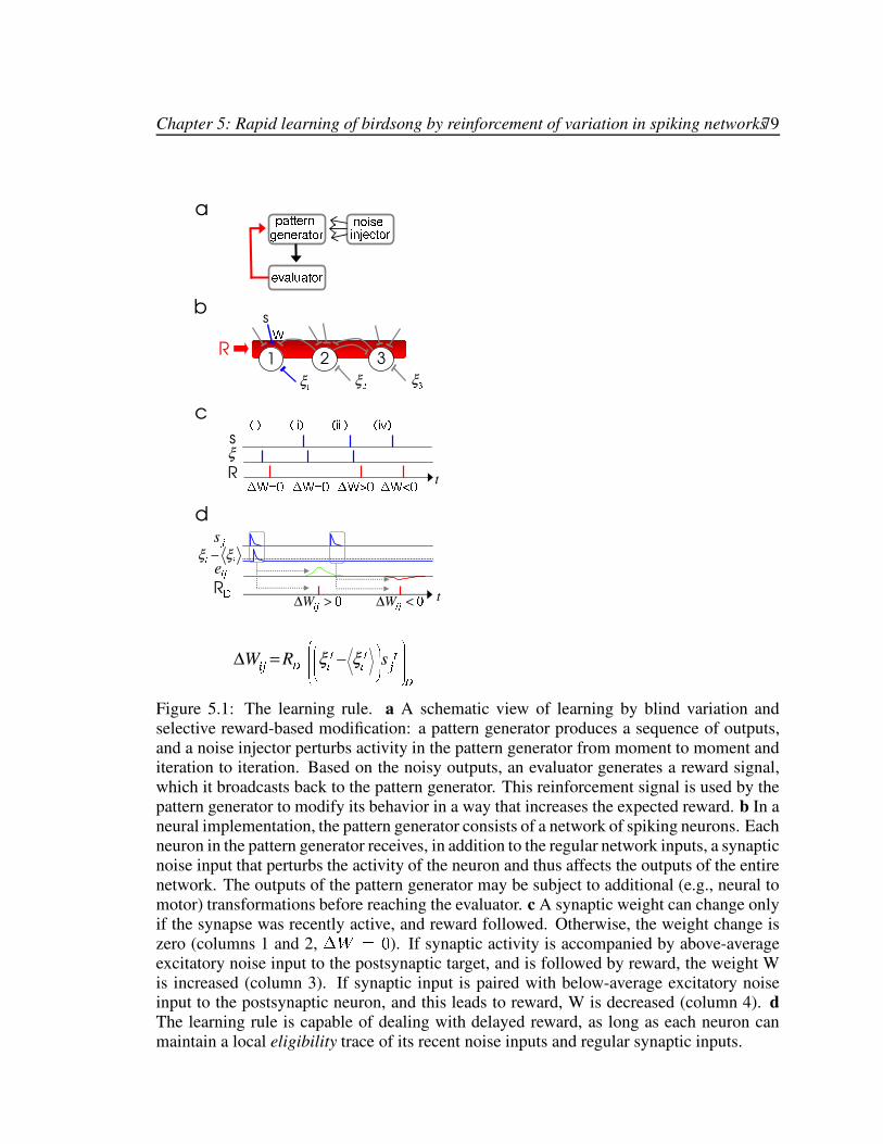
Chapter 5: Rapid learning of birdsong by reinforcement of variation in spiking networks79
Figure 5.1: The learning rule. a A schematic view of learning by blind variation andselective reward-based modification: a pattern generator produces a sequence of outputs,and a noise injector perturbs activity in the pattern generator from moment to moment anditeration to iteration. Based on the noisy outputs, an evaluator generates a reward signal,which it broadcasts back to the pattern generator. This reinforcement signal is used by thepattern generator to modify its behavior in a way that increases the expected reward. b In aneural implementation, the pattern generator consists of a network of spiking neurons. Eachneuron in the pattern generator receives, in addition to the regular network inputs, a synapticnoise input that perturbs the activity of the neuron and thus affects the outputs of the entirenetwork. The outputs of the pattern generator may be subject to additional (e.g., neural tomotor) transformations before reaching the evaluator. c A synaptic weight can change onlyif the synapse was recently active, and reward followed. Otherwise, the weight change iszero (columns 1 and 2,
� L [ý� ). If synaptic activity is accompanied by above-averageexcitatory noise input to the postsynaptic target, and is followed by reward, the weight Wis increased (column 3). If synaptic input is paired with below-average excitatory noiseinput to the postsynaptic neuron, and this leads to reward, W is decreased (column 4). dThe learning rule is capable of dealing with delayed reward, as long as each neuron canmaintain a local eligibility trace of its recent noise inputs and regular synaptic inputs.

Chapter 5: Rapid learning of birdsong by reinforcement of variation in spiking networks80
Since the learning process is based on such correlations, convergence in large net-
works may be very slow. This is a potential weakness of all stochastic gradient
learning rules.
To test biological plausibility and see whether learning can take place in a time con-
sistent with that observed experimentally, therefore, it is essential to apply these
learning rules to specific biological examples. Imitative song learning in birds is
an easily quantified but ethologically rich behavior [62, 63] that has been amply cat-
aloged throughout the learning process, which includes periods of gradual, practice-
driven improvement; in addition, detailed results on the anatomy and physiology of
song-related premotor areas are available in the literature [46]. This makes birdsong
acquisition an excellent candidate system for the analysis of motor learning.
We implement a model birdsong network to study the speed with which a noise-based
rule can drive learning in a biological system; to this end, we incorporate impor-
tant biological details, such as the architecture of and neural activity in the songbird
premotor circuit. However, we do not attempt to provide an exact model of the en-
tire song system, since important details about acoustic production, song preference,
comparison, and reward evaluation, are unknown. It is likely that, due to evolution-
ary adaptation, the bird brain uses a convenient perceptual metric for the assessment
of reward; this and other adaptive features would serve to make learning easier. For
example, two sounds with a factor of two difference in pitch may be perceptually
closer than two sounds separated in pitch by a factor of just 1.5. This, together with
the period-doubling ability of the syrinx [64], could give rise to some of the interest-

Chapter 5: Rapid learning of birdsong by reinforcement of variation in spiking networks81
ing features seen in the song-learning trajectory of actual zebra finches [65]. Because
finch songs are not of the pure-tone variety, but contain multiple harmonics, such a
perceptual metric could be an adaptive feature to aid learning. Since our aim is to
show that learning can be fast enough with a simple stochastic gradient rule, omitting
details that could facilitate learning ought not to detract from the demonstration, but
bolster it.
The work of Doya and Sejnowski provides an ideal starting point for this portion
of our study [47]. They have suggested that the abstract model of Figure 1a can be
mapped onto avian brain anatomy. The pattern generator corresponds to the premo-
tor nuclei HVC and RA, the motor neurons, and the vocal and respiratory organs.
Avian brain nucleus RA is a candidate area in which our synaptic learning rule might
operate. RA is important for song generation, because it drives the motor neurons
that control vocalization. It receives input from two prominent sources, nuclei HVC
and LMAN. We hypothesize that HVC sends regular synapses to RA, while LMAN
sends noise synapses. Our reasoning is as follows. HVC lesions cause loss of song,
while lesion of LMAN in adults has little immediate effect, and lesion of LMAN in
juveniles leads to premature crystallization of song [66, 67]. This suggests that HVC
is important for song generation, while LMAN is only necessary for song learning.
RA-projecting HVC neurons produce spike trains that are repeatable from trial to
trial [30], while LMAN neurons produce highly random spike trains during undi-
rected song [68]. Each RA neuron receives just one or a few synaptic inputs from
LMAN [69]. The synapses from LMAN, which are morphologically and physiologi-

Chapter 5: Rapid learning of birdsong by reinforcement of variation in spiking networks82
cally distinct from the synapses from HVC, could correspond to the noise synapses of
our model. This is consistent with the idea that HVC enables RA to produce a stereo-
typed song, while LMAN helps it generate variability. Finally, it is believed that song
acquisition involves plasticity at the synapses from HVC to RA [70, 71, 39, 40], al-
though direct evidence of activity-dependent, long-term plasticity is still lacking.
It is widely believed that an evaluator exists in the avian brain: Juvenile males can
learn to reproduce the song of an adult tutor over a period of roughly 50 days [72],
even if deprived of social interaction with or feedback from the tutor and other birds
[65]. Exposure to a tutor song is only necessary in the earliest stages of learning,
suggesting that the bird acquires and uses a mental template of the tutor’s song [45,
73]. Finally, auditory feedback of the bird’s own song is necessary for learning, since
song acquisition is impaired in deafened juveniles [45], while deafening of adults
that have already learned song has little short-term impact on song generation [74].
Consequently, it is thought that the evaluator matches auditory input with a stored
template of the tutor’s song.
To implement the model, HVC and RA were modeled as sets of integrate-and-fire
model neurons; HVC neurons received current injections that caused brief bursts of
action potential firing, in accord with experimental observations [30]. RA neurons
were driven by regular synapses from HVC, as well as inputs from the noise injector;
activity in the noise injector was modeled as Poisson spike trains, and synaptic cur-
rents to RA due to the noise spikes were excitatory. To mimic RA connectivity in the
actual bird, we included weak global feedback inhibition within RA. The synaptic

Chapter 5: Rapid learning of birdsong by reinforcement of variation in spiking networks83
output activities of the RA neurons were summed to produce two control signals, the
period and amplitude, for a pulse train. The pulse train was sent through a filter to
produce the vocal output. Such a source-filter model is simpler than the nonlinear
dynamical systems that have been proposed for modeling the bird syrinx, but cap-
tures much of their functionality. Since little is known about the neural evaluator, we
constructed a simple model evaluator using signal processing techniques. The eval-
uator extracted the pitch and amplitude of the vocal output, which were compared
with the pitch and amplitude of the template to produce a score. Whenever the score
exceeded a threshold, the evaluator produced a reinforcement signal. The threshold
was adaptively increased as performance improved. Evaluator output was assessed
and administered to the network continuously (online) throughout the song, but with
a 45 ms delay relative to the network activity that produced it. Learning at each
synapse was driven by the correlation of this globally broadcast delayed reward with
a temporally smeared and decaying trace of past synaptic activity and postsynaptic
noise.
5.2 Results
An actual zebra finch song was used as the tutor template (Figure 3b). Before learn-
ing, the model output fluctuates about a constant frequency (Figure 3a). After learn-
ing, the model reproduces the harmonic and amplitude structure of the template (Fig-
ure 3c). Thus, an HVC sequence, a source of noisy inputs and a single positive global
reward signal are sufficient for this simple learning rule to learn a seemingly com-

Chapter 5: Rapid learning of birdsong by reinforcement of variation in spiking networks84
plex task in a recurrent network of conductance-based spiking neurons with delayed
reward. We also see from the learning curve (Figure 3d) that song-learning is nearly
complete after just 1000 iterations, which seems rather fast. The overall network
size, however, is relatively small: The pictured simulation has 800 HVC neurons,
200 RA neurons and as many independent noise inputs, �Vuʯ � �¥�9� plastic HVC–RA
synapses, and two output units. The actual zebra finch is estimated to have 20000
HVC neurons, 8000 RA neurons, �Yuʯ � � �Q� synapses, and eight outputs. How should
learning time scale-up with network size?
To answer this question, we analytically derive the full learning curves for a lin-
earized version of the birdsong premotor network, using node and weight perturba-
tion. We illustrate the theoretical results together with numerical simulations, in three
examples (Figure 4a): First, vary the hidden layer (RA) size while keeping the num-
ber of input (HVC) and output units fixed. Next, vary the number of output units,
while keeping the hidden and input layers fixed. The learning rule used in both these
examples is node perturbation, which, for a network of linear, rate-based neurons,
is mathematically identical to the learning rule proposed in this paper. Finally, for a
fixed number of input, hidden, and output units, apply the weight perturbation learn-
ing rule (for a biologically plausible implementation of this, cf. [31]). In each case,
we plot the best possible (fastest) learning curves. It is clear that the learning speed
with 2000 independent noises and hidden units can be as fast as the best-case learn-
ing speed with 20 or 200 independent noises and hidden units; this is also true when
the number of noises is 40000, as is the case in the example with weight perturbation.

Chapter 5: Rapid learning of birdsong by reinforcement of variation in spiking networks85
Figure 5.2: Details of the model song-learning network. (a) The time-varying activities of amodel network of HVC and RA premotor neurons and motor outputs control the parametersof (b) a simple sound-producing system. Acoustic features of the output ‘student’ song,shown as a spectrogram in (c), are matched by (d) an evaluator, by comparison with featuresfrom (e) a recording of an actual zebra finch ‘tutor’ song. A reward signal, generated by theevaluator from a good match, is broadcast to all synapses in the premotor network. Reward,correlated with stochastic synaptic inputs to RA (possibly from LMAN), drives learning inrecently active HVC–RA synapses. (f) Activity of two typical model HVC neurons, drivenby brief current pulses to mimic experimental data, shown for a 150 ms segment of thesimulated song motif. (g) Activity of a typical model RA neuron, driven by HVC andLMAN inputs, after 1000 iterations of learning.

Chapter 5: Rapid learning of birdsong by reinforcement of variation in spiking networks86
Figure 5.3: Results from the model song-learning network. (a) Spectrogram of “student”song before learning: the song consists of a harmonic stack with no systematic pitch oramplitude modulation, but with small noise-induced fluctuations in both. (b) The “tutor”song used to train the network, is a recording of an actual zebra finch song. (c) The studentsong, after 2000 iterations, closely resembles the tutor song (sound files of both tutor andstudent songs are available as supplementary information).

Chapter 5: Rapid learning of birdsong by reinforcement of variation in spiking networks87
The theoretical calculation, verified by numerical simulation, shows that in this net-
work the learning time scales not with the number of independently injected noises,
but with the number of output units. These results imply that if the model is scaled
to the size of the actual finch song network, there should be a learning slow-down
proportional to the number of independent output controls the bird uses to produce
song (the bird uses eight muscle groups to produce song, while the model network
of Figure 3 included only two – thus, learning should take four times longer); more
importantly, there should be no additional slow-down from the vast increase in the
number of RA neurons, HVC–RA synapses, and independent noises in going from
the current model to a realistically large network.
Since learning curves cannot be derived with non-linear spiking neurons, we run the
full spiking neuron song learning simulation of Figure 3 on two networks with 200
and 800 RA neurons respectively. Learning parameters are empirically optimized in
the 200 RA neuron network to produce the fastest learning curve possible. The same
parameter values are used in the 800 RA neuron network, but rescaled according to
the linear theory. As predicted above, we see in Figure 4b that learning with 800
independent noises and RA neurons is as fast as the best-speed learning with 200
independent noises and RA neurons.
Another important feature of the model song network, evident on comparison of Fig-
ures 3d and 4b, is that learning time does not depend on the song duration. There are
two central reasons for this: (1) non-overlapping sets of HVC neurons and HVC–RA
synapses generate non-overlapping parts of the song, minimizing synaptic interfer-

Chapter 5: Rapid learning of birdsong by reinforcement of variation in spiking networks88
ence in the learning of separate parts of the song, and (2) the reward signal is assumed
to carry time-varying, albeit delayed, information about song performance over the
course of a single song.
That stochastic gradient learning in large networks can be tolerably fast and does not
scale-up poorly with network size is surprising, and seems to go against the prevail-
ing orthodoxy which is based on both heuristic arguments and supported recently by
more principled calculations [59, 75]. Actually, both our observation, that learning
can be fast, and the orthodox view, that learning is too slow, are correct, but in dif-
ferent regimes. Learning in our model is fast for an essentially simple reason: since
there is a massive convergence from RA to the outputs, RA neural activity does not
have to be learned individually. Rather, it is enough that the convergent RA activities
deliver the right summed drive to the output units; for the same reason, individual
HVC–RA weights may take any value, so long as the summed drive to the RA popu-
lation is correct. In terms of information theory, the total information encoded in the
trained song network is proportional to the number of independently controlled out-
put units. Since the number of outputs is small but the number of HVC and RA units
is large, the total information that needs to be encoded for song is small compared to
the capacity of the network, where potentially every HVC–RA weight can be learned
individually.
In terms of learning, we observe that while it is true that the correlation of a single
noise with the reward is very small, this does not matter, precisely because single
synaptic weights do not need to be learned exactly. The whole distributed pattern
Chapter 5: Rapid learning of birdsong by reinforcement of variation in spiking networks89
of thousands of individual noises, if it results in higher than average reward, is rein-
forced; this strategy is effective because learning effectively depends on correlations
between reward and a much smaller number of noises, equal to the number of out-
put units, whose activities fluctuate due to the summed inputs from the individually
noisy RA neurons. If, in an extreme case, the number of independent degrees of
freedom necessary for controlling song (and reward) was equal to the number of RA
neurons, learning would involve accurately determining the correlations of individ-
ual RA neuron inputs with reward, and would indeed be very slow. Learning with
gradient estimation is akin to hill climbing on the reward surface, which is a function
of the underlying network parameters; stochastic gradient estimation is like climbing
the hill by performing a biased random walk in the parameter space. This process
is generally very slow in a multi-dimensional space, but in this problem converges
in a reasonable amount of time since the effective dimensionality of the parameter
space, which corresponds not to the number of independently injected noises, but to
the number of output units, is small.
In summary, if this learning rule were applied to a model network of the same size
as the zebra finch song system, with as many neurons and independently controlled
vocal muscles, we would expect learning to converge to reproduce the tutor song
within 8000 iterations. For comparison, an actual bird performs more than 100000
practices before song crystallization. The margin in the learning time of the model
network and the actual zebra finch means that additional biological complexity can be
added to the model without compromising the ability of the learning rule to converge

Chapter 5: Rapid learning of birdsong by reinforcement of variation in spiking networks90
in a realistic number of practice iterations.
Massive neural to motor convergence is characteristic of the birdsong system in par-
ticular, and of biological motor control systems in general. Thus, we expect lessons
on the speed and related scale-up of stochastic gradient learning in birdsong to carry
over to other problems in motor learning. This rule also has a significant advan-
tage over other stochastic gradient rules based on weight perturbation [31]: learning
would be faster, by a factor ofv
, when applied to networks of sizev
, for prob-
lems that are more “difficult,” or information-rich, than birdsong [59]. Although
for simplicity we have ignored dynamic aspects of synaptic communication such as
short term facilitation and depression, we show elsewhere that the learning rule per-
forms stochastic gradient optimization even with this additional complexity. We have
shown here that this learning rule is consistent with details of biological neural sys-
tems, can learn goal-directed behaviors in networks of conductance based spiking
neurons, can deal with delayed reward, and can be fast enough to be taken seriously
as a biological mechanism of learning.

Chapter 5: Rapid learning of birdsong by reinforcement of variation in spiking networks91
Figure 5.4: Scaling of learning speed with network size. (a) Theory and numerical simula-tions of learning in the linear 3-layer network pictured in the inset. The best-case learningcurves are plotted as a function of iteration number divided by (
vª{ ¨ � ), wherev|{
is thenumber of output units. Solid lines:
v�{ [ � is fixed, and the number of hidden units, andthus noises, is scaled to be 20 (magenta), 200 (blue), or 2000 (red); learning time does notdepend on the number of noises or hidden units, as predicted by theory (black). Blue lines:fix the number of hidden units to be 200, and scale the number of output units, to be 2(solid blue), 5 (dashed blue), or 10 (dot-dashed blue); we see that the learning time scaleslinearly with the number of output units, as
v�{ ¨ � , once again agreeing with the theorycurve (black). These curves were for learning by node perturbation. We applied weightperturbation to the network, with 200 hidden units and 2 output units; the best learningcurve with weight perturbation (theory, black; simulation cyan) is identical to the node-perturbation learning curves with
v�{ [ � units, except for a higher residual or final error,because the variance of each injected noise is the same, but there are many more noises,leading to a higher total variance. (b) Simulation of learning in the full birdsong network,with 200 (blue) and 800 (red) RA neurons. The learning rate was optimized for the 200RA network. Scaling up the network size and the number of noises does not change thebest learning time for the network. Inset: tutor, 200 RA network, and 800 RA networkspectrograms for the 75 ms long segment of song used for training in this simulation.

Chapter 5: Rapid learning of birdsong by reinforcement of variation in spiking networks92
5.3 Methods
The model song-learning network consists of HVC, RA, and an output motor layer, as
well as a set of ‘noise-injection LMAN neurons that fire irregular spike trains; HVC
projects to RA which projects to the output layer, while the noisy neurons project
to RA. The output motor layer controls the parameters of a simple sound-producing
model (Figure 2a).
5.3.1 Premotor network
The premotor network consists of HVC, RA, and LMAN, all of which are made up
of spiking neurons. The HVC, RA, and the noise injection area consist of spiking
neurons, while the output motor layer reflects the summed synaptic currents from the
RA layer. The LMAN neurons fire poisson spike trains at a rate ) h . All neurons in
HVC and RA are modeled as spiking neurons with integrate-and-fire dynamics, with
membrane potentials 0� governed by
�¢¡ �90q��YQ [È�:1Z; O�0��Î�B0�;�Rj�£1Z@ � �%Ol0q�Î�=0�@µR��?1 � � �%Ol0q�Î�=0 � R (5.1)
with reset condition 0q�ÉÁ 0 y 8 ¼ 8 ë when 0q� crosses the threshold voltage 0i¤ ; this
threshold-reset event represents a spike followed by repolarization.
Every time neuron � (from HVC, RA, or the irregular spike source) spikes, the synap-
tic activation variable ¾ �"OGQSR (or rather, ¾ w� OGQSR�n$¾ y� OGQSR�n or ¾ h� OZQSR , respectively) jumps up,
and between spikes decays, according to

Chapter 5: Rapid learning of birdsong by reinforcement of variation in spiking networks93
��¾©�POGQSR�YQ [ �s¾¥�POZQSR£ ¼ ¨ d¦¥ HÅOZQù� Q ¥� R (5.2)
where Q ¥� is the list of times when neuron � spiked.
Parameters are��¡ [���uA� § F/cm � , 0";É[ � ¯Y� mV, 0"@ [ � mV, and 0 � [ �©¨V� mV.
The leak conductance is 1F;Ô[��Åu���� mS/cm � and 1Z;Ô[��u �Y� mS/cm � for HVC and RA
neurons, respectively. When the the membrane potential reaches 0 ¤Ë[«� ��� mV, it
is reset to 0 y 8 ¼ 8 ë [ �s�Y� mV. The synaptic time constant is £ ¼ [ 5 ms for HVC–RA,
irregular spike source–RA, and RA–motor connections. In all simulations, time is
discretized with �YQ [���u � ms, and the total length of the simulated song is ¢ [«ªY�Y�ms. Equations (??) and (5.2) are discretized, and H�OGQ�� Q ¥� RèÁ H ë � ëW¬� . At any time stepà Q$nrQ ¨ �YQSR , LMAN neurons fire a spike with probability L [�)h.�YQ$n where the poisson
spike rate is )(hÔ[°�V�F®`¯ . LMAN spike trains are regenerated and thus vary from
epoch to epoch. In the simulations, there arev®w [\¨ � � ,
vxy [ � �Y� , andv hà[ � �V�
HVC, RA, and LMAN neurons, andvË{ [ � output units.
– Inputs to the network HVC neurons receive short excitatory synaptic pulses
that cause them to fire bursts of action potentials; these inputs are chosen so
that activity in the model HVC neurons mimics that seen experimentally in the
awake singing bird [30]. The excitatory synaptic pulses have duration ¢ß¤�[ ¯ms, and size 1<@ � �h[���uK�Y¯�� mS/cm � . Each HVC neuron receives once such pulse
in the course of the song motif; the pulse onset times are distributed evenly
across the neurons. The pattern of HVC activities stays fixed throughout learn-
ing. No inhibitory conductances are used in HVC.

Chapter 5: Rapid learning of birdsong by reinforcement of variation in spiking networks94
– RA layer inputs RA neurons receive feedforward excitatory synaptic excita-
tion from HVC and from the irregularly firing source: the RA excitatory con-
ductances are given by 1<@ � �tOZQSR [×uÊ�Y�Å� � Ð � L¿��U©¾ wU OGQSR ¨ ��uK���Y¾ h� OGQSR . RA neurons
also receive global feedback inhibition from within RA, 1 � [úuÊ�V�Y���\Ð � ¾ y� OGQSR .The synaptic weights L from HVC are initialized randomly on the uniform
interval Ã(��n¥�VuA� Æ . There is a separate noise input for each RA neuron.
– Motor ouputs Two non-spiking output units sum the synaptic activations from
RA, with the matrix M of fixed RA–output weights:
£ ¡ �Q°½�POGQSR�YQ ¨ °½�%OZQSR\[ d U M ��U©¾ yU OGQSR ¨ &3�Half of all RA neurons project to ° g ; the other half project to ° � . Of the set
projecting to ° g , half the weights are uniformly -2.2 and half are uniformly 2.2.
Similarly, of the set projecting to ° � , half the weights are uniformly �(ª�u � n and
the other half are uniformly ª�u � u In words, the model RA neurons have myotopic
connections to the outputs and have push-pull control over each output. The
baseline activities of the output units are & g2[�¯V� and & � [²���u– Eligibility The eligibility trace tags HVC–RA synapses as eligible for plasticity
based on whether they were recently active. The instantaneous eligibility,
¸ � � ���U OZQSR\[$+©�%OZQSRS¾ wU OZQSR�nreflects ongoing activity in the synaptic HVC and noise inputs to RA. The in-
stantaneous eligibility is delayed by passing it successively through
£�8 � ¸ ������(U OGQSR��Q ¨ ¸ ������(U OZQSRÚ[ ¸ ��� ¹ g ��(U OZQSR

Chapter 5: Rapid learning of birdsong by reinforcement of variation in spiking networks95
so that ¸ �������U is delayed by O-� �^��RP£�8 relative to ¸ ��(U n but is also smeared so that
temporal information about activity is spread over a width of order �c£±8 . We
use £�8®[ � ms and � [ì� � , or in other words, we define the eligibility to be¸ ��UVOGQSR � ¸ � g � ���U OGQSR , so that the eligibility is delayed by 45 ms and has a full-width
at half-max of 35 ms.
0 50 100 150 2000
0.2
0.4
0.6
0.8
1
elig
ibili
ty
Figure 5.5: The instantaneous eligibility (black) is delayed by 45 ms to produce the eli-gibility trace (grey); typically, delaying a signal also leads to dispersion, so we model thedelay by passing the instantaneous eligibility through a cascade of linear filters that alsosmear and damp the trace.
We chose this method to delay the eligibility because it resembles a signal transduc-
tion cascade, and does not assume that eligibility can be delayed without distortion.
Inclusion of key nonlinearities in a transduction cascade could reduce the spread of
the eligibility trace as it is delayed, and thus speed up learning. It is also possible
to choose other forms for the time-course of synaptic activation, without adversely
affecting the proof of reward optimization.
5.3.2 Sound production
The actual songbird syrinx is a non-linear oscillator that vibrates as a fundamental
frequency (pitch), producing a range of harmonics of the fundamental; pitch is mod-

Chapter 5: Rapid learning of birdsong by reinforcement of variation in spiking networks96
ulated by muscles that control the tension of the syringeal fold [?]. Sound amplitude
is controlled in part by air flow through the syrinx. The vocal tract and beak filter
the broad spectral content of the syringeal output and possibly also directly affect the
syringeal oscillations [76, 77].
The source-filter model is a simple sound generation method commonly used in the
field of signal processing. A harmonic source, analogous to the bird syrinx, produces
a train of delta pulses of varying heights and spacing: this results in a sound train of
varying volume and pitch. To mimic the effects of the bird vocal tract and beak, the
train of delta pulses is passed through a filter that modulates the relative strengths of
the harmonics in the signal to capture broad features of the spectral envelope typical
of zebra finch songs. In our implementation, the spacing and heights of the delta
pulses in the harmonic source are controlled dynamically by the two outputs, ° g©OGQSRand ° � OZQSR , respectively. We use a simple linear filter whose parameters are derived
from finch song recordings; the parameters are static and do not change over the
course of the song and over the course of song learning.
Numerical details: Due to the 0.2 time-discretization used to integrate the network
dynamics, the outputs °ÒOZQSR are sampled at 5 kHz only. We linearly interpolate these
output trains to generate a pair of output command signals, ²°ÒOZQSR , sampled at 44 kHz.²° g©OGQSR specifies the delta-pulse spacing (pitch period); for period to pulse conversion,
a counter sums g³¡ � � ë � until it crosses 1, which triggers a pulse, and the counter is reset
to 0. The height of each pulse is specified by the value of ²° � OZQSR � �¥� ¹ � at the time
of the pulse. We use a fixed 10-parameter linear predictive coding (lpc) filter derived

Chapter 5: Rapid learning of birdsong by reinforcement of variation in spiking networks97
from a concatenated sample of 3 arbitrarily selected zebra finch song recordings. The
real part of the filtered pulse train is the student song.
5.3.3 Sound comparison and reward
The reward is computed from a comparison of the sound files of the teacher (actual
zebra finch song recording) and student songs. Pitch and sound amplitude are two
good quantifiers of the songs; we extract these features from the sound files and
compare them to compute the reward.
Pitch extraction: The songs are windowed into overlapping segments by multipli-
cation with a 300-sample (6.8 ms) hanning window that shifts by 10 samples (0.23
ms) at a time until the entire song is covered. We compute the autocorrelation of
each windowed song segment; the number of samples between the highest peak (at
zero time-lag) and the second-highest peak is the pitch period, so long as this value
is between 12 and 80 samples; if outside this range, the distance to the next-highest
peak is computed, until a value is found that falls in the allowed range. The mid-
dle ten samples of the current windowed segment are assigned to have this value of
estimated pitch. This procedure is repeated for each segment. The beginning of the
first windowed segment and the end of the last windowed segment of the song are
assigned the same pitch values as of their closest assigned neighbors.
Amplitude extraction: The songs are windowed into 100-sample (2.3 ms) non-overlapping
segments. For all 100 samples of each song-segment, the amplitude is assigned to be��u�ª ��´ öUµ � song segment � .

Chapter 5: Rapid learning of birdsong by reinforcement of variation in spiking networks98
Reward: The online reward is a function of the squared difference between teacher
and student pitch and amplitude; moreover, it is delayed relative to the premotor
activity that produced latexthe song, by an amount ¢A7�8�¶ ¥6· . Let LßOGQSR�n % OZQSR represent the
student song pitch and amplitude, and let ²LßOZQSR$n�²% OZQSR represent the tutor song pitch and
amplitude. Then
¸ OGQ ¨ ¢�7�8l¶ ¥�· Rì[ O�²LßOZQSR��`LµOZQSRrR �� �¹ ¨ O6²% OGQSRÚ� % OGQSRrR �� �¥ í»ºM²% OZQSRÕ� % ¤ (5.3)¸ OGQ ¨ ¢�7�8l¶ ¥�· Rì[ � O6²% OZQSR�� % OZQSRSR �� �¥ õ�ð3ø�ñ�ÞX¼ÌíIïSñVu (5.4)
Note that pitch only enters into the error at times when the song is supposed to be
non-silent, % OGQSR|� % ¤ . Different reward neurons assess reward for separate times in
the song, by thresholding the error, so that
)ªOZQSRÚ[�½ 2 ¸ OZQSR�� ¸ OZQSRX5 (5.5)
In other words, if the song-error¸ OZQSR is lower than a threshold
¸ OGQSR�n the reward is)ªOGQSR2[ � , but is zero otherwise. The adapting reward thresholds¸ OZQSR of the different
reward neurons reflect the past averaged song-quality, and are obtained by linearly
low-pass filtering¸ OGQSR over the past 5 song iterations. Parameters are: � ¹ [�¯Y��nn� ¥ [�Y� � �¥� ¹ �¥nr¢�7�8�¶ ¥6· [²��Z°�¾Yn % ¤è[��uK�Y��� .
Reward is assumed to arrive at RA continuously in time, but delayed by 45 ms rela-
tive to the premotor activities that generated the song that lead to that reward; hence,
the reward and delayed eligibility are on-register. In fact, learning proceeds in the

Chapter 5: Rapid learning of birdsong by reinforcement of variation in spiking networks99
direction of the gradient of the reward for any non-zero overlap of the reward and
eligibility traces.
5.3.4 Learning
Online weight updates are made to the HVC–RA connections within each song iter-
ation: � L �(U�OZQSR\[²�*)ªOZQSR ¸ �(UVOGQSR�uSince )ªOZQSR contains information about song that occured at Qj� ¢C7�8l¶ ¥�· n these updates
start from Q � ¢�768l¶ ¥�· n and continue until QÚ[o¢ ¨ ¢ 7�8l¶ ¥�· . We use �ª[�ÅuÊ�Y� �Y� .
5.3.5 Scaling simulations
We simulated the learning of a single pattern in a linear three-layer HVC–RA–motor
network with activitiesN � , T©� , and °¦� respectively:
N �×[ � (5.6)T hU [ d � LiU"� N � ¨ +.U (5.7)
T �U [ d � LiU"� N � (5.8)° hr� �X [ d U M X%U.T hr� �U (5.9)� hr� � [ d X O=��X �¾° hr� �X RP� (5.10)� LiU"�ý[ � O � � � � h R�+3U N � (5.11)

Chapter 5: Rapid learning of birdsong by reinforcement of variation in spiking networks100
�is the error function, which can be thought of as negative reward. In all linear
network simulations, we usedv�w [ � �Y� HVC neurons; since we considered only
a single pattern, they were all considered to be active, withN �½[ �¿3h� . W was
initialized randomly from the uniform interval [0,1]. A is a block diagonal withvª{
blocks of size (1,vxy · vx{
) each: half the entries in each block are 1 and half are -1. The
noise injections into RA are Gaussian distributed, with é-+��?êÕ[�� , é,+©�»+3U�ê [ � � H$�(U n and� [���uK�Y���Vu We used �ª[ v|{ ·�OrO � � R vzy O v|{ ¨ � R©O N � N RrR , determined by our theoretical
calculation, and verified by simulation, to be optimal for learning speed: that is,
this value of � results in the fastest convergence of the learning curves. First, we
varied the number of RA units to bevËy [ � ��n � �Y� , or 2000 RA units and as many
independent noises, while keeping the number of output units fixed atvª{ [ � . Next,
we varied the number of output units to bev�{ [ � n$�Ån or 10, keeping the number of
RA units fixed at 200. We set the desired outputs to be �ÅX�[� for allvx{
outputs.
5.4 Appendix: calculation of the learning curve in a linear model
birdsong network
5.4.1 The network and learning rule
We assume the network has an input layer, a hidden layer, and an output layer, with
plastic weights between the input and hidden layers, and fixed weights between the
hidden and output layers. Inputs are denoted by ± (sizev º � Ç ); hidden units by ¯
(sizev�À� Ç ); and output units by M©¯ (size
v · � Ç ). The plastic weight matrix L

Chapter 5: Rapid learning of birdsong by reinforcement of variation in spiking networks101
from the input to the hidden layer is of sizevÀ�¿v º , and the fixed weight matrix M
from the hidden to the output layer is of sizev · � v�À
.
In node perturbation, noises are injected into the postsynaptic neurons; if a particular
pattern of noise leads to better network performance than without noise, weights
to the postsynaptic neurons are updated in a direction that makes that postsynaptic
pattern of activity more likely. For example, if positive noise input to neuron ¯ � leads
to better output than without noise, increase the weights of synapses to neuron ¯ �that were active when the positive noise was injected; if performance is worse with
the positive noise, make the opposite weight change to those synapses. In weight
perturbation, network weights are independently perturbed; if that pattern of noise
leads to better performance than without noise, the weight perturbations are made
permanent. Otherwise, a permanent weight change is made in the opposite direction.
Since the feedforward network under consideration has one layer of plastic weightsL , only neurons postsynaptic to those receive noise injections in node perturbation,
and only those weights are varied in weight perturbation. Here we consider the learn-
ing of one pattern, Ç [ÿ� , in a network with several input, output, and hidden layer
units. We assume that the injected noise + is Gaussian, with mean zero and variance� �h . The network activity and learning equations are:

Chapter 5: Rapid learning of birdsong by reinforcement of variation in spiking networks102
²¯ [ L± (5.12)¯ [ L± ¨ + N n õYÞ�¯Ë[ O�L ¨ + W Rµ± (5.13)� [ O=�x�lMT²¯�R � O=�|� M4²¯�R (5.14)� [ O=�x�lM©¯�R � O=�|� M©¯�R (5.15)� L N [ � O � � � RA+ N ± � nÉõYÞ � L W [�� O � � � RC+ W (5.16)
5.4.2 Learning curves
The learning curves for both weight perturbation and node perturbation are given by
the following linear iteration equations
éÂÁ ����� ê [ � � Á � � � ¨ � (5.17)é � ����� u ê [ d � éÂÁ ������ ê ã�à � (5.18)
where ÁÚ� � él¯ �� ê , and�
is the summed square output error; the superscript � on Áand
�designates the � th iteration of learning. The recursion matrix � is given by
�¿[$Ä|�lY� � �vÅ Ã ¨ Y��� � � O � ÅÕ�à R ¨ ã �à � (5.19)
and the residual error � is
��� [o�Å� ��Æ O�� ã �à �Ũ ã�à ��ÝùÞ�O=á à R ¨ � ÝùÞ¥O�áz�à R ¨ O=ÝßÞ�O�á à RSR"�$R (5.20)Å Ã is a diagonal matrix of the eigenvalues of á à � M � M ;ã"Ã
is a vector of the
eigenvalues of á Ã . Information about the scaling of learning speed on the network
parameters and the learning rule is contained in � .

Chapter 5: Rapid learning of birdsong by reinforcement of variation in spiking networks103
5.4.3 Scaling
It is easy to analytically solve for the eigenvalues of � if all the non-zero eigenvalues
of á Ã are identical. In the next section, we will show that this is a case of inter-
est to us in the study of birdsong learning. If there arev
such identical non-zero
eigenvalues, of size � , the eigenvalue spectrum of � is
�9Çü[ �Ì� � � � � ¨ O v ¨ � R"� ��� � � O=ïSíIîgzV÷Iñ\ô©õ ´È´ õYî ´ õÅó�ñ R (5.21)�97 [ �Ì� � ���W� ¨ � �����n�$� O v � �èó�í»Éhñ©ÞSñ©î�ð3íIöV÷ ´ õ�ó�ñ©ï3R (5.22)
For notational convenience, we have defined � � � ��ä � �Ê . For learning to occur suc-
cessfully, the error must converge toward zero or in the case of stochastic learning
with noise of finite (non-zero) variance, toward the residual. Since all the eigenvaluesã � of á à are positive, this will happen only if Á Á ��u This in turn is only possible
if the real parts of all the eigenvalues of � lie in O"�x�Yn¥� R . The eigenvalues of � are
guaranteed to lie in Ã(��nDË R$n since expression (5.22) has form OP� � � � ¨ � � � R � ��3 � ,
and �*Ǧ� �*7 . We need only ensure therefore that �gÇ.nr�97 Ñ �Yu For this to be true,� Ñ � �ßÑ �Ç � `^Ì � � n and the value that leads to fastest convergence of the error to zero
is obtained at � � ÍÕ[ g`^Ì � u The eigenvalues of � with this � � are given by
�9ÇÀ[ �Ì� �v ¨ � (5.23)�97 [ �Ì� �v ¨ � ¨ �O v ¨ � R � (5.24)

Chapter 5: Rapid learning of birdsong by reinforcement of variation in spiking networks104
We can solve for � Í"n the number of iterations required for Á\� to reach a value of Îtimes the original, as a function of
v:
��Íß� O v ¨ � R�÷IõFz 2 �Ï Î 5�u (5.25)
Note that ��Í does not in any way depend on � � nn� or any parameters besidesv
. In any
problem,v § ´ íIî O vÐÀ n v · R�n since
vis the rank of the projection matrix M . Thus,
for fastest learning (best � ), weight perturbation and node perturbation both scale
with the number of non-zero eigenvalues of á Ã � M � M . The residual error, � , does
depend on certain parameters in the problem, including the variance of the injected
noise:
� � [ N � Êä P � � ¨ ¯ v ¨ v �O v ¨ � R � u (5.26)
Thus, we have proved that for learning by node- and weight-perturbation in a 3-layer
network, the learning time scales not with the potentially large number of indepen-
dently injected noises in the hidden layer, but with the complexity of the learning
task, which is specified by the number of independent output units whose outputs
need to be learned for each time step.
5.4.4 Application to birdsong learning
Let us now consider how these results apply to our model of birdsong learning. The
3-layer structure represents the HVC, RA, and output layers. The matrices L of

Chapter 5: Rapid learning of birdsong by reinforcement of variation in spiking networks105
plastic weights and M of fixed weights correspond directly to the HVC–RA connec-
tions and the RA–output connections.vÀ [ v�Ñ ´©n and
v · [ v }�Ò ~�Ó Ò ~ , and since we
are considering a single pattern,v º is the typical number of RA-projecting HVC
neurons active at one moment in song, call itv �6Ô�Õ � ~ . The number of outputs that must
be learned is a small number, corresponding to the number of muscles controlled by
the song premotor circuit. If RA projects myotopically to the outputs, M is a block di-
agonal matrix and á Ã will be diagonal withv }�Ò ~»Ó Ò ~ non-zero eigenvalues; further, if
the summed connection strengths to each muscle are the same, thev }�Ò ~�Ó Ò ~ non-zero
eigenvalues will be identical. This is exactly the case covered in the section above.
Other parameters of the problem map in the following way: � Ê [ � h and äÒ[ v ��Ô�Õ � ~for node perturbation; � Ê [IÖ v �6Ô�Õ � ~ � h and ä�[ý� for weight perturbation. Finally,�ÅÍ�[ÿ��·�O � �Ê ä/�VO v }�Ò ~»Ó Ò ~ ¨ � RrR . Summarizing results from the last section and putting
them in context of the birdsong model, learning time scales as
��Íù� O v }�Ò ~»Ó Ò ~ ¨ � R�÷IõFz 2 �Ï Î 5�u (5.27)
Note that our calculations dealt with learning ÇÈ[Ø� patterns. Since in birdsong any
two moments in song spaced apart by more than approximately 10 ms are driven by
independent and nonoverlapping sets of HVC neurons, learning a stretch of song is
like learning multiple independent patterns in parallel; so, these results apply to the
acquisition of an entire song. In summary, the time needed to learn song by stochastic
node or weight perturbation scales as the number of outputs that need to be learned,
and not with the number of independently injected noises or the total number of

Chapter 5: Rapid learning of birdsong by reinforcement of variation in spiking networks106
plastic synapses or hidden units in the network.

Chapter 6
Learning by stochastic gradient descent on
anisotropic cost surfaces: scaling of learning
time with system size and task difficulty
Stochastic optimization methods are used in the fields of biological neural learn-
ing [31], the study of evolutionary dynamics of populations, and machine learning.
Optimization, or learning, by stochastic means, is a convenient and often necessary
approach to many problems. Stochastic gradient estimation eliminates the need for
direct gradient calculations, which is a difficult or impossible task in systems where
such gradients cannot be expressed in explicit form, or where sufficient information
about the underlying variables is not available for direct gradient computation. One
of the chief criticisms of perturbative or stochastic learning methods, however, is that
they are slow and scale poorly with increasing network size, and hence are impracti-
cable in biologically large neural networks, which are typically large. Such claims,
107

Chapter 6: Learning by stochastic gradient descent on anisotropic cost surfaces: scalingof learning time with system size and task difficulty 108
however, are largely based on heuristic estimates.
A few systematic studies of the scaling of learning time with stochastic gradient
algorithms have been made: recent analytical work in single-layer feedforward linear
neural networks showed that best-case learning with weight perturbation is a factor of
N slower than node perturbation, which is a factor of M slower than backpropogation
[59], where N and M are the number of inputs and outputs, respectively,, in the
perceptron. However, this study implicitly dealt with learning only on an isotropic
error surface. In other works, it has been asserted that learning with node perturbation
is slower by a factor ofÏ v
slower than backpropogation [75]. The current work
seeks to provide a more comprehensive description of learning time as a function
task characteristics in addition to network size.
Consider a learning problem in the parameters ± , with a general quadratic cost func-
tion, defined as:
� � [ �� ±cáà± � (6.1)
The cost function is a scalar, and ± is a � ��vdimensional vector (for generalization
to the case where ± is � �ovdimensional, see Appendix and Discussion). á ,
the Hessian of the cost, is symmetric and assumed to be positive semidefinite, so
that the cost is always nonnegative. The eigenvalue spectrum of á determines the
shape of the cost surface: large eigenvalues correspond to steep directions on the
learning surface, while small eigenvalues correspond to directions along which the
error changes slowly.

Chapter 6: Learning by stochastic gradient descent on anisotropic cost surfaces: scalingof learning time with system size and task difficulty 109
We study the learning curves of the cost function described above with the help of
a simple stochastic learning rule: perturb all parameters independently by adding a� ��v-dimensional Gaussian noise + of mean zero and variance � � , so that
� [OG± ¨ +�R � áaOZ± ¨ +�R�u Then make parameter update
± � g � [o± � � � � �� � O � � � � R�+ (6.2)
where� � is the unperturbed cost, and � is a positive scalar learning rate parameter.
It is easy to show that this learning algorithm minimizes the cost by moving along
a stochastic approximation of the gradient of the cost function. Descent on the cost
function proceeds like a biased random walk in the multiple dimensional space of the
parameters ± .
It is clear that learning should be relatively slow if the system size, i.e., the dimen-
sionality of ± , is large. Generally, learning by random search in multiple dimensions
scales as the number of dimensions in the search space. However, it is not merely
the dimensionality of ± that enters into the learning time, but the effective number of
dimensions in which the cost has significant components and along which the cost
varies significantly. In other words, learning time depends not on the actual size of ± ,
but on the effective dimensionality of ± as determined by the shape of the cost surface
in these dimensions. We illustrate this point in Figure (6.1), which shows the results
of three simulations, each in the same sized system, with identical initial values of± and identical initial error. The learning curves, however, are very different. This
is because although the initial error is chosen to be the same for the three examples,
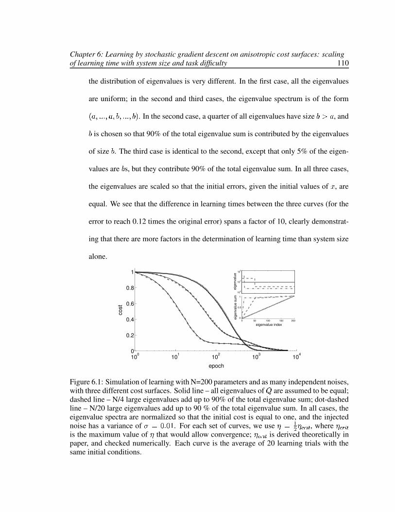
Chapter 6: Learning by stochastic gradient descent on anisotropic cost surfaces: scalingof learning time with system size and task difficulty 110
the distribution of eigenvalues is very different. In the first case, all the eigenvalues
are uniform; in the second and third cases, the eigenvalue spectrum is of the formO % n©u�uÖu�n % nv&�n©u�uÖu�nv&�R . In the second case, a quarter of all eigenvalues have size &s� % , and& is chosen so that 90% of the total eigenvalue sum is contributed by the eigenvalues
of size & . The third case is identical to the second, except that only 5% of the eigen-
values are & s, but they contribute 90% of the total eigenvalue sum. In all three cases,
the eigenvalues are scaled so that the initial errors, given the initial values of ± , are
equal. We see that the difference in learning times between the three curves (for the
error to reach 0.12 times the original error) spans a factor of 10, clearly demonstrat-
ing that there are more factors in the determination of learning time than system size
alone.
100
101
102
103
104
0
0.2
0.4
0.6
0.8
1
eigenvalue index
eige
nval
ueei
genv
alue
sum
0 50 100 150 2000
0.5
1
104
102
100
epoch
cost
Figure 6.1: Simulation of learning with N=200 parameters and as many independent noises,with three different cost surfaces. Solid line – all eigenvalues of á are assumed to be equal;dashed line – N/4 large eigenvalues add up to 90% of the total eigenvalue sum; dot-dashedline – N/20 large eigenvalues add up to 90 % of the total eigenvalue sum. In all cases, theeigenvalue spectra are normalized so that the initial cost is equal to one, and the injectednoise has a variance of � [ý�ÅuÊ��� . For each set of curves, we use �Ò[ g� �<Ç y � ë , where �<Ç y � ëis the maximum value of � that would allow convergence; �QÇ y � ë is derived theoretically inpaper, and checked numerically. Each curve is the average of 20 learning trials with thesame initial conditions.

Chapter 6: Learning by stochastic gradient descent on anisotropic cost surfaces: scalingof learning time with system size and task difficulty 111
The concept that learning will depend on the shape of the cost function is not itself
new. The dependence of learning speed on the cost surface shape, as determined by
the eigenvalues of the Hessian matrix, has been well studied in the literature on direct
gradient learning rules [52, ?]. However, the effect of anisotropic cost surfaces on the
speed of learning with stochastic gradient descent has not been dealt with. Results on
the scalability of stochastic gradient learning have tended to focus solely on system
size. We expand the discussion to include the eigenvalue spectrum of á , which gives
more detailed information about the specific problem to be learned. We show that
learning on an isotropic surface [59] provides the worst-case picture of learning with
stochastic gradient descent. Intuitively, this is because in the case of learning on an
isotropic surface, all directions in parameter space are equally important, and so the
number of effective dimensions is equal to the actual size of the system, and equal
also to the number of independent noises in the system. If learning depends predomi-
nantly on the decrease of error along a few eigenvectors, the effective dimensionality
of the learning problem is much smaller than the actual system size, and learning can
proceed relatively rapidly.
Despite the intuitive argument made above, the precise way in which the cost func-
tion valley shape affects learning by stochastic gradient is not clear, because of the
different nature of learning by random walk in a multidimensional space than by
direct gradient descent. One could imagine that most learning slow-downs result-
ing from anisotropies in the valley shape would be completely overshadowed by the
slowdowns inherent in learning by random search in a large dimensional space; per-

Chapter 6: Learning by stochastic gradient descent on anisotropic cost surfaces: scalingof learning time with system size and task difficulty 112
haps only anisotropies larger than the system size could visibly affect convergence
if learning is by stochastic gradient. To address these issues, we analytically com-
pute the ensemble-averaged learning curves for stochastic gradient descent on an
anisotropic cost function.
6.1 Learning curve
Since the cost function is quadratic in ± and since there arev
noises injected into
the system, driving independent exploration in as many dimensions, we must track
the learning process by following the evolution of thev
variables ± �� . If we write ±and + in the eigenvector basis of á , then after one iteration the prescribed change in±q� is given by
� ±Î�Õ[ú��×Ø m 2 +Yáz± � ¨ g� +�á + � 5�+�� ; we use this to obtain an expression
for OG± � g �� R � as a function of OZ± � � �� R � , and compute the expectation over the distribution
of + to get:
é3OG± � g �� R"�$ê�h�[ SSOG± � � �� R"�\� � � ã �%OZ± � � �� RP� ¨ �Å� N � ã �� OZ± � � �� RP� ¨ d U ã �U OG± � � �U R"� P Y¨ � � � � � N � ã ���¨ ã � d U ã U ¨ � d U ã �Uè¨ O d U ã U�R � P (6.3)
If we define Ù�� � é=± �� ê , we can express the error as é � � g � êè[ g� Ð � ã �?Ù � g �� . Moreover,
Equation (6.38) is linear in ÙV� ; this allows us to write the evolution of ÙY� as a function
of the number of learning iterations, Q , in the form of a recursion relation: Ù�� ë Ì g �Õ[� Ù � ë � ¨ � u The recursion matrix � is a function of the eigenvalues of the original cost
matrix á , and of the learning rate � ; it is given by �ß��U®[ÙH���UVOP� � � � ã � ¨ � � � ã �� R ¨

Chapter 6: Learning by stochastic gradient descent on anisotropic cost surfaces: scalingof learning time with system size and task difficulty 113� � ã �U , and � �\[ g� � � � � 2 � ã ��2¨ ã ��Ð U ã U ¨ � Ð U ã �U⨠ODÐ U ã U�R � 5 is a residual term.
The central advantage of being able to write down the evolution of Ù in terms of a
recursion relation governed by a recursion matrix, is that the entire learning process
depends on just the eigenvalues of � , and not on the specific intermediate values of± or Ù . Thus, we can write down Ùi� ë �ª[ � ë Ù�� � � ¨ Ð ë ¹ gy e � � y � u If Ú is the column
matrix of the normalized eigenvectors Ú æ of � , and � æ are the associated eigenvalues,
then the learning curve for stochastic gradient descent on the anisotropic cost surface� [ g� ±cáz± � is given by:
� � ë � [ d ��� æ ã ��Ú � æeÛÙ æ � ëæ ¨ ÞSñ©ïrí�ógÜqöV÷ (6.4)
[ d�I� æ � U ã ��Ú � æ � ëæ O-Ú ¹ g R æ U�OZ± � � �U RP� ¨ Þrñ�ïrí�ógÜqöV÷ (6.5)
where ÛÙ æ [ Ð U O-Ú ¹ g R æ U$Ù¥U is the projection of Ù onto Ú æ in the eigenvector basis
of � , and the residual term is Ð ë ¹ gy e � Ð æ � yæ O-Ú ¹ g R æ U��ÕU . Equation (6.5) is therefore
the full learning curve, and the problem of learning with stochastic gradient descent
on anisotropic learning surfaces is solved, if we can compute the eigenvalues and
eigenvectors of � . In fact, it is not possible to derive the eigenvalue spectrum of � for
general á , because of the non-trivial dependence of � on the learning rate parameter� as well as on the eigenvalues of á .
For learning to converge, the eigenvalues ��� of the recursion matrix must lie inÃf�|�Vn¥�©Æ . The learning rate � must be chosen to ensure that this condition is satis-
fied. To do so we need to explicitly compute ���POZ��R .

Chapter 6: Learning by stochastic gradient descent on anisotropic cost surfaces: scalingof learning time with system size and task difficulty 114
6.2 Bounds on the learning rate
While we do not know how to solve for the eigenvalues of � in general, we can derive
expressions for them in special cases that are nevertheless of considerable interest.
Case 1 The simplest case to consider is if thevÝ�¿v
matrix á has ° § vuniform
eigenvalues,ã � [ % 3h� § ° , and the remaining
v ��° eigenvalues are 0. It is easy
to verify that the eigenvalues of � are:
�*Ç«[ �Ì� � � % ¨ O-° ¨ � RP�Å� % � õVî�ñ ô©õ ´T´ õYî ´ õ�ó�ñ (6.6)�97 [ �Ì� � � % ¨ � �Å� % � ´ � � ó�íÞÉ ñ�Þrñ�î�ðrí?öV÷ ´ õÅó�ñ©ï (6.7)� � [ � ´ Ü�÷�ðríIò�÷�íIô©íÖð�ßáà � ´ (6.8)
These eigenvalues are all real and nonnegative, 3 % n3� �×� . For convergence, both�9Ç and �*7 must be in Ãf�x�Yn¥�©Æ ; since we know they are positive, the only non-trivial
bound is from above; thus, we see from the union of constraints for both eigenvalues
that for convergence of the error, we must have � § � § �¦Ç y � ë [ �¥ � ¡ Ì � � . The special
case of ° [ vis the case where all the eigenvalues of á are equal and nonzero,
and corresponds to learning on an isotropic surface, as considered by Werfel et al in
[59]. Under the isotropic eigenvalue assumption, our conditions for convergence and
solution for the learning curve agree with the results of [59].
Case 2 Next consider the case where á has two distinct non-zero eigenvalues, %(of multiplicity ° ), and &É� % (of multiplicity � ); ° ¨ �²[ v
. We solve for the
eigenvalues of � to get (see Appendix):

Chapter 6: Learning by stochastic gradient descent on anisotropic cost surfaces: scalingof learning time with system size and task difficulty 115
�97 ¡ [ �â� � � % ¨ � �Å� % � ÚU7 ¡ [ âãä � ¡�åWæç (m-1 differential modes)
�97 � [ �Ì� � �*& ¨ � �Å�n&.� ÚU7 � [ âãä �� �åWæç (n-1 differential modes)
�*è ÚZèÉ[ g� ¡ Ì ��é m êcë<ì � âãä � ¡H � è � � �å æç (2 modes)
The eigenvalues �>è are obtained from equating two equivalent expressions for the
numbers H � è � , H � è � [ × m¥m ¡í ë ¹ � g ¹ � × ¤ Ì × m ¤ m ��� Ì � �Þ� [ í ë ¹ � g ¹ � ×
¥ Ì × m¥m � ¡ Ì � �Þ�× m ¤ m � . The °°��� ° -
dimensional vectors labeled by � ¡ are normalized orthogonal differential modes,
named because Ð � O�� ¡ RP� [ý� for each of the modes; Ú<7 ¡ arev
-dimensional zero-
padded versions of the vectors � ¡ . The same is true for the �¦� � differential modes� � , and the corresponding vectors Ú<7 � .We must once again solve for convergence criteria in terms of the allowed learning
rates � , by imposing that �¾E à �x�Yn¥�©Æ . The differential mode eigenvalues are clearly
real and positive, and provide necessary bounds on � : �g7 ¡ Ñ � [ î � § � §g¥ ]r�97 � Ñ �o[ î � § � § g¤ . Since & � % , the combined constraint from the two sets
of differential modes becomes � § � § g¤ . The remaining constraints come from the
two remaining modes. With a little work, is possible to show that the eigenvalues �"èare also real and positive (see Appendix), and that they provide constraints on � so
that either � § �Å͹ , or �ï� �ÅÍÌ , where

Chapter 6: Learning by stochastic gradient descent on anisotropic cost surfaces: scalingof learning time with system size and task difficulty 116
� Íè [ 2 % O,° ¨ � R ¨ & O-� ¨ � R 5 �ñð 2 % O,° ¨ � R ¨ & O,� ¨ � R 5 � ��� % & O-� ¨ ° ¨ � R� % & O-� ¨ ° ¨ � R (6.9)
One can show, from Equation (6.9), that ��Íè is real, and that ��Íè � � . The allowed
range for � lies in the intersection of all the bounds, and will depend on where g¤ lies
relative to � Íè . We can expand the expression for � Íè to first order in �Fò¬ ��� Ì ¡ Ì � ��»� ¡ Ì � � Ì ò¬ ��� Ì � �Þ� mto see that
� ͹ � �% O,° ¨ � R ¨ & O-� ¨ � R Ñ �& n (6.10)
� ÍÌ � % O,° ¨ � R ¨ & O-� ¨ � R% & O-� ¨ ° ¨ � R � �& (6.11)
where the latter inequality for ��ÍÌ holds because &s� % .Thus, the intersection of constraints is that � Ñ �QÇ y � ë , where
�<Ç y � ë [�� ͹ � �% O,° ¨ � R ¨ & O-� ¨ � R (6.12)
6.3 Learning time and scaling
The iteration matrix � is a function of both � and the eigenvalues of á . Since we
now have values of �FÇ y � ë for both the isotropic and anisotropic cases, we can use the
them to compute the eigenvalues of � , and derive the dependence of learning time on% nn& nv�ùn and ° .

Chapter 6: Learning by stochastic gradient descent on anisotropic cost surfaces: scalingof learning time with system size and task difficulty 117
Case 1 (Isotropic learning) For ease of comparison with Case 2 below, we assume
that á has � ¨ ° non-zero eigenvalues of size % . We put �½[ó×�ô p � s� [ g¥ � ¡ Ì � Ì � � , and
find that
� ÍÇ [ ��� �O,� ¨ ° ¨ � R (6.13)� Í7 [ ��� �O,� ¨ ° ¨ � R ¨ �O-� ¨ ° ¨ � R � (6.14)
For each mode, the learning time can be defined to be the number of iterations re-
quried for the error along that mode to decrease to some fraction of the initial error.
If this fraction is defined to be Î , and if � ͺ �Ø��� � ±µn then
¢ º OlÎ.R\[ ÷Iõ<zÎOlÎ.R÷IõFzÎOP�Ì� � ±hR � ÷IõFzÎO gÍ R� ± (6.15)
where ¢ º OlÎ.R is the number of iterations needed for mode ± to reach Î times the initial
error along that direction. The larger the value of ± , the faster that mode will learn.
We see that
¢�Ç�O-Î.Rì� � O-� ¨ ° ¨ � R�÷IõFzÎO � Î R (6.16)¢�7�O-Î.Rì� O,� ¨ ° ¨ � R�÷�õFzqO � Î R (6.17)
Case 2 (Anisotropic learning) Recall that á is assumed to have ° eigenvalues of
size % , and � eigenvalues of size & . Using the allowed bounds for � , we put � [×�ô p � s� [ g¥ � ¡ Ì � � Ì ¤ ��� Ì � � ; now we may solve for the resulting eigenvalues ��� of � . The
expressions for �*7 ¡ nr�97 � give

Chapter 6: Learning by stochastic gradient descent on anisotropic cost surfaces: scalingof learning time with system size and task difficulty 118
� Í7 ¡ [ �Ì� � %O-° ¨ � R % ¨ O,� ¨ � R6& ¨ � % �OrO-° ¨ � R % ¨ O-� ¨ � RX&�R � (6.18)
� Í7 � [ �Ì� � &O-° ¨ � R % ¨ O,� ¨ � R6& ¨ � & �OrO-° ¨ � R % ¨ O-� ¨ � RX&�R � (6.19)
Since &�· % ��� and g� ¡ Ì � � Ì ��� Ì � ��� ¤ » ¥ � Ñ g� , it is clear that �hÍ7 � Ñ �hÍ7 ¡ . The expressions
for � Íè , which are obtained by substituting �Ô[o�QÇ y � ë · � into Equation (6.31), are more
complicated:
� Íè [ N �Ì� % ¨ &L ¨ õL � P � &Õ� %L N � ¨ ²õ� LßO-&è� % R P � ¨ °ï� % � & �Ol&è� % R � L � (6.20)
where L � O % O-° ¨ � R ¨ & O,� ¨ � RrR�n õ � O % � O-° ¨ � R ¨ & � O,� ¨ � RrR$n and ²õ �O % � O-° ¨ � R2�ö& � O-� ¨ � RrR . However, to leading order (a reasonable approximation,
especially for � Ì , as confirmed by numerics: see Figure 6.2), we find that
� ÍÌ � �Ì� � %O-° ¨ � R % ¨ O-� ¨ � R6& (6.21)� ͹ � �Ì� � &O-° ¨ � R % ¨ O-� ¨ � R6& (6.22)
and comparing these to the expressions of Equations (6.18), we see that � ͹ �^� Í7 � Ñ�hÍ7 ¡ � �hÍÌ . In other words, the � � � differential modes O=��n.� � R and the modeOP� ¡ nnH � ¹ � � � R are learned roughly equally fast, and faster than the °ú��� differential
modes O�� ¡ n.�YR and O"� ¡ nnH � Ì � � � R .Applying Equation (6.15), we find that

Chapter 6: Learning by stochastic gradient descent on anisotropic cost surfaces: scalingof learning time with system size and task difficulty 119
0.6
0.8
1
101
102
103 10
40.6
0.8
1
N
a=1, b=100
a=1, b=5
gdn
gdm
gdm
g+
gdn
g+,g-
g-
Figure 6.2: Plotted are the four distinct eigenvalues of the recursion matrix � . Top Theeigenvalues of the cost matrix á are % [ � and &�[ � . Bottom The eigenvalues of á are% [�� and &Ì[�� �Y� . In both plots, the system size,
v, is varied between 10 and 4000;
v ·�of the eigenvalues are & , while the remaining are % ; finally, �Ô[��¦Ç y � ë · � . It is clear from thefigure that � Í7 ¡ ���hÍÌ n and that � Í7 � and �h͹ bunch together.
¢�7 ¡ OlÎ.R$n�¢ Ì OlÎ.Rì� 2 O-° ¨ � R ¨ O-� ¨ � R &% 5µ÷IõFzÎO � Î R (6.23)¢�7 � OlÎ.R$n�¢ ¹ OlÎ.Rì� O-° ¨ � R ¨ O-� ¨ � R ¤¥
Ol&�· % R ÷IõFzÎO � Î R (6.24)
We can further simplify the expression of Equation (6.5) for the learning curve. Since
the components of a differential mode sum to zero, Ð � ã ��Ú � æ [�� if Ú æ is a differential
mode andã �à[ % 3h�Sn which is the case in the isotropic case. For the differential
modes ä in the anisotropic case also, Ð � ã ��Ú�� æ [°� . Hence, the only contribution
to the cost, and to the learning process, comes from the remaining, non-differential
modes. � � ë �÷Rø } [ OZ� ÍÇ R ë � � (6.25)� � ë �´Âù ÷Rø } [ OZ� ÍÌ R ë � Ì ¨ OG� ͹ R ë � ¹ (6.26)
where the initial cost in the isotropic learning problem is� � � % Ð U OZ± � � �U R � , and in

Chapter 6: Learning by stochastic gradient descent on anisotropic cost surfaces: scalingof learning time with system size and task difficulty 120
the anisotropic learning problem is� � [ � Ì ¨ � ¹ , with
� Ì � ¡ ¥ Ì é-úF� ¤¡ Ì é mú � Ð U O,Ú ¹ g R ` ¹ g%� U�OG± � � �U R � nand
� ¹ � ¡ ¥ Ì éÂûF� ¤¡ Ì é mû � Ð U O,Ú ¹ g R ` � U OZ± � � �U R � . The expression for Ú ¹ g is given in the ap-
pendix.
The final learning curve for stochastic gradient descent on an isotropic cost surface,
in Equation (6.25), is a single exponential, as in the case of direct gradient descent
(see below), but with a different learning speed. The final learning curve, Equation
(6.26), for learning on a cost surface with eigenvalue spectrum O % n©u�uÖu�n % nv&�n©u�uÖu�nv&�R , is
bi-exponential, with two time-constants of decay, once again in agreement with the
direct gradient case, but with different learning speeds. There is an important differ-
ence, however, which we will discuss below.
6.3.1 Comparison of anisotropic and isotropic stochastic learning
As we saw in Figure 6.1, if a subset of the eigenvalues of á provide the bulk of
the error, then learning can be much faster than if all the eigenvalues are equally
involved. That is, it is possible, if we are not concerned about error very close to zero,
for learning with anisotropic cost surfaces to be much faster than with an isotropic
cost surface. With the help of the analysis of the past few sections, and results of the
analysis presented in the last section, we can quantify this statement.
From Equations (6.25)–(6.26), we see that if � ¹ ç �*ÇÔç � Ì then the total error
in the anisotropic case will decrease much more rapidly than the total error in the
isotropic case, until� � ë � [ � Ì ·�O � Ì ¨ � ¹ R , when learning on the isotropic cost
surface will overtake anisotropic learning. If� ¹ forms a major part of the total error

Chapter 6: Learning by stochastic gradient descent on anisotropic cost surfaces: scalingof learning time with system size and task difficulty 121
in the anisotropic case, i.e., if� ¹ # � Ì , then the overall learning will appear faster
in the anisotropic case than in the isotropic case. Below, we consider the actual
relative sizes of � ÍÌ nr�h͹ , and �*Ç .Assuming that � ¨ ° [ v
is large, we write down the approximate convergence
times with isotropic and anisotropic learning. In the isotropic case, all modes are
equally important and learning time scales like ¢ü� O,� ¨ ° ¨ � Rf� v. In the
anisotropic case, let us consider the following case: the � modes with eigenvalue &contribute to a fraction ] of the summed total of the eigenvalues of á . Then,
¢ ÷Rø } � v(6.27)¢ ´Âù ÷Rø }¤ ��� ¨ �ÚOP�Ì��] R] (6.28)¢ ´Âù ÷Rø }¥ � v ¨ v ]¦�?�O"�Ì��] R (6.29)
If ] is close to one, and �lç v, then OG¢ ´Âù ÷Rø }¤ �ý� Rsç OZ¢ ÷Rø } � v Rsç ¢ ´Âù ÷Rø }¥
; thus,
learning along the fast modes of the anisotropic surface would be much faster than
learning along the isotropic surface; if � is independent ofv
, that is, if the number
of important modes does not scale withv
, then learning could be rather fast, and not
scale asv
, but as � .
Let us compare these predictions with the example of Figure 6.1: in one case,v · � �
of the eigenvalues were assumed to comprise 90% of the total eigenvalue sum, with& [ �±¨Å� % . With these numbers, ¢ ÷Rø } � v nr¢ ´Âù ÷Rø }¤ � v · � � , while ¢ ´Âù ÷Rø }¥ �ÿþ v u Thus
we expect that for the anisotropic cost surface (dot-dashed grey curve), learning along
the � fast modes will more rapid, by a factor of 20, than learning along an isotropic
surface (solid grey curve); the anisotropic learning curve should moreover display a

Chapter 6: Learning by stochastic gradient descent on anisotropic cost surfaces: scalingof learning time with system size and task difficulty 122
‘knee’, marking the transition from learning along the fast modes to learning along
the slower modes. Finally, the full learning curve in the anisotropic case should be
faster than the isotropic learning curve until an error is reached where learning is
dominated by the slow mode; at this point, learning will be faster, by a factor of 9,
for the isotropic surface. Comparing the dot-dashed and solid grey curves, we see
that the difference in learning time to reach down to an error of 10 % of the initial
error, which marks the begining of the knee, is a factor of 10–20, in agreement with
our expectations. The knee leads to a phase of learning of the slow mode; when
plotted on a log-linear scale, the two anisotropic learning curves look linear with a
transition between two separate slopes, while the isotropic learning curve is linear.
6.3.2 Comparison with direct gradient learning
The analysis for direct gradient descent on this class of quadratic cost functions for
linear networks is much simpler. The recursion matrix for Ù in this case is � [H$�(UVOP�Ú� � ã �?R � ; this matrix is purely diagonal, and unlike the stochastic case where the
different learning modes are entangled, here learning along each mode can progress
independently. There is no residual error. The eigenvaluesÛ ����Ü of � are triviallyÛ OP�x�o� ã �?R � Ü , and the convergence condition � �Å� � Ñ ��3à� gives � Ñ � · ã � for each
mode. The intersection of all the bounds is
� Ñ �<Ç y � ë [ �ãmax
(6.30)
whereã ³µ´D¶ is the largest eigenvalue in the spectrum of á . The optimal � for fastest
convergence is ��Íx[ g� �<Ç y � ë [ g�max
. For modes withã Ñ ã
max, the number of steps

Chapter 6: Learning by stochastic gradient descent on anisotropic cost surfaces: scalingof learning time with system size and task difficulty 123
needed for this mode to go below the fraction Î of the initial error will be
¢ËOlÎ3RÚ[ �� ÷Iõ<z Î÷Iõ<zÎO"�â� ã · ã max R uThese exact results for arbitrary eigenvalue spectra
Û�ã ��Ü can be applied to the two
special cases considered for stochastic learning above. In Case 1 (ã �ß[ % 3à� ), ��ÍÌ[��· % , and so ��� [��B3 � , and the error goes to 0 in one step. In Case 2 ( ° eigenvalues
of size % and � of size &ª� % ), ��Íz[ý��·Z& ; thus, the top � eigenmodes converge to 0
error after one step, and error along the remaining ° modes decreases by OP� � % ·<&�R � ë ,so that
� � ë � likewise goes as OP��� % ·<&�R � ë independent of ° and � . ¢ ¡ OlÎ.RÚ[ g� |R}�~ Í|R}�~ � g ¹¥ » ¤ � ;¢ � O-Î.Rà[û� 3áÎ . The ratio of the learning speed for direct as compared to stochastic
gradient descent scales linearly with ° and � , paralleling the result derived in [59].
Interestingly, in contrast to the stochastic case however, direct gradient learning on
an isotropic cost surface is always faster or as fast as any of the modes in anisotropic
learning. To summarize the difference, we found that with stochastic gradient learn-
ing, some modes on an anisotropic cost surface can be learnt much faster than the
modes in isotropic learning. With direct gradient, however, there are no modes in
the anisotropic case that can learn faster than in the isotropic case; in the most favor-
able scenario, some of the anisotropic modes can be equally fast, but not faster than,
isotropic learning. Thus, in more realistic scenarios where learning is by stochastic
gradient, an anisotropic learning problem need not be automatically slower than an
isotropic one; in fact, the reverse may be true.

Chapter 6: Learning by stochastic gradient descent on anisotropic cost surfaces: scalingof learning time with system size and task difficulty 124
6.4 Applications to neural network learning
The preceeding analysis, of learning with stochastic gradient descent on a general
quadratic cost function, can be applied directly to learning with weight or node per-
turbation in two different linear neural networks.
– Learning by weight perturbation in a single layer network (Figure 6.3).
Assume the network hasv
input units, 1 output unit, and is being trained to learnÇ patterns, and define ± � L to be the layer of plastic network weights. Then, the
cost is� [ÈL�á|L � , where áØ[{¯F¯ � is the covariance matrix of the input patterns.
Learning by weight perturbation gives exactly the same update rule for L as learning
by stochastic gradient descent, as described in the past sections.
– Learning in a network with one hidden layer and a single plastic layer of weights
(Figure 6.3).
We assume the network hasv � input units,
vËwhidden units,
vË{output units, and is
being trained to learn 1 pattern, with weight or node perturbation. The weights Lfrom the input to the hidden layer are assumed to be plastic, and the weights M from
the hidden layer to the outputs are assumed fixed. In weight perturbation, only the
plastic weights are perturbed, while in node perturbation only the units postsynaptic
to the plastic weights are perturbed. Then, the cost is� [ OP� � L � áËL ��R , whereá [ØM � M . Learning with either rule, on one pattern, follows learning as described
in the past sections. The results could also apply to the learning of Ç Ñ vpatterns

Chapter 6: Learning by stochastic gradient descent on anisotropic cost surfaces: scalingof learning time with system size and task difficulty 125
if the Ç patterns are orthogonal, such that ¯<¯ � [�Ä . For more details, cf. the section
on scaling in Chapter ch:birdsong.
W
z
(a) 1-layer network, weight
perturbation
W
A
(b) 2-layer network, node
perturbation
Figure 6.3: The analysis of stochastic gradient descent on an anisotropic quadratic costfunction can be applied directly to problems in neural network learning. The solutions canbe mapped directly to the learning, with weight perturbation, of P patterns in a single-layerlinear perceptron, where ± � L is the set weights from
vinputs to a single output, andá [�¯<¯ � is the
v{� vcovariance matrix of the Ç inputs. Alternatively, the analysis applies
to the learning of one pattern in a 2-layer network with one hidden layer and multiple outputunits.
Next, we compute the eigenvalue spectrum of the cost function of a real-world hand-
written digit data set, used to train neural networks to perform digit recognition,
Figure (??).
We see from the cumulative sum of the eigenvalues that the bulk ( � 80 %) of the
eigenvalue sum comes from the top 40 eigenvalues. In other words, it is only a few
eigenvectors (40 out of 784 possible modes), corresponding to the top few eigen-
values, that really need to be learned. Thus, learning time should depend not on��· v [���·F¨V�� , but rather as ��·��� , or the number of vectors with large eigenvalue, the
principal components.

Chapter 6: Learning by stochastic gradient descent on anisotropic cost surfaces: scalingof learning time with system size and task difficulty 126
0 100 200 300 400 500 600 700
10−200
10−150
10−100
10−50
100
0 10 20 30
108
0 200 400 6001
1.5
2
2.5
3x 10⁹
0 50 1001
1.5
2
2.5
x 109
Eigenvalue #
Figure 6.4: Eigenvalue spectrum and derived quantities for a data set of 550 exemplars ofthe digit ‘7’ from the NIST handwritten digit database []. Main figure, eigenvalue spectrumof the covariance matrix of these inputs, á [ ¯F¯ � . Insets: top left, closeup of largesteigenvalues; bottom left, cumulative sum of eigenvalues; bottom right, closeup of first 100terms of the cumulative sum. The first 30-40 eigenvectors make up the bulk of the variationin the data set, by principal components analysis.
We can compute the eigenvalues of the combined covariance matrix of 5000 samples
of all 10 digits, from 0 to 9, and find once again that the top 40 eigenvalues contribute
¿80% of the total eigenvalue sum. Examining by eye the reconstruction of the digits
based on the first Ç principal components, we found that Ç��¬Y� is sufficient to
identify almost all digits; in other words, 40 eigenvectors make up the bulk of the
variation in the data set.
Studies of scaling behavior with network size frequently rely on the unwritten as-
sumption that the difficulty of the task the network is trained on grows along with
the size of the network. While this is sometimes true, it is not so in many real-world
cases. Figure 6.5 shows the cumulative sums of the eigenvalue spectra for the dataset

Chapter 6: Learning by stochastic gradient descent on anisotropic cost surfaces: scalingof learning time with system size and task difficulty 127
of Figure 6.4, and a variant thereof obtained by reducing the image to half its original
resolution in both linear dimensions. The total number of pixels, and thus number of
eigenvalues, thus decreases by a factor of four; however the number of eigenvalues at
which the cumulative eigenvalue sum levels off—that is, the number of eigenvalues
contributing to the bulk of the variance, and hence the effective dimensionality of the
problem—is nearly unchanged.
0 100 200 300 400 500 600 700108
109
Eigenvalue #
Figure 6.5: Demonstration of the extent of important information in the digit data set. Solidline: cumulative sum of the eigenvalues of the covariance matrix for the digit 7, as in Figure6.4. Dotted line: cumulative sum of all the eigenvalues for a data set generated from thefirst by downsampling the pixel resolution by a factor of two in both linear dimensionsof the image. The latter has only 1/4 as many eigenvalues as the former, but number ofeigenvectors making up the bulk of the eigenvalue sum is about the same in both cases.The first 30 eigenvectors This is an
Note that these results imply that if the difficulty of the task (i.e., the number of
important eigenvectors, or effective dimension of the problem) is kept the same, then
learning time does not increase even as the network size is increased.

Chapter 6: Learning by stochastic gradient descent on anisotropic cost surfaces: scalingof learning time with system size and task difficulty 128
6.5 Appendix
6.5.1 Derivation of �� and bounds on �� is a block matrix,
�¿[ âãä O"�Ì� � % ¨ � % � R�Ä ¨ % � �Y� � & � �Y� �% � �Y� � OP��� � & ¨ � & � R�Ä ¨ & � �V� �å æç
Since any matrix of form ä/Ä ¨ � �V� � has one common mode vector, � , andv �^�
differential modes � (defined as Ð � �Y�Ú[ � ), we guess a similar form for the eigen-
vectors of � : °Ø� � differential modes O=��n.� ¡ R , where Ð � � ¡ � [� , �ª�l� differential
modes O�� � n.��R$n where Ð � � � �è[ý��n and two common modes, OP� ¡ nnH � è � � � R . The dif-
ferential mode eigenvalues, � ¡ and � � are very easy to compute. Here we compute
the two common mode eigenvalues, �gè , and obtain bounds on � from the condition� § ) ¸ OZ�*è R § � .Get a quadratic equation for �>è from solving the eigenvalue equation,
�*è�[ �� � O=M ¨�� R � Ö OZM²� � R � ¨ Y� ���(6.31)
where M � O"�Ú� � � % ¨ O-° ¨ � R"� � % � R$n � � O"�Ú� � �>& ¨ O,� ¨ � R"� � & � R$n.��[$� � � & � n and� [$°¦� � % � . Then,
�c�è� ��O=M ¨�� R ¨ M � �l� � [� (6.32)
where M � OP�µ� � % ¨ O-° ¨ � R % � R$n � � O"�µ� � & ¨ O-� ¨ � RX& � R�n3��[$� & � n and� [$° % � .

Chapter 6: Learning by stochastic gradient descent on anisotropic cost surfaces: scalingof learning time with system size and task difficulty 129
From this we have that
�*è [ �� � OZM ¨�� R � Ö O=M ¨�� R � �lÎO=M � ��� � R � (6.33)[ �� � OZM ¨�� R � Ö O=Mo� � R � ¨ �� � �(6.34)
Notice from their definitions that MËn3� n � and � are positive. From Equation (6.34)
we see therefore that the argument of the square root is positive, so �"è must be real.
Moreover, � Ì nS� ¹ are both positive, with � Ì Ñ � ¹ . The only non-trivial bound on �gèis therefore � Ì Ñ � , which gives
O=M � ��� � R��²OZM ¨�� R ¨ �x� ��u (6.35)
Since MËn.�an � and � each contain � � , this inequality appears to be quartic in � ; when
fully expanded, however, the two lowest powers of � drop out, and we get that
�Å� O % & O-° ¨ � ¨ � RSR��l� O % O-° ¨ � R ¨ &�O,� ¨ � RSR ¨ � � � (6.36)
This is an upward-facing parabola in � , giving allowed values of � to be � Ñ �Î͹ n3�½��ÅÍÌ , where
� Íè [ 2 % O,° ¨ � R ¨ & O-� ¨ � R 5 � ð 2 % O,° ¨ � R ¨ & O,� ¨ � R 5 � ��� % & O-° ¨ � ¨ � R� % & O-° ¨ � ¨ � R (6.37)
6.5.2 Inverse of the � eigenvector matrix
If the cost surface is anisotropic, so that á has an eigenvalue spectrum consisting of° % s and � [ v � ° & s, the eigenvector matrix Ú of � is as described in Section

Chapter 6: Learning by stochastic gradient descent on anisotropic cost surfaces: scalingof learning time with system size and task difficulty 130
??; since the differential modes are orthogonal to each other as well as to the two
remaining modes, the inverse matrix is almost the transpose of Ú . However, the two
non-differential modes couple, and the inverse matrix is
Ú ¹ g [ N Ú�g�n©u�uÖu�nOÚ ` ¹ � n Ú Ì �²O,Ú Ì� Ú ¹ R6Ú ¹��� O-Ú Ì� Ú ¹ R � n Ú ¹ �²O-Ú Ì� Ú ¹ R�Ú Ì�Ì�oO-Ú Ì� Ú ¹ R � P � u6.5.3 Generalization to � �� output units
We proceed in analogy to the 1-output case; now, ± is a matrix of size � �Òv, and� [ ÝßÞ OZ±cáà± � R�u Since there are
v � noises injected into the system, driving in-
dependent exploration in as many dimensions, we need to track allv � variables,±q�A} � , to follow the learning curve. If we write the columns of ± and + in the eigen-
vector basis of á , then after one iteration the prescribed change in ±h�(U is given by� ±q�(Uz[ � ×Ø m¥ 2 ÝßÞ O,+Yáz± � R ¨ g� ÝùÞ¥O,+Yáá+ � RX5�+©�Ê} ; we use this to obtain an expression forOG± � g ��(U R � as a function of OG± � � ��(U R � , and compute the expectation over the distribution of+ to get:
é3OZ± � g ���U R"��ê6h¬[ SSOZ± � � ��(U RP�è� � � ã U�OZ± � � ��(U RP� ¨ �Å� N � ã �U OZ± � � ��(U RP� ¨ d ¥ ¤ ã �¤ OG± � � �¥ ¤ R"� P Y¨ � ��� � � N � ã �Uè¨ �� ã U d X ã X ¨ � � d X ã �X2¨ ��� O d X ã X©R"� P
At this point, however, we notice that it is not possible to write down a linear recur-
sion relation for ± ��(U , because of the presence of the Ð ¥ ¤ ã �¤ ± ���U term in the equation
above. Thus, although it is possible to compute the noise-averaged 1-iteration learn-
ing update, it is not possible to derive a general recursion relation, since the next step

Chapter 6: Learning by stochastic gradient descent on anisotropic cost surfaces: scalingof learning time with system size and task difficulty 131
in the recursion depends in detail on the values of ± in the preceding step. This is
an obstacle that prevents further analysis of the multiple-output stochastic gradient
learning problem.

Bibliography
[1] D. O. Hebb, Organization of Behavior: A Neuropsychological Theory (Wiley,
Inc., ADDRESS, 1949).
[2] T. Bliss and T. Lomo, J Physiol. 232, 331 (1973).
[3] G. Tong, R. Malenka, and R. Nicoll, Neuron 16, 1147 (1996).
[4] H. Markram, J. Lbke, M. Frotscher, and B. Sakmann, Science 275, 213 (1997).
[5] L. Zhang et al., Nature 395, 37 (1998).
[6] G. Bi and M. Poo, J Neurosci 18, 10464 (1998).
[7] D. Amit, N. Brunel, and M. Tsodyks, J Neurosci. 14, 6435 (1994).
[8] S. Dehaene, J. Changeux, and J. Nadal, Proc Natl Acad Sci U S A. 84, 2727
(1987).
[9] T. Nowotny, M. Rabinovich, and H. Abarbanel, Phys Rev E Stat Nonlin Soft
Matter Phys. 68, 011908. Epub 2003 Jul 18. (2003).
[10] S. Loo and M. Bitterman, J Comp Psychol. 106, 29 (1992).
[11] M. Giurfa et al., Nature. 410, 930 (2001).
[12] M. Hammer, Nature 366, 59 (1993).
132

Bibliography 133
[13] M. Hammer, Trends Neurosci. 20, 245 (1997).
[14] M. Hammer and R. Menzel, Learn Mem. 5, 146 (1998).
[15] M. Schwaerzel et al., J Neurosci. 23, 10495 (2003).
[16] J. Mirenowicz and W. Schultz, Nature. 379, 449 (1996).
[17] W. Schultz, Neuron. 36, 241 (2002).
[18] M. Ungless, P. Magill, and J. Bolam, Science. 303, 2040 (2004).
[19] R. Wise, Neuron. 36, 229 (2002).
[20] L. Stein and J. Belluzzi, Neurosci Biobehav Rev. 13, 69 (1989).
[21] H. Stark and H. Scheich, J Neurochem. 68, 691 (1997).
[22] S. Bao, V. Chan, and M. Merzenich, Nature. 412, 79 (2001).
[23] S. Bao, V. Chan, L. Zhang, and M. Merzenich, Proc Natl Acad Sci U S A. 100,
1405 (2003).
[24] M. Kilgard and M. Merzenich, Science. 279, 1714 (1998).
[25] N. Daw, S. Kakade, and P. Dayan, Neural Netw. 15, 603 (2002).
[26] E. Thorndike, Animal Intelligence (Macmillan, New York, ADDRESS, 1911),
p. 244.
[27] C. Gallistel, T. Mark, A. King, and P. Latham, J Exp Psychol Anim Behav
Process. 27, 354 (2001).
[28] M. Jabri and B. Flower, IEEE Transactions on Neural Networks 3, 154 (1992).
[29] B. Widrow and M. Lehr, Proceedings of the IEEE 78, 1415 (1990).
[30] R. Hahnloser, A. Kozhevnikov, and M. Fee, Nature 419, 65 (2002).

Bibliography 134
[31] H. Seung, Neuron. 40, 1063 (2003).
[32] J. Hertz, A. Krogh, and R. Palmer, Introduction to the Theory of Neural Com-
putation (Addison-Wesley, Redwood City, CA, 1991).
[33] C. Koch, Biophysics of Computation: Information Processing in Single Neu-
rons (Oxford University Press, New York, New York 10016, 1999).
[34] S. Haykin, Neural Networks: A Comprehensive Foundation (Prentice Hall, Up-
per Saddle River, New Jersey 07458, 1999).
[35] R. Horn and C. Johnson, Matrix Analysis (Cambridge University Press, Cam-
bridge, UK, 1999).
[36] H. Simpson and D. Vicario, J Neurosci 10, 1541 (1990).
[37] F. Nottebohm, D. Kelley, and J. Paton, J Comp Neurol 207, 344 (1982).
[38] F. Nottebohm, T. Stokes, and C. Leonard, J Comp Neurol 165, 457 (1976).
[39] R. Mooney, J Neurosci 12, 2464 (1992).
[40] L. Stark and D. Perkel, J Neurosci 19, 9107 (1999).
[41] D. Willshaw, O. Buneman, and H. Longuet-Higgins, Nature 222, 960 (1969).
[42] M. Tsodyks and M. Feigelman, Europhys Lett 6, 101 (1988).
[43] C. Meunier, H. Yanai, and S. Amari, Network: Comput. Neural Syst. 2, 469
(1991).
[44] M. Hermann, J. Hertz, and A. Prugel-Bennett, Network 6, 403 (1995).
[45] M. Konishi, Z Tierpsychol 22, 770 (1965).
[46] M. Brainard and A. Doupe, Nat Rev Neurosci. 1, 31 (2000).

Bibliography 135
[47] K. Doya and T. Sejnowski, in Advances in Neural Information Processing Sys-
tems 7, edited by G. Tesauro, D. Touretzky, and T. Leen (MIT Press, Cam-
bridge, MA, 1995), pp. 101–108.
[48] T. Troyer and A. Doupe, J Neurophysiol 84, 1204 (2000).
[49] R. Williams, Machine Learning 8, 229 (1992).
[50] P. Bartlett and J. Baxter, Technical report (unpublished).
[51] A. Yu and D. Margoliash, Science 273, 1871 (1986).
[52] Y. Le Cun, I. Kanter, and S. Solla, Physical Review Letters 66, 2396 (1991).
[53] D. Margoliash, J Neurosci. 6, 1643 (1986).
[54] D. Margoliash and E. Fortune, J Neurosci. 12, 4309 (1992).
[55] S. Volman, J Neurosci. 13, 4737 (1993).
[56] M. Lewicki and M. Konishi, Proc Natl Acad Sci U S A. 92, 5582 (1995).
[57] P. Foldiak, in The Handbook of Brain Theory and Neural Networks, edited by
M. Arbib (MIT Press, Cambridge, MA, 1995), pp. 895–98.
[58] S. Edwards and R. Jones, J Physics A 9, 1595 (1976).
[59] J. Werfel, X. Xie, and H. Seung, in NIPS (PUBLISHER, ADDRESS, 2003).
[60] A. Barto and P. Anandan, IEEE Transactions on Systems, Man, and Cybernetics
15, 360 (1985).
[61] A. Barto, R. Sutton, and C. Anderson, IEEE Transactions on Systems, Man,
and Cybernetics 13, 835 (1983).
[62] W. Thorpe, Bird-Song (Cambridge Univ. Press, Cambridge, 1961).

Bibliography 136
[63] P. Marler, J. Comp. Physiol. Psychol. 71, 1 (1970).
[64] M. Fee, B. Shraiman, B. Pesaran, and P. Mitra, Nature 395, 67 (1998).
[65] O. Tchernichovski, P. Mitra, T. Lints, and F. Nottebohm, Science 291, 2564
(2001).
[66] S. Bottjer, E. Miesner, and A. Arnold, Science. 224, 901 (1984).
[67] C. Scharff and F. Nottebohm, J Neurosci. 11, 2896 (1991).
[68] N. Hessler and A. Doupe, Nat Neurosci. 2, 209 (1999).
[69] R. Canady, G. Burd, T. Devoogd, and F. Nottebohm, J Neurosci. 8, 3770 (1988).
[70] K. Herrmann and A. Arnold, J Neurosci. 11, 2063 (1991).
[71] H. Sakaguchi and N. Saito, Brain Res Dev Brain Res. 95, 245 (1996).
[72] K. Immelmann, in Bird Vocalizations, edited by R. Hinde (Cambridge Univ.
Press, New York, 1969), pp. 61–74.
[73] P. Marler, in Acoustic Behavior of Animals, edited by R. Busnel (Elsevier, Am-
sterdam, 1964).
[74] A. Lombardino and F. Nottebohm, J Neurosci. 20, 5054 (2000).
[75] G. Cauwenberghs, NIPS (1993).
[76] G. Beckers, R. Suthers, and C. T. C, Proc Natl Acad Sci U S A. 100, 7372
(2003).
[77] S. Nowicki, Nature. 325, 53 (1987-7).